Model-Guided Synthesis of Inductive Lemmas for FOL with Least FixpointsDOI: 10.1145/3563354oopslab22main-p769-pJournal: PACMPLVolume: 6OOPSLA219110CCS: Software and its engineering Formal software verificationCCS: Theory of computation Automated reasoningCCS: Theory of computation Logic and verificationCCS: Computing methodologies Machine learning
Abstract.
Recursively defined linked data structures embedded in a pointer-based heap and their properties are naturally expressed in pure first-order logic with least fixpoint definitions (FO+lfp) with background theories. Such logics, unlike pure first-order logic, do not admit even complete procedures. In this paper, we undertake a novel approach for synthesizing inductive hypotheses to prove validity in this logic. The idea is to utilize several kinds of finite first-order models as counterexamples that capture the non-provability and invalidity of formulas to guide the search for inductive hypotheses. We implement our procedures and evaluate them extensively over theorems involving heap data structures that require inductive proofs and demonstrate the effectiveness of our methodology.
Keywords:
Inductive Hypothesis Synthesis, Learning Logics, Counterexample-Guided Inductive Synthesis, First Order Logic with Least Fixpoints, Verifying Linked Data Structures1. Introduction
One of the key revolutions that has spurred program verification is automated reasoning of logics. Particularly, in deductive verification, engineers write inductive invariants that punctuate recursive loops and contracts for methods and then use logical analysis to reason with verification conditions that correspond to correctness of small, loop-free snippets. In this realm, automatic reasoning in combinations of quantifier-free theories using SMT solvers has been particularly useful; in turn, these tools are based on the logics having a decidable validity (and satisfiability) problem (Bradley and Manna 2007; Barrett et al. 2011).
However, reasoning even with loop-free snippets of programs is challenging when the code manipulates linked data structures embedded in pointer-based heaps. Data structures are finite but unbounded structures that are often characterized using recursive definitions whose semantics are defined using both quantifiers and least fixpoints.
First-order logic with least fixpoint definitions (FO+lfp) which accesses various background sorts or theories (e.g., integers and sets) is a powerful extension of first-order logic (FOL) that can define data structures and express their properties. For example, fairly expressive dialects of separation logic have been translated to FO+lfp in order to aid automated reasoning (Calcagno et al. 2005; Madhusudan et al. 2012; Qiu et al. 2013; Pek et al. 2014; Suter et al. 2010; Löding et al. 2018; Murali et al. 2020). The focus of this paper is automated reasoning for first-order logics with least fixpoint definitions or recursive definitions that utilize SMT solvers for quantifier-free reasoning.
The novel automation of FO+lfp reasoning that we propose is a counterexample-guided synthesis of inductive lemmas utilizing complete procedures for pure first-order (FO) reasoning. Our framework requires the FO reasoning procedure to be able to compute counterexample models. The technique we present can be parameterized over any FO reasoning engine able to provide counterexamples for provability. In this paper, we use a particular technique called natural proofs that are based on systematic quantifier instantiation (Löding et al. 2018) and that is able to provide such counterexamples.
The Anatomy of Proofs for FO+lfp : Proofs by Induction. Unlike FOL, FO+lfp does not admit complete procedures11 1 Quick proof: define a “number line” (discrete linear order) using a constant and a unary function (representing successor) with FO axioms expressing that the successor of no element is and that the successor of no two different elements can be the same; second, encode the reachable configurations of a 2-counter machine (which is Turing powerful) as a relation defined using a least fixpoint, and express non-halting of the machine using this relation. This proof in fact shows that even a single recursive definition leads to validity being not recursively enumerable. (i.e., sound proof systems for FO+lfp cannot admit proofs for every theorem). Indeed, on a number line, true addition and true multiplication over the natural numbers are definable using lfp. Hence by Gödel’s incompleteness theorem (Enderton 2001), even quantifier-free logic with recursive definitions has an undecidable validity (and satisfiability) problem.
Humans usually prove properties involving recursive definitions (or least fixpoints) using induction. We consider logics with recursive definitions, where each recursive definition is of the form . Theorems are expressed using first-order logic over a signature that includes these recursive definitions. An inductive proof of a theorem typically involves sub-proofs, which each identify a fairly strong property (the induction hypothesis) and its proof (the induction step).
In this paper, we use a more general notion of induction proofs based on pre-fixpoints, not requiring a concept of size or measure based on natural numbers upon which to induct. We defer this notion until later and instead encourage the reader to simply think of an inductive hypothesis as an inductive lemma and the induction step of the lemma as the pre-fixpoint (PFP) of the lemma.
The main proposal of this paper is to build automated reasoning for FO+lfp with background theories using a combination of (a) complete procedures for FO reasoning to prove theorems and PFPs of lemmas, and (b) counterexample-guided expression synthesis for synthesizing lemmas (i.e., induction hypotheses) that aid in proving a theorem.
We observe that proofs of the induction step (PFP) of the formula can be seen as reasoning using pure first-order logic reasoning without induction. More precisely, we can think of a proof of a theorem in FO+lfp as split into sub-proofs mediated by an induction principle but otherwise consisting of pure FO reasoning. The induction principle says that proving the PFP (induction step) of any lemma proves the lemma.
We can thus view the structure of an induction proof of a theorem as identifying a finite set of lemmas such that:
- •
For each , there is a purely FO proof of using the earlier lemmas as assumptions, and
- •
There is a purely FO proof of with the lemmas from as assumptions.
Notice that proofs of the above form lack any explicit induction proof and the purely FO proofs work under the assumption that each inductive relation is interpreted as a fixpoint definition (not least fixpoint) of the form rather than . The fact that proving suffices as a proof of is implicit and marks the only appeal to the least fixpoint semantics of recursive definitions to argue that the above constitutes a proof of the theorem.
This view of an inductive proof of an FO+lfp formula as pure FO proofs mediated by induction principles suggests a “synthesis reasoning” methodology: (a) synthesize lemmas that are likely to be true and inductively provable, and (b) prove theorems and lemmas using pure FO reasoning.
We emphasize that proving inductive lemmas followed by pure FO reasoning to prove a theorem is itself not new.
For example, the induction axiom schema in Peano arithmetic is:
for any formula . A proof using this axiom can hence be seen as divining formulas and proving lemmas of form by using purely first-order logic over the non-inductive axioms to prove .
The idea of finding proofs by induction by synthesizing inductive hypotheses and proving them using simpler non-inductive reasoning is also not new. This technique is prevalent, for example, in program verification. In this setting, inductive hypotheses are written as loop invariants or method contracts that capture invariants of program states or effects of calling procedures. Synthesizing such invariants and contracts has been explored using a combination of inductive synthesis and reasoning (see work on the ICE framework (Garg et al. 2014), for example, that explicitly takes this approach, and also the related work section). The novelty of our work lies in realizing this technique for proving theorems in FO+lfp using finite models that witness invalidity and non-provability for counterexample-guided synthesis.
Synthesizing Inductive Lemmas. The primary technical contributions of this paper lie in techniques for synthesizing lemmas that (a) can be proved inductively, with their own statement as the induction hypothesis, and (b) aid the proof of a target theorem. We embrace the paradigm of counterexample-guided synthesis that has met impressive success in automating verification and synthesis (e.g., in finding predicates for abstraction (Ball and Rajamani 2002; Namjoshi and Kurshan 2000) or in program synthesis through the CEGIS paradigm (Alur et al. 2015; Solar-Lezama et al. 2007; Solar Lezama 2008)). The salient feature of our technique is the use of finite first-order models that act as counterexamples to guide the search for lemmas.
Suppose a theorem in FO+lfp is desired to be proved valid. Our technique for automated quantified FO reasoning (without least fixpoints), called natural proofs, uses systematic quantifier instantiation followed by SMT-based validation of the resulting quantifier-free formula (Löding et al. 2018; Pek et al. 2014; Qiu et al. 2013). Let be the method that systematically instantiates terms of depth for quantified variables then checks satisfiability of the resulting quantifier-free formula (the latter is a decidable problem). As a simple consequence of Herbrand’s theorem and compactness, we know that this method is complete in the sense that if is a valid formula in FOL, then there is some for which will prove the validity of .
At any point of the lemma synthesis procedure, we would have synthesized a set of potentially useful lemmas already proved valid and then seek a new lemma to help prove .
We utilize three kinds of counterexample models to guide the search for useful and provable lemmas. In our iterative framework for synthesizing useful and provable lemmas, a prover and a synthesizer interact: the synthesizer proposes lemmas, and the prover provides constraints for synthesizing new lemmas. When the synthesizer proposes a lemma, the lemma can be (a) valid and provable using reasoning using existing lemmas, (b) invalid but easily shown to be so using a small model, or (c) valid or invalid, but in either case not provable using and existing lemmas. Note that (a) and (c) cover all cases, and (b) overlaps with (c).
These correspond to the three kinds of counterexamples, which we now name. models guide the search toward lemmas that help prove the theorem and are obtained from the failure to prove using FO reasoning via . models are small, simple counterexamples to validity of proposed lemmas and are obtained by searching for bounded models using SMT solvers. models show non-provability of lemmas and are obtained from failure to prove the PFP of lemmas using FO reasoning via . By utilizing these three kinds of counterexample models, we narrow and guide the search space for lemma synthesis.
The main contribution of this paper is FOSSIL, a novel algorithmic framework for synthesizing lemmas that uses such counterexamples and proves both lemmas and target theorems using FO reasoning. In each round, the algorithm begins with a target theorem and tries proving it using the lemmas synthesized and proved valid so far. If the proof of fails, this failure precipitates a counterexample which will be used to guide the search towards lemmas that do help prove the theorem . The lemma synthesis phase follows, generating a lemma that satisfies the counterexample and then attempting to prove the validity of its PFP. If the proof of the PFP fails, this failure yields either a counterexample (which is a bounded model) if possible or otherwise a counterexample to show non-provability of the PFP. We continue to seek new lemmas guided by these three kinds of counterexamples until a valid lemma is found, at which point we add the new lemma to our set of valid lemmas. We recurse, trying to prove the target theorem . Off-the-shelf synthesis tools do not scale when employed in our framework; however, our synthesis engine works efficiently via constraint solving with SMT solvers, carefully representing counterexamples as ground formulas and formulating synthesis constraints as ground constraints.
Background Theories and Relative Completeness. The techniques for inductive reasoning that we develop in this paper are more involved than as described above. First, many applications, such as program verification, require handling of domains that are constrained to satisfy certain theories, such as arithmetic and sets (sets allow the expression of collections such as “the set of keys stored in a list” in heap-based verification and “the set of heap locations that constitute a list” in heaplets for frame reasoning). Consequently, our framework maintains a foreground sort modeling the heap with pointers as well as multiple background sorts, with the background sorts constrained by theories and that admit Nelson-Oppen style decision procedures for quantifier-free reasoning. In such settings, the work in (Löding et al. 2018) proved that for formulas that quantify only over the foreground sort (i.e., only involving quantification over locations of the heap), systematic quantifier instantiation is still complete. Moreover, satisfiability of quantifier-free formulas after instantiation are supported by SMT solvers, which can also return the three kinds of counterexamples we seek.
Second, we carefully build lemma search to admit relative completeness. We show that if there is a proof of a theorem involving finitely many independently provable lemmas (in the grammar of lemmas provided by the user), then our procedure is guaranteed to eventually find one. More precisely, there are two infinities to explore—one is the search for lemmas and the other is the instantiation depth chosen for finding proofs. As long as our procedure fairly dovetails between these two infinities, it is guaranteed to find a proof.
Evaluation. We implement and evaluate our procedure for a logic that combines an uninterpreted foreground sort with background sorts, where the background sorts have quantifier-free fragments that are decidable using SMT solvers. Our tool framework can employ generic syntax-guided synthesis (SyGuS) engines as well as a custom synthesis tool we built; both of these can synthesize lemmas using FO countermodels that are encoded using logical constraints.
We perform an extensive evaluation on two suites of benchmarks: one of 50 theorems on data structure verification and another of 673 synthetically generated theorems. Our experiments give evidence that the first-order counterexample-based techniques proposed in this paper are effective in synthesizing inductive lemmas and proving theorems. Apart from evaluating the efficiency of our tool, we evaluate the importance of several design decisions and optimizations in our tool. In particular, we study the efficacy of using various kinds of counterexamples and compare our custom synthesis engine with off-the-shelf state-of-the-art synthesis engines.
Lemma synthesis has been studied for related logics, in particular for logics over algebraic datatypes (ADTs) (Reynolds and Kuncak 2015; Yang et al. 2019) and separation logic (Sighireanu et al. 2019; Ta et al. 2017). Though these logics are very different in expressive power and comparisons across tools are hard, we provide a comparison of our tool against tools for these logics on our benchmark theorems using appropriate encodings whenever feasible.
Contributions. The main contributions of this paper are: (1) a counterexample-guided synthesis framework, FOSSIL, for synthesizing inductive lemmas for proving validity in FO+lfp with relative completeness guarantees, (2) the formulation of three kinds of counterexamples that guide synthesis towards lemmas that are relevant to the theorem, lemmas that hold at least on small models, and are provable using induction, (3) efficient synthesis algorithms using specifications formulated as ground formulas, and (4) an implementation and evaluation of FOSSIL on two benchmark suites of theorems in the domain of heap data structures22 2 Our benchmarks and tool can be found at: https://github.com/muraliadithya/FOSSIL.
2. Preliminaries and Problem Definition
In this section, we define the first-order logic framework we work with (first-order logic with recursive definitions that have lfp semantics) and give the problem definition for solving theorems in FO+lfp using synthesis of inductive lemmas and first-order proofs.
2.1. First-Order Logic over Theory-Constrained Background Sorts
The first-order logics (with and without recursive definitions) that we work with are over a multisorted universe that has a single distinguished foreground sort and multiple background sorts. The universes of all these sorts are pairwise disjoint. The foreground sort and the functions and relations that refer to it (as part of the domain or codomain) are entirely uninterpreted (no axioms that constrain them). Background sorts and functions and relations involving only background sorts are constrained by certain theories.
Formally, we work with a signature of the form , where is a finite non-empty set of sorts. is a set of constant symbols, where each has some sort . is a set of function symbols, where each function has a type of the form for some , with . is a set of relation symbols, where each relation has a type of the form .
We assume a designated foreground sort, denoted by . All other sorts in are called background sorts, and for each such background sort we allow the constant symbols of type , function symbols that have type for some , and relation symbols that have type for some to be constrained using an arbitrary theory . All other functions and relations that involve either the foreground sort or multiple background sorts are assumed to be uninterpreted (not constrained by any theory). We consider standard first-order logic (FO) over these multisorted signatures, with standard syntax and semantics, under the combined theories (Enderton 2001).
Counterexamples. We require that validity of quantifier-free logic under the combined theories is decidable. Furthermore, when a quantifier-free formula is not valid, we require this decision procedure to provide models that show satisfiability of the negation of the formula. The truth value of the quantifier-free formula only depends on a finite portion of the model (corresponding to the terms used in the formula, since the formula is quantifier-free). This finite portion can be described by a conjunction of atomic ground formulae. We require models to be given indirectly by such conjunctive ground formulae. Formally, given a quantifier-free formula that is satisfiable, we require that the solver return a conjunctive ground formula such that (a) is satisfiable and (b) is valid. If contains variables, then these are interpreted as or replaced by Skolem constants that are part of the signature of . Intuitively, indicates the existence of one or more models such that is satisfied on all of them. The formula encodes enough information about these models to ensure that is satisfied in them. The following example illustrates these ideas.
Example 2.1 (Counterexample models as conjunctive ground formulas).
Consider the formula where is an uninterpreted function, is of the sort , and is of sort . This formula is invalid, and we can witness the satisfiability of its negation using a model where is interpreted to an element and is interpreted to . can be captured using the formula . Indeed, one can see that is a valid formula. It is also imminent that is satisfiable since realizes it.
In our tools, we work with certain Nelson-Oppen combinable decidable theories (Nelson 1980; de Moura and Bjørner 2008; Bradley and Manna 2007; Nelson and Oppen 1979) (in particular linear arithmetic over integers, sets of integers). These are supported by SMT solvers that guarantee both decidability of quantifier-free formulae as well as model generation as above.
2.2. First-Order Logic with Recursive Definitions (FO+lfp )
Our target theorems are in a dialect of first-order logic over a multisorted universe (universes similar to the one above) but with recursive definitions that have least fixpoint semantics.
We identify a subset of the relational symbols and endow them with definitions; these relations are not directly interpreted by models, rather they are defined uniquely by their definitions. In our work we assume that these recursive definitions only relate elements of the foreground sort. The set of recursive definitions for the symbols are of the form
where , are variables over the foregreound sort, and is a quantifier-free first-order logic formula. Note that a definition can utilize all the sorts and functions/relations in the model. We also assume that there is only one definition for each .
To ensure the well-definedness of definitions, we assume that the symbols in are ordered in layers, and that each that occurs in the definition of is either in a smaller layer, or it is in the same layer and only occurs positively (under an even number of negations) in the definition of (similar to stratified Datalog (Grädel et al. 2007)). The semantics of recursively defined relations is given by the least fixpoint (lfp) that satisfies the relational equations (the condition that each recursive definition only refers positively to recursively defined relations in the same layer ensures that the least fixpoint exists (Tarski 1955))33 3 Our definition of FO+lfp is similar to the one used in Finite Model Theory: see Libkin (Libkin 2004), Chapter 10. Notably, our notion of recursive definitions is more restrictive than general FO+lfp because recursive definitions should only be universally quantified and only over the foreground sort. This technical condition enables us to build effective complete FO validity procedures: see Section 2.4..
Our theoretical treatment assumes that there is only one layer for simplicity. Therefore, each recursive definition only mentions other recursively defined relations positively. However, the results also hold for several layers of recursive definitions, and indeed our experiments utilize them.
Example 2.2 (Linked Lists).
Let be a unary function symbol modeling a pointer of type , i.e., from the foreground sort to the foreground sort. Let nil be a constant of sort , and be a unary relation with the recursive definition
Then, in any model where is interpreted using its lfp definition, holds precisely for those elements that are the head of a finite linked list with as the next pointer. FOL without lfp cannot describe such linked lists (Libkin 2004). Note that unlike Algebraic Datatypes (ADTs), if holds in a model, the lists pointed to by and are not necessarily disjoint and could “merge” in the model. We can also model disjointedness using heaplets, as we show in the following example.
Example 2.3 (Trees and Heaplets).
Consider the following recursive definition for a predicate which expresses that is the root of a binary tree on pointers (left) and (right):
Observe again that since our data structures are unlike ADTS, pointers and may possibly point to the same element (“merge”) in arbitrary heaps/models. Therefore, to define trees we define a recursive definition for the partial function expressing the heaplet of a tree where is a background theory of sets of locations with which we demand that the left and right subtrees are disjoint. This is similar to constraints used in Separation Logic to express trees (Reynolds 2002).
We now state the usual notion of validity/entailment in FO+lfp in the language introduced above.
Definition 2.4 (FO+lfp Entailment).
For a sentence and a set of formulas we write if is true in all models of using the lfp semantics for relations with definitions given in .
We conclude this section with some remarks.
First-Order Abstractions of Recursive Definitions. Given an FO+lfp formula, we can sometimes prove it valid using pure FOL. We can do this by interpreting recursive definitions in to be fixpoint definitions (as opposed to lfp). More precisely, we constrain the relations using FOL as . If is valid under the fixpoint interpretation of recursive relations, then it is of course valid using least fixpoint interpretation as well, but the converse does not hold. Interpreting recursive definitions as fixpoint definitions rather than least fixpoint definitions is hence a form of sound abstraction. We write to denote that is valid using the FO fixpoint abstractions of .
Partial Functions. The reader may have observed in Example 2.3 that we presented a recursively defined function . Although we don’t allow them in the theoretical treatment, our tools support recursively defined partial functions from the foreground sort to both foreground and background sorts (for modeling heaplets of structures, lengths of lists, heights of trees, etc.). However, partial functions can be modeled using two predicates: one recursively defined predicate that captures the domain of the partial function and another predicate defined using only FOL that captures the map of the function.
FO+lfp Fragment. In this work we only handle the validity of formulas whose quantification is purely over the foreground sort. This fragment is well suited for the domain of heap verification that we study. We can model the heap as the foreground sort and express recursively defined functions and properties that only quantify over the heap. However, it is not as powerful as full FO+lfp . For example, the logic cannot talk about array properties (where the array is modeled as a map from indices to values in a domain ) that quantify over integers, which is a background sort. We also cannot express theorems like “For every positive integer , there is a linked list of length ” as this requires universal quantification over the background sort. These restrictions are important as they allow us to leverage practical complete algorithms (Löding et al. 2018) for FOL validity for this restricted fragment in implementing the FOSSIL framework (see Section 2.4).
2.3. The Inductive Lemma Synthesis Problem for Proving FO+lfp Formulas
In this work we develop algorithms that prove an FO+lfp formula valid given a finite set of axioms and a set of recursive definitions with lfp semantics. We want to show that mainly using first-order reasoning. Clearly, if , then as argued above.
We use the following running example to illustrate ideas developed in the sequel:
Example 2.5 (Running Example).
Consider the recursively defined relation defining linked list segments between locations and on the pointer :
Now, consider the following Hoare Triple:
The above triple generates the following Verification Condition (VC) :
We denote by the singleton set containing the definition of . We will use the problem of checking as a running example in this paper. Note that is actually valid in FO+lfp but it is not FO-valid, i.e., holds but does not. This makes the problem a good candidate for lemma synthesis. We describe a run of our algorithm on this example in Section 3.4.
The overall idea in our approach is to use intermediate inductive lemmas to find an FO proof of the goal. We handle a particular fragment of FO+lfp in our work. First, we require the goal to have quantification only over the foreground sort. Second, we only consider lemmas of the form for variables over the foreground sort, a quantifier-free formula , and a recursively defined relation . Finally, we prove lemmas valid using a specific form of induction called the pre-fixpoint (PFP) formula. Given a lemma of the form above, the PFP of expresses that is a pre-fixpoint of the definition of :
where is the formula obtained from by replacing every occurrence of for terms in by . It turns out that if is FO-valid, then is a valid FO+lfp formula, as the following theorem states:
Theorem 2.6.
(Löding et al. 2018) If , then .
We use the above formalism to define the notion of an inductive lemma, as well as the notion of a sequence of lemmas that prove a theorem using FO reasoning.
Definition 2.7 (Inductive Lemmas).
A lemma is inductive for if . If and are clear from the context, we omit them and just say that is inductive.
Example 2.8 (Running Example: Inductive Lemma).
Consider in the setting of Example 2.5 the following lemma :
| () |
which expresses that if we have a list segment pointed to by until , as well as one pointed to by until , then points to a list segment until . It turns out that is inductive i.e., . In other words, the of the lemma is provable in pure FOL, without induction, and with FO abstractions of the definitions (fixpoint instead of least fixpoint).
The crucial part of the proof is the following subformula of :
which is valid given since, according to the definition of , if holds then also holds (in the non-degenerate case).
We now define the notion of proving a theorem using lemmas as well as the synthesis problem that it poses which we tackle in this work.
Definition 2.9 (Sequential Lemmas that Prove a Theorem).
A sequence of lemmas provides an inductive proof of if and for each , is inductive for (i.e., ).
Definition 2.10 (Sequential Lemma Synthesis Problem).
Given a grammar for expressing lemmas and a theorem , find a sequence of lemmas admitted by that provides an inductive proof of (as in Definition 2.9).
Independently Proven Lemmas. We can also define a simpler synthesis problem corresponding to a weaker class of inductive proofs. Specifically, we can require a set of lemmas that are independently proven inductive and help prove a theorem:
Definition 2.11 (Independent Lemmas that Prove a Theorem).
A set of lemmas provides an inductive proof of if and for each , .
The difference between the two classes of proofs is that the inductiveness of lemmas in a sequential proof can depend on previous lemmas. As one might expect, the notion of proof using independent lemmas is strictly weaker than the one that uses a sequence of lemmas. We conclude this section with the running example.
Example 2.12 (Running Example: Lemma Proving a Theorem).
Consider and introduced earlier in the running example. Now, observe that . This is because the crucial part of the validity of is the following formula:
which captures the ‘else’ case of the subformula of (see Example 2.5). We can see that entails the above formula in FO since (informally) is a special case of . Combined with the fact that is inductive (Example 2.8), we have that proves in the sense of Definition 2.9. We illustrate a run of our synthesis algorithm that proves by synthesizing in Section 3.4.
In Section 3 we present our core algorithm FOSSIL for solving the sequential lemma synthesis problem. This algorithm, apart from being sound in producing sequential lemmas that prove the theorem, is accompanied by a relative completeness result: it is guaranteed to find a proof as long as there is a set of independent lemmas that prove the theorem.
2.4. Background: First-Order Validity using Systematic Quantifier Instantiation
In this section we describe the Systematic Quantifier Instantiation (SQI) mechanism for FO validity (without recursive definitions/lfp) that we use, developed in the work (Löding et al. 2018). The results in this section are derived from the work in (Löding et al. 2018) and are not contributions of this paper.
Let be an FO formula. To check the validity of , we negate and Skolemize it — introducing both Skolem constants and Skolem functions — and obtain a purely universally quantified formula such that is valid if and only if is unsatisfiable. Let be of the form where quantifier-free. For a set of ground terms , we denote by the set of all quantifier-free formulas that are obtained by instantiating the variables in by terms in , i.e.,
It follows that if is unsatisfiable then is unsatisfiable and therefore is valid. Since we assume in our setting that satisfiability/validity of quantifier-free formulas is decidable (see Section 2.1), checking whether is unsatisfiable is decidable.
Systematic Quantifier Instantiation. The above suggests a complete semi-decision procedure for validity based on systematic quantifier instantiation (SQI). Let be the formula that we want to check for unsatisfiability where are variables of the foreground sort and is quantifier-free. For any , let denote the set of all ground terms whose type is the foreground sort and are of depth at most (we assume that the signature contains at least one constant symbol for the foreground sort). Then, starting with , we check whether is unsatisfiable. If it is then we halt and report that is valid; otherwise, we increment and repeat. This motivates the following definition:
Definition 2.13 (Provability at depth using SQI).
A formula is provable at depth using SQI if the negated and Skolemized formula is such that is unsatisfiable.∎
The above is a sound procedure, i.e., if is provable at depth using SQI (for some ) then it is clearly valid. It is also a complete procedure for validity in pure first-order logic without any theories (i.e., just uninterpreted functions). This follows from Herbrand’s theorem and the compactness theorem. It turns out that this continues to be a complete procedure in the multisorted setting for the kind of FOL formulas that we work with. i.e., those that quantify only over the foreground sort. We formally state below this result from the work in (Löding et al. 2018):
Theorem 2.14 (From (Löding et al. 2018)).
Let be a formula with quantification only over the foreground sort. Then is valid if and only if there exists such that is provable at depth using SQI.
We implement and use SQI for proving validity of first-order logic formulae in this work.
3. The FOSSIL Algorithm for Sequential Lemma Synthesis
In this section, we present the fundamental contribution of this paper: FOSSIL (First-Order Solver with Synthesis of Inductive Lemmas), our algorithm for solving the Sequential Lemma Synthesis problem formulated in Definition 2.10. Figure 1 shows the components of our framework which we describe in Section 3.1. FOSSIL is a counterexample-based lemma synthesis algorithm that orchestrates interactions between these external components through three kinds of counterexamples. We formally define these counterexamples in Section 3.2. We then present the FOSSIL algorithm in Section 3.3. Finally, we illustrate a run of FOSSIL on our running example in Section 3.4. (the algorithm is guaranteed to find a proof if there is a set of independent lemmas that prove the goal).

3.1. Components of FOSSIL
In this section, we discuss the external components used by the core FOSSIL algorithm. We only describe what these components are, deferring implementation details to Section 6. Let us fix a set of axioms and a set of recursive definitions throughout the following presentation. We also fix a goal formula and a grammar for lemmas. We assume that consists of universally quantified sentences, and that is also a universally quantified sentence (using Skolemization if necessary).
FOSSIL finds a proof of by synthesizing a sequence of lemmas belonging to such that is a sequence of lemmas proving according to Definition 2.9. The high-level external components of FOSSIL are shown as purple boxes/arrows in Figure 1. We describe their abstract interface below in terms of formulae and counterexamples. We encourage the reader to think of counterexamples as finite FO models for now, pending their formalization in Section 3.2. The components of FOSSIL are:
- (1)
First-Order Validity Engine : This is an FO validity checking algorithm based on Systematic Quantifier Instantiation (see Section 2.4). It takes as input a formula and a natural number , and outputs whether valid or unprovable at depth using SQI.
- (2)
Provability Counterexample Generator : This is a counterexample generation module that is part of the FO validity engine. When a formula is found to be unprovable (using term instantiation with terms of depth ) it returns a finite counterexample model. This model is one in which holds. is the negation of the formula instantiated by terms up to depth . Intuitively, the counterexample witnesses the non-provability of using term instantiation with depth terms. Note that finite counterexample models (i.e., where the foreground universe is finite) always exist because is a quantifier-free formula. This module is used to generate the and counterexamples (the inputs being the goal or a proposed lemma respectively). The types of counterexamples are explained below in Section 3.2.
- (3)
Bounded Counterexample Generator : Given an FO+lfp formula and a parameter this module returns a finite model with at most elements in the foreground sort that shows that the formula is not valid, if possible. It may also return that such a model could not be found (because one may not exist at that size). These models interpret recursively defined predicates using the true lfp semantics and will be used as counterexamples.
- (4)
Synthesis Engine : This module synthesizes candidate lemmas. It takes as input a set of counterexample models expressed as quantifier-free constraints and a grammar , and generates an expression in , if one exists, that avoids all counterexamples.
We now turn to the definition of the three kinds of counterexamples used in FOSSIL.
3.2. Counterexamples
FOSSIL is a counterexample-guided algorithm that uses the verification and synthesis components in rounds of lemma proposals. In this section, we define the notion of the various counterexamples that we use.
While counterexamples can be intuitively thought of as finite models for the foreground universe, we will formally treat them as conjunctive ground formulae as described in Section 2.1. For example, consider the model depicting a one-element linked list on the pointer . The foreground universe has two elements, say and , such that and nil is interpreted to be . Then the ground formula with new constant symbols and defines a class of models that contains the intended model. In general, a ground formula captures a class of models where a finite portion of the model is constrained by the formula.
In our algorithm we evaluate formulas over tuples of elements on models represented by a ground formula . We use the notation to indicate that the model contains interpretations for the constants in , and we use this tuple to instantiate the variables of formulas that we evaluate over the model. For example, see lines 8b and 8c of the FOSSIL algorithm (Figure 2). Similarly, we refer to a set of elements interpreted by a model by and use it to evaluate a formula on all tuples over , as in line 8a.
The FOSSIL uses three kinds of counterexamples. Let us fix to be the context formula containing the axioms, recursive definition abstractions, and the valid lemmas discovered so far.
Counterexamples. counterexamples guide the synthesis toward lemmas that help prove the goal. Given a term depth , counterexamples witness non-provability of the goal using term instantiation with depth terms. In other words, this is a counterexample to the non-provability of using the instantiation.
Formally, a counterexample at depth is a satisfiable ground formula such that , where is a tuple of Skolem constants resulting from the Skolemization of the existential quantifiers in the negation of . Such a model witnesses that cannot be proven from by instantiation with terms of depth . We use counterexamples in FOSSIL in lemma synthesis by accessing tuples of elements that correspond to terms in (line 8a in Figure 2). We name these elements and represent them as a set , denoting the counterexample by .
Generating counterexamples: Recall from Section 2.1 that in our setting, for any satisfiable quantifier-free formula , we can obtain a satisfying model as a conjunctive ground formula. When failing to prove using depth term instantiation we obtain a satisfiable conjunctive ground formula from the satisfiability of . This is the counterexample.
Counterexamples. These counterexamples correspond to finite models (i.e., those in which the foreground sort is finite) that falsify a candidate lemma in FO+lfp . Such a model satisfies . When a lemma is proposed, creating a small model in which is false can easily show its invalidity.
Formally, a counterexample for a lemma of the form is represented as a ground formula with constants of the foreground sort such that . The formula can include constraints involving relations in . interprets the recursively defined predicates with lfp semantics. We require that there exists an FO model whose interpretation for predicates in matches their recursive definitions (we describe how we implement this requirement in Section 4.2). Finally, we require .
For example, consider the finite model consisting of two locations, say and , where is the head of a one-element linked list and points to itself on the pointer. This model is captured by the formula . Note that the correct valuation of on this universe is given by the formula.
Generating counterexamples: We fix a bound and use an SMT solver to identify a model with at most elements in the foreground sort that falsifies the lemma, if one exists. We provide further details in Section 4.2 and Section 6.
Counterexamples. counterexamples guide the search towards lemmas that are inductively provable using their PFP. When the PFP of a proposed lemma is found to be unprovable (using depth term instantiation), we obtain a counterexample that witnesses the non-inductiveness of (with respect to the lemmas discovered so far). Note that we do not actually know whether the lemma is valid/invalid or provable/unprovable as it may require discovering other lemmas or a bigger instantiation depth. This is similar to a counterexample, where instead of the target theorem we generate counterexamples to the PFP of a candidate lemma.
Formally, a counterexample for a lemma is a ground formula with such that holds and is satisfiable. The constants are Skolem constants obtained from Skolemizing the existential formula .
Generating counterexamples: Similar to counterexamples, the generation of counterexamples is done using the quantifier-free formula obtained from the proof failure of using depth term instantiation.
FOSSIL
Input: axioms , recursive definitions , grammar , goal formula , natural proofs depth parameter , lemma production height parameter
Output: Sequence of valid lemmas (of height at most ) that prove FO+lfp -valid using
Imports: SQI, Counterexample, BoundedCex, Synthesize
- (1)
Compute such that does not contain any formulas whose parse-tree in has a height greater than .
- (2)
, , and for each
- (3)
- (4)
While ( SQI )
- (5)
Counterexample
- (6)
- (7)
While (True)
- (8)
Synthesize such that
and constraints are:- (a)
), where is the current model
- (b)
for all
- (c)
for all
- (a)
- (9)
If no lemma found, call FOSSIL
- (10)
- (11)
If (SQI) Then // Valid Lemma
- (12)
(sequence extension)
- (13)
- (14)
- (15)
Continue Loop on Line 4
- (16)
Else // Unprovable Lemma
- (17)
BoundedCex
- (18)
If ( found) // Invalid Lemma
- (19)
- (20)
Else // Irrefutable and Unprovable Lemma
- (21)
Counterexample
- (22)
- (23)
Continue loop on Line 7
3.3. The FOSSIL Algorithm
We now present the main contribution of this paper, the FOSSIL algorithm, which synthesizes lemmas in order to prove a theorem in FO+lfp .
Figure 2 shows the pseudocode of FOSSIL using the external components SQI, Counterexample, BoundedCex, and Synthesize described in Section 3.1. The input is a set of axioms , a set of recursively defined predicates , a grammar whose language potentially contains the lemmas of interest, and the goal . The algorithm is parameterized over a depth for term instantiation and a bound on the height of the expressions to synthesize from .
The algorithm has an outer loop for proving the goal correct on line 4 and an inner loop for discovering valid lemmas on line 7. At a general point in the execution on line 4, we try to prove the formula (which says that the valid lemmas found imply the goal) using SQI with terms of depth . If it is valid, we halt and return the sequence of lemmas found.
If is unprovable, we obtain a counterexample with a foreground universe on line 6 and enter the inner loop to discover valid lemmas that will help the proof.
At a general point in the inner loop execution on line 7, we have a counterexample, along with a set of counterexamples and a set of counterexamples. We call the Synthesize module to find a lemma in of the form and height bounded by such that: (8a) the lemma is false on the model, i.e., false on some tuple of elements from (in line (8a), denotes the set of all instantiations of by elements from , and their conjunction); (8b) the lemma holds on every counterexample at the tuple witnessing the invalidity of a previously proposed lemma for (i.e., with appearing in the antecedent); and (8c) the of the lemma holds on every counterexample at the tuple witnessing the non-inductiveness of a previously proposed lemma for .
If no such lemma is found, we halt and restart the FOSSIL algorithm with higher values for and . If a lemma is found, we try to prove valid on line 11 using terms of depth , which says that holds (i.e., is inductive) given the other valid lemmas discovered. If it is valid, then we add to our assumptions and the current sequence of lemmas, discard counterexamples, stop the inner loop, and finally retry the proof of the theorem on line 4. We discard counterexamples since previously non-provable lemmas may now be provable.
If is unprovable, we try to obtain a -bounded counterexample on line 17 such that does not hold on the tuple of the foreground universe. If we cannot obtain a counterexample, then we obtain a counterexample such that does not hold at in the model . We add these counterexamples to their respective sets and continue searching for valid lemmas on line 7.
3.4. Running Example: List Segments
In this section, we present a full execution of our algorithm on the running example introduced in Example 2.5. Let us recall the Verification Condition (VC) introduced earlier:
We illustrate a run of our algorithm that proves First, it turns out that is not FO-valid and therefore not provable using SQI. It is also not provable by induction using the formula itself as the induction hypothesis, i.e., does not hold.
Counterexample. We feed our goal to the SQI module with from which we obtain a counterexample (line 6 in Figure 2):
where we use to represent and are elements of the model returned by the solver (one can think of them as new constants). We make some observations here about the interpretation of in . The interpretation is not consistent with lfp semantics as but never reaches following the pointer. In fact, the interpretation is not even consistent with the fixpoint semantics as the definition does not hold for . This is because SQI at only enforces the fixpoint interpretation for if the two locations are one step away. Therefore, merely witnesses the non-provability of using SQI with 44 4 The reader may wonder whether using SQI at proves . However, this is also not true as one can construct a model similar to where is three steps away from instead of two. In fact, there exists such a counterexample for any ..
Counterexample. We now search for a lemma using the Synthesize module (line 8), which could propose the lemma . is not true on and eliminates it as expected, but it is not valid (and is hence found not provable on line 11). We now give it to the BoundedCex module (line 17) which returns the counterexample :
is a model of a one-element linked list where the interpretation of is consistent with the lfp semantics. We add to the set of models (line 19) ensuring that future lemmas at least hold true on this simple model and continue our search.
Counterexample. At some point in the search we obtain the lemma . is valid but, as it turns out, is not FO-valid (under ) and therefore is not provable. The failure of the check on line 11 leads to the generation of a counterexample55 5 Observe here that a counterexample can always be generated for an unprovable lemma, regardless of whether the lemma is truly invalid or not. (line 21) which is similar in spirit to as it witnesses the non-provability of by SQI. We do not present the model here in the interest of brevity. We add to our set of countermodels (line 22) to ensure that is not re-proposed (until we get another valid proposal) and continue lemma search.
Denouement. After many such rounds of lemma proposal and counterexample generation, the synthesizer proposes the lemma introduced in our running example (Example 2.8 in Section 2.3). We know from Examples 2.8 and 2.12 that is inductive and proves , and in fact it is provable with SQI at . Therefore, the checks on line 11 and subsequently on line 4 both succeed, whereupon FOSSIL terminates and reports that is valid along with the lemma used to prove it.
4. Synthesis and Counterexample Generation Engines
In this section, we provide details of the individual modules from Figure 1. We refer the reader to Section 2.4 for the SQI module and only describe the synthesis and counterexample generation modules below.
4.1. Synthesis Engine
The module Synthesize takes a finite grammar for expressing lemmas along with a set of ground constraints over an expression variable . A finite grammar is one that generates a finite language. It produces a formula in the grammar such that is valid when is replaced with .
This problem formulation is similar to SyGuS (Alur et al. 2015; Alur et al. 2018) in that we have a grammar and constraints on the synthesized expression. However, SyGuS specifications are of the form and can therefore be more complex. In contrast, our constraints have no variables or quantification and are grounded. We can of course use SyGuS solvers as synthesis engines, and indeed we do so in a version of our implementation of FOSSIL (see Section 6.1).
We now describe our custom synthesis engine tailored for ground constraints. First, since our lemmas are all purely universally quantified over the foreground sort we make the quantifiers implicit and only synthesize quantifier-free expressions. Second, we reduce the synthesis to a quantifier-free query over a combination of theories that can be effectively handled by modern SMT solvers (Nelson 1980; de Moura and Bjørner 2008). Since derivations from the grammar are of finite height, it is easy to see that we can encode any expression in the language using a finite set of boolean variables representing choices of production rules for each nonterminal in a derivation. Encodings like these are typical in constraint-based synthesis. Combined with the fact that the constraints are grounded, synthesis reduces to a quantifier-free SMT query that asks for an assignment to the boolean variables representing a candidate lemma that satisfies the constraints.
Grounded Constraints and Using Boolean Constraint Solvers. One important optimization that we did in the synthesis engine is to solve it using (essentially) Boolean constraints. Counterexamples in our setting are finite models that can be captured using grounded formulas as described in the previous section. Given a grammar, we first bound the depth of the grammar (this bound is incremented in an outer loop) and we model the choices of which production rules are applied using a set of Boolean variables . Consequently, each valuation of stands for a formula . For conforming to a counterexample , we need to write a formula that checks whether the formula , the formula encoded by , holds on the model for a particular instantiation of the free variables in . (The actual lemma universally quantifies over variables and asserts .)
The straightforward encoding of this problem will essentially evaluate the parse tree of the formula, examining the appropriate Boolean variables in to interpret subformulas or subterms at each node of the parse tree, introducing variables of appropriate sort for subterms. This introduction of variables causes the problem to be an SMT query. However, if we restrict to grammars where all nonterminals generate only formulas (no terms), then it turns out that we can encode the problem without additional variables.
Grammars can be made to have nonterminals generate only formulas by enumerating terms in the derivation rules of atomic formulas. Furthermore, evaluation of atomic formulas over models can be effected using just ground formulae, for a particular instantiation of the free variables over a model, which can be modeled using Skolem constants.
This leads to formulae over that are all grounded constraints, which is essentially Boolean satisfiability. We implement the above optimization and find it extremely effective on our benchmarks.
4.2. Counterexample Generators
FOSSIL uses three kinds of finite counterexample models to guide lemma synthesis. The model witnesses non-provability of the goal given the current set of synthesized lemmas and makes the synthesis goal-directed. models witness the invalidity of lemmas proposed and guide synthesis towards producing valid lemmas. Finally, the models witness non-inductiveness of lemmas proposed and guide synthesis towards producing provable lemmas.
Among these, the and counterexamples are generated using the Counterexample module as shown on lines 6 and 21 in Figure 2. These are obtained as a by-product of using the SQI module for verification since it reduces the validity of a quantified formula to the satisfiability of a quantifier-free formula (see Section 2.4).
The generation of models is more involved. We realize the BoundedCex module which generates them using an SMT solver. Given a bound on the size of the model, we construct a formula that represents the existence of -many elements such that the valuation of functions (including recursively defined predicates) satisfies the axioms and falsifies the given lemma. The key aspect of our construction is the notion of the rank of for every and argument in the domain of . The rank of is an integer in the range which we constrain to ensure that the valuation of recursively defined predicates on a model is consistent with their definitions interpreted using lfp semantics.
Let us consider the simple case where we only have one recursively defined predicate which is unary and has the definition . Since there is only one recursively defined predicate, we drop from the notation for simplicity and simply refer to the rank of instead of the rank of . Assume that the definition refers to over a particular set of terms—say . The rank of is an integer variable whose value is in the range in the range . We then enforce the following constraints: (a) holds on iff the rank of is not , (b) if the base case of the definition holds then the rank is , i.e., iff holds then the rank of is , (c) if the rank of is positive, then the witnessing atomic formulae that make true are such that each gets a smaller non-negative rank than the rank of , and (d) if the rank of is , then in any set of witnessing atomic formulae we pick such that their truth would make true, there is at least one whose rank is .
Intuitively, the rank of mimics the iteration order of the usual iterative least fixpoint computation of R at which the tuple is “added” to R. It is easy to see that if we assign ranks this way, i.e., assigning the rank of to be the iteration number at which it is added to (and if it is never added), then the ranks will satisfy the above constraints. Furthermore, if an assignment of ranks satisfying the constraints exists, then we are assured that evaluates to the true least fixpoint. Finally, since we only want a bounded model the above constraints can be expressed as a quantifier-free SMT query. We use this technique to produce true counterexamples to lemmas.
Computing Least-Fixpoints versus Using Under-Approximations. The reader may wonder whether it is possible to use under-approximations of the least-fixpoint instead of computing the precise lfp valuations for counterexamples. After all, if a predicate holds in an under-approximation, then it certainly holds in the least-fixpoint semantics. However, under-approximations will not work because of the presence of negation in two ways. First, our lemmas and theorems can mention recursively defined functions/predicates in negated form. In this case, computing an under-approximation of the lfp will not be correct. For example, consider a lemma for recursively defined predicates and . Negating this lemma would require a model of . An under-approximate computation of will not work in this case as we may obtain models that do not satisfy this negated formula. Second, negations are also needed in recursive definitions. Our general theoretical treatment allows negations in layers. Such definitions do occur in our experiments. For example, the definition of a binary tree (see Example 2.3) recursively requires the root not to be present in the heaplets of subtrees rooted at the left and right children of the root. This involves negation of the heaplet function which is recursively defined.
5. Soundness and Relative Completeness
The soundness of FOSSIL is clear from the problem description and the termination conditions in Figure 2: the branch on line 11 is only taken when a lemma is proved valid, and the loop condition on line 4 establishes that if FOSSIL terminates, it does so with a sequence of lemmas that prove . We can now ask whether the algorithm will always find a sequence of lemmas in that prove if one exists. It turns out that FOSSIL is not complete for the problem of sequential lemma synthesis. However, FOSSIL is complete with respect to independent lemmas (see Definition 2.11). That is, if there is a set of independent lemmas that prove , then it is guaranteed that FOSSIL will find a sequential proof of .
Theorem 5.1 (Relative completeness of FOSSIL with respect to independent lemmas).
If is provable from and by a finite set of independent inductive lemmas in in the sense of Definition 2.11, then there is an instantiation depth and a grammar height such that FOSSIL terminates and returns a sequence of lemmas that proves .
Proof Gist.
Assume that there exists some set of independent lemmas that proves . We establish that at least one will be eventually (at some finite time) chosen by the synthesis module, i.e., it cannot be that the algorithm restarts FOSSIL with new parameters in line 9 or runs forever without choosing one of the lemmas .
It is clear from the definition of that is finite for any . Observe from the description of the algorithm in Section 3.3 that in each round the candidate proposal will either: (i) be prevented from being proposed again in the inner loop (line 7) by the addition of a model, or (ii) be prevented from being proposed again permanently during the execution of FOSSIL (with parameters and ) because it was proved valid and added to or it was proved invalid using a model. Therefore we can eliminate the possibility that the algorithm will run forever without choosing a lemma from .
This leaves us with the possibility that the algorithm reaches line 9 without finding a new candidate lemma. In particular, this means that none of the satisfies the constraints in line 8. It is easy to see that each satisfies constraints 8b and 8c since the former constraint is satisfied by any lemma valid in the FO+lfp theory defined by and , and the latter is satisfied by any lemma that is provable by induction. This leaves us with constraint 8a. Assume for the sake of contradiction that no lemma satisfies the constraint, i.e., there is a model (namely the current model) such that for any . This yields that , which contradicts our initial assumption that collectively prove at depth , i.e., is unsatisfiable. Therefore some satisfies the constraint on line 8a and will eventually be proposed. Finally, we use induction on the number of lemmas to reduce the given problem to a smaller one. See Appendix A.1 for a detailed proof. ∎
There are several possibilities for extending FOSSIL to achieve completeness for sequential lemma synthesis. One particular extension is an algorithm called FOSSIL-IP. The key idea is that when a lemma is neither provable nor refutable we add the induction principle as an assumption (instead of adding counterexamples). The induction principle can be added because it is always valid. We discuss the possible extensions, describe FOSSIL-IP, and prove its relative completeness for sequential lemma synthesis in Appendix A.2. We do not pursue these extensions in our work any further as they are significantly more expensive than FOSSIL.
6. Implementation and Evaluation
In this section, we describe our implementation and evaluation of FOSSIL (see Section 3). We also compare with lemma synthesis tools over ADTs and Separation Logic.
6.1. Implementation
We implement FOSSIL in Python, building the components given in Figure 1 using Z3Py (an API for the SMT solver Z3 (de Moura and Bjørner 2008)) to handle the various SMT queries for verification and generation of counterexamples. Our implementation covers the various external modules as well as the main FOSSIL algorithm.
The first component is an implementation of the SQI module (see Section 2.4). As far as we know, this is the first implementation of systematic quantifier instantiation (Löding et al. 2018; Pek et al. 2014; Qiu et al. 2013) that realizes a complete FO validity engine for quantified formulae using SMT. The second component is an extension of the SQI engine that provides provability counterexamples (used for and models). The third component is the bounded counterexample generator which we implement using the technique described in Section 4.2.
The fourth component is an implementation of a custom synthesis engine (a SyGuS solver) that uses constraint solvers (SMT) to synthesize expressions from a grammar given ground constraints. We implement this based on the technique described in Section 4.1. As we show in our experiments, reductions to off-the-shelf synthesis engines did not work well. Our synthesis engine exploits the fact that constraints are grounded and carefully generates constraints so that synthesis can be done using SMT solvers. These optimizations were crucial to ensuring efficiency of the synthesis engine. The synthesis engine explores the space of terms and the space of formulae independently, prioritizing exploring the space of formulae. It only explores terms of depth or as we found this sufficient to solve all our benchmarks.
Finally, we implement the core FOSSIL algorithm (Figure 2), utilizing the components above.
6.2. Research Questions
Our evaluation aims to answer the following Research Questions (RQs).
RQ1: How effective is FOSSIL in synthesizing inductive lemmas to prove theorems?
RQ2: How effective are countermodels in FOSSIL?
RQ3: How effective is our constraint-based synthesis approach in FOSSIL?
6.3. Benchmarks
We curate two classes of benchmarks. The first suite consists of 50 theorems that were distilled from the work on VCDryad (Pek et al. 2014) repository66 6 The repository can be found at https://madhu.cs.illinois.edu/vcdryad/examples/. which verifies heap manipulating programs. VCDryad converts Dryad, a variant of separation logic, to FO+lfp . From about 450 VCs (Verification Conditions), we eliminated those that were provable using pure FO reasoning, those that were provable by induction (using the theorem itself as the induction hypothesis), or those that could be proved using frame reasoning (Reynolds 2002). The goal was to retain only those VCs that required lemma synthesis. From these, we distilled a set of theorems (removing trivial reformulations) and added them to our suite. We also formulate several theorems that capture static properties of data structures. Six more theorems were obtained by modeling partial correctness of scalar programs with loops. We capture the computation of the program as a linked list of configurations and use lfp to determine reachable states, demanding that unsafe states are not reached. Table 1 shows the list of theorems that we include in our suite. For example, ‘bst-leftmost’ requires proving that the leftmost node in a binary search tree has the smallest key in the entire tree. We also include theorems about linked lists, sorted linked lists, list segments, dags, binary search trees, maxheaps, etc. The benchmarks obtained from scalar programs are labeled by the prefix ‘reachability’.
The second suite of benchmarks consists of 673 synthetic theorems that are automatically generated using fixed recipes. The data structure is a dag/tree with a field and data fields , all of type integer. The theorem requires proving that a predicate holds on the field of the root of the tree. The predicates chosen were inspired by induction exercises for undergraduate students in discrete math courses. The inductive lemma requires stating the properties of several data fields. The data structures also satisfy other properties based on structure as well as the field (dag, tree, binary search tree, max heap, and trees with parent pointers). The suite was obtained from combinations of predicates, the number of data fields, and properties of data structures.
Lemma Grammars. Since our lemmas are of the form we make the universal quantifiers implicit, and the grammars only restrict the quantifier-free formula . For the first suite, we systematically generate grammars based only on the syntax of the recursive definitions and the theorem. All variables and all foreground constants from the theorem are added to the grammar. All constants mentioned in the definitions and the theorem are also added. We allow all terms over these variables and constants. For atomic formulae, we add all relations (including recursively defined relations) over the foreground sort. If integers appear in the theorem, we add equality and inequality for integer terms. If sets appear in the theorem, we add membership and other set operators. The only Boolean connective allowed is implication. We stratify the grammars by the complexity of formulae (primarily split according to the inclusion or exclusion of set operations) to allow for efficient exploration.
For the second benchmark suite, we design the grammar automatically. We add the variables and constants of the foreground sort from the theorem. We add and the integer terms built from and the other data fields. The atomic formulae included are the data structure relation, equalities and disequalities between foreground sort terms, and the fixed predicate from the benchmark. Finally, we allow implication and conjunction as Boolean operators.
| Theorem | Syn | Val | Time (s) |
| dlist-list | 1 | 1 | 1 |
| slist-list | 2 | 1 | 1 |
| sdlist-dlist | 2 | 1 | 2 |
| sdlist-dlist-slist | 4 | 2 | 3 |
| listlen-list | 1 | 1 | 0 |
| even-list | 3 | 1 | 1 |
| odd-list | 5 | 2 | 3 |
| list-even-or-odd | 11 | 4 | 124 |
| lseg-list | 7 | 1 | 5 |
| lseg-next | 6 | 1 | 6 |
| lseg-next-dyn | 1 | 1 | 1 |
| lseg-trans | 5 | 1 | 5 |
| lseg-trans2 | 7 | 1 | 7 |
| lseg-ext | 12 | 1 | 12 |
| lseg-nil-list | 6 | 1 | 4 |
| slseg-nil-slist | 5 | 1 | 4 |
| list-hlist-list | 6 | 1 | 2 |
| list-hlist-lseg | 4 | 1 | 2 |
| list-lseg-keys | 7 | 1 | 4 |
| list-lseg-keys2 | 7 | 1 | 4 |
| rlist-list | 2 | 1 | 2 |
| rlist-black-height | 21 | 7 | 125 |
| rlist-red-height | 20 | 7 | 124 |
| cyclic-next | 20 | 2 | 126 |
| tree-dag | 3 | 1 | 3 |
| Theorem | Syn | Val | Time (s) |
| bst-tree | 2 | 1 | 4 |
| maxheap-dag | 2 | 1 | 3 |
| maxheap-tree | 2 | 1 | 3 |
| tree-p-tree | 2 | 1 | 3 |
| tree-p-reach | 14 | 2 | 17 |
| tree-p-reach-tree | 12 | 3 | 18 |
| tree-reach | 9 | 2 | 25 |
| tree-reach2 | 4 | 1 | 7 |
| dag-reach | 5 | 1 | 20 |
| dag-reach2 | 6 | 1 | 4 |
| reach-left-right | 12 | 3 | 40 |
| bst-left | 10 | 1 | 57 |
| bst-right | 8 | 1 | 104 |
| bst-leftmost | 39 | 10 | 167 |
| bst-left-right | 27 | 6 | 104 |
| bst-maximal | 5 | 1 | 5 |
| bst-minimal | 7 | 1 | 7 |
| maxheap-htree-key | 29 | 3 | 155 |
| maxheap-keys | 9 | 2 | 140 |
| reachability | 4 | 1 | 4 |
| reachability2 | 2 | 1 | 2 |
| reachability3 | 3 | 1 | 3 |
| reachability4 | 2 | 1 | 2 |
| reachability5 | 4 | 1 | 4 |
| reachability6 | 4 | 1 | 3 |
6.4. RQ1: Effectiveness of FOSSIL in Proving Theorems
We study the effectiveness of our tool in solving both benchmark suites.
Benchmark Suite #1
Table 1 gives the names of the 50 theorems in Suite #1, along with the total time taken by our tool to prove each theorem. We find that our tool solves all benchmarks within 5 minutes per benchmark, splitting time between the grammar strata. Guided by early empirical results, we put in an optimization of the general description of FOSSIL in our tools by incrementing but not when we exhaust the given grammar (line 9 in Figure 2). The table also reports the total number of lemmas synthesized and the number of lemmas among those that were proved valid.
FOSSIL is effective on these benchmarks. The average time per theorem was (with a maximum of ). The total number of lemmas proposed varied from 1 (i.e., the first proposed lemma was sufficient) to , with up to valid lemmas discovered when solving some benchmarks. Most benchmarks were solved with formula depth and term instantiation depth . For 14 benchmarks, the tool reached and .
The tool finds interesting lemmas such as those characterizing properties of data structures, and relating different structures (like lists and list segments), relating different constraints on data structures, etc. We refer the reader to Appendix A.3 for valid lemmas discovered in proving each theorem.
For example, for bst-left-right, the tool proposes 27 lemmas of which 6 were proved valid, including complex lemmas such as
Here, means is the root of a binary search tree, and denotes the minimum key in the subtree rooted at ; both are recursively defined. The lemma states that for every node in a bst, the minimum key in the subtree of is less than or equal to the minimum key of the whole tree. While intuitively true for any bst, formal proof of this property requires induction.

Benchmark Suite #2
Figure 3 contains a cumulative sum graph depicting the time taken by our tool on the synthetic benchmarks. Our tool performs well, proving all 673 theorems within the timeout of 10 minutes. of the benchmarks, approximately , were solved within one minute.
6.5. RQ2: Comparison to Synthesis without Use of Counterexamples
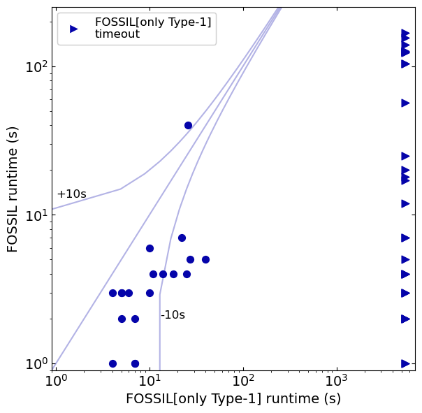

We test the efficacy of counterexamples by removing each kind during synthesis. We do not ablate counterexamples since proposed lemmas would be unrelated to the theorem and a comparison is not meaningful. We perform ablation studies removing both and counterexamples or only removing counterexamples.
Efficacy of and counterexamples:
It is not possible to directly run our synthesis engine without and counterexamples as the same invalid lemmas can be continuously re-proposed. We hence modify our algorithm to perform the ablation study. The algorithm differs from FOSSIL (Figure 2) in two ways. First, the Synthesize module can skip solutions, proceeding to others. Second, when a lemma is not provable (line 16 in Figure 2) we simply discard the lemma by asking the synthesis engine to skip to the next solution. We do this until a valid lemma is found, at which point we move to the outer loop (line 4) and attempt to prove the goal again. Of course, in this algorithm, we also do not maintain sets of or counterexamples and only use the counterexample in the synthesis query.
In our implementation, we integrate a version of FOSSIL with the state-of-the-art SyGuS solver in CVC4 (CVC4Sy), providing only counterexamples during synthesis. We used the efficient streaming mode of CVC4Sy that can skip solutions. This mode generates a stream of solutions to a synthesis query without repetition, and we simply skip along this stream when we reject candidate lemmas. CVC4Sy is well-optimized, performing symmetry and semantic reductions (Reynolds et al. 2019). We used a timeout of 1 hour for the ablated algorithm.
Figure 4(a) compares the ablated tool against our tool (with all types of counterexamples) on Suite #1 benchmarks. Apart from a few outliers where the lemmas proposed are very simple, FOSSIL with only counterexamples performs drastically worse than FOSSIL with all three counterexamples. of the benchmarks did not terminate with the ablated tool before the timeout. This shows the efficacy of and counterexamples in guiding search.
We also perform this experiment with the synthetic benchmarks (Suite #2). FOSSIL using only counterexamples surprisingly solves only 1 out of the 673 benchmarks within 10 minutes. This again demonstrates the efficacy of and counterexamples.
Efficacy of counterexamples
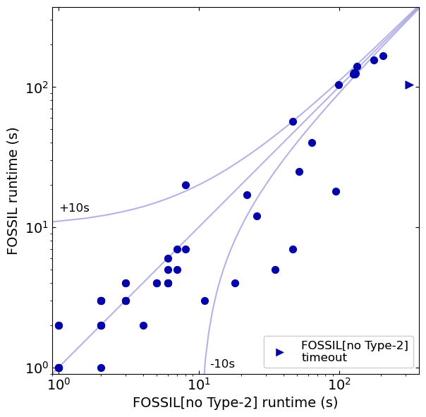
We evaluate the efficacy of countermodels in FOSSIL by building a version of FOSSIL that does not use counterexamples.
The ablated algorithm is similar to the one in Figure 2 except for the case where a lemma is not provable (line 16). If a lemma cannot be proven valid, we do not try to generate a counterexample (lines 17- 19) and skip directly to generating a counterexample (line 21). A counterexample can always be generated since it witnesses the non-provability of a lemma (see Section 3.2). It also ensures that such unprovable lemmas will not be re-proposed.
Figure 4(b) shows the running time comparison between the FOSSIL tool and the FOSSIL tool without counterexamples. The ablated tool does not solve one of the benchmarks and is slower in general for many benchmarks, especially those that require more than 10 seconds to solve. countermodels seem to have a higher impact in pruning the search space for more complex theorems. Figure 5 shows a comparison in the number of proposed lemmas for FOSSIL vs. FOSSIL without counterexample models. Fewer lemmas are proposed for most benchmarks in the FOSSIL tool, showing the efficacy of the guidance of counterexamples.
6.6. RQ3: Comparison with CVC4 SyGuS Solver
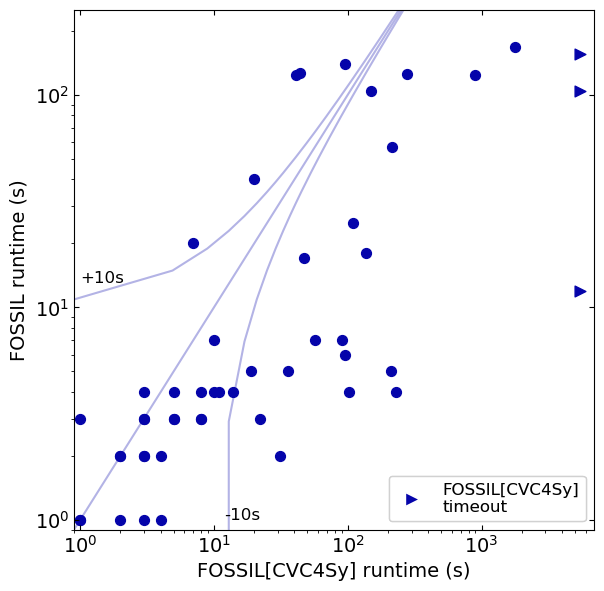
To evaluate the efficacy of our custom synthesis tool that learns from first-order models with grounded constraint solving, we compare our synthesis tool with CVC4Sy (in standard mode with all counterexamples), utilizing the synthesis engines in an identical fashion to the FOSSIL tool. We use a timeout of 1 hour for the ablated algorithm. Figure 4(c) shows the results of this evaluation and indicates that as theorems become more complex, FOSSIL with our custom constraint-based synthesis solver solidly outperforms FOSSIL with CVC4Sy as the synthesis solver. Thus, exploiting the form of synthesis in this domain that has ground constraints is useful.
6.7. Comparison with ADT/Separation Logic Tools
The idea of discovering inductive hypotheses to prove theorems is a problem that has been studied in many logical contexts. We are not aware of any tools that synthesize inductive lemmas for FO+lfp, especially ones that can handle foreground and background sorts as in our setting.
Comparing tools that work for different logics (FO+lfp, algebraic datatypes, separation logic) is inherently hard and poses several challenges: the logics being different, the hardness of translating theorems between them, translation bloat, translations that make theorems harder and required lemmas more complex, tools supporting only restricted fragments, and so on. These make fair comparisons hard.
In this section however, we attempt to compare our tool with tools for algebraic datatypes (ADTs) and separation logic on our benchmarks, making the best translation effort. Though our tool performs much better than these tools on our benchmarks, this should not be construed as evidence that the other tools are inferior in their native settings. Yet, as the comparison below will show, solving theorems in FO+lfp effectively by reducing them to tools for other logics does not seem possible. We also believe that incorporating our ideas into lemma synthesis tools for these logics natively is an interesting future direction.
Comparison with Tools for Algebraic Datatypes
Theoretically, the logic FO+lfp and FO logic over algebraic datatypes are very different. In pure ADT logics, the universe is a single universe while FO+lfp admits a multitude of universes. Furthermore, our benchmarks are motivated by reasoning over pointer-based heaps that embed data structures, which are different from pure mathematical algebraic datatypes (heaps admit a spaghetti of pointers that embed overlapping data structures). Consequently, we find it impossible to encode our benchmarks in a pure ADT logic.
However, when a first-order logic over ADTs includes uninterpreted functions (or higher-order functions), we can find reasonable encodings. We can model locations using elements of some ADT (say with succ) or even a background theory of integers if supported. We can model pointers using uninterpreted functions from locations to locations. Least fixpoint definitions can be modeled in several ways. We choose one that does not involve specific background sorts (such as true natural numbers) and instead uses the structure of ADTs.
We encode finite pointer-linked data structures such as linked lists and linked trees using ADTs such as lists and trees, respectively, that store locations constituting the linked data structure. Now, recursive definitions on ADTs can capture whether a list/tree of locations corresponds to a linked list/tree by checking, recursively, that the relevant pointers (, or ) relate the locations stored in the ADT correctly. Using a mild generalization of this technique, we can encode recursively defined data structures of all kinds used in our benchmarks (including list segments, cyclic lists, doubly linked lists, binary search trees, etc.) in a fairly natural way.
We encoded all 50 benchmarks from Suite #1 into CVC4+ig (Reynolds and Kuncak 2015) and ADTInd (Yang et al. 2019), both of which use induction and lemma synthesis. CVC4+ig solved 1/50 benchmarks, and ADTInd solved 8/50 benchmarks within 15 minutes. This demonstrates that our tool performs significantly better on our benchmarks than reductions to these tools do.
Comparison with Separation Logic Tools
We consider tools in the Separation Logic Competition (SL-COMP) (Sighireanu et al. 2019) (note that these tools do not have grammars for lemmas).
There are many restrictions imposed by the various divisions and tools that make encoding our benchmarks challenging. None of the tools for the closest division qf_shid_entl support conjunction of heap formulas that we require to encode our benchmarks. Also, some of our benchmarks mention heaplets explicitly and thus are hard to encode.
We consider the solver SLS (Songbird+Lemma Synthesis) (Ta et al. 2017) that won the 2019 SL-COMP competition for the qf_shid_entl division. SLS has support for synthesizing inductive lemmas. As mentioned above, many of our examples cannot be translated faithfully into SLS. We were able to encode and prove valid 14 of the 50 examples from Suite #1. There were several examples that we could encode but which SLS was unable to prove (at least 8 such: cyclic-next, list-even-or-odd, and the 6 program reachability examples).
7. Related Work
Quantifier Instantiation. Quantifier instantiation is a common tool for reasoning using SMT solvers (Reynolds 2017). E-matching is an instantiation technique used in the Simplify theorem prover (Detlefs et al. 2005), which chooses instantiations based on matching pattern terms. Similar methods are implemented in other SMT solvers (Barrett et al. 2011; de Moura and Bjørner 2008; Rümmer 2012), as well as methods for combining term instantiation with background SMT solvers (Ge and de Moura 2009). The work in (Feldman et al. 2017) considers bounded quantifier instantiation in a pure FO setting (EPR) without background theories.
Natural Proofs. Our work directly builds off work related to natural proofs (Madhusudan et al. 2012; Qiu et al. 2013; Pek et al. 2014; Suter et al. 2010; Löding et al. 2018). VCs similar to the theorems in our experiments are present in (Qiu et al. 2013), though lemmas needed to be user-provided. Work in (Löding et al. 2018) provided foundations for the work on natural proofs that preceded it. Completeness results in (Löding et al. 2018) directly contribute to our completeness results in this paper, and the techniques outlined in (Löding et al. 2018) are directly implemented in our tool.
Reasoning with Recursive Definitions. There is vast literature on reasoning with recursive definitions. The NQTHM prover developed by Boyer and Moore (Boyer and Moore 1988) and its successor ACL2 (Kaufmann and Moore 1997; Kaufmann et al. 2000) had support for recursive functions and had several induction heuristics to find inductive proofs. Recent works on cyclic proofs (Brotherston et al. 2011; Ta et al. 2016) also use heuristics for reasoning about recursive definitions. Additionally, an ongoing area of research involves decidable logics for recursive data structures (Le et al. 2017). Naturally, the expressive power of these logics is restricted in order to obtain a decidable validity problem. Further techniques in Dafny (Leino 2012) and Verifast (Jacobs et al. 2011) allow for verification via unfolding (or folding) recursive definitions, potentially based on user suggestions. These are instances of “unfold-and-match” (Madhusudan et al. 2012; Nguyen and Chin 2008; Pek et al. 2014; Qiu et al. 2013; Suter et al. 2010), a common heuristic for reasoning with recursive definitions that involves unfolding a recursive definition a few times and finding a proof of validity with the unfolded formulas, treating recursive definitions as uninterpreted.
Lemma Synthesis. The work in (Chu et al. 2015) uses proof-theoretic techniques to discover subgoals during proofs that serve as inductive hypotheses to help the proof. This relies on chancing upon inductive lemmas during proof, and the paper does not provide any relative completeness results. In contrast, our technique is syntax-guided for arbitrary lemmas and is relatively complete. Other lemma synthesis approaches include that of the work in (Zhang et al. 2021), which also uses SyGuS for lemma generation, but operates over the simpler domain of bitvector problems. SLS (Songbird+Lemma Synthesis) (Ta et al. 2016) is a tool for lemma synthesis over Separation Logic. SLS identifies candidate lemma templates by looking at the heap structure of a given entailment. It then conducts structural induction proofs to generate constraints on top of a lemma template, then solves the constraints to refine the template and discover inductive lemmas. SLS only supports a constrained version of SL, disallowing, for example, conjunctions of heap formulas. As a result, many FO+lfp formulas are inexpressible. Refer to Section 6.7 for a detailed comparison between FOSSIL and SLS on our set of benchmarks.
Formula Synthesis. The problem of synthesizing or learning first-order formulas from first-order models has seen recent development. In this space, our synthesis technique is specialized; we only learn universally quantified prenex formulas and hence use a mechanism that synthesizes the quantifier-free matrix using constraints that implicitly assume universal quantification. The work in (Krogmeier and Madhusudan 2022) tackles the harder problem of synthesizing formulas with unboundedly many quantifiers but over finitely many variables (possibly reusing variables) and proves decidability results using tree automata. However, they do not present any practically effective algorithms, and naive implementations of tree automata techniques suffer from state-space explosion. The work in (Koenig et al. 2020) develops a synthesis technique that reduces to SAT, but does not handle grammars; therefore, whether the technique can be used in our work is unclear. Further, whether either of these two works can be extended to effectively synthesize formulas involving background theories like integers and sets, which we require in FOSSIL, is also unclear.
ICE Learning. Our counterexamples and framework bear resemblance to the work on ICE Learning (Garg et al. 2014) for invariant synthesis, as invariants in imperative program verification are similar to inductive hypotheses. FOSSIL cannot handle invariant synthesis problems, however, despite the fact that inductive invariants are similar to inductive lemmas when programs are written as FO+lfp formulae. This is because we do not synthesize lemmas that quantify over background sorts such as integers (this distinction also applies to other methods catering to loop invariant synthesis (Neider et al. 2018), and as such we do not compare with such works). Our synthesis algorithm that uses essentially Boolean constraint solving exploits the fact that expressions synthesized do not have constants over the background sort. Second, while negative counterexamples in ICE correspond roughly to models (though the latter are non-provability counterexamples, similar to (Neider et al. 2018)), the positive and implication counterexamples in ICE do not seem to have a strict counterpart in our framework. However, counterexamples come close to implication counterexamples. In the ICE setting programs change configurations, leading to implication counterexamples. In contrast, in the pure FO+lfp theorem proving setting, there are no changes to models that call for having two separate models as in an implication counterexample. However, models are a single positive counterexample over which the PFP of a lemma must hold. The PFP formula is itself an implication where the lemma to be synthesized “appears” on both sides, which makes them similar in spirit to implication counterexamples in ICE.
ADTs and Term Algebras. Turning to related work in proving properties of term algebras and algebraic datatypes (ADTs), the work in (Kovács et al. 2017) focuses on automating logics over arbitrary term algebras using FO approximations. For lemma synthesis, the work in (Yang et al. 2019) is another effort to synthesize inductive lemmas and also uses SyGuS (but without counterexample-guidance). The work in (Reynolds and Kuncak 2015) also aims to synthesize inductive lemmas, and we provide a detailed comparison with this work in Section 6.7. The work in (Govind V K et al. 2022) infers lemmas for synthesizing invariants but does not use counterexamples.
We emphasize again, however, that work on ADTs/term algebras and our work here on FO+lfp are very different and hard to compare both theoretically and experimentally. First, a term algebra universe (ADTs) (without background universe) is a single universe/model (with fixed interpretation of functions such as constructors/destructors) that is negation-complete. Our universes model heaps and admit a multitude of universes. Second, the universe of a term algebra has a complete recursive axiomatization (Mal’tsev 1962; Hodges 1997), and hence FO properties of ADTs are in fact decidable, while FO+lfp does not even admit complete procedures, let alone decidable ones. Third, several data structures we work with do not even have analogous structures in the ADT world— e.g., list segments between two locations, doubly-linked lists, cyclic lists. And destructive pointer updates on them are not expressible in the world of ADTs. Also defining data structures common in ADTs in the heap world are considerably more difficult, as we need to express separation (for example, even the definition of a tree requires such separation constraints; see Section 2). Consequently, a fair experimental comparison of our tools against those developed for ADTs (Sonnex et al. 2012; Cruanes 2017; Hajdú et al. 2020; Boyer and Moore 1988; Kaufmann and Moore 1997; Passmore et al. 2020; Claessen et al. 2013; Johansson 2019; Govind V K et al. 2022) is difficult. Still, when the logic admits uninterpreted or higher-order functions, an encoding is possible (Section 6.7). Extending our techniques to build a lemma synthesis technique/tool with built-in support for ADTs, especially to reason with functional programs, is an interesting future direction.
8. Conclusions
The primary contribution of this paper is an inductive lemma synthesis technique for FO+lfp with background theories that learns from semantically-rich counterexample FO models that witness non-provabilitySuch a search for inductive lemmas based on the semantics of theorems/lemmas can be useful in other contexts— e.g, in identifying lemmas from a large corpus to help prove theorems. For instance, the work in (Bansal et al. 2019) uses machine learning to find proofs, but currently little semantic information is used in learning. Extending our work to synthesizing lemmas for other logics, especially over ADTs (see Section 7) as well as Separation Logic is also interesting. We also believe that building general lemma synthesis engines that extend SMT solvers can be valuable for researchers who use automated theorem proving in a variety of application domains.
Data Availability Statement
The code and data artifacts required to reproduce the experiments on the FOSSIL tool and various ablation studies are available via ACM DL at (Murali et al. 2022).
Acknowledgments
This work is supported in part by a research grant from Amazon and a Discovery Partners Institute (DPI) science team seed grant.
References
- (1)
- Alur et al. (2015) Rajeev Alur, Rastislav Bodík, Eric Dallal, Dana Fisman, Pranav Garg, Garvit Juniwal, Hadas Kress-Gazit, P. Madhusudan, Milo M. K. Martin, Mukund Raghothaman, Shambwaditya Saha, Sanjit A. Seshia, Rishabh Singh, Armando Solar-Lezama, Emina Torlak, and Abhishek Udupa. 2015. Syntax-Guided Synthesis. IOS Press, 1–25. https://doi.org/10.3233/978-1-61499-495-4-1
- Alur et al. (2018) Rajeev Alur, Rishabh Singh, Dana Fisman, and Armando Solar-Lezama. 2018. Search-Based Program Synthesis. Commun. ACM 61, 12 (Nov. 2018), 84–93. https://doi.org/10.1145/3208071
- Ball and Rajamani (2002) Thomas Ball and Sriram K. Rajamani. 2002. The SLAM Project: Debugging System Software via Static Analysis. (2002), 1–3. https://doi.org/10.1145/503272.503274
- Bansal et al. (2019) Kshitij Bansal, Sarah M. Loos, Markus N. Rabe, Christian Szegedy, and Stewart Wilcox. 2019. HOList: An Environment for Machine Learning of Higher-Order Theorem Proving. https://doi.org/10.48550/ARXIV.1904.03241
- Barrett et al. (2011) Clark Barrett, Christopher L. Conway, Morgan Deters, Liana Hadarean, Dejan Jovanović, Tim King, Andrew Reynolds, and Cesare Tinelli. 2011. CVC4. In Computer Aided Verification, Ganesh Gopalakrishnan and Shaz Qadeer (Eds.). Springer Berlin Heidelberg, Berlin, Heidelberg, 171–177. https://doi.org/10.1007/978-3-642-22110-1_14
- Boyer and Moore (1988) Robert S. Boyer and J. Strother Moore. 1988. A Computational Logic Handbook. Academic Press Professional, Inc., USA.
- Bradley and Manna (2007) Aaron R. Bradley and Zohar Manna. 2007. The Calculus of Computation: Decision Procedures with Applications to Verification. Springer-Verlag, Berlin, Heidelberg. https://doi.org/10.1007/978-3-540-74113-8
- Brotherston et al. (2011) James Brotherston, Dino Distefano, and Rasmus Lerchedahl Petersen. 2011. Automated Cyclic Entailment Proofs in Separation Logic. In Automated Deduction – CADE-23, Nikolaj Bjørner and Viorica Sofronie-Stokkermans (Eds.). Springer Berlin Heidelberg, Berlin, Heidelberg, 131–146. https://doi.org/10.1007/978-3-642-22438-6_12
- Calcagno et al. (2005) Cristiano Calcagno, Philippa Gardner, and Matthew Hague. 2005. From Separation Logic to First-Order Logic. In Foundations of Software Science and Computational Structures, Vladimiro Sassone (Ed.). Springer Berlin Heidelberg, Berlin, Heidelberg, 395–409. https://doi.org/10.1007/978-3-540-31982-5_25
- Chu et al. (2015) Duc-Hiep Chu, Joxan Jaffar, and Minh-Thai Trinh. 2015. Automatic Induction Proofs of Data-Structures in Imperative Programs. In Proceedings of the 36th ACM SIGPLAN Conference on Programming Language Design and Implementation (Portland, OR, USA) (PLDI ’15). Association for Computing Machinery, New York, NY, USA, 457–466. https://doi.org/10.1145/2737924.2737984
- Claessen et al. (2013) Koen Claessen, Moa Johansson, Dan Rosén, and Nicholas Smallbone. 2013. Automating Inductive Proofs Using Theory Exploration. In Automated Deduction - CADE-24 - 24th International Conference on Automated Deduction, Lake Placid, NY, USA, June 9-14, 2013. Proceedings (Lecture Notes in Computer Science, Vol. 7898), Maria Paola Bonacina (Ed.). Springer, 392–406. https://doi.org/10.1007/978-3-642-38574-2_27
- Cruanes (2017) Simon Cruanes. 2017. Superposition with Structural Induction. In Frontiers of Combining Systems, Clare Dixon and Marcelo Finger (Eds.). Springer International Publishing, Cham, 172–188. https://doi.org/10.1007/978-3-319-66167-4_10
- de Moura and Bjørner (2008) Leonardo de Moura and Nikolaj Bjørner. 2008. Z3: An Efficient SMT Solver. In Tools and Algorithms for the Construction and Analysis of Systems, C. R. Ramakrishnan and Jakob Rehof (Eds.). Springer Berlin Heidelberg, Berlin, Heidelberg, 337–340. https://doi.org/10.1007/978-3-540-78800-3_24
- Detlefs et al. (2005) David Detlefs, Greg Nelson, and James B. Saxe. 2005. Simplify: A Theorem Prover for Program Checking. J. ACM 52, 3 (May 2005), 365–473. https://doi.org/10.1145/1066100.1066102
- Enderton (2001) H.B. Enderton. 2001. A Mathematical Introduction to Logic. Elsevier Science Publishers Ltd. https://doi.org/10.1016/C2009-0-22107-6
- Feldman et al. (2017) Yotam M. Y. Feldman, Oded Padon, Neil Immerman, Mooly Sagiv, and Sharon Shoham. 2017. Bounded Quantifier Instantiation for Checking Inductive Invariants. In Tools and Algorithms for the Construction and Analysis of Systems, Axel Legay and Tiziana Margaria (Eds.). Springer Berlin Heidelberg, Berlin, Heidelberg, 76–95. https://doi.org/10.1007/978-3-662-54577-5_5
- Garg et al. (2014) Pranav Garg, Christof Löding, P. Madhusudan, and Daniel Neider. 2014. ICE: A Robust Framework for Learning Invariants. In Computer Aided Verification, Armin Biere and Roderick Bloem (Eds.). Springer International Publishing, Cham, 69–87. https://doi.org/10.1007/978-3-319-08867-9_5
- Ge and de Moura (2009) Yeting Ge and Leonardo de Moura. 2009. Complete Instantiation for Quantified Formulas in Satisfiabiliby Modulo Theories. In Computer Aided Verification, Ahmed Bouajjani and Oded Maler (Eds.). Springer Berlin Heidelberg, Berlin, Heidelberg, 306–320. https://doi.org/10.1007/978-3-642-02658-4_25
- Govind V K et al. (2022) Hari Govind V K, Sharon Shoham, and Arie Gurfinkel. 2022. Solving Constrained Horn Clauses modulo Algebraic Data Types and Recursive Functions. Proc. ACM Program. Lang. 6, POPL, Article 60 (Jan 2022), 29 pages. https://doi.org/10.1145/3498722
- Grädel et al. (2007) Erich Grädel, Phokion G. Kolaitis, Leonid Libkin, Maarten Marx, Joel Spencer, Moshe Y. Vardi, Yde Venema, and Scott Weinstein. 2007. Finite Model Theory and Its Applications. Springer. https://doi.org/10.1007/3-540-68804-8
- Hajdú et al. (2020) Márton Hajdú, Petra Hozzová, Laura Kovács, Johannes Schoisswohl, and Andrei Voronkov. 2020. Induction with Generalization in Superposition Reasoning. In Intelligent Computer Mathematics - 13th International Conference, CICM 2020, Bertinoro, Italy, July 26-31, 2020, Proceedings (Lecture Notes in Computer Science, Vol. 12236), Christoph Benzmüller and Bruce R. Miller (Eds.). Springer, 123–137. https://doi.org/10.1007/978-3-030-53518-6_8
- Hodges (1997) Wilfrid Hodges. 1997. A Shorter Model Theory. Cambridge University Press, USA.
- Jacobs et al. (2011) Bart Jacobs, Jan Smans, Pieter Philippaerts, Frédéric Vogels, Willem Penninckx, and Frank Piessens. 2011. VeriFast: A Powerful, Sound, Predictable, Fast Verifier for C and Java. In NASA Formal Methods, Mihaela Bobaru, Klaus Havelund, Gerard J. Holzmann, and Rajeev Joshi (Eds.). Springer Berlin Heidelberg, Berlin, Heidelberg, 41–55. https://doi.org/10.1007/978-3-642-20398-5_4
- Johansson (2019) Moa Johansson. 2019. Lemma Discovery for Induction - A Survey. In Intelligent Computer Mathematics - 12th International Conference, CICM 2019, Prague, Czech Republic, July 8-12, 2019, Proceedings (Lecture Notes in Computer Science, Vol. 11617), Cezary Kaliszyk, Edwin C. Brady, Andrea Kohlhase, and Claudio Sacerdoti Coen (Eds.). Springer, 125–139. https://doi.org/10.1007/978-3-030-23250-4_9
- Kaufmann and Moore (1997) Matt Kaufmann and J. S. Moore. 1997. An Industrial Strength Theorem Prover for a Logic Based on Common Lisp. IEEE Trans. Softw. Eng. 23, 4 (April 1997), 203–213. https://doi.org/10.1109/32.588534
- Kaufmann et al. (2000) Matt Kaufmann, J. Strother Moore, and Panagiotis Manolios. 2000. Computer-Aided Reasoning: An Approach. Springer New York, NY. https://doi.org/10.1007/978-1-4615-4449-4
- Koenig et al. (2020) Jason R. Koenig, Oded Padon, Neil Immerman, and Alex Aiken. 2020. First-Order Quantified Separators. In Proceedings of the 41st ACM SIGPLAN Conference on Programming Language Design and Implementation (London, UK) (PLDI 2020). Association for Computing Machinery, New York, NY, USA, 703–717. https://doi.org/10.1145/3385412.3386018
- Kovács et al. (2017) Laura Kovács, Simon Robillard, and Andrei Voronkov. 2017. Coming to Terms with Quantified Reasoning. In Proceedings of the 44th ACM SIGPLAN Symposium on Principles of Programming Languages (Paris, France) (POPL ’17). ACM, New York, NY, USA, 260–270. https://doi.org/10.1145/3009837.3009887
- Krogmeier and Madhusudan (2022) Paul Krogmeier and P. Madhusudan. 2022. Learning Formulas in Finite Variable Logics. Proc. ACM Program. Lang. 6, POPL, Article 10 (Jan 2022), 28 pages. https://doi.org/10.1145/3498671
- Le et al. (2017) Quang Loc Le, Makoto Tatsuta, Jun Sun, and Wei-Ngan Chin. 2017. A Decidable Fragment in Separation Logic with Inductive Predicates and Arithmetic. In Computer Aided Verification, Rupak Majumdar and Viktor Kunčak (Eds.). Springer International Publishing, Cham, 495–517. https://doi.org/10.1007/978-3-319-63390-9_26
- Leino (2012) K. Rustan M. Leino. 2012. Automating Induction with an SMT Solver. In Proceedings of the 13th International Conference on Verification, Model Checking, and Abstract Interpretation (Philadelphia, PA) (VMCAI’12). Springer-Verlag, Berlin, Heidelberg, 315–331. https://doi.org/10.1007/978-3-642-27940-9_21
- Libkin (2004) Leonid Libkin. 2004. Elements of Finite Model Theory. Springer Berlin, Heidelberg. https://doi.org/10.1007/978-3-662-07003-1
- Löding et al. (2018) Christof Löding, P. Madhusudan, and Lucas Peña. 2018. Foundations for natural proofs and quantifier instantiation. PACMPL 2, POPL (2018), 10:1–10:30. https://doi.org/10.1145/3158098
- Madhusudan et al. (2012) P. Madhusudan, Xiaokang Qiu, and Andrei Ştefănescu. 2012. Recursive Proofs for Inductive Tree Data-structures. In Proceedings of the 39th Annual ACM SIGPLAN-SIGACT Symposium on Principles of Programming Languages (Philadelphia, PA, USA) (POPL ’12). ACM, New York, NY, USA, 123–136. https://doi.org/10.1145/2103656.2103673
- Mal’tsev (1962) A. I. Mal’tsev. 1962. Axiomatizable classes of locally free algebras of certain types. Sibirsk. Mat. Zh. 3 (1962), 729–743. Issue 5. http://mi.mathnet.ru/eng/smj/v3/i5/p729
- Murali et al. (2022) Adithya Murali, Lucas Peña, Eion Blanchard, Christof Löding, and P. Madhusudan. 2022. Artifact for OOPSLA 2022 Article Model-Guided Synthesis of Inductive Lemmas for FOL with Least Fixpoints. https://doi.org/10.1145/3554331
- Murali et al. (2020) Adithya Murali, Lucas Peña, Christof Löding, and P. Madhusudan. 2020. A First-Order Logic with Frames. In Programming Languages and Systems, Peter Müller (Ed.). Springer International Publishing, Cham, 515–543. https://doi.org/10.1007/978-3-030-44914-8_19
- Namjoshi and Kurshan (2000) Kedar S. Namjoshi and Robert P. Kurshan. 2000. Syntactic Program Transformations for Automatic Abstraction. In Computer Aided Verification, E. Allen Emerson and Aravinda Prasad Sistla (Eds.). Springer Berlin Heidelberg, Berlin, Heidelberg, 435–449. https://doi.org/10.1007/10722167_33
- Neider et al. (2018) Daniel Neider, Pranav Garg, P. Madhusudan, Shambwaditya Saha, and Daejun Park. 2018. Invariant Synthesis for Incomplete Verification Engines. In Tools and Algorithms for the Construction and Analysis of Systems, Dirk Beyer and Marieke Huisman (Eds.). Springer International Publishing, Cham, 232–250. https://doi.org/10.1007/978-3-319-89960-2_13
- Nelson (1980) Charles Gregory Nelson. 1980. Techniques for Program Verification. Ph. D. Dissertation. Stanford University, Stanford, CA, USA. AAI8011683.
- Nelson and Oppen (1979) Greg Nelson and Derek C. Oppen. 1979. Simplification by Cooperating Decision Procedures. ACM Trans. Program. Lang. Syst. 1, 2 (Oct 1979), 245–257. https://doi.org/10.1145/357073.357079
- Nguyen and Chin (2008) Huu Hai Nguyen and Wei-Ngan Chin. 2008. Enhancing Program Verification with Lemmas. In Proceedings of the 20th International Conference on Computer Aided Verification (Princeton, NJ, USA) (CAV ’08). Springer-Verlag, Berlin, Heidelberg, 355–369. https://doi.org/10.1007/978-3-540-70545-1_34
- Passmore et al. (2020) Grant Passmore, Simon Cruanes, Denis Ignatovich, Dave Aitken, Matt Bray, Elijah Kagan, Kostya Kanishev, Ewen Maclean, and Nicola Mometto. 2020. The Imandra Automated Reasoning System (System Description). In Automated Reasoning, Nicolas Peltier and Viorica Sofronie-Stokkermans (Eds.). Springer International Publishing, Cham, 464–471. https://doi.org/10.1007/978-3-030-51054-1_30
- Pek et al. (2014) Edgar Pek, Xiaokang Qiu, and P. Madhusudan. 2014. Natural Proofs for Data Structure Manipulation in C Using Separation Logic. In Proceedings of the 35th ACM SIGPLAN Conference on Programming Language Design and Implementation (Edinburgh, United Kingdom) (PLDI ’14). ACM, New York, NY, USA, 440–451. https://doi.org/10.1145/2594291.2594325
- Qiu et al. (2013) Xiaokang Qiu, Pranav Garg, Andrei Ştefănescu, and P. Madhusudan. 2013. Natural Proofs for Structure, Data, and Separation. In Proceedings of the 34th ACM SIGPLAN Conference on Programming Language Design and Implementation (Seattle, Washington, USA) (PLDI ’13). ACM, New York, NY, USA, 231–242. https://doi.org/10.1145/2491956.2462169
- Reynolds (2017) Andrew Reynolds. 2017. Conflicts, Models and Heuristics for Quantifier Instantiation in SMT. In Vampire 2016. Proceedings of the 3rd Vampire Workshop (EPiC Series in Computing, Vol. 44), Laura Kovacs and Andrei Voronkov (Eds.). EasyChair, 1–15. https://doi.org/10.29007/jmd3
- Reynolds et al. (2019) Andrew Reynolds, Haniel Barbosa, Andres Nötzli, Clark Barrett, and Cesare Tinelli. 2019. cvc4sy: Smart and Fast Term Enumeration for Syntax-Guided Synthesis. In Computer Aided Verification, Isil Dillig and Serdar Tasiran (Eds.). Springer International Publishing, Cham, 74–83. https://doi.org/10.1007/978-3-030-25543-5_5
- Reynolds and Kuncak (2015) Andrew Reynolds and Viktor Kuncak. 2015. Induction for SMT Solvers. In Verification, Model Checking, and Abstract Interpretation, Deepak D’Souza, Akash Lal, and Kim Guldstrand Larsen (Eds.). Springer Berlin Heidelberg, Berlin, Heidelberg, 80–98. https://doi.org/10.1007/978-3-662-46081-8_5
- Reynolds (2002) John C. Reynolds. 2002. Separation Logic: A Logic for Shared Mutable Data Structures. In Proceedings of the 17th Annual IEEE Symposium on Logic in Computer Science (LICS ’02). IEEE Press, 55–74. https://doi.org/10.1109/LICS.2002.1029817
- Rümmer (2012) Philipp Rümmer. 2012. E-Matching with Free Variables. In Logic for Programming, Artificial Intelligence, and Reasoning, Nikolaj Bjørner and Andrei Voronkov (Eds.). Springer Berlin Heidelberg, Berlin, Heidelberg, 359–374. https://doi.org/10.1007/978-3-642-28717-6_28
- Sighireanu et al. (2019) Mihaela Sighireanu, Juan A. Navarro Pérez, Andrey Rybalchenko, Nikos Gorogiannis, Radu Iosif, Andrew Reynolds, Cristina Serban, Jens Katelaan, Christoph Matheja, Thomas Noll, Florian Zuleger, Wei-Ngan Chin, Quang Loc Le, Quang-Trung Ta, Ton-Chanh Le, Thanh-Toan Nguyen, Siau-Cheng Khoo, Michal Cyprian, Adam Rogalewicz, Tomas Vojnar, Constantin Enea, Ondrej Lengal, Chong Gao, and Zhilin Wu. 2019. SL-COMP: Competition of Solvers for Separation Logic. In Tools and Algorithms for the Construction and Analysis of Systems, Dirk Beyer, Marieke Huisman, Fabrice Kordon, and Bernhard Steffen (Eds.). Springer International Publishing, Cham, 116–132. https://doi.org/10.1007/978-3-030-17502-3_8
- Solar Lezama (2008) Armando Solar Lezama. 2008. Program Synthesis By Sketching. Ph. D. Dissertation. EECS Department, University of California, Berkeley. http://www2.eecs.berkeley.edu/Pubs/TechRpts/2008/EECS-2008-177.html
- Solar-Lezama et al. (2007) Armando Solar-Lezama, Gilad Arnold, Liviu Tancau, Rastislav Bodík, Vijay A. Saraswat, and Sanjit A. Seshia. 2007. Sketching stencils. In Proceedings of the ACM SIGPLAN 2007 Conference on Programming Language Design and Implementation, San Diego, California, USA, June 10-13, 2007, Jeanne Ferrante and Kathryn S. McKinley (Eds.). ACM, 167–178. https://doi.org/10.1145/1250734.1250754
- Sonnex et al. (2012) William Sonnex, Sophia Drossopoulou, and Susan Eisenbach. 2012. Zeno: An Automated Prover for Properties of Recursive Data Structures. In Tools and Algorithms for the Construction and Analysis of Systems, Cormac Flanagan and Barbara König (Eds.). Springer Berlin Heidelberg, Berlin, Heidelberg, 407–421. https://doi.org/10.1007/978-3-642-28756-5_28
- Suter et al. (2010) Philippe Suter, Mirco Dotta, and Viktor Kunćak. 2010. Decision Procedures for Algebraic Data Types with Abstractions. In Proceedings of the 37th Annual ACM SIGPLAN-SIGACT Symposium on Principles of Programming Languages (Madrid, Spain) (POPL ’10). ACM, New York, NY, USA, 199–210. https://doi.org/10.1145/1706299.1706325
- Ta et al. (2016) Quang-Trung Ta, Ton Chanh Le, Siau-Cheng Khoo, and Wei-Ngan Chin. 2016. Automated Mutual Explicit Induction Proof in Separation Logic. In FM 2016: Formal Methods, John Fitzgerald, Constance Heitmeyer, Stefania Gnesi, and Anna Philippou (Eds.). Springer International Publishing, Cham, 659–676. https://doi.org/10.1007/978-3-319-48989-6_40
- Ta et al. (2017) Quang-Trung Ta, Ton Chanh Le, Siau-Cheng Khoo, and Wei-Ngan Chin. 2017. Automated Lemma Synthesis in Symbolic-Heap Separation Logic. Proc. ACM Program. Lang. 2, POPL, Article 9 (Dec 2017), 29 pages. https://doi.org/10.1145/3158097
- Tarski (1955) Alfred Tarski. 1955. A lattice-theoretical fixpoint theorem and its applications. Pacific J. Math. 5, 2 (1955), 285 – 309. https://projecteuclid.org/euclid.pjm/1103044538
- Yang et al. (2019) Weikun Yang, Grigory Fedyukovich, and Aarti Gupta. 2019. Lemma Synthesis for Automating Induction over Algebraic Data Types. In Principles and Practice of Constraint Programming, Thomas Schiex and Simon de Givry (Eds.). Springer International Publishing, Cham, 600–617. https://doi.org/10.1007/978-3-030-30048-7_35
- Zhang et al. (2021) Hongce Zhang, Aarti Gupta, and Sharad Malik. 2021. Syntax-Guided Synthesis for Lemma Generation in Hardware Model Checking. In Verification, Model Checking, and Abstract Interpretation - 22nd International Conference, VMCAI 2021, Copenhagen, Denmark, January 17-19, 2021, Proceedings (Lecture Notes in Computer Science, Vol. 12597), Fritz Henglein, Sharon Shoham, and Yakir Vizel (Eds.). Springer, 325–349. https://doi.org/10.1007/978-3-030-67067-2_15
Appendix A Appendix
A.1. Further details for Section 3
Proof of Theorem 5.1.
Proof.
Assume that there exists some set of independent lemmas that proves . Let us fix and to be such that every as well as the goal (given the lemmas) is provable with a depth instantiation, and the maximum height of any of the productions in that yield a lemma is . We claim that FOSSIL with parameters and will terminate having found a sequence of lemmas that prove .
We induct on the number of lemmas in the set. Since the algorithm is sound, if it terminates there is clearly a sequence of lemmas that proves . We establish that either the algorithm will terminate with a proof of the goal, or at least one will be eventually (at some finite time) chosen by the synthesis module, i.e., it cannot be that the algorithm restarts FOSSIL with new parameters in line 9 or runs forever without choosing one of the lemmas . If some is chosen by the synthesis module, since we know by our choice of that is provable with depth instantiation, it will be added to (see line 12) before all the variables are reset, which reduces the problem to discovering at most independent lemmas whereupon we will appeal to the induction on number of lemmas to be discovered.
It is clear from the definition of that is finite for any . Observe from the description of the algorithm in Section 3.3 that in each round the candidate proposal will either: (i) be prevented from being proposed again in the inner loop (line 7) by the addition of a model, or (ii) be prevented from being proposed again permanently during the execution of FOSSIL (with parameters and ) because it was proved valid and added to or it was proved invalid using a model. This eliminates the possibility that the algorithm keeps on proposing lemmas that are not provable. It either finds a provably valid lemma, or it has no further candidate lemmas to propose, and thus would restart the algorithm with new parameters in line 9.
If it finds a valid lemma, the search space for the next round of lemma synthesis is reduced (because the discovered valid lemma will not be proposed anymore). So this can happen only finitely often.
This leaves us with the possibility that the algorithm reaches line 9 without finding a new candidate lemma. In particular, this means that none of the satisfies the constraints in line 8. We show that this cannot be the case, i.e., that at least one satisfies the constraints (and is therefore a viable proposal for the synthesis module).
It is easy to see that each satisfies constraints 8b and 8c since the former constraint is satisfied by any lemma valid in the FO-lfp theory defined by and , and the latter is satisfied by any lemma that is provable by induction at depth . Both of these conditions are true of every . This leaves us with constraint 8a. Assume for the sake of contradiction that no lemma satisfies the constraint, i.e., there is a model (namely the current model) such that for any . This yields that , which contradicts our initial assumption that collectively prove at depth , i.e., is unsatisfiable. Therefore some satisfies the constraint on line 8a and will eventually be proposed, which concludes our proof. ∎
A.2. Lemma Synthesis Algorithms Relatively Complete wrt Sequential Lemmas
In this section we briefly discuss the problem of designing algorithms for sequential lemma synthesis that are also relatively complete wrt sequential lemmas (instead of just being relatively complete wrt independent lemmas as in Theorem 5.1). To do this we must first see why FOSSIL is not already complete for sequential lemmas. They key obstacle is the model that makes the lemma synthesis goal-directed. Consider the following scenario:
Example A.1 (FOSSIL is not complete for sequence of lemmas).
Consider the case where can be proved using a sequence of two lemmas. Let be provable on its own, be provable assuming , and is provable assuming . At the beginning of the algorithm on line 6 in Figure 2, would be false on since it helps prove . But there is nothing that prevents from being true on , so let us suppose that it is true. If that is the case, then might be selected by the algorithm and then quickly dismissed since it cannot be proved valid without . We would then add a counterexample for it on line 22 witnessing that has no inductive proof. However, the model has not changed (we only recompute it when we find a valid lemma) and therefore will never be proposed as well. We cannot guarantee that a proof of will be found by FOSSIL.
We propose three different strategies to address the above issue:
- (1)
The simplest way to achieve the relative completeness is to utilize FOSSIL as described in Figure 2, but eliminate constraints corresponding to models. This eliminates the problem described in Example A.1 where we need to necessarily synthesize lemmas that help prove the goal, and instead reduces the algorithm to only generating lemma proposals and eliminating spurious proposals using and models. This approach has the obvious disadvantage of not being goal-directed and could lead to large execution time for proof if the sequence of lemmas needed consists of large lemmas (by size) and smaller lemmas could be easily eliminated if given the goal.
- (2)
A second approach is to have the algorithm branch into two-subroutines (both branches searched fairly, dovetailing between them) when given a lemma that is unprovable, one assuming that the lemma is valid and other assuming that it is not. We can then pursue each subroutine until we find a proof or reach a contradiction. However, this algorithm could quickly explode in the number of subroutines even with a few unprovable lemmas and likely impractical.
- (3)
We propose a third alternative that generalises FOSSIL. Looking at the Example A.1, it would be useful if we could update to include the failure to prove so that the lemma synthesis is guided towards . What should be the constraint with which we update the model? The updated model could be such that holds (on the instantiated terms), or it could witness that is not inductive, i.e., cannot be proved by induction. However, these two possibilities are precisely those expressed by the induction principle for . Recall the definition from Section 2.3: the induction principle of a lemma is given by where represents the condition that is inductive. Therefore the induction principle captures the two possibilities of either being valid or not inductive. Our third alternative proposal is thus to use the induction principle to address the problem of completeness for sequences of lemmas in an algorithm we call FOSSIL-IP.
FOSSIL-IP
Let us discuss the third strategy in more detail. Simply put, we would like to add the induction principle for any lemmas that we cannot prove to our axioms and retain the rest of the algorithm. In particular, with respect to the algorithm description in Figure 2 we would maintain a set of induction principles starting out with an empty set and include it in the construction of and on lines 3 and 10. Then, given a proposal that we can neither prove nor establish as being invalid using a model (line 20), we would eliminate falling back to a model on lines 21 and 22 and replace it with the update of with the induction principle of . This algorithm, which we call FOSSIL-IP, is relatively complete for the problem of sequential lemma synthesis:
Theorem A.2 (Relative completeness of FOSSIL-IP wrt sequential lemmas).
If is provable from and by a finite sequence of inductive lemmas, then there is an instantiation depth and grammar height such that FOSSIL-IP terminates and returns a set of lemmas and a set of induction principles proving .
We detail the formulation of proving a theorem using induction principles in Appendix A.2.1. Admittedly, our solution could still create large synthesis queries that could be difficult to handle and therefore has potential disadvantages as do the other two strategies.
A.2.1. Discussion about induction principles and description of FOSSIL-IP
As illustrated in Example A.1, we cannot guarantee that FOSSIL finds a sequence of inductive lemmas proving the goal if such a sequence exists. We need the stronger assumption that a set of independent lemmas exists for proving the goal.
The algorithm FOSSIL-IP is a modification of FOSSIL that is guaranteed to find a proof of the goal if it can be proven by a sequence of inductive lemmas. In addition to the sequence of valid lemmas that is constructed in a similar way as FOSSIL does, FOSSIL-IP additionally uses induction principles of lemmas for which it does not find an inductive proof. It might happen that these induction principles help proving without the algorithm being able to prove the actual lemmas valid. We illustrate the difference between induction principles and lemmas proving for an (artificial) example situation.
Example A.3.
Consider the definition of list from above. Add two constants to the signature, and two recursive definitions and :
So both are defined as list with the only difference that the recursion stops at for if , and for if .
Take . This is certainly true in LFP semantics because if , then is the same as list, otherwise is the same as list. Consider the lemmas and . For each lemma, there are clearly LFP models in which the lemma does not hold (if and , then is false, similarly for ). However, we have that because on each model either or is satisfied.
This illustrates that provability by induction principles does not yield provability by the corresponding lemmas. The other direction, however, is always true, as stated in the following lemma.
Lemma A.4.
If is a sequence of inductive lemmas that prove then the set proves .
Proof.
If does not prove , then there is a model of (in the FO semantics). Since the lemmas from the sequence prove , one of the lemmas has to be false on . Since is true on , we obtain that is false on . If is the smallest index such that is false on , then we get a contradiction to the fact that is an inductive sequence of lemmas, and hence . ∎
| Theorem | Valid Lemmas |
| dlist-list | |
| slist-list | |
| sdlist-dlist | |
| sdlist-dlist-slist | |
| listlen-list | |
| even-list | |
| odd-list | |
| list-even-or-odd | |
| lseg-list | |
| lseg-next | |
| lseg-next-dyn | |
| lseg-trans | |
| lseg-trans2 | |
| lseg-ext | |
| lseg-nil-list | |
| slseg-nil-slist | |
| list-hlist-list | |
| list-hlist-lseg | |
| list-lseg-keys | |
| list-lseg-keys2 | |
| rlist-list | |
| rlist-black-height | |
| rlist-red-height | |
| cyclic-next | |
| tree-dag | |
| bst-tree | |
| maxheap-dag | |
| maxheap-tree | |
| tree-p-tree |
| Theorem | Valid Lemmas |
| tree-p-reach | |
| tree-p-reach-tree | |
| tree-reach | |
| tree-reach2 | |
| dag-reach | |
| dag-reach2 | |
| reach-left-right | |
| bst-left | |
| bst-right | |
| bst-leftmost | |
| bst-left-right | |
| bst-maximal | |
| bst-minimal | |
| maxheap-htree-key | |
| maxheap-keys | |
| reachability | |
| reachability2 | |
| reachability3 | |
| reachability4 | |
| reachability5 | |
| reachability6 |