NeuroDiff: Scalable Differential Verification of Neural Networks using Fine-Grained ApproximationConference: 35th IEEE/ACM International Conference on Automated Software Engineering; September 21–25, 2020; Virtual Event, Australia35th IEEE/ACM International Conference on Automated Software Engineering (ASE ’20), September 21–25, 2020, Virtual Event, AustraliaPrice: 15.00DOI: 10.1145/3324884.3416560ISBN: 978-1-4503-6768-4/20/09
Abstract.
As neural networks make their way into safety-critical systems, where misbehavior can lead to catastrophes, there is a growing interest in certifying the equivalence of two structurally similar neural networks – a problem known as differential verification. For example, compression techniques are often used in practice for deploying trained neural networks on computationally- and energy-constrained devices, which raises the question of how faithfully the compressed network mimics the original network. Unfortunately, existing methods either focus on verifying a single network or rely on loose approximations to prove the equivalence of two networks. Due to overly conservative approximation, differential verification lacks scalability in terms of both accuracy and computational cost. To overcome these problems, we propose NeuroDiff, a symbolic and fine-grained approximation technique that drastically increases the accuracy of differential verification on feed-forward ReLU networks while achieving many orders-of-magnitude speedup. NeuroDiff has two key contributions. The first one is new convex approximations that more accurately bound the difference of two networks under all possible inputs. The second one is judicious use of symbolic variables to represent neurons whose difference bounds have accumulated significant error. We find that these two techniques are complementary, i.e., when combined, the benefit is greater than the sum of their individual benefits. We have evaluated NeuroDiff on a variety of differential verification tasks. Our results show that NeuroDiff is up to 1000X faster and 5X more accurate than the state-of-the-art tool.
1. Introduction
There is a growing need for rigorous analysis techniques that can compare the behaviors of two or more neural networks trained for the same task. For example, such techniques have applications in better understanding the representations learned by different networks (Wang et al. 2018a), and finding inputs where networks disagree (Xie et al. 2019b). The need is further motivated by the increasing use of neural network compression (Han et al. 2016) – a technique that alters the network’s parameters to reduce its energy and computational cost – where we expect the compressed network to be functionally equivalent to the original network. In safety-critical systems where a single instance of misbehavior can lead to catastrophe, having formal guarantees on the equivalence of the original and compressed networks is highly desirable.
Unfortunately, most work aimed at verifying or testing neural networks does not provide formal guarantees on their equivalence. For example, testing techniques geared toward refutation can provide inputs where a single network misbehaves (Ma et al. 2018a; Xie et al. 2019a; Sun et al. 2018; Tian et al. 2018; Odena and Goodfellow 2018) or multiple networks disagree (Xie et al. 2019b; Pei et al. 2017; Ma et al. 2018b), but they do not guarantee the absence of misbehaviors or disagreements. While techniques geared toward verification can prove safety or robustness properties of a single network (Huang et al. 2017; Ehlers 2017; Katz et al. 2019; Ruan et al. 2018; Wang et al. 2018b; Singh et al. 2019c; Mirman et al. 2018; Gehr et al. 2018; Fischer et al. 2019), they lack crucial information needed to prove the equivalence of multiple networks. One exception is the ReluDiff tool of Paulsen et al. (Paulsen et al. 2020), which computes a sound approximation of the difference of two neural networks, a problem known as differential verification. While ReluDiff performs better than other techniques, the overly conservative approximation it computes often causes both accuracy and efficiency to suffer.
To overcome these problems, we propose NeuroDiff, a new symbolic and fine-grained approximation technique that significantly increases the accuracy of differential verification while achieving many orders-of-magnitude speedup. NeuroDiff has two key contributions. The first contribution is the development of convex approximations, a fine-grained approximation technique for bounding the output difference of neurons for all possible inputs, which drastically improves over the coarse-grained concretizations used by ReluDiff. The second contribution is judiciously introducing symbolic variables to represent neurons in hidden layers whose difference bounds have accumulated significant approximation error. These two techniques are also complementary, i.e., when combined, the benefit is significantly greater than the sum of their individual benefits.
The overall flow of NeuroDiff is shown in Figure 1, where it takes as input two neural networks and , a set of inputs to the neural networks defined by box intervals, and a small constant that quantifies the tolerance for disagreement. We assume that and have the same network topology and only differ in the numerical values of their weights. In practice, could be the compressed version of , or they could be networks constructed using the same network topology but slightly different training data. We also note that this assumption can support compression techniques such as weight pruning (Han et al. 2016) (by setting edges’ weights to 0) and even neuron removal (Gokulanathan et al. 2019) (by setting all of a neuron’s incoming edge weights to 0). NeuroDiff then aims to prove . It can return (1) verified if a proof can be found, or (2) undetermined if a specified timeout is reached.
Internally, NeuroDiff first performs a forward analysis using symbolic interval arithmetic to bound both the absolute value ranges of all neurons, as in single network verification, and the difference between the neurons of the two networks. NeuroDiff then checks if the difference between the output neurons satisfies , and if so returns verified. Otherwise, NeuroDiff uses a gradient-based refinement to partition into two disjoint sub regions and , and attempts the analysis again on the individual regions. Since and form independent sub-problems, we can do these analyses in parallel, hence gaining significant speedup.
The new convex approximations used in NeuroDiff are significantly more accurate than not only the coarse-grained concretizations in ReluDiff (Paulsen et al. 2020) but also the standard convex approximations in single-network verification tools (Singh et al. 2019b; Singh et al. 2019a; Wang et al. 2018b; Zhang et al. 2018). While these (standard) convex approximations aim to bound the absolute value range of , where is the input of the rectified linear unit (ReLU) activation function, our new convex approximations aim to bound the difference , where and are ReLU inputs of two corresponding neurons. This is significantly more challenging because it involves the search of bounding planes in a three-dimensional space (defined by , and ) as opposed to a two-dimensional space as in the prior work.
The symbolic variables we judiciously add to represent values of neurons in hidden layers should not be confused with the symbolic inputs used by existing tools either. While the use of symbolic inputs is well understood, e.g., both in single-network verification (Singh et al. 2019b; Singh et al. 2019a; Wang et al. 2018b; Zhang et al. 2018) and differential verification (Paulsen et al. 2020), this is the first time that symbolic variables are used to substitute values of hidden neurons during differential verification. While the impact of symbolic inputs often diminishes after the first few layers of neurons, the impact of these new symbolic variables, when judiciously added, can be maintained in any hidden layer.
We have implemented the proposed NeuroDiff in a tool and evaluated it on a large set of differential verification tasks. Our benchmarks consists of 49 networks, from applications such as aircraft collision avoidance, image classification, and human activity recognition. We have experimentally compared with ReluDiff (Paulsen et al. 2020), the state-of-the-art tool which has also been shown to be superior to ReluVal (Wang et al. 2018c) and DeepPoly (Singh et al. 2019b) for differential verification. Our results show that NeuroDiff is up to 1,000X faster and 5X more accurate. In addition, NeuroDiff is able to prove many of the same properties as ReluDiff while considering much larger input regions.
To summarize, this paper makes the following contributions:
- •
We propose new convex approximations to more accurately bound the difference between corresponding neurons of two structurally similar neural networks.
- •
We propose a method for judiciously introducing symbolic variables to neurons in hidden layers to mitigate the propagation of approximation error.
- •
We implement and evaluate the proposed technique on a large number of differential verification tasks and demonstrate its significant speed and accuracy gains.
The remainder of this paper is organized as follows. First, we provide a brief overview of our method in Section 2. Then, we provide the technical background in Section 3. Next, we present the detailed algorithms in Section 4 and the experimental results in Section 5. We review the related work in Section 6. Finally, we give our conclusions in Section 7.
2. Overview
In this section, we highlight our main contributions and illustrate the shortcomings of previous work on a motivating example.
2.1. Differential Verification
We use the neural network in Figure 2 as a running example. The network has two input nodes , two hidden layers with two neurons each ( and ), and one output node . Each neuron in the hidden layer performs a summation of their inputs, followed by a rectified linear unit (ReLU) activation function, defined as , where is the input to the ReLU activation function, and is the output.
Let this entire network be , and the value of the output node be , where and are the values of input nodes and , respectively. The network can be evaluated on a specific input by performing a series matrix multiplications (i.e., affine transformations) followed by element-wise ReLU transformations. For example, the output of the neurons of the first hidden layer is
Differential verification aims to compare to another network that is structurally similar. For our example, is obtained by rounding the edge weights of to the nearest whole numbers, a network compression technique known as weight quantization. Thus, , and are counterparts of , and for and . Our goal is to prove that is less than some reasonably small for all inputs defined by the intervals and . For ease of understanding, we show the edge weights of in black, and in light blue in Figure 2.
2.2. Limitations of Existing Methods
Naively, one could adapt any state-of-the-art, single-network verification tool for our task, including DeepPoly (Singh et al. 2019b) and Neurify (Wang et al. 2018b). Neurify, in particular, takes a neural network and an input region of the network, and uses interval arithmetic (Moore et al. 2009; Wang et al. 2018c) to produce sound symbolic lower and upper bounds for each output node. Typically, Neurify would then use the computed bounds to certify the absence of adversarial examples (Szegedy et al. 2013) for the network.
However, for our task, the bounds must be computed for both networks and . Then, we subtract them, and concretize to compute lower and upper bounds on . In our example, the individual bounds would be (approximately, due to rounding) and for nodes and , respectively. After the subtraction, we would obtain the bounds . After concretization, we would obtain the bounds . Unfortunately, the bounds are far from being accurate.
The ReluDiff method of Paulsen et al. (Paulsen et al. 2020) showed that, by directly computing a difference interval layer-by-layer, the accuracy can be greatly improved. For the running example, ReluDiff would first compute bounds on the difference between the neurons and , which is , and then similarly compute bounds on the difference between outputs of and . Then, the results would be used to compute difference bounds of the subsequent layer. The reason it is more accurate is because it begins computing part of the difference bound before errors have accumulated, whereas the naive approach first accumulates significant errors at each neuron, and then computes the difference bound. In our running example, ReluDiff (Paulsen et al. 2020) would compute the tighter bounds .
While ReluDiff improves over the naive approach, in many cases, it uses concrete values for the upper and lower bounds. In practice, this approach can suffer from severe error-explosion. Specifically, whenever a neuron of either network is in an unstable state – i.e., when a ReLU’s input interval contains the value 0 – it has to concretize the symbolic expressions.
2.3. Our Method


The key contribution in NeuroDiff, our new method, is a symbolic and fine-grained approximation technique that both reduces the approximation error introduced when a neuron is in an unstable state, and mitigates the explosion of such approximation error after it is introduced.
2.3.1. Convex Approximation for the Difference Interval
Our first contribution is developing convex approximations to directly bound the difference between two neurons after these ReLU activations. Specifically, for a neuron in and corresponding neuron in , we want to bound the value of . We illustrate the various choices using Figures 6, 6, and 6.
The naive way to bound this difference is to first compute approximations of and separately, and then subtract them. Since each of these functions has a single variable, convex approximation is simple and is already used by single-network verification tools (Singh et al. 2019b; Wang et al. 2018b; Weng et al. 2018). Figure 6 shows the function and its bounding planes (shown as dashed-lines) in a two-dimensional space (details in Section 3). However, as we have already mentioned, approximation errors would be accumulated in the bounds of and and then amplified by the interval subtraction. This is precisely why the naive approach performs poorly.
The ReluDiff method of Paulsen et al. (Paulsen et al. 2020) improves upon the new approximation by computing an interval bound on , denoted , then rewriting as , and finally bounding this new function instead. Figure 6 shows the shape of in a three-dimensional space. Note that it has four piece-wise linear subregions, defined by values of the input variables and . While the bounds computed by ReluDiff (Paulsen et al. 2020), shown as the (horizontal) yellow planes in Figure 6, are sound, in practice they tend to be loose because the upper and lower bounds are both concrete values. Such eager concretization eliminates symbolic information that contained before applying the ReLU activation.
In contrast, our method computes a convex approximation of , shown by the (tilted) yellow planes in Figure 6. Since these tilted bounding planes are in a three-dimensional space, they are significantly more challenging to compute than the standard two-dimensional convex approximations (shown in Figure 6) used by single network verification tools. Our approximations have the advantage of introducing significantly less error than the horizontal planes used in ReluDiff (Paulsen et al. 2020), while maintaining some of the symbolic information for before applying the ReLU activation.
We will show through experimental evaluation (Section 5) that our convex approximation can drastically improve the accuracy of the difference bounds, and are particularly effective when the input region being considered is large. Furthermore, the tilted planes shown in Figure 6 are for the general case. For certain special cases, we obtain even tighter bounding planes (details in Section 4). In the running example, using our new convex approximations would improve the final bounds to .
2.3.2. Symbolic Variables for Hidden Neurons
Our second contribution is introducing symbolic variables to represent the output values of some unstable neurons, with the goal of limiting the propagation of approximation errors after they are introduced. In the running example, since both and are in unstable states, i.e., the input intervals of the ReLUs contain the value 0, we may introduce a new symbol . In all subsequent layers, whenever the value of is needed, we use the bounds instead of the actual bounds.
The reason why using can lead to more accurate results is because, even though our convex approximations reduce the error introduced, there is inevitably some error that accumulates. Introducing allows this error to partially cancel in the subsequent layers. In our running example, introducing the new symbolic variable would be able to improve the final bounds to .
While creating improved the result in this case, carelessly introducing new variables for all the unstable neurons can actually reduce the overall benefit (see Section 4). In addition, the computational cost of introducing new variables is not negligible. Therefore, in practice, we must introduce these symbolic variables judiciously, to maximize the benefit. Part of our contribution in NeuroDiff is in developing heuristics to automatically determine when to create new symbolic variables (details in Section 4).
3. Background
In this section, we review the technical background and then introduce notations that we use throughout the paper.
3.1. Neural Networks
We focus on feed-forward neural networks, which we define as a function that takes an -dimensional vector of real values , where , and maps it to an -dimensional vector , where . We denote this function as . Typically, each dimension of represents a score, such as a probability, that the input belongs to class , where .
A network with layers has weight matrices, each of which is denoted for . For each weight matrix, we have where is the number of neurons in layer and likewise for , and . Each element in represents the weight of an edge from a neuron in layer to one in layer . Let denote the neuron of layer , and denote the neuron of layer . We use to denote the edge weight from to . In our motivating example, we have and .
Mathematically, the entire neural network can be represented by , where is the activation function of the layer and . We focus on neural networks with ReLU activations because they are the most widely implemented in practice, but our method can be extended to other activation functions, such as and , and other layer types, such as convolutional and max-pooling. We leave this as future work.
3.2. Symbolic Intervals
To compute approximations of the output nodes that are sound for all input values, we leverage interval arithmetic (Moore et al. 2009), which can be viewed as an instance of the abstract interpretation framework (Cousot and Cousot 1977). It is well-suited to the verification task because interval arithmetic is soundly defined for basic operations of the network such as addition, subtraction, and scaling.
Let be an interval with lower bound and upper bound . Then, for intervals , we have addition and subtraction defined as and , respectively. For a constant , scaling is defined as when , and otherwise.
While interval arithmetic is a sound over-approximation, it is not always accurate. To illustrate, let , and say we are interested in bounding when . One way to bound is by evaluating where . Doing so yields . Unfortunately, the most accurate bounds are .
There are (at least) two ways we can improve the accuracy. First, we can soundly refine the result by dividing the input intervals into disjoint partitions, performing the analysis independently on each partition, and then unioning the resulting output intervals together. Previous work has shown the result will be at least as precise (Wang et al. 2018c), and often better. For example, if we partition into and , and perform the analysis for each partition, the resulting bounds improve to .
Second, the dependence between the two intervals are not leveraged when we subtract them, i.e., that they were both terms and hence could partially cancel out. To capture the dependence, we can use symbolic lower and upper bounds (Wang et al. 2018c), which are expressions in terms of the input variable, i.e., . Evaluating then yields the interval , for . When using symbolic bounds, eventually, we must concretize the lower and upper bound equations. We denote concretization of and as and , respectively. Compared to the naive solution, , this is a significant improvement.
When approximating the output of a given function over an input interval , one may prove soundness by showing that the evaluation of the lower and upper bounds on any input are always greater than and less than, respectively, to the true value of . Formally, for an interval , let be the evaluation of the lower bound equation on input , and similarly for . Then, the approximation is considered sound if , we have .
3.3. Convex Approximations
While symbolic intervals are exact for linear operations (i.e. they do not introduce error), this is not the case for non-linear operations, such as the ReLU activation. This is because, for efficiency reasons, the symbolic lower and upper bounds must be kept linear. Thus, developing linear approximations for non-linear activation functions has become a signifciant area of research for single neural network verification (Wang et al. 2018b; Singh et al. 2019b; Weng et al. 2018; Zhang et al. 2018). We review the basics below, but caution that they are different from our new convex approximations in NeuroDiff.
We denote the input to the ReLU of a neuron as and the output as . The approach used by existing single-network verification tools is to apply an affine transformation to the upper bound of such that , where , and is the input region for the entire network. For the lower bound, there exist several possible transformations, including the one used by Neurify (Wang et al. 2018b), shown in Figure 6, where and the dashed lines are the upper and lower bounds.
We illustrate the upper bound transformation for of our motivating example. After computing the upper bound of the ReLU input , where and , it computes the concrete lower and upper bounds. We denote these as and . We refer to them as and , respectively, for short hand. Then, it computes the line that passes through and . Letting be the upper bound equation of the ReLU input, it computes the upper bound of the ReLU output as .
When considering a single ReLU of a single network, convex approximation is simple because there are only three states that the neuron can be in, namely active, inactive, and unstable. Furthermore, in only one of these states, convex approximation is needed. In contrast, differential verification has to consider a pair of neurons, which has up to nine states to consider between the two ReLUs. Furthermore, different states may result in different linear approximations, and some states can even have multiple linear approximations depending on the difference bound of . As we will show in Section 4, there are significantly more considerations in our problem domain.
4. Our Approach
We first present our baseline procedure for differential verification of feed-forward neural networks (Section 4.1), and then present our algorithms for computing convex approximations (Section 4.3) and introducing symbolic variables (Section 4.4).
4.1. Differential Verification – Baseline
We build off the work of Paulsen et al. (Paulsen et al. 2020), so in this section we review the relevant pieces. We assume that the input to NeuroDiff consists of two networks and , each with layers of the same size. Let in be the neuron paired with in . This implicitly creates a pairing of the edge weights between the two networks. We first introduce additional notation.
- •
We denote the difference between a pair of neurons as . For example, under the input in our motivating example shown in Figure 2.
- •
We denote the difference in a pair of edge weights as . For example, .
- •
We extend the symbolic interval notation to these terms. That is, denotes the interval that bounds before applying ReLU, and denotes the interval after applying ReLU.
Given that we have computed , , for every neuron in the layer , now, we compute a single in the subsequent layer in two steps (and then repeat for each ).
First, we compute by propagating the output intervals from the previous layer through the edges connecting to the target neuron. This is defined as
We illustrate this computation on node in our example. First, we initialize , . Then we compute .
For the second step, we apply ReLU to to obtain . This is where we apply the new convex approximations (Section 4.3) to obtain tighter bounds. Toward this end, we will focus on the following two equations:
| (1) | |||
| (2) |
While Paulsen et al. (Paulsen et al. 2020) also compute bounds of these two equations, they use concretizations instead of linear approximations, thus throwing away all the symbolic information. For the running example, their method would result in the bounds of . In contrast, our method will be able to maintain some or all of the symbolic information, thus improving the accuracy.
4.2. Two Useful Lemmas
Before presenting our new linear approximations, we introduce two useful lemmas, which will simplify our presentation as well as our soundness proofs.
Lemma 4.1.
Let be a variable such that for constants and . For a constant such that , we have .
Lemma 4.2.
Let be a variable such that for constants and . For a constant such that , we have .
We illustrate these lemmas in Figure 7. The solid blue line shows the equation for the input interval . The upper dashed line illustrates the transformation of Lemma 4.1, and the lower dashed line illustrates Lemma 4.2. Specifically, Lemma 4.1 shows a transformation applied to whose result is always greater than both and . Similarly, Lemma 4.2 shows a transformation applied to whose result is always less than both and . These lemmas will be useful in bounding Equations 1 and 2.
4.3. New Convex Approximations for
Now, we are ready to present our new approximations, which are linear symbolic expressions derived from Equations 1 and 2.
We first assume that and could both be unstable, i.e., they could take values both greater than and less than 0. This yields bounds for the general case in that they are sound in all states of and (Sections 4.3.1 and 4.3.2). Then, we consider special cases of and , in which even tighter upper and lower bounds are derived (Section 4.3.3).
To simplify notation, we let and stand in for and in the remainder of this section.
4.3.1. Upper Bound for the General Case
Let and . The upper bound approximation is:
That is, when the input’s (delta) upper bound is greater than 0 for all , we can use the input’s upper bound unchanged. When the upper bound is always less than 0, the new output’s upper bound is then 0. Otherwise, we apply a linear transformation to the upper bound, which results in the upper plane illustrated in Figure 6. We prove all three cases sound.
Proof.
Case 1: .
We first show that, according to Equation 1, when we have . This then implies that, if , then for all , and hence it is a valid upper bound for the output interval.
Case 2: .
This case was previously proven (Paulsen et al. 2020), but we restate it here. .
Case 3.
By case 1, any that satisfies and for all is sound. Both inequalities hold by Lemma 4.1, with , , and .
∎
We illustrate the upper bound computation on node of our motivating example. Recall that . Since and , we are in the third case of our linear approximation above. Thus, we have . This is the upper bounding plane illustrated in Figure 6. The volume under this plane is 50% less than the upper bounding plane of ReluDiff shown in Figure 6.
4.3.2. Lower Bound for the General Case
Let and , the lower bound approximation is:
That is, when the input lower bound is always less than 0, we can leave it unchanged. When it is always greater than 0, the new lower bound is then 0. Otherwise, we apply a transformation to the lower bound, which results in the lower plane illustrated in Figure 6. We prove all three cases sound.
Proof.
Case 1: .
We first show that according to Equation 1, when we have . This then implies that, if , we have for all , and hence it is a valid lower bound for the output interval.
Case 2: .
This case was previously proven sound (Paulsen et al. 2020), but we restate it here. .
Case 3.
By case 1, any that satisfies and for all will be valid. Both inequalities hold by Lemma 4.2, with and .
∎
We illustrate the lower bound computation on node of our motivating example. Recall that . Since and , we are in the third case of our linear approximation. Thus, we have . This is the lower bounding plane illustrated in Figure 6. The volume above this plane is 50% less than the lower bounding plane of ReluDiff shown in Figure 6.
4.3.3. Tighter Bounds for Special Cases
While the bounds presented so far apply in all states of and , under certain conditions, we are able to tighten these bounds even further. Toward this end, we restate the following two lemmas proved by Paulsen et al. (Paulsen et al. 2020), which will come in handy. They are related to properties of Equations 1 and 2, respectively.
Lemma 4.3.
Lemma 4.4.
These lemmas provide bounds when and are proved to be linear based on the absolute bounds that we compute.
Tighter Upper Bound When Is Linear.
In this case, we have , which is an improvement for the second or third case of our general upper bound.


Tighter Upper Bound When Is Linear, .
Tighter Lower Bound When Is Linear.
Here, we can use the approximation . This improves over the second and third cases of our general lower bound.
Tighter Lower Bound when is Linear, .
4.4. Intermediate Symbolic Variables for
While convex approximations reduce the error introduced by ReLU, even small errors tend to be amplified significantly after a few layers. To combat the error explosion, we introduce new symbolic terms to represent the output values of unstable neurons, which allow their accumulated errors to cancel out.
We illustrate the impact of symbolic variables on of our motivating example. Recall we have . After applying the convex approximation, we introduce a new variable such that . Then we set , and propagate this interval as before. After propagating through and and combining them at , the terms partially cancel out, resulting in the tighter final output interval .
In principle, symbolic variables may be introduced at any unstable neurons that introduce approximation errors, however there are efficiency vs. accuracy tradeoffs when introducing these symbolic variables. One consideration is how to deal with intermediate variables referencing other intermediate variables. For example, if we decide to introduce a variable for , then will have an term in its equation. Then, when we are evaluating a symbolic bound that contains an term, which will be the case for , we will have to recursively substitute the bounds of the previous intermediate variables, such as . This becomes expensive, especially when it is used together with our bisection-based refinement (Wang et al. 2018c; Paulsen et al. 2020). Thus, in practice, we first remove any back-references to intermediate variables by substituting in their lower bounds and upper bounds into the new intermediate variable’s lower and upper bounds, respectively.
Given that we do not allow back-references, there are two additional considerations. First, we must consider that introducing a new intermediate variable wipes out all the other intermediate variables. For example, introducing a new variable at wipes out references to , thus preventing any terms from canceling at . Second, the runtime cost of introducing symbolic variables is not negligible. The bulk of computation time in NeuroDiff is spent multiplying the network’s weight matrices by the neuron’s symbolic bound equations, which is implemented using matrix multiplication. Since adding variables increases the matrix size, this increases the matrix multiplication cost.
Based on these considerations, we have developed heuristics for adding new variables judiciously. First, since the errors introduced by unstable neurons in the earliest layers are the most prone to explode, and hence benefit the most when we create variables for them, we rank them higher when choosing where to add symbolic variables. Second, we bound the total number of symbolic variables that may be added, since our experience shows that introducing symbolic variables for the earliest unstable neurons gives drastic improvements in both run time and accuracy. In practice, is set to a number proportional to the weighted sum of unstable neurons in all layers. Formally, , where is the number of unstable neurons in layer and is the discount factor.
5. Experiments
We have implemented NeuroDiff and compared it with ReluDiff (Paulsen et al. 2020), the state-of-the-art tool for differential verification of neural networks. NeuroDiff builds upon the codebase of ReluDiff (Paulsen 2020), which was also used by single-network verification tools such as ReluVal (Wang et al. 2018c) and Neurify (Wang et al. 2018b). All use OpenBLAS (Zhang et al. 2012) to optimize the symbolic interval arithmetic (namely in applying the weight matrices to the symbolic intervals). We note that NeuroDiff uses the algorithm from Neurify to compute and , whereas ReluDiff uses the algorithm of ReluVal. Since Neurify is known to compute tighter bounds than ReluVal (Wang et al. 2018b), we compare to both ReluDiff, and an upgraded version of ReluDiff which uses the bounds from Neurify to ensure that any performance gain is due to our optimizations and not due to using Neurify’s bounds. We use the name ReluDiff+ to refer to ReluDiff upgraded with Neurify’s bounds.
5.1. Benchmarks
Our benchmarks consist of the 49 feed-forward neural networks used by Paulsen et al. (Paulsen et al. 2020), taken from three applications: aircraft collision avoidance, image classification, and human activity recognition. We briefly describe them here. As in Paulsen et al. (Paulsen et al. 2020), the second network is generated by truncating the edge weights of from 32 bit to 16 bit floats.
ACAS Xu (Julian et al. 2018)
ACAS (aircraft collision avoidance system) Xu is a set of forty-five neural networks, each with five inputs, six hidden layers of 50 units each, and five outputs, designed to advise a pilot (the ownship) how to steer an aircraft in the presence of an intruder aircraft. The inputs describe the position and speed of the intruder relative to the ownship, and the outputs represent scores for different actions that the ownship should take. The scores range from . We use the input regions defined by the properties of previous work (Katz et al. 2017; Wang et al. 2018c).
MNIST (Lecun et al. 1998)
MNIST is a standard image classification task, where the goal is to correctly classify pixel greyscale images of handwritten digits. Neural networks trained for this task take 784 inputs (one for each pixel) each in the range , and compute ten outputs – one score for each of the ten possible digits. We use three networks of size 3x100 (three hidden layers of 100 neurons each), 2x512, and 4x1024 taken from Weng et al. (Weng et al. 2018) and Wang et al.(Wang et al. 2018b). All achieve at least 95% accuracy on holdout test data.
Human Activity Recognition (HAR) (Anguita et al. 2013)
The goal for this task is to classify the current activity of human (e.g. walking, sitting, laying down) based on statistics from a smartphone’s gyroscopic sensors. Networks trained on this task take 561 statistics computed from the sensors and output six scores for six different activities. We use a 1x500 network.
5.2. Experimental Setup
Our experiments aim to answer the following research questions:
- (1)
Is NeuroDiff significantly faster than state-of-the-art?
- (2)
Is NeuroDiff’s forward pass significantly more accurate?
- (3)
Can NeuroDiff handle significantly larger input regions?
- (4)
How much does each technique contribute to the overall improvement?
To answer these questions, we run both NeuroDiff and ReluDiff/ReluDiff+ on all benchmarks and compare their results. Both NeuroDiff and ReluDiff/ReluDiff+ can be parallelized to use multithreading, so we configure a maximum of 12 threads for all experiments. Our experiments are run on a computer with an AMD Ryzen Threadripper 2950X 16-core processor, with a 30-minute timeout per differential verification task.
While we could try and adapt a single-network verification tool to our task as done previously (Paulsen et al. 2020), we note that ReluDiff has been shown to significantly outperform (by several orders of magnitude) this naive approach.
5.3. Results
In the remainder of this section, we present our experimental results in two steps. First, we present the overall verification results on all benchmarks. Then, we focus on the detailed verification results on the more difficult verification tasks.
5.3.1. Summary of Results on All Benchmarks
Our experimental results show that, on all benchmarks, the improved ReluDiff+ slightly but consistently outperforms the original ReluDiff due to its use of the more accurate component from Neurify instead of ReluVal for bounding the absolute values of individual neurons. Thus, to save space, we will only show the results that compare NeuroDiff (our method) and ReluDiff+.

We summarize the comparison between NeuroDiff and ReluDiff+ using a scatter plot in Figure 10, where each point represents a differential verification task: the x-axis is the execution time of NeuroDiff in seconds, and the y-axis the execution time of ReluDiff+ in seconds. Thus, points on the diagonal line are ties, while points above the diagonal line are wins for NeuroDiff.
The results show that NeuroDiff outperformed ReluDiff+ for most verification tasks. Since the execution time is in logrithmic scale the speedups of NeuroDiff are more than 1000X for many of these verification tasks. While there are cases where NeuroDiff is slower than ReluDiff+, due to the overhead of adding symbolic variables, the differences are on the order of seconds. Since they are all on the small MNIST networks and the HAR network that are very easy for both tools, we omit an in-depth analysis of them.
In the remainder of this section, we present an in-depth analysis of the more difficult verification tasks.
5.3.2. Results on ACAS Networks
| Property | NeuroDiff (new) | ReluDiff+ | Speedup | ||||
| proved | undet. | time (s) | proved | undet. | time (s) | ||
| 45 | 0 | 522.6 | 44 | 1 | 4800.6 | 9.2 | |
| 42 | 0 | 2.3 | 42 | 0 | 4.1 | 1.8 | |
| 42 | 0 | 1.7 | 42 | 0 | 2.8 | 1.7 | |
| 1 | 0 | 0.2 | 1 | 0 | 0.2 | 1.4 | |
| 2 | 0 | 0.6 | 2 | 0 | 0.4 | 0.7 | |
| 1 | 0 | 1404.4 | 0 | 1 | 1800.0 | 1.3 | |
| 1 | 0 | 132.2 | 1 | 0 | 361.8 | 2.7 | |
| 1 | 0 | 0.6 | 1 | 0 | 2.3 | 3.7 | |
| 1 | 0 | 0.9 | 1 | 0 | 0.7 | 0.8 | |
| 1 | 0 | 0.2 | 1 | 0 | 0.3 | 1.6 | |
| 1 | 0 | 2.8 | 1 | 0 | 360.9 | 129.4 | |
| 1 | 0 | 5.8 | 1 | 0 | 5.1 | 0.9 | |
| 2 | 0 | 0.5 | 2 | 0 | 95.9 | 196.2 | |
| 2 | 0 | 0.6 | 2 | 0 | 65.0 | 113.2 | |
| Property | NeuroDiff (new) | ReluDiff+ | Speedup | ||||
| proved | undet. | time (s) | proved | undet. | time (s) | ||
| 41 | 4 | 11400.1 | 15 | 30 | 55778.6 | 4.9 | |
| 42 | 0 | 14.3 | 35 | 7 | 13642.2 | 957.2 | |
| 42 | 0 | 3.8 | 37 | 5 | 9115.0 | 2390.1 | |
| 1 | 0 | 0.3 | 0 | 1 | 1800.0 | 5520.5 | |
| 2 | 0 | 1.0 | 2 | 0 | 0.8 | 0.8 | |
| 0 | 1 | 1800.0 | 0 | 1 | 1800.0 | 1.0 | |
| 1 | 0 | 1115.9 | 0 | 1 | 1800.0 | 1.6 | |
| 1 | 0 | 2.4 | 0 | 1 | 1800.0 | 738.2 | |
| 1 | 0 | 1.6 | 1 | 0 | 1.1 | 0.7 | |
| 1 | 0 | 0.3 | 0 | 1 | 1800.0 | 5673.8 | |
| 1 | 0 | 132.2 | 0 | 1 | 1800.0 | 13.6 | |
| 1 | 0 | 15.9 | 1 | 0 | 14.8 | 0.9 | |
| 2 | 0 | 1589.3 | 0 | 2 | 3600.0 | 2.3 | |
| 2 | 0 | 579.4 | 0 | 2 | 3600.0 | 6.2 | |
For ACAS networks, we consider two different sets of properties, namely the original properties from Paulsen et al. (Paulsen et al. 2020) where , and the same properties but with . We emphasize that, while verifying is useful, this means that the output value can vary by up to 10%. Considering means that the output value can vary by up to 2%, which is much more useful.
Our results are shown in Tables 1 and 2, where the first column shows the property, which defines the input space considered. The next three columns show the results for NeuroDiff, specifically the number of verified networks (out of the 45 networks), the number of unverified networks, and the total run time across all networks. The next three show the same results, but for ReluDiff+. The final column shows the average speed up of NeuroDiff.
The results show that NeuroDiff makes significant gains in both speed and accuracy. Specifically, the speedups are up to two and three orders of magnitude for and , respectively. In addition, at the more accurate level, NeuroDiff is able to complete 53 more verification tasks, out of the total 142 verification tasks.
5.3.3. Results on MNIST Networks

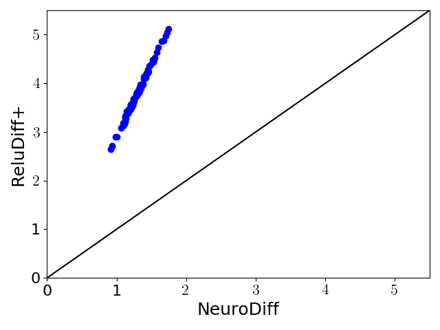
For MNIST, we focus on the 4x1024 network, which is the largest network considered by Paulsen et al. (Paulsen et al. 2020). In contrast, since the smaller networks, namely 3x100 and 2x512 networks, were handled easily by both tools, we omit their results. In the MNIST-related verification tasks, the goal is to verify for the given input region. We consider the two types of input regions from the previous work, namely global perturbations and targeted pixel perturbations, however we use input regions that are hundreds of orders of magnitude larger.
First, we look at the global perturbation. For these, the input space is created by taking an input image and then allowing a perturbation of +/- greyscale units to all of its pixels. In the previous work, the largest perturbation was . Figure 12 compares NeuroDiff and ReluDiff+ on all the way up to 8, where the x-axis is the perturbation applied, and the y-axis is the percentage of verification tasks (out of 100) that each can handle.
The results show that NeuroDiff can handle perturbations up to +/- 6 units, whereas ReluDiff+ begins to struggle at 4. While the difference between 4 and 6, may seem small, the volume of input space for a perturbation of 6 is times larger than 4, or in other words, 138 orders of magnitude larger.
Next, we show a comparison of the epsilon verified by a single forward pass for a perturbation of 8 on the MNIST 4x1024 network in Figure 12. Points above the blue line indicate NeuroDiff performed better. Overall, NeuroDiff is between two and three times more accurate than ReluDiff+.
Finally, we look at the targeted pixel perturbation properties. For these, the input space is created by taking an image, randomly choosing pixels, and setting there bounds to , i.e., allowing arbitrary changes to the chosen pixels. We again use the 4x1024 MNIST network. The results are summarized in Table 3. The first column shows the number of randomly perturbed pixels. We can again see very large speedups, and a significant increase in the size of the input region that NeuroDiff can handle.
| Num. Pixels | NeuroDiff (new) | ReluDiff+ | Speedup | ||||
| proved | undet. | time (s) | proved | undet. | time (s) | ||
| 15 | 100 | 0 | 236.5 | 100 | 0 | 1610.2 | 6.8 |
| 18 | 100 | 0 | 540.8 | 88 | 12 | 34505.8 | 63.8 |
| 21 | 100 | 0 | 1004.0 | 30 | 70 | 145064.5 | 144.5 |
| 24 | 99 | 1 | 7860.1 | 1 | 99 | 179715.9 | 22.9 |
| 27 | 83 | 17 | 49824.0 | 0 | 100 | 180000.0 | 3.6 |
5.3.4. Contribution of Each Technique
Here, we analyze the contribution of individual techniques, namely convex approximations and symbolic variables, to the overall performance improvement.
In Table 4, we present the average that was able to be verified after a single forward pass on the 4x1024 MNIST network for each of the four techniques: ReluDiff+ (baseline), NeuroDiff with only convex approximations, NeuroDiff with only intermediate variables, and the full NeuroDiff.
Overall, the individual benefits of the two proposed approximation techniques are obvious. While convex approximation (alone) consistently provides benefit as perturbation increases, the benefit of symbolic variables (alone) tends to decrease. In addition, combining the two provides much greater benefit than the sum of their individual contributions. With perturbation of 8, for example, convex approximations alone are 1.59 times more accurate than ReluDiff+, and intermediate variables alone are 1.01 times more accurate. However, together they are 2.93 times more accurate.
| Perturb | Average Verified | |||
| ReluDiff+ | Conv. Approx. | Int. Vars. | NeuroDiff | |
| 3 | 0.59 | 0.42 (+1.39x) | 0.43 (+1.38x) | 0.20 (+2.93x) |
| 4 | 1.02 | 0.70 (+1.46x) | 0.87 (+1.18x) | 0.36 (+2.85x) |
| 5 | 1.60 | 1.06 (+1.52x) | 1.47 (+1.09x) | 0.56 (+2.87x) |
| 6 | 2.29 | 1.47 (+1.55x) | 2.19 (+1.04x) | 0.79 (+2.90x) |
| 7 | 3.02 | 1.92 (+1.58x) | 2.96 (+1.02x) | 1.04 (+2.91x) |
| 8 | 3.80 | 2.39 (+1.59x) | 3.77 (+1.01x) | 1.30 (+2.93x) |
The results suggest two things. First, intermediate symbolic variables perform well when a significant portion of the network is already in the stable state. We confirm, by manually inspecting the experimental results, that it is indeed the case when we use a perturbation of 3 and 8 in the MNIST experiments. Second, the convex approximations provide the most benefit when the pre-ReLU delta intervals are (1) significantly wide, and (2) still contain a significant amount of symbolic information. This is also confirmed by manually inspecting our MNIST results: increasing the perturbation increases the overall width of the delta intervals.
6. Related Work
Aside from ReluDiff (Paulsen et al. 2020), the most closely related to our work are those that focus on verifying properties of single networks as opposed to two or more networks. These verification approaches can be broadly categorized into those that use exact, constraint solving-based techniques and those that use approximations.
On the constraint solving side, several works have adapted off-the-shelf solvers (Carlini and Wagner 2017; Tjeng et al. 2019; Bastani et al. 2016; Ehlers 2017; Baluta et al. 2019), or even implemented solvers specifically for neural networks (Katz et al. 2017; Katz et al. 2019). On the approximation side, many use techniques that fit into the framework of abstract interpretation (Cousot and Cousot 1977). For example, many works have leveraged abstract domains such as intervals (Wang et al. 2018c; Weng et al. 2018; Zhang et al. 2018; Julian et al. 2018), polyhedra (Singh et al. 2019a; Singh et al. 2019b), and zonotopes (Singh et al. 2019c; Gehr et al. 2018).
In addition, these verification techniques have also been combined (Singh et al. 2019c; Wang et al. 2018b; Huang et al. 2017), or entirely different approaches (Ruan et al. 2018; Dvijotham et al. 2018; Gopinath et al. 2018), such as bounding a network’s lipschitz constant, have been studied. These verification techniques can also be integrated into the training process to produce more robust and easier to verify networks (Fischer et al. 2019; Mirman et al. 2018; Wong and Kolter 2018; Mislav Balunovic 2020). These works are orthogonal, though we believe their techniques can be adapted to our domain.
A related but tangential line of work focuses on discovering interesting behaviors of neural networks, though without any guarantees. Most closely related to our work are differential testing techniques (Xie et al. 2019b; Pei et al. 2017; Ma et al. 2018b), which focus on finding disagreements between a set of networks. However, these techniques do not attempt to prove the equivalence or similarity of multiple networks.
Other works are more geared towards single network testing, and use white-box testing techniques (Ma et al. 2018a; Xie et al. 2019a; Sun et al. 2018; Tian et al. 2018; Odena and Goodfellow 2018), such as neuron coverage statistics, to assess how well a network has been tested, and also report interesting behaviors. Both of these can be thought of as adapting software engineering techniques to machine learning.
In addition, many works use machine learning techniques, such as gradient optimization, to find interesting behaviors, such as adversarial examples(Kurakin et al. 2017; Madry et al. 2018; Nguyen et al. 2015; Xu et al. 2016; Moosavi-Dezfooli et al. 2016). These interesting behaviors can then be used to retrain the network to improve robustness (Goodfellow et al. 2015; Raghunathan et al. 2018). Again, these techniques do not provide guarantees, though we believe they could be integrated into NeuroDiff to quickly find counterexamples.
Finally, our work draws inspiration from classic software engineering techniques, such as regression testing (Rothermel and Harrold 1997), differential assertion checking (Lahiri et al. 2013), differential fuzzing (Nilizadeh et al. 2019), and incremental symbolic execution (Person et al. 2011; Guo et al. 2016), where one version of a program is used as an “oracle”, to more efficiently test or verify a new version of the same program. In our case, can be thought of as the oracle, while is the new version.
7. Conclusions
We have presented NeuroDiff, a scalable differential verification technique for soundly bounding the difference between two feed-forward neural networks. NeuroDiff leverages novel convex approximations, which reduce the overall approximation error, and intermediate symbolic variables, which control the error explosion, to significantly improve efficiency and accuracy of the analysis. Our experimental evaluation shows that NeuroDiff can achieve up to 1000X speedup and is up to five times as accurate.
Acknowledgments
This work was partially funded by the U.S. Office of Naval Research (ONR) under the grant N00014-17-1-2896.
References
- (1)
- Anguita et al. (2013) Davide Anguita, Alessandro Ghio, Luca Oneto, Xavier Parra, and Jorge L. Reyes-Ortiz. 2013. A Public Domain Dataset for Human Activity Recognition Using Smartphones. 21st European Symposium on Artificial Neural Networks, Computational Intelligence and Machine Learning (2013).
- Baluta et al. (2019) Teodora Baluta, Shiqi Shen, Shweta Shinde, Kuldeep S Meel, and Prateek Saxena. 2019. Quantitative verification of neural networks and its security applications. In Proceedings of the 2019 ACM SIGSAC Conference on Computer and Communications Security. 1249–1264.
- Bastani et al. (2016) Osbert Bastani, Yani Ioannou, Leonidas Lampropoulos, Dimitrios Vytiniotis, Aditya V. Nori, and Antonio Criminisi. 2016. Measuring Neural Net Robustness with Constraints. In Annual Conference on Neural Information Processing Systems. 2613–2621.
- Carlini and Wagner (2017) Nicholas Carlini and David A. Wagner. 2017. Towards Evaluating the Robustness of Neural Networks. In IEEE Symposium on Security and Privacy. 39–57.
- Cousot and Cousot (1977) Patrick Cousot and Radhia Cousot. 1977. Abstract Interpretation: A Unified Lattice Model for Static Analysis of Programs by Construction or Approximation of Fixpoints. In ACM SIGACT-SIGPLAN Symposium on Principles of Programming Languages. 238–252.
- Dvijotham et al. (2018) Krishnamurthy Dvijotham, Robert Stanforth, Sven Gowal, Timothy A. Mann, and Pushmeet Kohli. 2018. A Dual Approach to Scalable Verification of Deep Networks. In International Conference on Uncertainty in Artificial Intelligence. 550–559.
- Ehlers (2017) Rüdiger Ehlers. 2017. Formal Verification of Piece-Wise Linear Feed-Forward Neural Networks. In Automated Technology for Verification and Analysis - 15th International Symposium, ATVA 2017, Pune, India, October 3-6, 2017, Proceedings. 269–286.
- Fischer et al. (2019) Marc Fischer, Mislav Balunovic, Dana Drachsler-Cohen, Timon Gehr, Ce Zhang, and Martin T. Vechev. 2019. DL2: Training and Querying Neural Networks with Logic. In International Conference on Machine Learning. 1931–1941.
- Gehr et al. (2018) Timon Gehr, Matthew Mirman, Dana Drachsler-Cohen, Petar Tsankov, Swarat Chaudhuri, and Martin T. Vechev. 2018. AI2: Safety and Robustness Certification of Neural Networks with Abstract Interpretation. In IEEE Symposium on Security and Privacy. 3–18.
- Gokulanathan et al. (2019) Sumathi Gokulanathan, Alexander Feldsher, Adi Malca, Clark Barrett, and Guy Katz. 2019. Simplifying Neural Networks with the Marabou Verification Engine. arXiv preprint arXiv:1910.12396 (2019).
- Goodfellow et al. (2015) Ian J. Goodfellow, Jonathon Shlens, and Christian Szegedy. 2015. Explaining and Harnessing Adversarial Examples. In International Conference on Learning Representations.
- Gopinath et al. (2018) Divya Gopinath, Guy Katz, Corina S. Pasareanu, and Clark W. Barrett. 2018. DeepSafe: A Data-Driven Approach for Assessing Robustness of Neural Networks. In Automated Technology for Verification and Analysis - 16th International Symposium, ATVA 2018, Los Angeles, CA, USA, October 7-10, 2018, Proceedings. 3–19.
- Guo et al. (2016) Shengjian Guo, Markus Kusano, and Chao Wang. 2016. Conc-iSE: Incremental Symbolic Execution of Concurrent Software. In IEEE/ACM International Conference On Automated Software Engineering.
- Han et al. (2016) Song Han, Huizi Mao, and William J. Dally. 2016. Deep Compression: Compressing Deep Neural Network with Pruning, Trained Quantization and Huffman Coding. In International Conference on Learning Representations.
- Huang et al. (2017) Xiaowei Huang, Marta Kwiatkowska, Sen Wang, and Min Wu. 2017. Safety Verification of Deep Neural Networks. In International Conference on Computer Aided Verification. 3–29.
- Julian et al. (2018) Kyle D. Julian, Mykel J. Kochenderfer, and Michael P. Owen. 2018. Deep Neural Network Compression for Aircraft Collision Avoidance Systems. CoRR abs/1810.04240 (2018). arXiv:1810.04240 http://arxiv.org/abs/1810.04240
- Katz et al. (2017) Guy Katz, Clark W. Barrett, David L. Dill, Kyle Julian, and Mykel J. Kochenderfer. 2017. Reluplex: An Efficient SMT Solver for Verifying Deep Neural Networks. In International Conference on Computer Aided Verification. 97–117.
- Katz et al. (2019) Guy Katz, Derek A. Huang, Duligur Ibeling, Kyle Julian, Christopher Lazarus, Rachel Lim, Parth Shah, Shantanu Thakoor, Haoze Wu, Aleksandar Zeljic, David L. Dill, Mykel J. Kochenderfer, and Clark W. Barrett. 2019. The Marabou Framework for Verification and Analysis of Deep Neural Networks. In International Conference on Computer Aided Verification. 443–452.
- Kurakin et al. (2017) Alexey Kurakin, Ian J. Goodfellow, and Samy Bengio. 2017. Adversarial examples in the physical world. In International Conference on Learning Representations.
- Lahiri et al. (2013) Shuvendu K Lahiri, Kenneth L McMillan, Rahul Sharma, and Chris Hawblitzel. 2013. Differential assertion checking. In Proceedings of the 2013 9th Joint Meeting on Foundations of Software Engineering. ACM, 345–355.
- Lecun et al. (1998) Yann Lecun, Leon Bottou, Yoshua Bengio, and Patrick Haffner. 1998. Gradient-based learning applied to document recognition. Proc. IEEE 86, 11 (1998), 2278–2324.
- Ma et al. (2018a) Lei Ma, Felix Juefei-Xu, Fuyuan Zhang, Jiyuan Sun, Minhui Xue, Bo Li, Chunyang Chen, Ting Su, Li Li, Yang Liu, et al. 2018a. Deepgauge: Multi-granularity testing criteria for deep learning systems. In IEEE/ACM International Conference On Automated Software Engineering. ACM, 120–131.
- Ma et al. (2018b) Shiqing Ma, Yingqi Liu, Wen-Chuan Lee, Xiangyu Zhang, and Ananth Grama. 2018b. MODE: automated neural network model debugging via state differential analysis and input selection. In Proceedings of the 2018 ACM Joint Meeting on European Software Engineering Conference and Symposium on the Foundations of Software Engineering, ESEC/SIGSOFT FSE 2018, Lake Buena Vista, FL, USA, November 04-09, 2018. 175–186.
- Madry et al. (2018) Aleksander Madry, Aleksandar Makelov, Ludwig Schmidt, Dimitris Tsipras, and Adrian Vladu. 2018. Towards deep learning models resistant to adversarial attacks. International Conference on Learning Representations (2018).
- Mirman et al. (2018) Matthew Mirman, Timon Gehr, and Martin T. Vechev. 2018. Differentiable Abstract Interpretation for Provably Robust Neural Networks. In International Conference on Machine Learning. 3575–3583.
- Mislav Balunovic (2020) Martin Vechev Mislav Balunovic. 2020. Adversarial Training and Provable Defenses: Bridging the Gap. International Conference on Learning Representations.
- Moore et al. (2009) Ramon E Moore, R Baker Kearfott, and Michael J Cloud. 2009. Introduction to interval analysis. Vol. 110. Siam.
- Moosavi-Dezfooli et al. (2016) Seyed-Mohsen Moosavi-Dezfooli, Alhussein Fawzi, and Pascal Frossard. 2016. DeepFool: A Simple and Accurate Method to Fool Deep Neural Networks. In IEEE Conference on Computer Vision and Pattern Recognition. 2574–2582.
- Nguyen et al. (2015) Anh Mai Nguyen, Jason Yosinski, and Jeff Clune. 2015. Deep neural networks are easily fooled: High confidence predictions for unrecognizable images. In IEEE Conference on Computer Vision and Pattern Recognition. 427–436.
- Nilizadeh et al. (2019) Shirin Nilizadeh, Yannic Noller, and Corina S. Pasareanu. 2019. DifFuzz: differential fuzzing for side-channel analysis. In International Conference on Software Engineering. 176–187.
- Odena and Goodfellow (2018) Augustus Odena and Ian Goodfellow. 2018. Tensorfuzz: Debugging neural networks with coverage-guided fuzzing. arXiv preprint arXiv:1807.10875 (2018).
- Paulsen (2020) Brandon Paulsen. 2020. ReluDiff-ICSE2020-Artifact. https://github.com/pauls658/ReluDiff-ICSE2020-Artifact.
- Paulsen et al. (2020) Brandon Paulsen, Jingbo Wang, and Chao Wang. 2020. ReluDiff: Differential Verification of Deep Neural Networks. International Conference on Software Engineering (2020).
- Pei et al. (2017) Kexin Pei, Yinzhi Cao, Junfeng Yang, and Suman Jana. 2017. DeepXplore: Automated Whitebox Testing of Deep Learning Systems. In ACM symposium on Operating Systems Principles. 1–18.
- Person et al. (2011) Suzette Person, Guowei Yang, Neha Rungta, and Sarfraz Khurshid. 2011. Directed Incremental Symbolic Execution. In ACM SIGPLAN Conference on Programming Language Design and Implementation. ACM, New York, NY, USA, 504–515.
- Raghunathan et al. (2018) Aditi Raghunathan, Jacob Steinhardt, and Percy Liang. 2018. Certified Defenses against Adversarial Examples. In International Conference on Learning Representations.
- Rothermel and Harrold (1997) Gregg Rothermel and Mary Jean Harrold. 1997. A safe, efficient regression test selection technique. ACM Transactions on Software Engineering and Methodology (TOSEM) 6, 2 (1997), 173–210.
- Ruan et al. (2018) Wenjie Ruan, Xiaowei Huang, and Marta Kwiatkowska. 2018. Reachability Analysis of Deep Neural Networks with Provable Guarantees. In International Joint Conference on Artificial Intelligence. 2651–2659.
- Singh et al. (2019a) Gagandeep Singh, Rupanshu Ganvir, Markus Püschel, and Martin Vechev. 2019a. Beyond the Single Neuron Convex Barrier for Neural Network Certification. In Advances in Neural Information Processing Systems (NeurIPS).
- Singh et al. (2019b) Gagandeep Singh, Timon Gehr, Markus Püschel, and Martin T. Vechev. 2019b. An abstract domain for certifying neural networks. ACM SIGACT-SIGPLAN Symposium on Principles of Programming Languages (2019), 41:1–41:30.
- Singh et al. (2019c) Gagandeep Singh, Timon Gehr, Markus Püschel, and Martin T. Vechev. 2019c. Boosting Robustness Certification of Neural Networks. In International Conference on Learning Representations.
- Sun et al. (2018) Youcheng Sun, Min Wu, Wenjie Ruan, Xiaowei Huang, Marta Kwiatkowska, and Daniel Kroening. 2018. Concolic testing for deep neural networks. In Proceedings of the 33rd ACM/IEEE International Conference on Automated Software Engineering, ASE 2018, Montpellier, France, September 3-7, 2018. 109–119.
- Szegedy et al. (2013) Christian Szegedy, Wojciech Zaremba, Ilya Sutskever, Joan Bruna, Dumitru Erhan, Ian Goodfellow, and Rob Fergus. 2013. Intriguing properties of neural networks. arXiv preprint arXiv:1312.6199 (2013).
- Tian et al. (2018) Yuchi Tian, Kexin Pei, Suman Jana, and Baishakhi Ray. 2018. DeepTest: Automated testing of deep-neural-network-driven autonomous cars. In International Conference on Software Engineering. 303–314.
- Tjeng et al. (2019) Vincent Tjeng, Kai Xiao, and Russ Tedrake. 2019. Evaluating robustness of neural networks with mixed integer programming. International Conference on Learning Representations (2019).
- Wang et al. (2018a) Liwei Wang, Lunjia Hu, Jiayuan Gu, Zhiqiang Hu, Yue Wu, Kun He, and John Hopcroft. 2018a. Towards understanding learning representations: To what extent do different neural networks learn the same representation. In Advances in Neural Information Processing Systems. 9584–9593.
- Wang et al. (2018b) Shiqi Wang, Kexin Pei, Justin Whitehouse, Junfeng Yang, and Suman Jana. 2018b. Efficient Formal Safety Analysis of Neural Networks. In Annual Conference on Neural Information Processing Systems. 6369–6379.
- Wang et al. (2018c) Shiqi Wang, Kexin Pei, Justin Whitehouse, Junfeng Yang, and Suman Jana. 2018c. Formal Security Analysis of Neural Networks using Symbolic Intervals. In USENIX Security Symposium. 1599–1614.
- Weng et al. (2018) Tsui-Wei Weng, Huan Zhang, Hongge Chen, Zhao Song, Cho-Jui Hsieh, Luca Daniel, Duane S. Boning, and Inderjit S. Dhillon. 2018. Towards Fast Computation of Certified Robustness for ReLU Networks. In International Conference on Machine Learning. 5273–5282.
- Wong and Kolter (2018) Eric Wong and J. Zico Kolter. 2018. Provable Defenses against Adversarial Examples via the Convex Outer Adversarial Polytope. In International Conference on Machine Learning. 5283–5292.
- Xie et al. (2019a) Xiaofei Xie, Lei Ma, Felix Juefei-Xu, Minhui Xue, Hongxu Chen, Yang Liu, Jianjun Zhao, Bo Li, Jianxiong Yin, and Simon See. 2019a. DeepHunter: a coverage-guided fuzz testing framework for deep neural networks. In Proceedings of the 28th ACM SIGSOFT International Symposium on Software Testing and Analysis. 146–157.
- Xie et al. (2019b) Xiaofei Xie, Lei Ma, Haijun Wang, Yuekang Li, Yang Liu, and Xiaohong Li. 2019b. Diffchaser: Detecting disagreements for deep neural networks. In Proceedings of the 28th International Joint Conference on Artificial Intelligence. AAAI Press, 5772–5778.
- Xu et al. (2016) Weilin Xu, Yanjun Qi, and David Evans. 2016. Automatically Evading Classifiers: A Case Study on PDF Malware Classifiers. In Network and Distributed System Security Symposium.
- Zhang et al. (2018) Huan Zhang, Tsui-Wei Weng, Pin-Yu Chen, Cho-Jui Hsieh, and Luca Daniel. 2018. Efficient neural network robustness certification with general activation functions. In Advances in neural information processing systems. 4939–4948.
- Zhang et al. (2012) Xianyi Zhang, Qian Wang, and Yunquan Zhang. 2012. Model-driven Level 3 BLAS Performance Optimization on Loongson 3A Processor. In 18th IEEE International Conference on Parallel and Distributed Systems, ICPADS 2012, Singapore, December 17-19, 2012. 684–691.