Deep Autoencoders:
From Understanding to Generalization Guarantees

An Autoencoder (AE) aims at learning an identity mapping, also known as auto-association Ackley et al. 1985, on a given dataset with a bottleneck latent dimension. It has been implemented first for image compression Cottrell et al. 1987, speech recognition Elman and Zipser 1988, and dimensionality reduction Baldi and Hornik 1989. It is composed of two nonlinear maps: an encoder, denoted by $\boldsymbol{E}$ and a decoder, denoted by $\boldsymbol{D}$. The encoder maps an input $x\in\mathbb{R}^{d}$ to a hidden layer of dimension $h<d$, $\boldsymbol{E}(\boldsymbol{x})$, which encodes the salient features in the data Goodfellow et al. 2016 and defines its code or embedding. The decoder reconstructs the input from its code, thus the entire AE map is defined as $\left(\boldsymbol{D}\circ\boldsymbol{E}\right)(\boldsymbol{x})$ with $\circ$ denoting the composition operator.

The weights of the AE are learned based on some flavors of reconstruction losses, e.g., the mean-square error for real data and the binary cross-entropy for binary data, between the output, $\left(\boldsymbol{D}\circ\boldsymbol{E}\right)(\boldsymbol{x})$, and the input, $\boldsymbol{x}$. To improve generalization, some regularizations can complement the reconstruction loss Srivastava et al. 2014 such as favoring sparsity of the code Makhzani and Frey 2013 or sparsity of the weights Jarrett et al.. Other types of regularization include injecting noise in the input leading to Denoising AE known to increase the robustness to small input perturbations Vincent et al. 2008. Closer to our work, Rifai et al. 2011a and Rifai et al. 2011b proposed to improve the robustness of the code to small input perturbations by penalizing the curvature of the encoder mapping by regularizing the Jacobian as well as the Hessian of $\boldsymbol{E}$.

A DN is an operator $\boldsymbol{f}_{\Theta}$ with parameters $\Theta$ composing $L$ intermediate layer mappings $\boldsymbol{f}_{\ell}$, $\ell=1,\dots,L$, that combine affine and simple nonlinear operators such as the fully connected operator, convolution operator, activation operator (applying a scalar nonlinearity such as the ubiquitous ReLU), or pooling operator.

A DN employing nonlinearities such as (leaky-)ReLU, absolute value, and max-pooling is a continuous piecewise linear operator and thus lives on a partition $\Omega$ of the input space. As such, the DN’s CPA mapping of an input $\boldsymbol{x}$ can be written as

where $1$ defines the indicator function, $A_{\omega}$ and $B_{\omega}$ the per region affine parameters involving the DN per layer affine parameters , $W^{\ell},\boldsymbol{b}^{\ell}\in\Theta,\forall\ell$, and the nonlinearities state of the region $\omega\in\Omega$ (Balestriero and Baraniuk 2018a). The unit and layer input space partitioning can be rewritten as Power Diagrams, a generalization of Voronoi Diagrams (Balestriero et al. 2019); composing layers produce a Power Diagram subdivision.

The approaches mentioned in the introduction aiming at enhancing the capability of DNs to take into account the symmetries in the data consider only those that are explicitly modeled, s.a., translation, another line of work consists in learning them from the data. In Rao and Ruderman 1999; Sohl-Dickstein et al. 2010; Hashimoto et al. 2017; Bahroun et al. 2019; Cosentino and Aazhang 2020, they propose methods capable of discovering the symmetry within the data alleviating the need for explicitly defining appropriate equivalence classes for the data. In fact, in a simple computer vision dataset such as MNIST or in a music retrieval dataset such as GTZAN, there is more than translation and rotation to characterize efficiently the data (Ick and Lostanlen 2020). This paragraph is dedicated to the understanding of such approximation methods, which will be an important part of our regularizations.

The approximation of Lie groups has been introduced by Rao and Ruderman 1999 and later extended in Sohl-Dickstein et al. 2010; Wang et al. 2011, and aims at learning the transformation operator underlying the data with the assumption that the dataset is the result of the action of a group on a sample. This framework has an essential place in neuroscience as there is evidence of an underlying network of neurons enabling the detection of a class of equivalence via transformation learning (Kriegeskorte et al. 2008; Sengupta et al. 2018; Bahroun et al. 2019).

In the case of a Lie group, the dataset can be modeled according to the first-order Lie equation

where $\boldsymbol{x}(\theta)\in\mathbb{R}^{d}$, $\theta$ is the coefficient governing the amount of transformation, and $G\in\mathbb{R}^{d\times d}$. This first-order differential equation indicates that the variation of the data is linear with respect to the data and depends on the infinitesimal operator $G\in\mathcal{T}_{I}\mathcal{G}$ where $\mathcal{T}_{I}\mathcal{G}$ denotes the Lie algebra of the group $\mathcal{G}$, i.e., the tangent of the group at the identity element. An introduction to group transformations can be found in Hall 2015. The solution of Eq. 2 is given by $\boldsymbol{x}(\theta)=\exp(\theta G)\boldsymbol{x}(0)$, a simple example with the group of rotation is given in Appendix C.

While the learnability of the exponential map is tedious, one can exploit its Taylor series expansion to learn the infinitesimal operator. In fact, for a small $\epsilon$ we have

The operator $G$ can thus be learned using data that are close to each other as they result from small transformations and thus follow this approximation. Without this form of supervision, the search for neighbor data is achieved by the nearest neighbor algorithm, as in Hashimoto et al. 2017. Note that in our case, we will consider multiple transformations, each parametrized by a $1$-dimensional Lie group, i.e. $\textbf{x}(\theta)=\prod_{k=1}^{h}\exp(\theta_k G_k)\textbf{x}(0)$, where $\theta\in\mathbb{R}^{h}$. In that case the first order approximation around the identity element of each group, as Eq. 3, becomes $\boldsymbol{x}(\theta+\epsilon)\approx(I+\sum_{k=1}^{h}\epsilon_{k}G_{k})\boldsymbol{x}(\theta)$, where $\epsilon\in\mathbb{R}^{h}$ and with $\epsilon_{k}$ being the transformation parameter associated to infinitesimal operator $G_{k}$.

Now, let $\omega\in\Omega^{E,D}$ defines a region induced by the AE partitioning in the input space as described in Sec. 2.2. Given a d-dimensional sample $\boldsymbol{x}\in\omega$, the max affine spline formulation of the AE mapping is defined as

where $\circ$ is the composition operator, $A^{D}_{\omega}\in\mathbb{R}^{d\times h},A^{E}_{\omega}\in\mathbb{R}^{h\times d},B^{E}_{\omega}\in\mathbb{R}^{h}$ and $B^{D}_{\omega}\in\mathbb{R}^{d}$ with $d$ being the dimension of the input space and $h$ the bottleneck dimension.

The mapping from these global parameters to the per-layer ones is performed as follows. First, we denote by $W^{\ell}\in\mathbb{R}^{d_{\ell}\times d_{\ell-1}},\boldsymbol{b}^{\ell}\in\mathbb{R}^{d_{\ell}}$ the affine parameters of each layer, where $\ell\in\left\{1,\dots,L\right\}$ defines the encoder indexes and $\ell\in\left\{L+1,\dots,L+P\right\}$ the decoder ones (with structure depending on the layer type), where $L$ denotes the number of encoder layers, $P$ the number of decoder layers, $d_{\ell-1}$ the input dimension of the layer $\ell$ and $d_{\ell}$ its output dimension. We have that $d_{L}=h$ the bottleneck dimension, $d_{0}=d_{L+P}=d$ the input and output dimension. Then, we also denote by $Q^{\ell}$ the diagonal matrices encoding the region induced states of the nonlinearities, $(0,1)$ for ReLU, $(-1,1)$ for absolute value. Finally, the parameters of the max affine spline AE formulation described in Eq. 4 are defined as

$A^{D}_{\omega}$ and $A^{D}_{\omega}$ are defined similarly with $\ell\in\left\{L+1,\dots,L+P\right\}$. Therefore, there is a direct mapping from the intuitive piecewise affine parameterization of the network to the per-layer parametrization as it is commonly used in the literature.

Given these analytical maps, we now provide insights into the AE approximation. Let’s rewrite Eq. 4 as

where $B^{E,D}_{\omega}=A^{D}_{\omega}B^{E}_{\omega}+B^{D}_{\omega}$, $\textbf{a}^{E^{T}}_{k}[\omega]$ are the rows of $A^{E}_{\omega}$, $\textbf{a}^{D}_{k}[\omega]$ are the columns of $A^{D}_{\omega}$. This is the shifted mapping of $\boldsymbol{x}$ onto the subspace spanned by $A^{D}_{\omega}$ and with coordinates driven by $A^{E}_{\omega}$.

From Eq. 6, we deduce the per region role of the encoder and decoder. The samples of each region $\omega\in\Omega^{E,D}$, are expressed in the basis defined by the decoder region-dependent parameter $A^{D}_{\omega}$, i.e., the per region parametric representation of the approximated manifold, and the coordinates of this sample in such a basis are induced by the region-dependent parameter $A^{E}_{\omega}$, the whole mapping is then shifted according to both the encoder and decoder CPA parameters.

We now derive a necessary condition on the CPA parameters, $A^{D}_{\omega},A^{E}_{\omega}$, such that the AE achieves perfect reconstruction on a given continuous piecewise linear surface in the case of zero bias as often used in practice Mohan et al. 2020.

That is, if a continuous piecewise linear surface is correctly approximated, we know that the parameters of the MAS operator describing the encoder and decoder will be bi-orthogonal, i.e., the column vectors of $A^{D}_{\omega}$ and the row vectors of $A^{E}_{\omega}$ form a bi-orthogonal basis.

We now propose to give intuitions regarding this condition by utilizing the mapping between CPA parameters and layer weights as per Eq. 5. In fact, the following corollary provides the conditions for the bi-orthogonality to be fulfilled depending on the weights of the autoencoder, i.e., $W^{\ell}$. For the sake of clarity, we consider the case of a $2$-layer ReLU AE.

This results shows that the bi-orthogonality condition can be obtained via a combination of orthogonality conditions between the weights and/or nonlinearity activations.

For instance, the proposition $(i)$ corresponds to the case where the input of the $k^{\prime}$ unit in the bottleneck layer is negative, condition $(ii)$ is the case where the input of all output units is negative, condition $(iii)$ corresponds to a linear decoder and orthogonality of the weights, and $(iv)$ corresponds to an orthogonality condition between the $k^{th}$ column of the decoder weight with the $k^{\prime th}$ row of the encoder weight modulo the activations of the decoder layer. Note that if $(ii)$ and $(iii)$ hold for multiple regions $\omega\in\Omega^{E,D}$ it implies that the decoder is linear with respect to the coordinate space and forms a linear manifold. Thus, these are not realistic conditions to have efficient AEs.

From the CPA formulation, we observed that for each region $\omega\in\Omega^{E,D}$, $\boldsymbol{D}\circ\boldsymbol{E}$ defines a composition of two continuous piecewise affine functions, each defined respectively by the parameters $A^{E}_{\omega}$, $B^{E}_{\omega}$, and $A^{D}_{\omega}$, $B^{D}_{\omega}$. We can thus derive simple analytical formulas for the per region Jacobian and approximated Hessian of the AE.

The Jacobian of the AE for a given region $\omega\in\Omega^{E,D}$ is given by

More details regarding the Jacobian are given in Appendix A.7. It is also clear that the rank of the Jacobian is upper bounded by the latent dimension as $\text{rank}(J_{\omega}[\boldsymbol{D}\circ\boldsymbol{E}])\leq h$, where $h$ is the number of units of the bottleneck layer of the AE, and in general by the $\min_{\ell}d_{\ell}$. This dimension is directly related to the manifold’s dimension that one aims to approximate, assuming that all other layer widths are larger than $h$.

One can similarly obtain the per region tangent of the decoder, as it defines the per region parametric representation of the manifold, see Fig. 2. We recall that we denote by $\Omega^{D}$ the partition of the latent space induced by the decoder

where the columns of $A^{D}_{\omega}$ form the basis of the tangent space induced by $\boldsymbol{D}$.

The characterization of the curvature of the approximation of the data manifold can be done using the per region Hessian defined by $H_{\omega},\forall\omega\in\Omega^{D}$, which in our case will be defined as the sum of the difference of neighboring tangent planes.

where $\mathcal{N}(\omega)$ denotes the set of neighbors of region $\omega$ and $\left\|.\right\|_{F}$ is the Frobenius norm. This approach is based on the derivation described in Rifai et al. 2011a. In practice, we use a stochastic approximation of the sum by generating a small mini-batch of a few corrupted samples which induce neighboring regions.

We are now interested in leveraging these findings to analyze and interpret common AE regularizations.

1. (i)

   Higher-Order Contractive AE (Rifai et al. 2011a): This regularization penalizes the energy of the first and approximated second derivative the encoder map for any region containing a training sample, i.e., $\left\|A^{E}_{\omega}\right\|_{F}$ and $\sum_{\omega^{\prime}\in\mathcal{N}(\omega)}\left\|A^{E}_{\omega}-A^{E}_{\omega^{\prime}}\right\|_{F}$. In the case of a ReLU AE, we know from Eq. 4 and the submultiplicativity of the Frobenius norm that the norm of the Jacobian is upper-bounded by $\left\|W^{L}\right\|_{F}\times\dots\times\left\|W^{1}\right\|_{F}$. Therefore adding a weight-decay penalty on the encoder weights induces the first-order contractive AE. The second-order induces the curvature of the piecewise linear map $A^{E}$ to be small. Note that it is the per-region affine map induced by the encoder that is regularized, and that it depends on the region’s activation codes, i.e., $Q^{i}$ and $W^{i}\;\;\forall i\in\left\{1,\dots,L\right\}$. Thus, if two neighboring regions have only have few changes in their code, and that the associated weights are small, then, such a constraint does not affect the overall curvature. On the other hand, if between two regions, the code of a unit having a weight with large amplitude does not change, then the regularization does not affect the curvature either, see details with a toy example in Appendix A.8.

2. (ii)

   Denoising AE (Vincent et al. 2008): Denoising AE is known to have a similar effect than the weight-decay penalty on the DN architecture Wager et al. 2013. A penalty on the energy of $W^{\ell}$ induces a penalty on the energy of the $A^{E}_{\omega}$ and $A^{D}_{\omega}$ $,\forall\omega\in\Omega^{E,D}$. Therefore, it constrains each piece’s slope to be as flat a possible, implying that the piecewise linear map focuses on approximating the low-frequency content in the data, which reinforces the learning bias of deep networks towards low-frequency information (Rahaman et al. 2018). Thus, we see how denoising and Higher-Order Contractive are tied together.

First, we want to understand under which condition a interpolation function $\boldsymbol{f}\in C^{2}(\mathbb{R},\mathbb{R}^{d})$ coincides with the orbit of $\boldsymbol{x}(0)\in\mathbb{R}^{d}\setminus\left\{0\right\}$ under the action of the group $\mathcal{G}$. In particular, we propose to exploit a regularization that induces an orbit of a Lie group, such as

where $\frac{d^{k}\boldsymbol{f}(\theta)}{d\theta^{k}}$ denotes the $k^{th}$ order derivative of $\boldsymbol{f}$.

This regularization constrains $\boldsymbol{f}$ such that its $k^{th}$ order derivative is a linear map of the $k-1$ order. In the following theorem, we show that, for $k\in\left\{1,2\right\}$, such regularization coupled with an interpolation loss function leads to a perfect approximation of the data manifold $x$. That is, $\boldsymbol{f}$ coincides with $\boldsymbol{x}(\theta)=\exp(\theta G)\boldsymbol{x}(0),\forall\theta\in\mathbb{R}$ if and only if $\frac{d^{k}\boldsymbol{f}(\theta)}{d\theta^{k}}=G\frac{d^{k-1}\boldsymbol{f}(\theta)}{d\theta^{k-1}}$ and it exists a certain number of $\theta_{i}$, depending on the order $k$, such that $\boldsymbol{f}(\theta_{i})=\boldsymbol{x}(\theta_{i})$. Note that the restriction to the first two orders is natural as we will apply these results on continuous piecewise affine maps, in which the second-order can only be approximated using stochastic approximation as per Sec. 3.3.

Thus an interpolant $\boldsymbol{f}$, can approximate the orbit of a Lie group, utilizing two components, the aforementioned regularization with $k\in\left\{1,2\right\}$, and a reconstruction error that force the interpolation function to coincide with $k$ training samples.

The derived regularizations were based on a smooth interpolant $\boldsymbol{f}$ and need to be adapted to the case of a CPA map. To do so, there are several crucial considerations:

1. (i)

   For the sake of clarity, the previous section illustrated the case of a one-dimensional group. Here we propose to generalize such an approach to multiple groups of transformations. We, therefore, consider the case of $h$ infinitesimal operators $G_{1},\dots,G_{h}$ each corresponding to a $1$-dimensional group, as explained in Sec. 2.3.

2. (ii)

   The second-order regularization requires constrains the Hessian of the CPA, which by definition, can only be approximated stochastically as explained in Sec. 3.3.

3. (iii)

   The assumption on the data is that they are generated by $h$ transformation groups. Thus, the intrinsic dimensionality of the data is at most $h$. Therefore, the size of the bottleneck layer, which corresponds to the maximum dimension of the manifold the autoencoder can generate (as per Sec. 3.1), is also $h$.

In Sec. 4.1, we showed that if the regularization defined in Eq. 10 is equal to zero for any given $k\in\left\{1,2\right\}$, and if the interpolation function $\boldsymbol{f}$ coincides with the data manifold defined by $\boldsymbol{x}$ on $k$ points, then $\boldsymbol{f}$ coincides with $\boldsymbol{x}$. We now derive the generalization guarantees in the particular case where $\boldsymbol{f}$ is a CPA approximant.

Based on the assumption that $(i)$ a region of the real manifold is correctly approximated, $(ii)$ one of the regularizations defined in Eq. 12,13 is minimized, and that $(iii)$ the infinitesimal operator $G$ obtained from the regularization coincides with the infinitesimal operator of the group governing the data, we obtain the following bound on the approximation of the data manifold.

The previous statement shows that if the number of pieces of the piecewise affine map, which depends on the number of neurons in the DN architecture (see Fig. 3 and refer to Montufar et al. 2014 for more details) and the type of nonlinearity, goes to infinity, then the decoder would coincide with the data manifold. In a practical setting, it tells us that the higher the number of regions is, the higher is the degrees of freedom of the CPA, and that under this regularization, these degrees of freedom are controlled while not requiring more training points.

The degrees of freedom of our regularized AE comprise the usual AE parameters (per layer affine transformations) and the parameters of each regularization. The $\epsilon$ values are found from the analytical form given by Propositions 2 and 3 in Appendix B. We learn the matrices $G_{k},\forall k\in\left\{1,\dots,h\right\}$ with gradient descent based optimizer (Kingma and Ba 2014) and thus our method introduces $hd^{2}$ additional parameters, where $d$ is the dimension of the input data. Note that a priori knowledge on the structure of the $G_{k}$ such as low-rank or skew-symmetric, i.e., Lie algebra of the special orthogonal group, can be imposed to reduce the number of parameters; we do not explore this in our study while it could be considered to speed up the computations and improve the regularization tractability. The regularizations themselves depend on the AE to find the optimal $\epsilon$ and adapt the matrices $G_{k}$. The dimension of each $G_{k}$ is quadratic in the dimension of the data. As such, for a high-dimensional datasets, the number of learnable parameters is large. Hence the optimization of the $G_{k}$ matrices remains the current bottleneck of the method. We propose to apply the regularization term during training starting from the random initialization. More advanced strategies such as scheduled alternating minimization or employing a warm-up phase could be leveraged and result in further improvement in performance.

We now describe how we approximate the regularization terms by removing the need to evaluate the entire input space partition of the decoder for the second-order term and removing the need to sample the entire domain for the first-order term.

Recall that in the proposed second-order regularization, one should have the knowledge of the decoder latent space partition. In practice, and for large networks, the discovery of the partition would not be feasible. We thus propose to approximate the regularization by only sampling some of the regions and some of their respective neighbors. This sampling is done by first randomly sampling some vectors in the AE latent space. As for each sample, the associated per region map is automatically formed during the foward pass of the decoder, the per region parameters can be obtained by computing the affine mapping induced by the samples. To compute the neighbors of those sample regions, we use a simple dichotomic search. That is, for each of the sampled regions, we sample another (nearby) vector and keep pushing this new sample toward the first sample until one obtains the closest sample that remains in a different region. With the above, one now has the knowledge of some regions and one neighboring region for each of those regions. We leverage this approach and perform the search of a single neighbor; for a better approximation of the regularization, one can repeat this sampling process and accumulate the obtained regions and neighbors. For the first-order term, we propose a similar approximation where we approximate the integral by sampling a latent space vector $\theta$ (at each mini-batch).

Let us now consider the computational complexity induced by the regularizations omitting the computational cost of a pass through the AE as it is shared across all techniques. The optimal coordinates $\epsilon^{*}$ are obtained by solving a linear system of $h$ equations in both cases for each sampled datum (first-order) or each sampled region (second-order). This equation has to be solved for each sample region or latent space vector; we denote this by $N$ as in our case, we sample in each mini-batch as many vectors/regions as the size of the mini-batch. We obtain the time complexity $\mathcal{O}(h^{2}N+d^{2}hN)$ for the first-order, and $\mathcal{O}(h^{2}N+d^{2}h^{2}N)$ for the second-order, and a space complexity of $\mathcal{O}(d^{2}h)$ in both cases being driven by the need to retain the matrices $G_{1},\dots,G_{h}$. The current bottleneck is the storage of those matrices, which limits the size of the AE bottleneck and output dimension.

We evaluate our framework on diverse datasets, including images and time-series data including speech, medical as well a seismic recordings, the description of the datasets is given in Appendix D. For each model and each hyperparameter, we perform $10$ runs for $125$ epochs with batch size $16$. The results are reported in Table 1. In this table, the statistics reported correspond to the average over the $10$ runs, each run using the test set performances based on the best validation set measure. Note that for CIFAR$10$, the computational burden of both the second-order Lie group regularization and the higher-order contractive one is too high. Thus only the AE, denoising AE and the first-order Lie group regularization are evaluated.

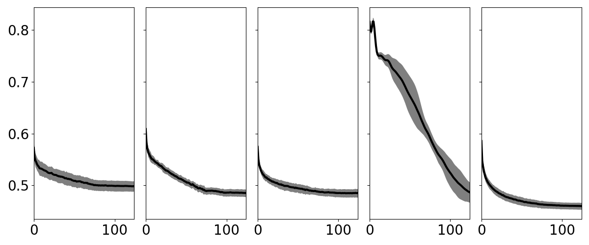
We propose, in particular, to visualize the test set reconstruction for the different AE models during training in Fig. 4 (see Fig. 6 in Appendix E for supplementary figures), where we can see that both Lie Group AEs are robust to the DN initialization and do not overfit. Besides, we can observe that while the first order on this dataset outperforms all the other regularizations, its variance at the begining of the learning phase is more volatile than other approaches.

The hyperparameter responsible for the variance of the noise added to the data in the Denoising AE case also corresponding to the noise added to the data to sample Jacobian of nearby regions in Higher-Order Contractive AE parameter is evaluated for the values $\left\{0.001,0.01,0.1,1\right\}$. Another hyperparameter is the regularization trade-off parameter for both the Higher-Order Contractive AE and Lie Group AEs, the following values are tested for both models $\left\{0.001,0.01,0.1,1,10,100,1000\right\}$. All the models were trained using the same AE with $3$ fully connected encoder layers with ReLU with bottleneck dimension $h=10$, and $3$ fully connected decoder layer with ReLU and $1$ linear fully connected output layer.

We can observe in Table 1 that the Lie group regularizations are usually outperforming the other methods the different datasets we evaluated. While the second-order regularization is more computationally demanding, it appears to be more stable and robust to the change of parameters. Besides, we can see that the first-order regularization might be more sensitive to how close to a Lie group the dataset under evaluation is. In fact, both the first and second-order depends on the learned infinitesimal operator, however, while the second-order use such matrix to constrain the overall curvature of the CPA the first-order use it to constrains its mapping.

In Fig. 5, we show, for three datasets, the value of the parameters $\epsilon_{i},\forall i\in\left\{1,\dots,h\right\}$ obtained by minimizing Eq. 12. This observation is important as the framework we propose assumes that the dimension of the orbit, hence the number of group transformations, is the same as the dimension of the bottleneck layer of the autoencoder. In particular, we propose to highlight the sparsity of the parameters, i.e., if for various sampled pairs, the value a particular strength parameter, $\epsilon_{i}$, is close to $0$. If it is, then the associated group of transformation is not being used to map any $\textbf{D}(\theta)$ to a close sample $\textbf{D}(\theta^{\prime})$. Therefore, the number of group of transformations selected is too large, e.g., in the top right subplot, corresponding to the Haptics dataset, we observe that, the $10$ transformations are not required.

References

- Ackley et al. (1985) D. H. Ackley, G. E. Hinton, and T. J. Sejnowski. A learning algorithm for boltzmann machines. Cognitive science, 9(1):147–169, 1985.
- Andén and Mallat (2014) J. Andén and S. Mallat. Deep scattering spectrum. IEEE Transactions on Signal Processing, 62(16):4114–4128, 2014.
- Andén et al. (2015) J. Andén, V. Lostanlen, and S. Mallat. Joint time-frequency scattering for audio classification. CoRR, abs/1512.02125, 2015.
- Bagnall et al. (2017) A. Bagnall, J. Lines, A. Bostrom, J. Large, and E. Keogh. The great time series classification bake off: a review and experimental evaluation of recent algorithmic advances. Data Mining and Knowledge Discovery, 31:606–660, 2017.
- Bahroun et al. (2019) Y. Bahroun, D. Chklovskii, and A. Sengupta. A similarity-preserving network trained on transformed images recapitulates salient features of the fly motion detection circuit. In Advances in Neural Information Processing Systems, pages 14178–14189, 2019.
- Baldi and Hornik (1989) P. Baldi and K. Hornik. Neural networks and principal component analysis: Learning from examples without local minima. Neural networks, 2(1):53–58, 1989.
- Balestriero and Baraniuk (2018a) R. Balestriero and R. Baraniuk. A spline theory of deep learning. In International Conference on Machine Learning, pages 374–383, 2018a.
- Balestriero and Baraniuk (2018b) R. Balestriero and R. G. Baraniuk. Mad max: Affine spline insights into deep learning. arXiv preprint arXiv:1805.06576, 2018b.
- Balestriero et al. (2019) R. Balestriero, R. Cosentino, B. Aazhang, and R. Baraniuk. The geometry of deep networks: power diagram subdivision. In Advances in Neural Information Processing Systems, pages 15806–15815, 2019.
- Bruna and Mallat (2013) J. Bruna and S. Mallat. Invariant scattering convolution networks. IEEE transactions on pattern analysis and machine intelligence, 35(8):1872–1886, 2013.
- Chen et al. (2014) X. Chen, X. Cheng, and S. Mallat. Unsupervised deep haar scattering on graphs. In Advances in Neural Information Processing Systems, pages 1709–1717, 2014.
- Cheng et al. (2018) Z. Cheng, H. Sun, M. Takeuchi, and J. Katto. Deep convolutional autoencoder-based lossy image compression. In 2018 Picture Coding Symposium, pages 253–257. IEEE, 2018.
- Cohen and Welling (2016) T. Cohen and M. Welling. Group equivariant convolutional networks. In International conference on machine learning, pages 2990–2999, 2016.
- Cohen et al. (2018) T. Cohen, M. Geiger, J. Köhler, and M. Welling. Spherical CNNs. CoRR, abs/1801.10130, 2018.
- Cosentino and Aazhang (2020) R. Cosentino and B. Aazhang. Learnable group transform for time-series. In International Conference on Machine Learning, pages 2164–2173, 2020.
- Cottrell et al. (1987) G. Cottrell, P. Munro, and D. Zipser. Image compression by back propagation: An example of extensional progamming. ICS Report, (8702), 1987.
- Deng (2012) L. Deng. The mnist database of handwritten digit images for machine learning research [best of the web]. IEEE Signal Processing Magazine, 29(6):141–142, 2012.
- Elman and Zipser (1988) J. L. Elman and D. Zipser. Learning the hidden structure of speech. The Journal of the Acoustical Society of America, 83(4):1615–1626, 1988.
- Eraslan et al. (2019) G. Eraslan, L. M. Simon, M. Mircea, N. S. Mueller, and F. J. Theis. Single-cell rna-seq denoising using a deep count autoencoder. Nature communications, 10(1):1–14, 2019.
- Ergen and Pilanci (2020) T. Ergen and M. Pilanci. Convex geometry of two-layer relu networks: Implicit autoencoding and interpretable models. In International Conference on Artificial Intelligence and Statistics, pages 4024–4033, 2020.
- Erhan et al. (2010) D. Erhan, Y. Bengio, A. Courville, P. A. Manzagol, P. Vincent, and S. Bengio. Why does unsupervised pre-training help deep learning? Journal of Machine Learning Research, 11(Feb):625–660, 2010.
- Facco et al. (2017) E. Facco, M. d’Errico, A. Rodriguez, and A. Laio. Estimating the intrinsic dimension of datasets by a minimal neighborhood information. Scientific reports, 7(1):1–8, 2017.
- Falorsi et al. (2018) L. Falorsi, P. de Haan, T. R. Davidson, N. De Cao, M. Weiler, P. Forré, and T. S. Cohen. Explorations in homeomorphic variational auto-encoding. arXiv preprint arXiv:1807.04689, 2018.
- Gamba et al. (2020) M. Gamba, S. Carlsson, H. Azizpour, and M. Björkman. Hyperplane arrangements of trained convnets are biased. 2020.
- Goodfellow et al. (2016) I. Goodfellow, Y. Bengio, and A. Courville. Deep Learning. MIT Press, 2016.
- Hall (2015) B. Hall. Lie Groups, Lie Algebras, and Representations: an Elementary Introduction, volume 222. Springer, 2015.
- Hashimoto et al. (2017) T. B. Hashimoto, P. S. Liang, and J. C. Duchi. Unsupervised transformation learning via convex relaxations. In Advances in Neural Information Processing Systems, pages 6875–6883, 2017.
- Ick and Lostanlen (2020) C. Ick and V. Lostanlen. Learning a lie algebra from unlabeled data pairs. 2020.
- (29) K. Jarrett, K. Kavukcuoglu, M. A. Ranzato, and Y. LeCun. What is the best multi-stage architecture for object recognition? In 2009 IEEE 12th international conference on computer vision, pages 2146–2153. IEEE.
- Kingma and Ba (2014) D. P. Kingma and J. Ba. Adam: A method for stochastic optimization. arXiv preprint arXiv:1412.6980, 2014.
- Kondor and Trivedi (2018) R. Kondor and S. Trivedi. On the generalization of equivariance and convolution in neural networks to the action of compact groups. 2018.
- Kriegeskorte et al. (2008) N. Kriegeskorte, M. Mur, D. A. Ruff, R. Kiani, J. Bodurka, H. Esteky, K. Tanaka, and P. A. Bandettini. Matching categorical object representations in inferior temporal cortex of man and monkey. Neuron, 60(6):1126–1141, 2008.
- Krizhevsky (2009) A. Krizhevsky. Learning multiple layers of features from tiny images. 2009.
- Lei et al. (2020) N. Lei, D. An, Y. Guo, K. Su, S. Liu, Z. Luo, S. Yau, and X. Gu. A geometric understanding of deep learning. Engineering, 2020.
- Li and Nguyen (2019) P. Li and P. M. Nguyen. On random deep weight-tied autoencoders: Exact asymptotic analysis, phase transitions, and implications to training. In International Conference on Learning Representations, 2019.
- Makhzani and Frey (2013) A. Makhzani and B. Frey. K-sparse autoencoders. arXiv preprint arXiv:1312.5663, 2013.
- Mallat (2016) S. Mallat. Understanding deep convolutional networks. Philosophical Transactions of the Royal Society A: Mathematical, Physical and Engineering Sciences, 374(2065):20150203, 2016.
- Mohan et al. (2020) S. Mohan, Z. Kadkhodaie, E. P. Simoncelli, and C. Fernandez-Granda. Robust and interpretable blind image denoising via bias-free convolutional neural networks. arXiv preprint arXiv:1906.05478, 2020.
- Montufar et al. (2014) G. F. Montufar, R. Pascanu, K. Cho, and Y. Bengio. On the number of linear regions of deep neural networks. Advances in neural information processing systems, 27:2924–2932, 2014.
- Nguyen et al. (2019) T. V. Nguyen, Raymond K. W. Wong, and C. Hegde. On the dynamics of gradient descent for autoencoders. In Proceedings of Machine Learning Research, volume 89, pages 2858–2867. PMLR, Apr 2019.
- Paul and Venkatasubramanian (2014) A. Paul and S. Venkatasubramanian. Why does deep learning work? a perspective from group theory. arXiv preprint arXiv:1412.6621, 2014.
- Rahaman et al. (2018) N. Rahaman, A. Baratin, D. Arpit, F. Draxler, M. Lin, F. A Hamprecht, Y. Bengio, and A. Courville. On the spectral bias of neural networks. arXiv preprint arXiv:1806.08734, 2018.
- Rao and Ruderman (1999) R. Rao and D. L. Ruderman. Learning lie groups for invariant visual perception. In Advances in neural information processing systems, pages 810–816, 1999.
- Rifai et al. (2011a) S. Rifai, G. Mesnil, P. Vincent, X. Muller, Y. Bengio, Y. Dauphin, and X. Glorot. Higher order contractive auto-encoder. In Joint European Conference on Machine Learning and Knowledge Discovery in Databases, pages 645–660. Springer, 2011a.
- Rifai et al. (2011b) S. Rifai, P. Vincent, X. Muller, X. Glorot, and Y. Bengio. Contractive auto-encoders: Explicit invariance during feature extraction. In International Conference on Machine Learning, 2011b.
- Sengupta et al. (2018) A. Sengupta, C. Pehlevan, M. Tepper, A. Genkin, and D. Chklovskii. Manifold-tiling localized receptive fields are optimal in similarity-preserving neural networks. In Advances in Neural Information Processing Systems, pages 7080–7090, 2018.
- Sohl-Dickstein et al. (2010) J. Sohl-Dickstein, C. M. Wang, and B. A. Olshausen. An unsupervised algorithm for learning lie group transformations. arXiv preprint arXiv:1001.1027, 2010.
- Srivastava et al. (2014) N. Srivastava, G. Hinton, A. Krizhevsky, I. Sutskever, and R. Salakhutdinov. Dropout: a simple way to prevent neural networks from overfitting. The Journal of Machine Learning Research, 15(1):1929–1958, 2014.
- Tenenbaum et al. (2000) J. B. Tenenbaum, V. De Silva, and J. C. Langford. A global geometric framework for nonlinear dimensionality reduction. Science, 290(5500):2319–2323, 2000.
- Tran et al. (2017) L. Tran, X. Liu, J. Zhou, and R. Jin. Missing modalities imputation via cascaded residual autoencoder. In Proceedings of the IEEE Conference on Computer Vision and Pattern Recognition, pages 1405–1414, 2017.
- Vincent et al. (2008) P. Vincent, H. Larochelle, Y. Bengio, and P. A. Manzagol. Extracting and composing robust features with denoising autoencoders. In Proceedings of the 25th international conference on Machine learning, pages 1096–1103, 2008.
- Wager et al. (2013) S. Wager, S. Wang, and P. S. Liang. Dropout training as adaptive regularization. In Advances in Neural Information Processing Systems, pages 351–359, 2013.
- Wang et al. (2011) C. M. Wang, J. Shol-Dickstein, I. Tosic, and B. A. Olshausen. Lie group transformation models for predictive video coding. In 2011 Data Compression Conference, pages 83–92. IEEE, 2011.
- Wang et al. (2014) W. Wang, Y. Huang, Y. Wang, and L. Wang. Generalized autoencoder: A neural network framework for dimensionality reduction. In Proceedings of the IEEE Conference on Computer Vision and Pattern Recognition Workshops, pages 490–497, 2014.
- Wang et al. (2016) Y. Wang, H. Yao, and S. Zhao. Auto-encoder based dimensionality reduction. Neurocomputing, 184:232–242, 2016.
Appendix A Proofs
A.1 Proof of Proposition 1
Proof.
Perfect reconstruction : , . We have
since is injective on the region (as per perfect reconstruction condition) it implies that , where is the identity matrix of dimension ∎
A.2 Proof of Corrolary 1
For a -layers ReLU autoencoder network, we have the following affine spline parameters :
where defines here the elementwise vector multiplication. Now,
∎
A.3 Proof of Theorem 1
For both cases, we recall that we assume that . In fact, relaxing such assumption would lead to a degenerated case where the interpolant can be constant and equal to . In practice this assumption is more than realistic as the ’-datum’ is usually not part of any dataset.
Let’s first consider the case .
We know that the solution of is . Now it is clear that if such that , then , and therefore, , .
Now for the case ,
Let , then we have
which solution is
Thus, . Now since
we have that,
where and denotes the -dimensional vector of . Let’s now add the interpolation condition, that is
Which is equivalent to
Which implies that, and that .
Therefore,
A.4 Proof of Proposition 2
Now,
setting , for all we obtain
, and we have that
which is thus a positive definite matrix. ∎
A.5 Proof of Proposition 3
Given and , we have
setting for all and rearranging in matrix form gives
and we have that
therefore it is the sum of positive definite matrices.
For the case h=1, we have that
thus,
For the following proofs, we will denote by , the transformation operator taking as input a datum and a group parameter, and giving as output the transformed datum. As we used a Lie group, we can define this operator analytically as .
A.6 Proof of Theorem 2
For this proof, we will use the notation as the tangent space of the manifold described by the data for the data in the region , and by the tangent space of the AE for the region . We show that if these two tangent space coincides for a given region, i.e., if the tangent space of the AE coincides with the tangent space of the manifold for a specific position, then they coincide everywhere.
By assumption, we know that form a basis of . If the regularization is satisfied, we also know that the tangent induced by the AE at position , denoted by , is equal to . In fact, for the order the regularization imposes that the tangent (induced by the AE) of the different regions are transformed version of each other by the transformation operator . Now for the order one, we know that if , then . Which means that if the outputs of the interpolant are connected by the transformation group , then the tangents of such interpolant are also connected by the same group of transformation.
Note that the operator forms a Lie group action operator, it is a diffeomorphism from the orbit of the group to the orbit of the group. Therefore, , it exists such that . Per assumption, the tangent of the region ,i.e. is actually tangent to as its basis coincides with . Denote by the point at which and intersects. Let’s first first prove that for , where , that is, lies at the boundary of the region . We further assume that such that . Let’s define a smooth curve on the manifold such that and . Now,
Since, , we have that . Then, since the form a partition of and that by Proposition 2 we know that since one tangent of the AE coincides with the tangent of the manifold at the point then any tangent of the AE coincides with a tangent of the manifold. Thus, we have that .
A.7 Per Region Tangent - Details
Let be the coordinate output of the AE, defined as .