DM halo morphological types of MW-like galaxies in the TNG50 simulation: Simple, Twisted, or Stretched
Abstract
We present a comprehensive analysis of the shape of dark matter(DM) halos in a sample of 25 Milky Way-like galaxies in TNG50 simulation. Using an Enclosed Volume Iterative Method(EVIM), we infer an oblate-to-triaxial shape for the DM halo with the median . We group DM halos in 3 different categories. Simple halos (32% of population) establish principal axes whose ordering in magnitude does not change with radius and whose orientations are almost fixed throughout the halo. Twisted halos (32% of population), experience levels of gradual rotations throughout their radial profiles. Finally, stretched halos (36% of population) demonstrate a stretching in their principal axes lengths where the ordering of different eigenvalues change with radius. Subsequently, the halo experiences a ‘rotation’ of 90 deg where the stretching occurs. Visualizing the 3D ellipsoid of each halo, for the first time, we report signs of re-orienting ellipsoid in twisted and stretched halos. We examine the impact of baryonic physics on DM halo shape through a comparison to dark matter only(DMO) simulations. This suggests a triaxial(prolate) halo. We analyze the impact of substructure on DM halo shape in both hydro and DMO simulations and confirm that their impacts are subdominant. We study the distribution of satellites in our sample. In simple and twisted halos, the angle of satellites’ angular momentum with galaxy’s angular momentum grows with radius. However, stretched halos show a flat distribution of angles. Overlaying our theoretical outcome on the observational results presented in the literature establishes a fair agreement.
Keywords:
Milky Way Galaxy, DM, Shape, SatellitesI Introduction
The morphologies of galaxies are affected by a number of dynamical mechanisms operating throughout the history of galaxy evolution. Star formation, accretion of gas, galaxy mergers and feedback from supermassive black holes (SMBH) play an essential role in shaping galaxies. Structural morphology of galaxies, in general, can be assessed from the three-dimensional shape analysis. As the 3D shape of a galaxy describes the spatial distribution of mass, it provides an exceptional description of galaxy morphology.
Observationally, several studies have measured the shape of the dark matter (DM) halo of the Milky Way (MW) galaxy where to infer the shape of the DM halo, different tracers have been used such as the orbit of Sgr dwarf (Ibata et al. 2001; Johnston et al. 2005), the radial velocities (Johnston et al. 2005) or the line of sight velocities (Helmi 2004) of M giant candidates for modeling Sgr dwarf debris, kinematic of K dwarf (Garbari et al. 2012), tidal stream from Palomar5 (Pal5) (Küpper et al. 2015) or the proper motion of globular clusters (Posti & Helmi 2019). As pointed out below, each of these techniques gives rise to slightly different results. It is therefore beneficial to use high resolution cosmological simulations, which cover all of the aforementioned effects, to estimate the shape of halos and compare them with different observational results.
There have been significant developments in the study of galaxy morphology using high-resolution hydrodynamical simulations such as AURIGA (Monachesi et al. 2016; Grand et al. 2018; Hani et al. 2019), EAGLE (Schaye et al. 2015; Crain et al. 2015; Trayford et al. 2019; Font et al. 2020; Santistevan et al. 2020), FIRE (Garrison-Kimmel et al. 2018; El-Badry et al. 2018; Orr et al. 2019; Sanderson et al. 2020) and NIHAO-UHD (Buck et al. 2018; Buck et al. 2020). In addition, there have been a number of such studies using the Illustris simulation (Vogelsberger et al. 2014a; Vogelsberger et al. 2014b; Genel et al. 2014; Sijacki et al. 2015) as well as the IllustrisTNG simulations (Naiman et al. 2018; Pillepich et al. 2018; Springel et al. 2018; Nelson et al. 2018; Marinacci et al. 2018; Vogelsberger et al. 2020; Merritt et al. 2020). Thanks to these modern simulations, we can produce realistic galaxy populations with reliable data suitable for our theoretical investigations. The shapes of elliptical and spiral galaxies are well described with triaxial ellipsoids (Sandage et al. 1970; Lambas et al. 1992) with three different axis lengths . From these axis lengths we can read three broad geometrical types; oblate (disky) galaxies have (), prolate (elongated) galaxies are associated with () and spheroidal galaxies correspond to (). Conventionally, the shape of galaxies is described by the following shape parameters: the minor-to-major axis ratio, , as well as the intermediate-to-major axis ratio, . In addition, using the above shape parameters, one can infer the triaxiality parameter as , to categorize the galaxy shapes. Here refers to a perfect oblate (prolate) spheroid. Conventionally, Schneider et al. 2012 defines to indicate an oblate ellipsoid, while implies a prolate ellipsoid. Finally, triaxial ellipsoids are those in the range . Observational estimates (Ravindranath et al. 2006; van der Wel et al. 2014; Zhang et al. 2019) indicate that galaxies tend to be elongated at low stellar mass and high redshifts and are more disky at higher stellar mass and low redshifts.
Theoretically, there have been many works trying to estimate the shape of DM halo using different techniques and simulations (Barnes & Efstathiou 1987; Dubinski & Carlberg 1991; Warren et al. 1992; Dubinski 1994; Eisenstein & Loeb 1995; Thomas et al. 1998; Prada et al. 2019; Jing & Suto 2002; Springel et al. 2004; Allgood et al. 2006; Tenneti et al. 2015; Butsky et al. 2016; Shao et al. 2020). While these studies confirm the triaxial nature of DM halos, their inferred shape slightly differs.
Almost all of these studies ignore the impact of baryons in their shape estimation or just include adiabatic hydrodynamics. The general consensus is that the ratio of minor, , to major axes, , for DM halos, without baryonic effects included, is about (see Springel et al. 2004 and references therein). Furthermore, we may expect that the DM halo shape in this case depends on the angular momentum of halo mergers.
Including baryonic effects, such as gas cooling (Kazantzidis et al. 2004) and star formation, is much more demanding. It is believed that these effects would “round up” the galaxies and make a transition from a prolate halo to more oblate/spherical one. Kazantzidis et al. 2004 showed that gas cooling leads to average enhancement of principal axis ratios by an amount of order . There have also been several works trying to model the potential and shape of MW halo, in particular, by using stellar streams. For example, Abadi et al. 2010 investigated the radial dependence of halo shapes inside their hydrodynamic simulations and found . On the other hand, Law & Majewski 2010 estimated and . Another interesting quantity in this context is the alignment of the angular momentum of the galaxy with the minor axis. Bailin & Steinmetz 2005 found a mean misalignment of order deg. Chua et al. 2019 used the Illustris simulation and showed a median of for halo masses . Prada et al. 2019 used AURIGA simulations to infer DM halo shape and demonstrated that baryonic effects make DM halos rounder at all radii as compared with dark matter only (DMO) simulations (Zhu et al. 2016).
There are also some studies (look for example at (Pandya et al. 2019) and references in there). trying to use the elongation of the low mass galaxies to shed light on the cosmic web at the high redshifts.
In this paper, we build on previous investigations and use TNG50 (Pillepich et al. 2019; Nelson et al. 2019), a very high resolution hydrodynamical simulation that simultaneously evolves dark and baryonic matter in a cosmological volume. We estimate the shape of DM halos for a sample of 25 MW-like galaxies. We use three different approaches in calculating the shape parameters. Our main algorithm is based on the standard Enclosed Volume Iterative Method (EVIM). We also infer the shape using a Local Shell Non-Iterative Method (LSNIM) as well as a Local Shell Iterative Method (LSIM). We compare the radial profile of shape parameters in these approaches at the level of median and percentiles. We classify halos in 3 different categories. Simple, twisted and stretched halos present different features in the radial profile of their axes lengths as well as the level of axes alignment between different radii. We make a comprehensive exploration of different halos and connect the shape with different halo properties as well as the satellites of the halo. To seek for the impact of the baryonic effects, we study DMO simulations, with no baryons. Finally, we study the connection of these theoretical results and some recent observations.
The paper is organized as follows. Sec. II reviews the simulation setup. Sec. III presents different algorithms in computing the DM halo shape. Sec. IV focuses on the shape analysis. Sec. V discusses the main drivers of the shape. Sec. VI studies the connection with observations. Sec. VII presents the summary of results. Some of the technical details such as non-disky galaxies and convergence check are left to Appendix A-D.
II METHODOLOGY AND DEFINITIONS
II.1 TNG50 Simulation
TNG50, the third in the series of IllustrisTNG simulations, refers to the highest resolution realization of large-scale hydrodynamical cosmological simulations (Pillepich et al. 2019; Nelson et al. 2019) providing a remarkable combination of volume and resolution as listed in Table 1. As a hydrodynamical cosmological simulation, it evolves gas, DM, SMBHs, stars and magnetic fields within a periodic-boundary box. The softening length is 0.39 comoving kpc/h for and 0.195 proper kpc/h for .
Its initial conditions have been chosen from a set of 60 realizations of the initial random density field at and using the Zeldovich approximation. The choice of its cosmological parameters are based on Planck Collaboration et al. 2016 with the following parameters, , , , , , and . The above initial conditions have been evolved using the AREPO code (Springel 2010) which solves a set of coupled equations for the magnetohydrodynamics (MHD) and self-gravity. Poisson’s equations for gravity are solved using a tree-particle-mesh algorithm.
| Name | Volume [] | [] | [] | [kpc/h] | |||
|---|---|---|---|---|---|---|---|
| TNG50 | |||||||
| TNG50-Dark |
Models for unresolved astrophysical processes, such as star formation, stellar feedback and SMBH formation, growth and feedback used in TNG50 are the same as the other IllustrisTNG simulations and are described in detail in Weinberger et al. 2017; Pillepich et al. 2018.
II.2 Milky-Way like galaxies
Halos in TNG simulations are identified using a friends-of-friends (FOF) group finder algorithm (Davis et al. 1985). Furthermore, gravitationally self-bound subhalos are determined based on the SUBFIND algorithm (Springel et al. 2001; Dolag et al. 2009). Every FOF has one central galaxy, the most massive subhalo, and a number of satellites. Here we limit our study to central subhalos with masses in the range , which is the halo mass range appropriate to Milky Way like galaxies (Posti & Helmi 2019). There are 71 galaxies in TNG50 within the above selection criteria. Furthermore, below we add an extra selection criterion and choose disk-like galaxies from the above sample. This is motivated as according to the observations of local Universe, it is manifest that massive star forming galaxies, such as MW galaxy, present a disk-like shape (Schinnerer et al. 2013). As described in the following, our selection is based on the orbital circularity parameter.

Galaxies in the TNG simulation are split into cases with dominant rotationally supported disks and isotropic bulge-like shapes. Throughout this work, we are mostly interested in the former case. In the following, we describe an algorithm to identify rotationally supported stellar components. Our formalism is based on Abadi et al. 2003; El-Badry et al. 2018.
First, we calculate galaxy’s stellar net specific angular momentum vector, :
| (1) |
where the index refers to star particles. Conventionally, the axis is pointed to the direction.
Next, for every star particle, we calculate the component of its angular momentum along the direction, pointed to the direction of :
| (2) |
Finally, we define the orbital circularity parameter as the ratio between and (which is the specific angular momentum of -th star particle in a circular orbit, with radius , and with the same energy as ):
| (3) |
For every particle, we compute the radius of the circular orbit by equating the particle’s energy with the specific energy of a circular orbit where refers to the mass interior to the circular orbit. refers to the radial profile of an averaged gravitational potential for a collection of stars, gas, DM and central BH in some radial bins within the galaxy. To compute we divide the radial distance (from the center) to many different bins and compute the averaged total potential at every location.
Since the circular orbit has the largest angular momentum, we have with positive/negative values for prograde/retrograde orbits while for radial or isotropic orbits, i.e. bulge-like components. We identify the stellar disk as those star particles with , where hereafter we remove indexed for the brevity. Furthermore, we limit our searches to cases with fraction of stars in the disk (hereafter Disk-frac), defined with , above 40% located in radial distance less than 10 kpc from the center. This ensures us that we have a reasonable fraction of stars in the disk. This criterion reduces the sample to 25 galaxies in TNG50. Figure 1 presents the distribution of for the sample of MW like galaxies. The dominant prograde orbit of stars is evident from the figure. About 72% of these galaxies have Disk-frac between 40-50 %, while 28% have Disk-frac between 50-60 %. Since the distribution of orbital circularity parameter has similar profile in our samples, it is intriguing to see what the object-to-object variation in Disk-frac will be for real galaxies. In order to facilitate the presentation of different galaxies, in Table 2 we order subhalos and link their ID with a number from 1 to 25. Below we use these numbers instead of halo ID number for brevity.
To get an idea about how different galaxies in our sample look like, in Figure 2 we present the synthetic images (using Pan-STARRS1 g,r,i filters) for a subset of our sampled MW like galaxies. The images are taken from the TNG50 Infinite Gallery11 1 www.tng-project.org/explore/gallery/rodriguezgomez19b/ at and are matched to our galaxy samples at using merger trees. Each image is generated using the SKIRT radiative transfer code (Camps & Baes 2015) and includes the impact of dust attenuation and scattering (Rodriguez-Gomez et al. 2019). Text labels indicate the total stellar mass as well as the 3D stellar half-mass radius.

Although from Figure 1 the distribution of orbital circularity parameter is fairly similar in all of the galaxies in our sample, their synthetic images show clear morphological differences. It is therefore intriguing to see how does the shape of DM halo differs between these samples.
Before we proceed with the analysis of DM halo shapes, in Figure 3 we analyze the logarithm of 2D projected (number) density of DM particles, in the x-y plane, in a set of 4 MW like galaxies from our sample. Our chosen halos are the same as those in Figure 2. Each row presents one galaxy, with a given ID number, and from the left to right we zoom-in further down to the central part of the halo. As it is seen from the plot, halo structures varies among different halos. Moreover, in the second row, we see a ghost of a substructure that was imperfectly subtracted from the central halo.

Below we compute the shape for the above sample (of 25 MW like) galaxies using different techniques. We start with presenting these methods in detail and then infer the shape of dark matter halo accordingly.
III Different algorithms in shape analysis
Having presented the orbital circularity parameter as a key to identifying the rotationally supported MW-like galaxies, we turn our attention to DM halo shape. There are different approaches in the literature to computing the galaxy shape (see e.g. Chua et al. 2019; Schneider et al. 2012; Monachesi et al. 2019; Gómez et al. 2017, and references therein). Below we compute the DM halo shape using different methods. While the main focus of our analysis is on a generalization of Schneider et al. 2012 method, in Section III.2 we adopt the algorithm of Monachesi et al. 2019 and analyze the shape using a non-iterative local shell method. We make a comparison between their final results. To facilitate the reference to these methods, hereafter we name the former method, i.e. enclosed-volume-iterative-method, as EVIM and the latter one, local-shell-non-iterative-method, as LSNIM.
III.1 Enclosed Volume Iterative Method (EVIM)
Our main method for the shape analysis relies on the standard algorithm presented in Schneider et al. 2012. Given the triaxial nature of DM halos, we estimate the shape using the axes ratios of a 3D ellipsoid.
We split the interval from kpc to kpc to logarithmic radial bins and within each radius, we compute the reduced inertia tensor:
| (4) |
where refers to the total number of DM particles interior to an ellipsoid with the axes lengths . Here, describes the i-th coordinate of n-th particle. Furthermore, denotes the elliptical radius of n-th particle, defined in terms of the halo axes lengths as:
| (5) |
In this method, our shape computation is based on an iterative approach partially owing to the fact that the elliptical radius contains the axes length () which are unknown a priori. We shall then determine them in few steps by using an iterative method. At any radius, we iteratively compute the reduced inertia tensor starting with all of particles within a sphere of radius . The eigenvalues and eigenvectors of the diagonalized inertia tensor are then used to deform the initial sphere/(from the second step ellipsoid) while keeping the interior volume fixed. This requires a rescaling of the inferred halo’s axes lengths from , and to:
| (6) |
where refers to the eigenvalues of the inertia tensor. Hereafter we skip showing the radial dependence of , and for brevity. Since the eigenvectors of the inertia tensor give us the principal axes, we rotate all of DM particles to the frame of principals as the coordinate system defined with the basis vectors along with the eigenvectors. The only thing to check is that they present a right handed set of coordinates. At every step, the halo shape is computed as the ratio of the minor to major axes, , and the ratio of the intermediate to the major axes, .
The iteration process is terminated when the residual of both of and converges to a level below max where max refers to the maximum between the two quantities. In appendix B we present the algorithm in more details. After the convergence is established, we also compute the angle between the eigenvectors of the inertia tensor and the total angular momentum of the disk.
III.2 Local Shell Non Iterative method (LSNIM)
Our second approach in computing the halo shape is based on the algorithm of Monachesi et al. 2019. In this method, the interval between kpc to kpc is divided to 40 spherical shells and we compute the shape at every shell. In addition, we use a non-normalized inertia tensor:
| (7) |
where presents the total number of particles (of interest) within the shell. Finally, describes the i-th component of the n-th particle. Since the particles are considered in spherical shells and as the inertia tensor is not weighted with the elliptical axes, the shape is computed in one step and without any iterations. The above inertia tensor is computed at every spherical shell, with radius and from the above interval, and is then diagonalized to find the eigenvalues. In addition, since the shells are not deformed, there is not any necessities to rescale the eigenvalues and halo axes lengths are simply the square root of the eigenvalues. We shall emphasize here that LSNIM is presented only as a comparison and we take EVIM as our main approach throughout the subsequent analysis.
III.3 Local Shell Iterative method (LSIM)
Our third method in analyzing the halo shape relies on a local shell iterative method, LSIM. In this approach, we make 100 algorithmic radial thin shells in the interval between kpc to kpc and calculate the reduced inertia tensor using Eq. (4) with the main difference that we replace the interior interval to particles located in thin local shells. At each radius, we iteratively compute in the above shells with an initially spherical shape which is distorted iteratively until when the method converges. In a manner similar to EVIM, we compute the eigenvalues and eigenvectors of the localized inertia tensor and deform the shells. Also, to control the deformed ellipsoids locally, at every radius, we take the enclosed volume fixed. The rest of steps are quite similar to EVIM. Chua et al. 2019 adopted a somewhat similar approach to LSIM in their shape analysis. However, in their analysis, they adopted an unity weighting factor. While for the thin shells we do not expect this change the picture, in Appendix D we check this more explicitly and compute the shape parameters using LSIM with two different weighting factors; 1 vs the . We find that the final results are relatively insensitive to the choice of the weight.
We adopt the EVIM as the main method in our analysis, but we also compare its outcome to that of LSNIM and LSIM methods in several places of this work.
IV Shape profile analysis
Before we proceed with analysing individual halos using EVIM, we study the shape profiles at the level of the median/percentiles.

IV.1 Statistical shape analysis
Figure 4 presents the radial profile of the median and 16(84) percentiles of inferred from EVIM, LSNIM and LSIM. From the plot, we can infer several interesting features.
The radial profile of the parameter is fairly similar between EVIM, LSIM in the inner part of the halo but slightly deviates after the radius of 80 kpc. On the contrary, LSNIM predicts a larger profile for parameter which is progressively diminishing from the inner to the outer part of the halo.
The inferred radial profile of the parameter is very close between EVIM, LSIM up to the radii of 10 kpc. However they start deviating from each other after this radius and then EVIM gets closer to the LSNIM while LSIM decreases further out.
Finally, the inferred radial profile of the triaxiality parameter between is fairly close between the LSIM and LSNIM in terms of the behavior and amplitude but slightly different compared with that of EVIM. More explicitly, while the local method predicts an increasing profile for throughout the halo, EVIM suggests a turn over behavior for around 30 kpc.
To make the comparison more robust, in Table 3 we present the median and 16th-84th percentiles of halo shape parameters estimated using the above three methods. Here the median and percentiles are computed in two steps. First we compute the radial profile of the median (percentile) using all of galaxies in our sample and then we compute the median (percentile) along the radial direction and up to kpc. The results are rather close to each other. This indicates that the statistical behavior of these approaches are fairly similar.
| Method | |||
|---|---|---|---|
| EVIM | |||
| LSNIM | |||
| LSIM |
Quite interestingly the median of the parameter is very similar between the EVIM and LSIM and is smaller than LSNIM. On the contrary, the inferred median of is closer between EVIM and LSNIM and is slightly larger than that of LSIM. Finally, the median of is minimal from EVIM and is maximal from LSIM. Although these numbers are consistent with each other at the level of 16(84) percentiles, it is interesting that the median itself shows some levels of sensitivity to the actual method we use.
Finally, the comparison between LSIM and LSNIM is an interesting one. The fact that both of are smaller in LSIM than LSNIM, is intuitively understandable and is related to the fact that non-iterative methods generally predicts more spherical shape profile than the iterative ones.
IV.2 Halo based shape analysis
Having presented the statistical analysis of the halo shapes, in the following, we analyze the halo shape individually. In addition, hereafter we take the EVIM as the main algorithm in our shape analysis. To get a sense of how the results may depend on the actual method, in Appendix C, we compare the shape parameters using both of EVIM and LSIM with each other. Such comparison demonstrates a fair agreement between the results and the halo classifications. Therefore, as already stated above, we use EVIM in our following halo classification.
Based on our shape analysis, we put DM halos in our galaxy sample in three main categories: (i) Simple, (ii) Twisted, and (iii) Stretched halos. Where halos belong to different classes behave differently in terms of their halo axes lengths as well as the halo orientation. Below we introduce these categories and describe each of them in some depth.
IV.2.1 Simple Halos
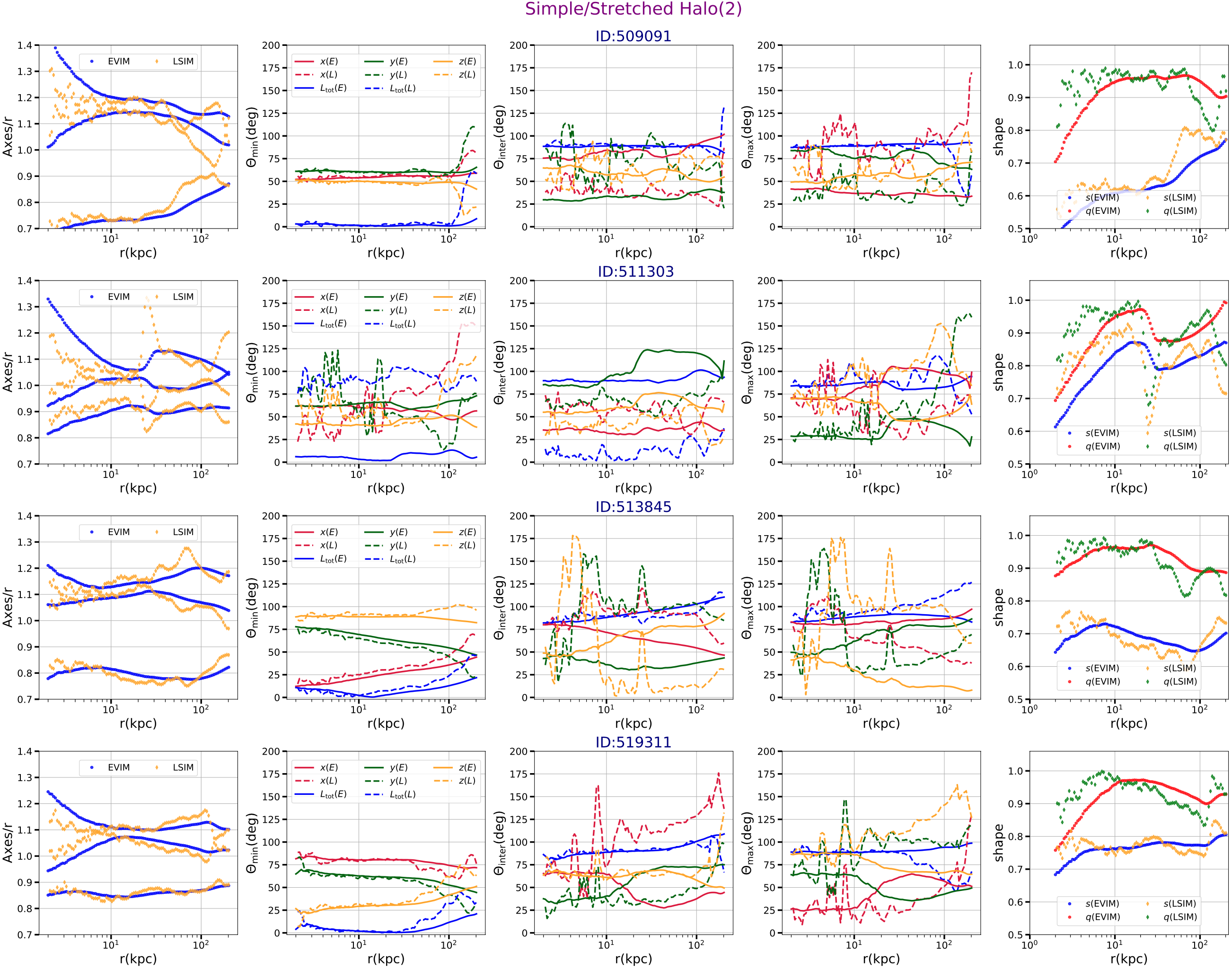
We start with analyzing the simple halos in our galaxy sample. Based on EVIM, such halos have two main properties; firstly, they have three well separated eigenvalues that the ordering in their magnitude does not change with radius and secondly, the eigenvector associated with the smallest eigenvalue is almost entirely parallel to the total angular momentum with little change in the angle. In addition, Other eigenvectors present rather small directional variations as well. There are in total 8 halos in this category. In Appendix C.1, we present the radial profile of the axes lengths, as well as the angles of eigenvectors associated with the minimum(min), intermediate(inter) and maximum(max) eigenvectors with different fixed vectors: (the angular momentum of the stellar component of the galaxy) and three unit vectors along the x,y,z directions of the TNG simulation box (refereed to as [, ]), and finally also the shape parameters for this group.
Although we take the EVIM as our main method, to check the robustness of the properties of the simple halos against using different methods, in Appendix C, we inferred the shape profiles using both of EVIM and LSIM. It is generally correct (with the exception of halo 511303) that the eigenvectors associated with the minimum eigenvalue are almost entirely parallel to the net angular momentum. However, owing to the local fluctuations, in some cases the lines do actually cross each other and a local rotation occurs. Owing to that, we may entitle these halos simple/stretched but just call them simple halos, as for abbreviation.
IV.2.2 Twisted halos
As the second class of halos, here we analyze the twisted halos. Halos belonging to this category show some level of rotation in the radial profile of their eigenvectors. To demonstrate such rotation, we compute the angle of min, inter and max eigenvectors with the aforementioned fixed vectors in 3D such as and . Twisted halos experience a gradual rotation of about 50-100 degs in their radial profile. Furthermore, their axes lengths get very close to each other, sometimes at the corner of crossing, but not really getting stretched, as is described below. There are 8 halos in this class. In appendix C.2 we summarize the radial profile of the axes lengths, different angles and shape profile of all of twisted halos.
As it was done in the case of simple halos, in Appendix C, we overlay the shape parameters from the LSIM. Generally speaking, the inferred halo shapes from EVIM and LSIM are fairly close to each other but only slightly noisier in LSIM because of the local fluctuations which may lead to extra crossings of the eigenvalues.
IV.2.3 Stretched halos
As the last class of halos, here we describe the stretched halos. Generally speaking, halos belong to this category experience a level of stretching in the radial profile of their axes lengths. Where two axes lengths approach each other and one of them stretches and gets larger than the other. Thanks to the orthogonality of eigenvectors, such stretching can be easily seen from changing the angle of min, inter and max eigenvectors with the aforementioned unit vectors [, ] by about 90 deg. Indeed, this criteria allows us to distinguish between the twisted and stretched halos. In summary, the crucial difference between the twisted and stretched halos is that former ones, twisted halos, establish a gradual changes in their angle while the latter one, stretched halos, show more of an abrupt changes in their angles.
In our galaxy sample, we have 9 halos in this category. In Appendix C.3 we summarize the radial profile of the axes lengths, different angles and shape profile of all of stretched halos.
Before we proceed with further study of halo properties in different classes, we shall mention that, there are two halos, halo 4 (ID: 480802) and halo 10 (ID: 501725), which show both of a twisting and stretching in their radial profiles at different radii. More explicitly, these halos demonstrate both of a gradual and abrupt changes throughout their radial profiles and when the principal axis lengths cross each other, respectively. To avoid further complexity of the presentation, however, we put them in the category of stretched halos throughout our following analysis.
As for the above two cases, in Appendix C.3, we also overlay the shape profiles from the LSIM. Quite interestingly, the general patterns from EVIM and LSIM are fairly close to each other with extra fluctuations that are arisen owing to the local fluctuations of the profiles.
Having introduced different classes of halos, in Figure 5 we present three halos, one from each category, and compare the radial profile of their axes lengths, angles with different vectors and their shape profiles. We use EVIM in our presentation. It is evident that the level of rotation in the simple halo is much less than the twisted and stretched halos. In addition, while twisted halo, show some level of gradual rotation throughout its radial profile, the stretched halo demonstrates a rotation of about 90 deg when the axes lengths cross each other.
IV.3 3D visualization of different halos:
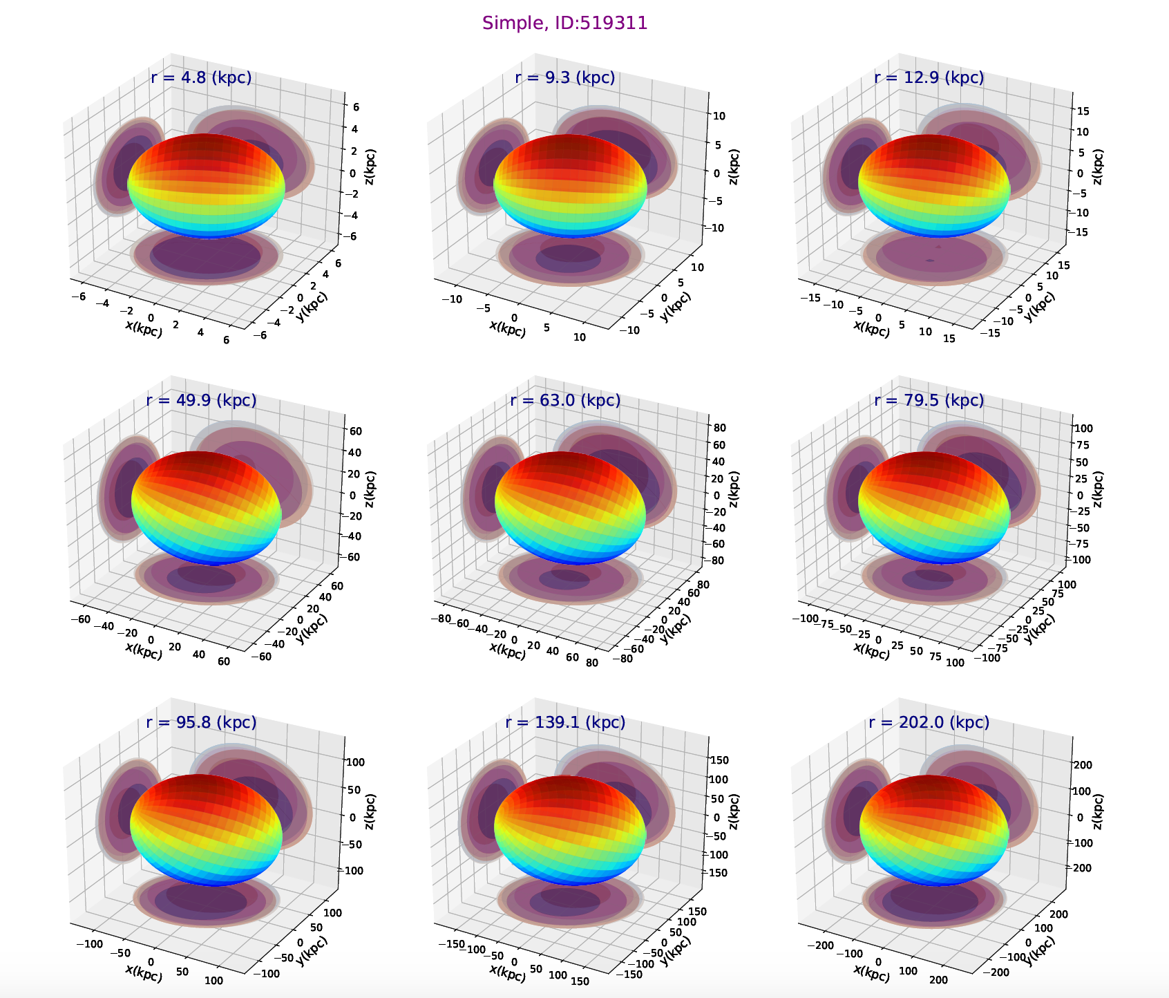
Having specified different halo types in our galaxy sample, here we aim to make a 3D visualization of their ellipsoidal profiles. In Figures 6-8, we draw 3D ellipsoids of simple, twisted and stretched halos at few different locations. To make each plot, we have ordered the eigenvalues and made a rotation from the principal frame to the Cartesian coordinate using the eigenvectors of the inertia tensor. In addition, at each plot, we also display the 2D projection of 3D ellipsoid in the XY, YZ and XZ planes. It is evident that while simple halo presents very little rotation, the twisted and stretched halos establish some level of rotation. In addition, while the twisted halo presents a gradual rotation, the stretched halo establishes a larger rotation near the crossing of the axes lengths.


IV.4 Halo shape and galaxy properties
Having presented different halo types, below we make the connection between the shape of halos and various galaxy properties such as the galaxy stellar mass as well as the halo formation time.
IV.4.1 Shape vs central galaxy stellar mass
Here we study the possible connection between the shape parameters and (central) galaxy stellar mass (hereafter galaxy stellar mass), . Table 4 presents the Spearman correlation between the shape parameters at and galaxy stellar mass, where we have chosen a physical distance to draw a better connection with the halo mass.
Before drawing any conclusions from the table, we should point out that owing to the small sample of simple, twisted and stretched halos, care must be taken in interpreting the statistical significance of these correlations. To take it into consideration, below we not only present the Spearman coefficient, Coeff, but we also report the p-value for every correlation. Furthermore, we name a correlation reliable if its p-value is less than 0.05. Having this said, it is clearly seen that only the correlation of () and for simple(twisted) halos are meaningful with a positive correlation. The correlation of () and for simple(twisted) halos are at the boundary of being reliable. However, the rest of correlations are not statistically reliable with having larger values of p-value.
In Figure 9, we find the correlation between and . From the plot, it is evident that stretched halos spans a narrower range of radii while simple and twisted halos spread over a wider range of masses and radii.
| Simple: | Coeff | -0.17 | 0.90 | -0.71 |
|---|---|---|---|---|
| p-value | 0.69 | 0.002 | 0.05 | |
| Twisted: | Coeff | -0.17 | 0.57 | -0.64 |
| p-value | 0.69 | 0.14 | 0.09 | |
| Stretched: | Coeff | -0.017 | 0.37 | -0.28 |
| p-value | 0.97 | 0.33 | 0.46 |
IV.4.2 Shape vs (stellar) halo formation time
Below, we make a possible connection between the shape parameters and the halo formation time (); defined as the time when the half of the galaxy stellar mass is formed. Table 5 presents the Spearman correlation between and . As we already mentioned in the correlation of the shape parameters and , due to the limited sample of halos in each category, we care must be taken in drawing any meaningful conclusions of the real correlation. Owing to this, we also report the p-value while presenting the correlation. As it turns out, the only meaningful correlation is between and in the stretched halos. However, we should emphasis here that the sample of stretched halos is very limited with only 5 halos. Being aware of this caveat, we conclude that in our galaxy samples, shape parameters do not seem to be correlated with the halo formation time.
Finally, it is interesting to make a possible connection between the halo mass and its formation time. Figure 10 presents the correlation between the galaxy stellar mass as well as the halo formation time. While the simple/twisted halos establish a positive correlation between and , stretched halos seem to indicate a rather flat correlation. Again we should keep in mind that the sample of stretched halos are a bit limited. Therefore care must be taken in drawing any strong conclusions here. Being mindful of the statistical caveat here, it might be that the nature of different halo types are a bit different. This suggests us to use larger box of TNG simulation and do the analysis for them as well. This is however beyond the scope of this work and is left to a future work. It is also interesting to make a connection between the halo shape and the merger trees. We leave this investigation to a future work as well.
| Simple: | Coeff | 0.32 | 0.22 | 0.12 |
|---|---|---|---|---|
| p-value | 0.43 | 0.61 | 0.78 | |
| Twisted: | Coeff | 0.048 | -0.44 | 0.24 |
| p-value | 0.91 | 0.27 | 0.57 | |
| Stretched: | Coeff | 0.45 | -0.62 | 0.70 |
| p-value | 0.23 | 0.07 | 0.04 |

V Main drivers of the shape
Having computed the shape of the DM halo in MW-like galaxies, below we study the impact of a few different drivers of the shape. Here we mainly focus on three different drivers including baryonic effects and the impact of substructures on halo morphology. In addition, we find the connection between the angular momentum of satellites and the eigenvectors of the reduced inertia tensor as well as .
V.1 Baryonic Effects: DMO simulations
One possible driver of DM halo shape is baryonic effects. Since baryonic contributions are generally very complex and hard to account for individually, to have an appropriate consideration of their possible impacts, we compute the shape of Dark Matter Only (DMO) simulations similar to Dubinski & Carlberg 1991; Warren et al. 1992; Jeeson-Daniel et al. 2011; Schneider et al. 2012; Chua et al. 2019. We then compare the final results with the estimated shape from the full hydrodynamical simulations.
We use TNG50-Dark and compute the shape of DMO MW-like halos. To match the halos from TNG50 to TNG50-Dark, we use the unique ID of dark matter particles. For every galaxy in our preselected sample, we scan the halos in DMO and look for a halo with highest fraction of matched DM particles. It is worth mentioning that TNG50 halos are less massive because of baryonic feedback processes, which eject some mass outside of the halo. This does not occur in the DMO simulation and thus halos in DMO are slightly more massive. To take this into account, in our matching, we take the mass range in TNG50-Dark to be slightly above the original selection in TNG50 as we also have put a prior choice on the range of halo mass to narrow down the interesting mass range a little bit. Therefore the matched DMO halos are found to be more massive; see Table 1 for more details. In most cases, the fraction of matched particles is more than 70%. In one case, though, 4th galaxy in the above sample, the percentage of matched DM particles was about 54%.
Before proceeding with the shape analysis, in Figure 11 we study the logarithm of the 2D projected (number) density of DM particles, in (x-y) plane, in a sample of 4 DMO halos of MW-like galaxies under consideration. Our chosen halos are associated with the matched cases to those in Figure 3. Each row presents one galaxy, with its given ID number, and from the left to right, we zoom-in further down to the central part of the halo. As expected, the halo structure varies for DMO case as compared with the DM profiles presented in Figure 3. Although all of the halos in our sample share the same gravity and subgrid baryonic physics, they differ in their formation histories. Owing to this, their density profile differs from each other. For example, the halo in the second row in Figure 3 is currently experiencing a halo merger.
In Figure 12 we draw the correlation between and ( as inferred from EVIM) at for both of TNG50 (Cen:left) versus TNG50-Dark (DMO:right). Where to distinguish between the central halo and FoF group that would be added later, we explicitly mention Cen here. Overlaid on the plots, are the scatter plot of the same quantities in both cases. It is evident that on average, central halos have larger values of and than DMO ones.
Figure 13 presents the radial profiles of the median and 16 (84) percentiles of for DMO simulations inferred using EVIM, LSNIM and LSIM. In contrast to the full-hydrodynamical simulation, here the inferred and from EVIM, LSIM have radially progressively increasing profiles. Consequently, the radial profile of the triaxiality parameter decreases in both approaches though its actual value is larger in DMO compared with the full-hydrodynamical simulations. In Table 6, we present the median and 16 (84) percentiles of the shape and triaxiality parameters. Comparing this with Table 3, it is evident that and are reduced while is increased (substantially) in DMO simulation (in EVIM).
| Method | |||
|---|---|---|---|
| EVIM | |||
| LSNIM | |||
| LSIM |
Our results suggest that baryonic effects make DM halos more oblate. This result are in great agreement with the conclusion of Chua et al. 2019. On the contrary, DM halo looks more prolate for DMO in all of these approaches at small radii and gets more triaxial/oblate at larger radii. Furthermore, is the largest in EVIM and smallest in LSNIM.
In conclusion, baryonic effects play a crucial contribution in shaping the DM halo in MW like galaxies.

V.2 Impact of FoF group on galaxy morphology
So far we only studied the impact of central halos in our analysis. Below we generalize our consideration and analyze the impact of different substructures, by using all particles associated with FoF groups in the shape of DM halo. This means that we analyze all particles, including the particles belonging to the central galaxy as well as substructures in our computations.
First, we study the impact of including all FoF particles on the projected density diagram. In Figure 14 we display the logarithm of the projected x-y (number) density profile for FoF group and a sub-sample of 4 galaxies of interest. As expected there are many substructures in the FoF. It is therefore intriguing how they could potentially affect the shape of the DM halo.
Having presented the central, DMO and FOF group, it is intriguing to compare their shape profiles. To facilitate the comparison, in Figures 15 and 16, we present the Axes/r ratio and the shape parameters in all of the above three cases. To make the plots easier to read, we only show the results from our main algorithm, EVIM.
Figure 15 presents the Axes/r ratio for a case of 3 MW-like galaxies in our galaxy sample. In each row, from left to right, we present Axes/r ratio for DM, FoF group, DMO and DMO (FoF) simulations. There are few take aways that can be inferred from the figure. First of all, it is evident that, in inner part of the halo, the impact of substructures is subdominant for both of the hydro and DMO simulations. Next, the radial profile of Axes/r ratio are largely different between the full hydro and DMO simulations. This brings us to the picture that baryonic effects are more important in shaping the halos than the current substructures.
Figure 16 shows the radial profile of the shape parameters for a sample of 3 MW like galaxies from our sample. Overlaid on every plot, we present the shape for DM, FoF group, DMO and DMO (FoF) simulations. The shape profile of FoF group is fairly close to the case of DM halo in the inner part of halo, up to 100 kpc. On the contrary, DMO simulation predicts a somewhat smaller value for the shape parameters.
V.3 Connection with Satellites
Having presented the Milky Way like galaxies as central subhalos in every group, here we discuss the satellites in individual galaxies. Satellite galaxies are associated with the subhalos which are themselves the members of their parent FoF halo. In IllustrisTNG simulations, subhalos are ordered in terms of their masses, with heaviest member at the beginning of every group identified as the central galaxy; while the rest are assigned as satellites.
We adopt a stellar mass cut, hereafter , in the mass range to ensure that we study subhalos with more than stellar particles taking into account that the unit mass of baryons in TNG50 is . In addition, we restrict ourselves to distances less than 200 kpc. Furthermore, we also eliminate satellites that do not have a cosmological origin. In the TNG simulation, it is done by checking the “SubhaloFlag”.
In Figure 17, we present the number of satellites within the above mass and distance ranges as the function of their median distance from the halo center. While more than the half of the satellites of simple and twisted halos are in average closer than 125 kpc, those associated with the stretched halo are mostly farther out. Furthermore, stretched halos have slightly less satellites compared with the simple and twisted halos. Therefore, care must be taken when we draw a statistical conclusion about the current sample.
In Figures 18-20 we study the 2D distribution of the angle between the angular momentum of satellites and the closest eigenvectors associated with the minimum-to-maximum eigenvalues. Also to compute and track the angle profiles, we propose for the angles to be initially less than 90 deg. In each figure, from the left to right, we draw the 2D distribution of all, simple, twisted and stretched halos, respectively. There are few interesting take aways points from the above analysis:
In Simple halos, the angular momentum of satellites is more aligned with the minimum eigenvector than the other two classes.
In twisted and stretched halos, there is a bi-modality in the distribution of the angular momentum of satellites and the minimum eigenvectors computed at different locations. Where almost a half of satellites are anti-aligned (with the angles around 180 deg) with the minimum eigen-vector, while the rest of them are in a similar range of angles to those associated with simple halos.
There is also a bi-modality in the radial distribution of the satellites of simple and twisted halos. In particular, almost half of them are located closer than 100 kpc, while the rest are between 100 to 200 kpc.
While the angle profiles of the angular momentum of satellites and the minimum eigenvectors are peaked at around 40 deg, the radial profile of all of angular momentum of satellites with the intermediate and maximum eigenvectors peak at around 70 deg and 80 deg, respectively. This means that satellites are generally in more aligned with the minimum eigenvector than the intermediate and maximum ones.
Next, in Figure 21 we study the 2D distribution of the angle between the angular momentum of satellites and . From the left to right, we present all, simple, twisted and stretched halos, respectively.
From the plot, it is inferred that in the simple and twisted halos, mostly grow from left to right where closer by satellites are being more aligned with the than those farther out. There are however few cases where simple/twisted halos are anti-aligned with the . On the contrary, in the stretched halos, seems to have a flat distribution.
Finally, in Figures 22-23, we present the 2D and 1D distribution of the infall redshift vs the radius and infall redshift for satellites of different halo types. To infer the satellite’s infall-time, we trace each of them backward in time down to the redshift where prior to this, the satellite does not belong to the central halo.
From Figure 22, it is inferred that, for simple and stretched halos, the infall-time is mostly between z = 0.3-1.0 and less than 25% of satellites being accreted before . However, in twisted halos, there are some bi-modalities in the distribution of the infall-time of satellites with about 39% of them being accreted at . Such bi-modality is seen as the little bump in the 1D distribution of the satellite’s infall-time from Figure 23. Again we should note that since the current sample is limited, care should be taken in any statistical conclusions!


VI Connection to observations
Thus far we assessed the shape of DM halo in MW like galaxies in TNG50 using different techniques. Below we connect these theoretical outcomes to recent observational constraints on these shapes. Furthermore, since the radial distribution of shape parameters are rather different between different techniques, we may be able to distinguish between them as well.
Observationally, one may indicate the shape of DM halo without directly measuring this in MW galaxy. Below, we use the observational constraints on the shape of DM halos as provided in Bland-Hawthorn & Gerhard 2016 and references therein.
One possible way to determine the DM halo shape in the MW is using the orbit of Sgr dwarf across the sky. It was shown that the geometry of the stream across the sky confirms an oblate to near spherical DM halo (Ibata et al. 2001; Johnston et al. 2005). More specifically, Johnston et al. 2005 used radial velocities of a sample of (few)-hundred M giant candidates from Two Micron All Sky Survey (2MASS) catalog to trace streams of tidal debris associated with Sagittarius dwarf spheroidal galaxy (Sgr) which entirely encircle MW Galaxy. They strongly favoured an iso-density at the distance between 13-60 kpc and ruled out and at 3. It is important to note that while for triaxial halos, both of shape parameters are by definition less than unity, in the context of axisymmetric halos, where the density profile is a function of , the flattening parameter can be smaller/larger than unity for the oblate/prolate halos. Therefore, we make a transformation between axisymmetric parameter (hereafter ) and our triaxial based results. Below, we make the following transformation. If the is larger than one, we read and if the is less than one, we shall take while .
Later, Helmi 2004 used line-of-sight velocities and compared the kinematics of Johnston et al. 2005 M giant sample to the models of Sgr dwarf debris and showed that a portion of mapped trailing stream is dynamically young and thus does not imply a strong constraint of the shape. On the other hand, the leading stream consists of older debris and its dynamics provides a strong indication towards a prolate halo shape with .
Kalberla et al. 2007 used data from Leiden-Argentine-Bonn all sky 21-cm line survey and derived the 3D density distribution for MW to constrain the galactic mass distribution. They found a majority of DM particles can be modeled using an isothermal disk within kpc. Though the confirmation of DM disk is a hint for an oblate shape, they showed that a halo with a constant does not quite match with the observations and that the halo shape should be progressively prolate at larger distances.
Koposov et al. 2010 combined SDSS photometry, USNO-B astrometry and SDSS/Calar Alto spectroscopy and constructed an empirical 6D phase-space map of GD-1 stream of stars located at 15 kpc from the galactic center and is believed to be debris from a tidally disrupted star cluster. Using an axisymmetric potential, made of stellar disk and DM halo, they found , at the Galactocentric radii near to 15 kpc; where refers to the flattening in DM gravitational potential.
Garbari et al. 2012 used the kinematic and position data for K dwarf stars located near the sun in a distance less than 1.1 kpc from the galactic plane from (Kuijken & Gilmore 1989) and determined the DM halo density in the MW. They reported a mild tension with the assumption of a spherical halo but consistent with an oblate DM halo with or a local disc or a spherical DM halo with larger normalization.

Küpper et al. 2015 used the tidal streams from Palomar5 (Pal5), the faintest and most extended, globular cluster in the MW. They estimated the DM halo shape to be nearly spherical with a potential flattening at the heliocentric distance 23.6 kpc. Using the proper motion of 75 globular clusters in Gaia DR2, Posti & Helmi 2019 estimated the mass and axis ratio of DM within kpc. They reported a prolated DM halo with . This rules out very oblate DM halo with and very prolated halo with at 3.
Figure 24 summarizes the above constraints on the shape parameters of the DM halo. Overlaid on the plot are the medians of EVIM, LSNIM and LSIM for both of Cen and DMO simulations. We shall emphasize that all of the y-axes are located at , the slight displacement is for the clarity of the presentation. Out results are comparable with most of these results. The level of the agreement between the simulations ans observational results are indeed excellent.
VII Summary and conclusion
In this paper, we used the hydrodynamic simulation of TNG50 and extracted a sample of 25 MW like galaxies identified using two different criteria. The first criterion is that the DM halo is belong to a mass range of to . The second is that the disk-frac, defined as the fraction of number of stars with orbital circularity parameter, , is above 40%. We computed the radial profile of shape parameters for DM halo. We exploited three different approaches in our shape analysis. In the first approach, we inferred the halo shape using an enclosed volume iterative method, EVIM. In the second approach, we computed the shape using a local shell non-iterative method, LSNIM. Finally, in the third approach, we calculated the shape using a local in shell iterative method, LSIM.
The radial profile of the is fairly similar between EVIM, LSIM in the inner part of the halo but slightly deviates after the radius of 80 kpc. On the contrary,, LSNIM predicts a larger profile for parameter which is progressively diminishing from the inner to the outer part of the halo. On the other hand, the radial profile of the is very close between EVIM, LSIM up to 10 kpc with a switch over behavior at larger radii where EVIM gets closer to the LSNIM than LSIM.
Based on our shape analysis which are mainly taken from EVIM, we classify DM halos in our galaxy sample into 3 main categories. Simple halos develop well separated eigenvalues that never cross each other (based on EVIM). But,owing to the local fluctuations, they could pass through each other in LSIM. However, since our halo classification is based on the EVIM, name this class as simple halos. Furthermore, the eigenvector associated with the minimum eigenvalue in these halos is almost entirely parallel to . There are in total 8 halos in this class.
Twisted halos establish some level of gradual rotation throughout their radial profile. The level of reorientation varies from one halo to the other but in general the halo is reoriented in this radial profile. There are in total 8 halos in this class of halos.
Stretched halos experience some levels of stretching (even in EVIM) in their radial profiles, where different eigenvalues cross each other. Consequently, the angle of their corresponded eigenvectors with different vectors varies by 90 deg at the location of stretching, thanks to the orthogonality of different eigenvectors. There are in total 9 different halos in this category.
We drew 3D ellipsoids for each category and established the rotation in the halo radial profile for each part.
We studied the main drivers of the DM halo shape. In this first study, we focused on three different drivers including the baryonic effects, impact of substructures. For the first driver, we computed the halo shape in dark matter only (DMO) simulations. We measured a smoother radial profile for with a triaxial/prolate halo shape. This means that baryonic effects tend to decrease the diskyness of halos. Remarkably, in DMO simulation, and are increasing with the radius. Accordingly, is decreasing for both approaches. Our analysis showed that halos are more simple in DMO than the full hydro-simulation. This is suggestive and indicates that twisted/stretched halos may have some baryonic reasons. Work is in progress to study these features in more details.
We examined the effect of substructures in the shape in both of full hydro-simulation and DMO simulations. Our analysis shows that in most cases the impact of substructures in the shape are subdominant in the inner part of the halo.
Furthermore, we also studied the location and angular momentum of MW satellites in the mass range and at the distance less than 200 kpc. We computed the radial profile of the angle between the angular momentum of satellites and min,inter, max eigenvectors. Our analysis show that the satellites of simple halos are more aligned with the minimum eigenvector than the other two classes. Furthermore, in twisted and stretched halos, instead, there is a bi-modality in the distribution of the angular momentum of the satellites and the closest minimum eigenvector.
Furthermore, the distribution of the infall time of satellites shows that the majority of them is accreted onto the main halo between .
Finally, we connected our theoretical predictions for shape parameters to some of the recent observational studies. We overlaid our theoretical results on the top of few well studied tracers such as stream of tidal debris, GD-1 stream of stars, K dwarf stars and globular clusters from Gaia DR2 and found a fairly good agreement. In a companion paper, we aim to make a comprehensive study of the remaining possible drivers in the halo shapes.
Since the radial profile of the shape parameters are not the same, we may hope that more detailed observations at different radii distinguish between different methods. For instance, it would be fascinating to use the spectroscopic data from Hectochelle in the Halo at High Resolution (H3) survey (Conroy et al. 2019) and compute the radial dependence of the shape for DM halo.
Throughout this work, we only studied the shape of the DM halo. In Emami et al. 2020, we generalize this study to the case of Stellar halo and their possible connection to that of DM shape as studied here.
Data Availability
Data directly related to this publication and its figures is available on request from the corresponding author. The IllustrisTNG simulations themselves are publicly available and accessible at www.tng-project.org/data (Nelson et al. 2019), where the TNG50 simulation will also be made public in the future.
acknowledgement
It is a great pleasure to thank David Barnes, Angus Beane, Ana Bonaca, Dylan Nelson, Sandro Tacchella, Matthew Smith, and Annalisa Pillepich for the very insightful conversations. We especially acknowledge Charlie Conroy for his assistance with making the connection to observations. We thank the referee for their constructive comments that improved the quality of this paper. R.E. acknowledges the support by the Institute for Theory and Computation at the Center for Astrophysics. We thank the supercomputer facility at Harvard where most of the simulation work was done. MV acknowledges support through an MIT RSC award, a Kavli Research Investment Fund, NASA ATP grant NNX17AG29G, and NSF grants AST-1814053, AST-1814259 and AST-1909831. SB is supported by Harvard University through the ITC Fellowship. FM acknowledges support through the Program ”Rita Levi Montalcini” of the Italian MIUR. The TNG50 simulation was realized with compute time granted by the Gauss Centre for Supercomputing (GCS) under GCS Large-Scale Projects GCS-DWAR on the GCS share of the supercomputer Hazel Hen at the High Performance Computing Center Stuttgart (HLRS).
Software: matplotlib (Hunter 2007), numpy (van der Walt et al. 2011), scipy (Oliphant 2007), seaborn (Waskom et al. 2020), pandas (McKinney, Wes et.al), h5py (De Buyl et al. 2016).
References
- Abadi et al. (2003) Abadi, M. G., Navarro, J. F., Steinmetz, M., et al. 2003, ApJ, 591, 499
- Abadi et al. (2010) Abadi, M. G., Navarro, J. F., Fardal, M., et al. 2010, MNRAS, 407, 435
- Allgood et al. (2006) Allgood, B., Flores, R. A., Primack, J. R., et al. 2006, MNRAS, 367, 1781
- Bailin & Steinmetz (2005) Bailin, J., & Steinmetz, M. 2005, ApJ, 627, 647
- Barnes & Efstathiou (1987) Barnes, J., & Efstathiou, G. 1987, ApJ, 319, 575
- Bland-Hawthorn & Gerhard (2016) Bland-Hawthorn, J., & Gerhard, O. 2016, ARA&A, 54, 529
- Brammer et al. (2012) Brammer, G. B., van Dokkum, P. G., Franx, M., et al. 2012, ApJS, 200, 13
- Buck et al. (2018) Buck, T., Macciò, A., Ness, M., et al. 2018, Rediscovering Our Galaxy, 209
- Buck et al. (2020) Buck, T., Obreja, A., Macciò, A. V., et al. 2020, MNRAS, 491, 3461
- Butsky et al. (2016) Butsky, I., Macciò, A. V., Dutton, A. A., et al. 2016, MNRAS, 462, 663
- Camps & Baes (2015) Camps, P., & Baes, M. 2015, Astronomy and Computing, 9, 20
- Chua et al. (2019) Chua, K. T. E., Pillepich, A., Vogelsberger, M., et al. 2019, MNRAS, 484, 476
- Conroy et al. (2019) Conroy, C., Bonaca, A., Cargile, P., et al. 2019, ApJ, 883, 107
- Crain et al. (2015) Crain, R. A., Schaye, J., Bower, R. G., et al. 2015, MNRAS, 450, 1937
- Davis et al. (1985) Davis, M., Efstathiou, G., Frenk, C. S., et al. 1985, ApJ, 292, 371
- De Buyl et al. (2016) de Buyl, P., Huang, M.-J., & Deprez, L. 2016, arXiv e-prints, arXiv:1608.04904
- Dolag et al. (2009) Dolag, K., Borgani, S., Murante, G., et al. 2009, MNRAS, 399, 497
- Dubinski & Carlberg (1991) Dubinski, J., & Carlberg, R. G. 1991, ApJ, 378, 496
- Dubinski (1994) Dubinski, J. 1994, ApJ, 431, 617
- Eisenstein & Loeb (1995) Eisenstein, D. J., & Loeb, A. 1995, ApJ, 439, 520
- El-Badry et al. (2018) El-Badry, K., Quataert, E., Wetzel, A., et al. 2018, MNRAS, 473, 1930
- Emami et al. (2020) Emami R., Hernquist L., Alcock C., Genel S., Bose S., Weinberger R., Vogelsberger M., et al., 2020, arXiv, arXiv:2012.12284
- Erkal et al. (2019) Erkal, D., Belokurov, V., Laporte, C. F. P., et al. 2019, MNRAS, 487, 2685
- Font et al. (2020) Font, A. S., McCarthy, I. G., Poole-Mckenzie, R., et al. 2020, arXiv e-prints, arXiv:2004.01914
- Garbari et al. (2012) Garbari, S., Liu, C., Read, J. I., et al. 2012, MNRAS, 425, 1445
- Garrison-Kimmel et al. (2018) Garrison-Kimmel, S., Hopkins, P. F., Wetzel, A., et al. 2018, MNRAS, 481, 4133
- Genel et al. (2014) Genel, S., Vogelsberger, M., Springel, V., et al. 2014, MNRAS, 445, 175
- Gómez et al. (2017) Gómez, F. A., White, S. D. M., Grand, R. J. J., et al. 2017, MNRAS, 465, 3446
- Grand et al. (2018) Grand, R. J. J., Helly, J., Fattahi, A., et al. 2018, MNRAS, 481, 1726
- Grogin et al. (2011) Grogin, N. A., Kocevski, D. D., Faber, S. M., et al. 2011, ApJS, 197, 35
- Hani et al. (2019) Hani, M. H., Ellison, S. L., Sparre, M., et al. 2019, MNRAS, 488, 135
- Helmi (2004) Helmi, A. 2004, ApJ, 610, L97
- Hunter (2007) Hunter, J. D. 2007, Computing in Science and Engineering, 9, 90
- Ibata et al. (2001) Ibata, R., Lewis, G. F., Irwin, M., et al. 2001, ApJ, 551, 294
- Jeeson-Daniel et al. (2011) Jeeson-Daniel, A., Dalla Vecchia, C., Haas, M. R., et al. 2011, MNRAS, 415, L69
- Jing & Suto (2002) Jing, Y. P., & Suto, Y. 2002, ApJ, 574, 538
- Johnston et al. (2005) Johnston, K. V., Law, D. R., & Majewski, S. R. 2005, ApJ, 619, 800
- Kalberla et al. (2007) Kalberla, P. M. W., Dedes, L., Kerp, J., et al. 2007, A&A, 469, 511
- Kazantzidis et al. (2004) Kazantzidis, S., Kravtsov, A. V., Zentner, A. R., et al. 2004, ApJ, 611, L73
- Koekemoer et al. (2011) Koekemoer, A. M., Faber, S. M., Ferguson, H. C., et al. 2011, ApJS, 197, 36
- Koposov et al. (2010) Koposov, S. E., Rix, H.-W., & Hogg, D. W. 2010, ApJ, 712, 260
- Kuijken & Gilmore (1989) Kuijken, K., & Gilmore, G. 1989, MNRAS, 239, 605
- Küpper et al. (2015) Küpper, A. H. W., Balbinot, E., Bonaca, A., et al. 2015, ApJ, 803, 80
- Lambas et al. (1992) Lambas, D. G., Maddox, S. J., & Loveday, J. 1992, MNRAS, 258, 404
- Law & Majewski (2010) Law, D. R., & Majewski, S. R. 2010, ApJ, 714, 229
- Marinacci et al. (2018) Marinacci, F., Vogelsberger, M., Pakmor, R., et al. 2018, MNRAS, 480, 5113
- (47) McKinney, W. et al. Proceedings of the 9th Python in Science Conference, 445, 51-56, 2010
- Merritt et al. (2020) Merritt, A., Pillepich, A., van Dokkum, P., et al. 2020, MNRAS, doi:10.1093/mnras/staa1164
- Monachesi et al. (2016) Monachesi, A., Gómez, F. A., Grand, R. J. J., et al. 2016, MNRAS, 459, L46
- Monachesi et al. (2019) Monachesi, A., Gómez, F. A., Grand, R. J. J., et al. 2019, MNRAS, 485, 2589
- Naiman et al. (2018) Naiman, J. P., Pillepich, A., Springel, V., et al. 2018, MNRAS, 477, 1206
- Nelson et al. (2018) Nelson, D., Pillepich, A., Springel, V., et al. 2018, MNRAS, 475, 624
- Nelson et al. (2019) Nelson, D., Pillepich, A., Springel, V., et al. 2019, MNRAS, 490, 3234
- Nelson et al. (2019) Nelson, D., Springel, V., Pillepich, A., et al. 2019, Computational Astrophysics and Cosmology, 6, 2
- Oliphant (2007) Oliphant, T. E. 2007, Computing in Science and Engineering, 9, 10
- Orr et al. (2019) Orr, M. E., Hayward, C. C., Medling, A. M., et al. 2019, arXiv e-prints, arXiv:1911.00020
- Pandya et al. (2019) Pandya, V., Primack, J., Behroozi, P., et al. 2019, MNRAS, 488, 5580
- Pillepich et al. (2018) Pillepich, A., Nelson, D., Hernquist, L., et al. 2018, MNRAS, 475, 648
- Pillepich et al. (2018) Pillepich, A., Springel, V., Nelson, D., et al. 2018, MNRAS, 473, 4077
- Pillepich et al. (2019) Pillepich, A., Nelson, D., Springel, V., et al. 2019, MNRAS, 490, 3196
- Planck Collaboration et al. (2016) Planck Collaboration, Ade, P. A. R., Aghanim, N., et al. 2016, A&A, 594, A13
- Posti & Helmi (2019) Posti, L., & Helmi, A. 2019, A&A, 621, A56
- Prada et al. (2019) Prada, J., Forero-Romero, J. E., Grand, R. J. J., et al. 2019, MNRAS, 490, 4877
- Ravindranath et al. (2006) Ravindranath, S., Giavalisco, M., Ferguson, H. C., et al. 2006, ApJ, 652, 963
- Rodríguez-Puebla et al. (2013) Rodríguez-Puebla, A., Avila-Reese, V., & Drory, N. 2013, ApJ, 773, 172
- Rodriguez-Gomez et al. (2019) Rodriguez-Gomez, V., Snyder, G. F., Lotz, J. M., et al. 2019, MNRAS, 483, 4140
- Sandage et al. (1970) Sandage, A., Freeman, K. C., & Stokes, N. R. 1970, ApJ, 160, 831
- Sanderson et al. (2020) Sanderson, R. E., Wetzel, A., Loebman, S., et al. 2020, ApJS, 246, 6
- Santistevan et al. (2020) Santistevan, I. B., Wetzel, A., El-Badry, K., et al. 2020, arXiv e-prints, arXiv:2001.03178
- Schaye et al. (2015) Schaye, J., Crain, R. A., Bower, R. G., et al. 2015, MNRAS, 446, 521
- Schneider et al. (2012) Schneider, M. D., Frenk, C. S., & Cole, S. 2012, J. Cosmology Astropart. Phys, 2012, 030
- Schinnerer et al. (2013) Schinnerer, E., Meidt, S. E., Pety, J., et al. 2013, ApJ, 779, 42
- Shao et al. (2020) Shao, S., Cautun, M., Deason, A. J., et al. 2020, arXiv e-prints, arXiv:2005.03025
- Sijacki et al. (2015) Sijacki, D., Vogelsberger, M., Genel, S., et al. 2015, MNRAS, 452, 575
- Skelton et al. (2014) Skelton, R. E., Whitaker, K. E., Momcheva, I. G., et al. 2014, ApJS, 214, 24
- Springel et al. (2001) Springel, V., White, S. D. M., Tormen, G., et al. 2001, MNRAS, 328, 726
- Springel et al. (2004) Springel, V., White, S. D. M., & Hernquist, L. 2004, Dark Matter in Galaxies, 421
- Springel (2010) Springel, V. 2010, MNRAS, 401, 791
- Springel et al. (2018) Springel, V., Pakmor, R., Pillepich, A., et al. 2018, MNRAS, 475, 676
- Tenneti et al. (2015) Tenneti, A., Mandelbaum, R., Di Matteo, T., et al. 2015, MNRAS, 453, 469
- Thomas et al. (1998) Thomas, P. A., Colberg, J. M., Couchman, H. M. P., et al. 1998, MNRAS, 296, 1061
- Trayford et al. (2019) Trayford, J. W., Frenk, C. S., Theuns, T., et al. 2019, MNRAS, 483, 744
- van der Walt et al. (2011) Van der Walt, S., Colbert, S. C., & Varoquaux, G. 2011, Computing in Science and Engineering, 13, 22
- van der Wel et al. (2014) Van der Wel, A., Chang, Y.-Y., Bell, E. F., et al. 2014, ApJ, 792, L6
- Vogelsberger et al. (2014a) Vogelsberger, M., Genel, S., Springel, V., et al. 2014, MNRAS, 444, 1518
- Vogelsberger et al. (2014b) Vogelsberger, M., Genel, S., Springel, V., et al. 2014, Nature, 509, 177
- Vogelsberger et al. (2020) Vogelsberger, M., Marinacci, F., Torrey, P., et al. 2020, Nature Reviews Physics, 2, 42
- Warren et al. (1992) Warren, M. S., Quinn, P. J., Salmon, J. K., et al. 1992, ApJ, 399, 405
- Waskom et al. (2020) Waskom, M., Botvinnik, O., Ostblom, J., et al. 2020, mwaskom/seaborn: v0.10.0 (January 2020), v0.10.0, Zenodo, doi:10.5281/zenodo.3629446
- Weinberger et al. (2017) Weinberger, R., Springel, V., Hernquist, L., et al. 2017, MNRAS, 465, 3291
- Zhang et al. (2019) Zhang, H., Primack, J. R., Faber, S. M., et al. 2019, MNRAS, 484, 5170
- Zhu et al. (2016) Zhu, Q., Marinacci, F., Maji, M., et al. 2016, MNRAS, 458, 1559
Appendix A Non-Disky galaxies
As the main focused of this paper, so far we merely studied the disky MW like galaxies with more than 40% of stars living in the disk, defined with . From Figure 1 we inferred a very similar distribution for the orbital circularity parameter. In this appendix, we proceed further and study the distribution of the orbital circularity parameter for a sub-sample of galaxies with less fraction of stars living in the disk. In Figure 25 we present the distribution of for 4 galaxies with the mass similar to the MW galaxy. On the top of each plot, we labeled the Disk-frac. The plot considers 4 different Disk-fracs: .
Unlike the case of disky MW like galaxies with very similar distribution, here the distribution of varies a lot between different galaxies. It will be interesting to compute the shape for these non-disky galaxies. This analysis is however beyond the scope of this work and is left to a future study.
Appendix B Convergence Check for shape analysis
As already mentioned in Sec. III.1, our first shape finder algorithm, EVIM, relies on an iterative approach in which the algorithm is stopped after the shape parameters are converged such that max where and refer to the residual of the shape parameters . Here we describe in more detail how the convergence is established in our approach. Furthermore, as a sanity check, we will also present few examples with progressive reduction of the residuals from the above algorithm.
The convergence check in our shape finder algorithm proceed as follows. First, we leave the system for at least 12 iterations before proposing any convergence criteria. This allows the system to get stabilized since its first couple of iterations are required to get deviated from the initially proposed spherical symmetry. Then, to make sure that the convergence has truly established, we do not terminate the iteration once we get below the above threshold but allow the system to proceed and wait for having at least 15 consecutive cases with the residual below . Since at every iteration the spheroid is getting deformed, it may well happen that the system experiences some sudden jumps and the residual increases from one iteration to the other. If that occurs, we will set the counter to zero and again seek for 15 consecutive cases below the above threshold. This is very ensuring condition and in most cases reduce the residual substantially below .
Appendix C Halo Classification
As already mentioned in the main text, based on our shape analysis, we can identify different halo types; the so called simple, twisted and stretched halos. Here we present the radial profile of the Axes/r ratio, the angle of min-inter-max eigenvectors with the unit vectors along the x, y, z directions of the simulation box and the shape profile for all of 25 halos in our galaxy sample.
Furthermore, in order to have unambiguous association of angles at the initial point and avoid the possibility of the exchange of angles from very small to close to 180, we propose that all of the angles are initially less than 90 deg. Depending on the halo type, some of these angles could grow and get bigger than 90 deg throughout their radial profiles. This is done by simply making a mask over the angle associated with the initial location and apply this to the entire radial profile of the angles.
C.1 Profile of simple/Stretched halos
We start with the simple halo class. In Figures 26-27, we present the radial profile of Axes/r, angles and shape parameters for this type. Overlaid on each figure, we also present the results from the LSIM method. Quite remarkably, the results of EVIM for the Axes/r and shape parameters are fairly close to that of LSIM. However, since LSIM is sensitive to the local details of the shape, it is seen that there are some extra crossing of lines from LSIM which leads to some extra rotations in LSIM. Because of this, in LSIM, we name this class as simple/stretching. However, as we take EVIM as the main method, to simplify the classification, we call this group as simple halos. The results of EVIM explicitly show that the level of halo rotation is very minimal. There are in total 8 halos in this category.

C.2 Profile of twisted halos
Next, we study the twisted halos. In Figures 28-29, we analyse the radial profile of Axes/r, angles and shape parameters for this type. It is evident that halos in this category experience some gradual level of rotations from 50 to 100 degs in their radial profiles. There are in total 8 halos in this category. Overlaid on each figure, we also present the results from the LSIM. Interestingly, the outcome of EVIM and LSIM are fairly close to each other.


C.3 Profile of stretched halos
Finally, we analyse the stretched halos. In Figures 30-31, we analyse the radial profile of Axes/r, angles and shape parameters for this type. Halos in this category, experience one (or more) stretching where different eigenvalues cross each other. Consequently, the halo experience a change of angle of order 90 deg at the location of stretching. There are in total 9 halos in this class of halos. Overlaid on each figure, we also present the results from the LSIM. Interestingly, the outcome of EVIM and LSIM are fairly close to each other.


Appendix D Impact of weighting factor in the shape
Having presented different methods in analysing the DM halo shape, here we make a final comparison between these methods. Since the inertia tensor depends on the weighting factor, here we check the impact of different choices in the final shape. In Figure 32, we examine the impact of and unity weighting factors in LSIM in the shape parameters. Overlaid on the figure, we also present the results from the EVIM. It is evident that the results of the LSIM from the above two choices of the weighting factors are almost the same. This is reasonable since we are dealing with very thin shells where the elliptical radii is almost one.