A Bayesian Time-Varying Effect Model for Behavioral mHealth Data
The integration of mobile health (mHealth) devices into behavioral health research has fundamentally changed the way researchers and interventionalists are able to collect data as well as deploy and evaluate intervention strategies. In these studies, researchers often collect intensive longitudinal data (ILD) using ecological momentary assessment methods, which aim to capture psychological, emotional, and environmental factors that may relate to a behavioral outcome in near real-time. In order to investigate ILD collected in a novel, smartphone-based smoking cessation study, we propose a Bayesian variable selection approach for time-varying effect models, designed to identify dynamic relations between potential risk factors and smoking behaviors in the critical moments around a quit attempt. We use parameter-expansion and data-augmentation techniques to efficiently explore how the underlying structure of these relations varies over time and across subjects. We achieve deeper insights into these relations by introducing nonparametric priors for regression coefficients that cluster similar effects for risk factors while simultaneously determining their inclusion. Results indicate that our approach is well-positioned to help researchers effectively evaluate, design, and deliver tailored intervention strategies in the critical moments surrounding a quit attempt.
,
,
,
and
Colorado State University??, Oklahoma Tobacco Research Center??and Rice University??
1 Introduction
1.1 Scientific Background
The integration of mobile health (mHealth) devices into behavioral health research has fundamentally changed the way researchers and interventionalists are able to collect data as well as deploy and evaluate intervention strategies. Leveraging mobile and sensing technologies, just-in-time adaptive interventions (JITAI) or ecological momentary interventions are designed to provide tailored support to participants based on their mood, affect, and socio-environmental context (Heron and Smyth 2010; Nahum-Shani et al. 2017). In order to deliver theory-based interventions at critical moments, researchers collect intensive longitudinal data using ecological momentary assessment (EMA) methods, which aim to capture psychological, emotional, and environmental factors that may relate to a behavioral outcome in near real-time. In practice, JITAIs’ effectiveness depends on accurately identifying high-risk situations by the user or by pre-determined decision rules to initiate the delivery of intervention components. Decision rules for efficacious interventions rely on a thorough understanding of the factors that characterize a subject’s risk for a behavioral outcome, the dynamics of these risk factors’ relation with the outcome over time, and the knowledge of possible strategies to target a risk factor (Nahum-Shani et al. 2017).
In the analysis of this paper, we investigate a behavioral health intervention study that targets smoking cessation. Historically, smoking cessation studies have used health behavior theory (Shiffman et al. 2002; Timms et al. 2013) or group-level trends of smoking antecedents (Piasecki et al. 2013) to determine when a JITAI should be triggered. However, this approach is limited since current health behavior models are inadequate for guiding the dynamic and granular nature of JITAIs (Riley et al. 2011; Klasnja et al. 2015). Additionally, the design of efficacious smoking cessation interventions is challenged by the complexity of smoking behaviors around a quit attempt and misunderstandings of the addiction process (Piasecki et al. 2002). More recently, smoking behavior researchers have capitalized on the ability of mHealth techniques to collect rich streams of data capturing subjects’ experiences close to their occurrence at a high temporal resolution. The structure, as well as the complexity, of these data provide unique opportunities for the development and implementation of more advanced analytical methods compared to traditional longitudinal data analysis methods used in behavioral research (e.g., mixed models, growth curve models) (Trail et al. 2014). For example, researchers have applied reinforcement learning (Luckett et al. 2019) and dynamic systems approaches (Trail et al. 2014; Rivera, Pew and Collins 2007; Timms et al. 2013) to design and assess optimal treatment strategies using mHealth data. Additionally, Koslovsky et al. 2018, de Haan-Rietdijk et al. 2017 and Berardi et al. 2018 have applied hidden and observed Markov models to study transitions between discrete behavioral states, Shiyko et al. 2012 and Dziak et al. 2015 have used mixture models to identify latent structures, and Kürüm et al. 2016 have employed joint modeling techniques to study the complexity of smoking behaviors.
Greater insights into the dynamic relation between risk factors and smoking behaviors have been generated by the application of functional data techniques (Trail et al. 2014; Vasilenko et al. 2014; Koslovsky et al. 2017; Tan et al. 2012). These methods are well-suited for high-dimensional data with unbalanced and unequally-spaced observation times, matching the format of data collected with EMAs. They also require little assumptions on the structure of the relations between risk factors and behavioral outcomes. One popular approach uses varying-coefficient models, which belong to the class of generalized additive (mixed) models. These semiparametric regression models allow a covariate’s corresponding coefficient to vary as a smooth function of other covariates (Hastie and Tibshirani 1993). For example, Selya et al. 2015 examined how the relation between the number of cigarettes smoked during a smoking event and smoking-related mood changes varies as a function of nicotine dependence. More frequently, penalized splines have been employed in varying-coefficient models to investigate how the effect of a covariate varies as a function of time, leading to time-varying effect models (TVEM) (Tan et al. 2012; Lanza et al. 2013; Koslovsky et al. 2017; Shiyko et al. 2012; Mason et al. 2015; Vasilenko et al. 2014). These approaches allow researchers to identify the critical moments that a particular risk factor is strongly associated with smoking behaviors, information that can be used to design tailored intervention strategies based on a subject’s current risk profile.
1.2 Model Overview
While there are various inferential challenges that functional data analysis models can address, in the application of this paper we focus on incorporating three recurring themes in behavioral research to explore the relations between risk factors and smoking behaviors:
- 1.
Model Assumptions - Numerous smoking behavior research studies have relied on semiparametric, spline-based methods to learn the relational structure between risk factors and outcomes (Tan et al. 2012; Vasilenko et al. 2014).
- 2.
Variable Selection - One of the main objectives of intensive longitudinal data analysis is to identify or re-affirm complex relations between risk factors and behavioral outcomes over time (Walls and Schafer 2005).
- 3.
Latency - A common aim in smoking behavior research studies is to identify latent structure in the data, such as groups or clusters of subjects with similar smoking behaviors over time (McCarthy et al. 2016; Cursio, Mermelstein and Hedeker 2019; Geiser et al. 2013; Dziak et al. 2015; Brook et al. 2008).
To incorporate and expand upon these features in our analysis, we develop a flexible Bayesian varying-coefficient regression modeling framework for longitudinal binary responses that uses variable selection priors to provide insights into the dynamic relations between risk factors and outcomes. We embed spike-and-slab variable selection priors as mixtures of a point mass at zero (spike) and a diffuse distribution (slab) (George and McCulloch 1993; Brown, Vannucci and Fearn 1998) and adopt the formulation of Scheipl, Fahrmeir and Kneib 2012 to deconstruct the varying-coefficients terms, in our case time-varying effects, into a main effect, linear interaction term, and non-linear interaction term. Unlike previous approaches in behavioral health research that use time-varying effect models, our formulation allows us to gain inference on whether a given risk factor is related to the smoking behavior while also learning the type of relation. Additionally, by performing selection on fixed as well as random effects, our method is equipped to identify relations that vary over time and across subjects. For this, we exploit a Pólya-Gamma augmentation scheme that enables efficient sampling without sacrificing interpretability of the regression coefficients as log odds ratios (Polson, Scott and Windle 2013). Furthermore, we adopt a Bayesian semiparametric approach to model fixed and random effects by replacing the traditional spike-and-slab prior with a nonparametric construction to cluster risk factors that have similar strengths of association.
1.3 Just-in-Time Adaptive Interventions for Smoking Abstinence
Although multiple studies have examined momentary predictors of smoking lapse (Shiffman et al. 2000; Piasecki et al. 2003; Businelle et al. 2014), JITAIs for smoking cessation are still nascent. Thus far, studies have used participant-labeled GPS coordinates to trigger supportive messages to prevent smoking (Naughton et al. 2016), or have tailored messages to the duration and intensity of participant’s self-reported side effects while taking varenicline (McClure et al. 2016). Using our proposed approach, we analyze ILD collected in a study investigating the utility of a novel, smartphone-based smoking cessation JITAI (SmartT). The SmartT intervention (Businelle et al. 2016) uses a lapse risk estimator to identify moments of heightened risk for lapse, and tailors treatment messages in real-time based upon the level of imminent smoking lapse risk and currently present lapse triggers. To our knowledge, no other studies have used EMA data to estimate risk for imminent smoking lapse and deliver situation-specific, individually-tailored treatment content prior to lapse.
In this study, adult smokers (N=81) recruited from a smoking cessation research clinic were randomized to the SmartT intervention, the National Cancer Institute’s QuitGuide (NCI QuitGuide), or weekly counseling sessions (usual care), and followed over a five-week period spanning one week prior to a scheduled quit attempt to four weeks after. At the beginning of the assessment period, baseline measures were collected, and subjects were shown how to complete EMAs on a study-provided smartphone. Throughout the assessment period, subjects completed daily diaries and received four random EMAs from the smartphone to complete each day. For each EMA, subjects were prompted on their recent smoking behaviors, alcohol consumption, as well as various questions regarding their current psychological, social, and environmental factors that may contribute to an increased risk of smoking behaviors.
Findings indicate that our approach is well-positioned to help researchers evaluate, design, and deliver tailored intervention strategies in the critical moments surrounding a quit attempt. In particular, results confirm previously identified temporal relations between smoking behaviors around a quit attempt and risk factors. They also indicate that subjects differ in how they respond to different risk factors over time. Furthermore, we identify clusters of active risk factors that can help researchers prioritize intervention strategies based on their relative strength of association at a given moment. Importantly, our approach generates these insights with minimal assumptions regarding which risk factors were related to smoking in the presence of others, the structural form of the relation for active terms, or the parametric form of regression coefficients.
The rest of the paper is organized as follows. In section 2, we present our modeling approach and describe prior constructions. In section 3, we investigate the relations between risk factors and smoking behaviors in the critical moments surrounding a scheduled quit attempt using mHealth data. In section 4, we conduct a simulation study investigating the variable selection and clustering performance of our proposed method on simulated data. In section 5, we evaluate prior sensitivity of our model. In section 6, we provide concluding remarks.
2 Methods
The objective of our analysis is to identify relations between a set of risk factors (i.e., baseline and EMA items) and a binary outcome (i.e., momentary smoking) repeatedly collected over time. For this, we employ a Bayesian variable selection framework that allows a flexible structure for the unknown relations. We achieve this by performing selection not only on main effects, but additionally on linear and non-linear interaction terms as well as random effects. In this work, we refer to fixed and random effects in the context of hierarchical or multilevel models, where fixed effects are constant across subjects and random effects differ at the subject-level. We chose this terminology based on its familiarity within both frequentist and Bayesian paradigms, but point out that the fixed or population-level effects are treated as random variables in our model, and thus follow a probability distribution.
2.1 A Varying-Coefficient Model for Intensive Longitudinal Data Collected with EMAs
Let represent momentary smoking for subject , and and represent - and -dimensional vectors of risk factors collected on each subject at time , respectively. To maintain temporality in our particular application (see section 3 for more details), we model the relation between momentary smoking by the next assessment and current, potential risk factors as a varying-coefficient model of the type
| (2.1) |
where are smooth functions of a scalar covariate , and represents subject specific random effects. Similar temporal assumptions have been made previously in smoking behavior research studies (Bolman et al. 2018; Minami et al. 2014; Shiffman et al. 1996; Shiffman 2013; Shiyko et al. 2014). Note that in general, researchers may use the framework of 2.1 to model the relation between a binary outcome and potential risk factors collected concurrently, in addition to lagged trends, as is typical in longitudinal studies (Fitzmaurice, Laird and Ware 2012). With this formulation, we include varying-coefficient terms for each of the risk factors based on . However in general, we can specify varying-coefficient terms that depend on , and thus the number of varying-coefficient terms in the full model is not strictly . If is chosen to represent time, then this model is commonly referred to as a time-varying effect model in smoking behavior research (Tan et al. 2012; Vasilenko et al. 2014; Dziak et al. 2015; Koslovsky et al. 2017). Note that is typically a subset of (Kinney and Dunson 2007; Cheng et al. 2010; Hui, Müller and Welsh 2017) and that incorporating a 1 in and , allows for an intercept term that varies as a function of and a random intercept term, respectively. Additionally, this formulation can handle time-invariant risk factors, such as baseline items, by fixing () to () for all observations .
We approximate the smooth functions with spline basis functions. Specifically,
| (2.2) |
where is a spline basis function for , and is a -dimensional vector of corresponding spline coefficients. For simplicity, the splines are constructed with an equal number of equally spaced knots that depend on the minimum and maximum values of .
2.2 Penalized Priors for the Spline Coefficients
Using a combination of variable selection and shrinkage priors, our approach generates insights on the underlying structure of the smooth functions by reconstructing them as the summation of main effect, linear interaction, and non-linear interaction components. Formally, we rewrite Equation (Eq.) (2.2) as
| (2.3) |
where the constant term captures the main effect of , represents the effect of the linear interaction between and , and is a parameter-expanded vector of coefficients corresponding to the non-linear interaction term.
To derive the non-linear component in Eq. (2.3), we start by penalizing the spline functions in Eq. (2.2) with a second-order Gaussian random walk prior following
| (2.4) |
where is a -dimensional matrix with each row corresponding to for the subject at the assessment, controls the amount of smoothness, and is the appropriate penalty matrix (Lang and Brezger 2004). Next, we take the spectral decomposition of where is a matrix of eigenvectors with corresponding positive eigenvalues along the diagonal of matrix , and are the eigenvectors associated with the zero eigenvalues. Now, we can re-define the smooth functions in Eq. (2.2) as the sum of non-linear (penalized) interaction, linear (non-penalized) interaction, and main effect terms as presented in Eq. (2.3), where the penalized term is written as with . By assuming independent normal priors for , a proper prior for the penalized terms that is proportional to Eq. (2.4) can be obtained.
We take two additional measures to enhance the computational efficiency of the resulting MCMC algorithm. First, only eigenvalues/vectors that explain a majority of the variability in Eq. (2.4) are used to construct . Additionally, we apply a parameter-expansion technique for the penalized terms in , setting , where is a scalar and is a vector with the same dimension as . This technique enables us to perform selection on the penalized terms as a group rather than determining their inclusion separately. By rescaling and at each MCMC iteration, such that has mean equal to one, maintains the shape of the smooth function and represents the term’s strength of association, while preserving identifiability, similar to Scheipl, Fahrmeir and Kneib 2012.
For variable selection, we impose spike-and-slab prior distributions on the -dimensional vector . In general, the spike-and-slab prior distribution is composed of a mixture of a Dirac delta function at zero, , and a known distribution, , such as a normal with mean zero and diffuse variance (George and McCulloch 1993; Brown, Vannucci and Fearn 1998). A latent indicator variable, , representing a risk factor’s inclusion or exclusion in the model determines whether the risk factor’s regression coefficient is set to zero (spike) or free to be estimated in the model (slab). Specifically for a given coefficient , we assume
| (2.5) |
To complete the prior specification for this portion of the model, we assume that the slab component, , follows a with variance , and that the inclusion indicators are distributed as , with prior probability of inclusion . Integrating out we obtain Beta-Binomial, where hyperparameters and are set to control the sparsity in the model. Lastly, each element of , , is assumed to follow a , with mean with equal probability. Placing a majority of the prior mass for each around is motivated by the role it plays in the expansion of , as described above.
2.3 Prior Specification for the Random Effects
We perform selection on the random effects, , using the modified Cholesky decomposition approach of Chen and Dunson 2003. Specifically, we reparameterize the random effects
| (2.6) |
where a positive diagonal matrix with elements , and a lower triangle matrix with diagonal elements set to one and free elements otherwise. To perform variable selection, we set the prior for to follow a similar spike-and-slab prior distribution as in section 2.2, where the slab distribution . Here, represents a folded normal distribution defined as
where and are location and scale parameters, respectively. Note that we forgo the parameter-expansion approach of Kinney and Dunson 2007, which introduces a redundant multiplicative parameter in the implied random effect covariance matrix, in favor of a model that enables meaningful inference for and ultimiately their cluster assignments. Similar to section 2.2, we let the corresponding inclusion indicators follow a Beta-Binomial to induce sparsity on the random effect terms. Lastly, we assume the -dimensional vector of free elements in follow , where represents an indicator function, and represents the parameters with corresponding random effects included in the model. For example, if the random effect is included (i.e., ), then . Lastly, we assume
2.4 Spiked Nonparametric Priors
To complete our approach, we investigate nonparametric prior constructions for the spike-and-slab components of the reparameterized fixed and random effects by assuming that the slab component follows a Dirichlet process (DP). These priors are commonly referred to as spiked DP (SDP) priors (Canale et al. 2017; Kim, Dahl and Vannucci 2009; Savitsky and Vannucci 2010; Dunson, Herring and Engel 2008). In the context of our model, SDP priors allow us to simultaneously select influential risk factors while clustering effects with similar relations to the smoking outcome. The formulation we use here is sometimes refers to as an “outer” SDP prior, since the point mass at zero is outside of the base distribution of the DP. Alternatively, the “inner” construction places the spike-and-slab prior inside the DP, serving as the base distribution. The inner formulation provides the opportunity for coefficients to cluster at zero, but does not force a point mass at zero explicitly. As such, the likelihood that a coefficient is assigned to the trivial cluster grows with the number of coefficients excluded from the model. Alternatively, the outer formulation is a more informative prior, since it explicitly assigns a point mass at zero, and, in addition, carries less computational demands since it does not require auxiliary variables for MCMC sampling (Neal 2000; Savitsky and Vannucci 2010). We refer readers to Canale et al. 2017 for a detailed explanation of the structural differences between the two prior formulations.
First, we assume the regression coefficients associated with the main effects and linear interaction terms follow a SDP to provide insights on risk factors that share underlying linear trends with momentary smoking by the next assessment over the course of the study. Specifically, we assume the slab component in Eq. (2.5) is a Dirichlet process prior , with base distribution and concentration parameter . Furthermore, we assume a hyperprior , with . For the nonlinear interaction terms, we avoid the SDP since it would produce uninterpretable cluster assignments due to the parameter-expansion approach taken to improve selection performance. For example, similar values for and may correspond to vastly different and , depending on their respective and spline basis functions. Similarly, placing a DP prior on the individual components in , or even , would not provide interpretable results on the overall nonlinear effect. We take a similar approach for the random effects. Here, we assume the slab components for the diagonal elements of , , where , and is the concentration parameter of the DP. To complete the prior assumptions for the random effects portion of the model, let , where are shape and rate parameters, respectively.
There is evidence that relaxing parametric assumptions for random effects using DP priors may cause inferential challenges as the mean of the random effects are non-zero almost surely (Li, Müller and Lin 2011; Yang 2012; Cai and Bandyopadhyay 2017). Our approach differs in that we do not directly replace the typical normal assumption for random effects with a nonparametric prior. Instead, we place a nonparametric prior on the covariance decomposition components, , while letting follow a normal distribution centered at zero. As such, our approach avoids any identifiability issues with the fixed effects while still relaxing the parametric assumption on the reparameterized random effects, . It is important to note that by doing this we are adopting a Bayesian semiparametric modeling structure, since the random effects are linear combinations of spiked Dirichlet process and normal random variables (Müller, Quintana and Rosner 2007).
2.5 Posterior Inference
For posterior inference, we implement a Metropolis-Hastings within Gibbs algorithm. The full joint model is defined as
where . We use the Pólya-Gamma augmentation of Polson, Scott and Windle 2013 to efficiently sample the posterior distribution for the logistic regression model. Following Polson, Scott and Windle 2013, we express the likelihood contribution of as
where , , and is the Pólya-Gamma distribution. Using the notation presented in the previous sections, we set
The MCMC sampler used to implement our model is outlined below in Algorithm 1. A more detailed description of the MCMC steps as well as a graphical representation of the model are provided in the Supplementary Material. After burn-in and thinning, the remaining samples obtained from running Algorithm 1 for iterations are used for inference. To determine a risk factor’s inclusion in the model, its marginal posterior probability of inclusion (MPPI) is empirically estimated by calculating the average of its respective inclusion indicator’s MCMC samples (George and McCulloch 1997). Note that inclusion for both fixed and random effects is determined marginally for and , respectively. Commonly, covariates are included in the model if their MPPI exceeds 0.50 (Barbieri et al. 2004) or a Bayesian false discovery rate threshold, which controls for multiplicity (Newton et al. 2004).
3 Case Study
In this section, we study the smoking behaviors in a group of adult smokers recruited from a smoking cessation research clinic. The overall research goal of this study was to identify and investigate the structural form of the relations between a set of risk factors and smoking over a five-week period surrounding a scheduled quit attempt, using intensive longitudinal data collected with EMAs.
3.1 Data Analysis
In the study design, momentary smoking, our outcome of interest, was defined as whether or not a subject reported smoking in the 4 hours prior to the current EMA. However at each EMA, a subject was prompted on their current psychological, social, environmental, and behavioral status. Thus to maintain temporality in this study, we assessed the relations between momentary smoking and measurements collected in the previous EMA. As such, regression coefficients are interpreted as the log odds of momentary smoking by the next assessment for a particular risk factor. In this study, we investigated psychological and affective factors including urge to smoke, feelings of restlessness, negative affect (i.e., irritability, frustration/anger, sadness, worry, misery), positive affect (i.e., happiness and calmness), being bored, anxiousness, and motivation to quit smoking. Additionally, we investigated numerous social and environmental factors such as whether or not the subject was interacting with a smoker, if cigarettes were easily available (cigarette availability), and whether or not the subject was drinking alcohol (alcohol consumption). Also, we included a set of baseline, time-invariant measures (i.e., heaviness of smoking index (HSI), age (years), being female, and treatment assignment) into the model. For each of these risk factors, we included a fixed main effect, linear interaction, and non-linear interaction term as well as a random main effect and linear interaction term. All interactions investigated in this analysis were between risk factors and assessment time (i.e., ), and were centered so that represents the beginning of the scheduled quit attempt.
Only complete EMAs with corresponding timestamps were included in this analysis, resulting in 9,634 total observations with the median number of assessments per individual 151 (IQR 101.5-162). All continuous covariates were standardized to mean zero and variance one before analysis to help reduce multicollinearity and place covariates on the same scale for interpretation. The spline functions were initially generated with 20 basis functions, but only the eigenvalues/eigenvectors that captured 99.9% of the variability were included in the model to reduce the parameter space and computation time, similar to (Scheipl, Fahrmeir and Kneib 2012). This reduced the column space of the penalized covariates to 8 in our application. We applied our model with the traditional spike-and-slab prior, as well as the spiked DP. When fitting each model, we chose a non-informative prior for the fixed and random effects’ inclusion indicators, . This assumption reflects the exploratory nature of our study aimed at learning potential relations between risk factors and smoking behaviors with little or no information regarding their occurrence in the presence of other risk factors. We assumed a mildly informative prior on the fixed regression coefficients by setting . This places a 95% prior probability of included regression coefficients between an odds ratio of 0.06 and 16. Additionally, we set , , and . Lastly, when using the SDP prior, the hyperparameters for the concentration parameters and were set to . For posterior inference, we ran our MCMC algorithm with and without SDP priors for both fixed and random effects for 10,000 iterations, treating the first 5,000 as burn-in and thinning to every 10th iteration. Trace plots of the parameters’ posterior samples indicated good convergence and mixing. Additionally, we observed a relatively high correlation (%) between the posterior probabilities of inclusion obtained from two chains initiated with different parameter values, and potential scale reduction factors, , for each of the selected and below 1.1 (Gelman and Rubin 1992), further demonstrating that the MCMC procedure was working properly and the chains converged. To assess model fit, a residual plot and a series of posterior predictive checks were performed in which we compared replicated data sets from the posterior predictive distribution of the model to the observed data (Gelman et al. 2000). Overall, we found strong evidence of good model fit. See the Supplementary Materials for details. Inclusion in the model was determined using the median model approach (Barbieri et al. 2004) (i.e., marginal posterior probability of inclusion (MPPI) ). For the SDP model, clusters of regression coefficients were determined using sequentially-allocated latent structure optimization to minimize the lower bound of the variation of information loss (Wade et al. 2018; Dahl and Muller 2017). To compare the predictive performance of both models, we performed a leave-one-out cross-validation approximation procedure, following the approach proposed by Vehtari, Gelman and Gabry 2017. This approach approximates leave-one-out (LOO) cross-validation with the expected log pointwise predictive density (epld). By using Pareto smoothed importance sampling (PSIS) for estimation, it provides a more stable estimate compared to the method of Gelfand 1996. We used the R package loo (Vehtari, Gelman and Gabry 2016), which requires the pointwise log-likelihood for each subject at each observation calculated at each MCMC iteration , and produces an estimated value, with larger values implying a superior model.
3.2 Results
Overall, we found better predictive performance for the model with SDP priors versus the traditional spike-and-slab priors, and , respectively. Plots of the marginal posterior probabilities of inclusion for the fixed and random effects selected using our proposed approach with SDP priors are found in Figure 1. Figure 2 presents the time-varying effects selected using the same model. Compared to usual care, we found a higher odds of momentary smoking by the next assessment for those assigned to the NCI QuitGuide group prior to the quit attempt. However immediately after the quit attempt, we observed a lower odds of momentary smoking by the next assessment for those assigned to the NCI QuitGuide group, which gradually increased to the initial level over the remainder of the study (top left panel). Similarly, we observed a positive relation between having the urge to smoke and momentary smoking by the next assessment prior to the quit attempt that diminished during the three weeks following the quit attempt, before sharply increasing during the fourth week post-quit (top right panel). Throughout the assessment period, we observed a positive relation between negative affect and momentary smoking by the next assessment that increased during the first week post-quit, leveling off at an odds ratio of 1.75 until the third week after the quit attempt. We additionally found a positive relation between cigarette availability and the odds of momentary smoking by the next assessment that strengthened over the assessment window. For a 1 SD increase in cigarette availability, the odds of momentary smoking by the next assessment increased by 300% for the typical subject one week after the quit attempt, holding all else constant. In the two lower panels of Figure 2 we observe a relatively weak, oscillating effect of being bored and interacting with a smoker on momentary smoking by the next assessment, respectively. In addition to these effects, the model identified a constant effect for alcohol consumption in the last hour and motivation to quit smoking over the assessment period. A similar set of fixed effect relations were identified by our model without the SDP prior, with the exception of not selecting being bored.


Compared to standard TVEMs, our approach deconstructs the structure of the relations between risk factors and smoking behaviors over time, aiding the interpretation of the underlying trends. This information may help the development and evaluation of tailored intervention strategies targeting smoking cessation using mHealth data. For example, negative effect has an obvious positive association with momentary smoking by the next assessment that wavers around an odds ratio of 1.2 to 1.5 for a majority of the study. However based on Figure 2, it is unclear whether or not the effect linearly diminishes over time. By performing selection on the main effect, linear interaction, and non-linear interaction terms separately, we are able to obtain an actual point estimate for the constant effect of negative affect (OR 1.40) as opposed to subjectively assuming a range of values from the plot. Additionally, since the linear interaction term was not selected, we can claim that the effect was not linearly decreasing over time and that it was simply wavering around the constant effect throughout the study.
Tables 1 and 2 present the estimated variances and corresponding 95% credible intervals (CI) for the random effects selected using SDP priors and traditional spike-and-slab priors, respectively. Using SDP priors, our method identified a random main effect for urge to smoke, cigarette availability, being bored, and motivation to quit smoking as well as a random linear interaction between being assigned to the SmartT treatment group, interacting with smokers, and being bored with time. Thus even though we did not discover an overall difference in the odds of momentary smoking by the next assessment for those assigned to the SmartT treatment versus usual care, we observed evidence that the subjects responded differently to the SmartT treatment across the assessment window. With the traditional spike-and-slab priors, we found similar results overall. However, the model only selected a random main effect for interacting with smokers and additionally suggested a random effect for anxiousness.
By using SDP priors, our approach is capable of clustering covariates that share similar linear trends with momentary smoking by the next assessment over time. In practice, this information can be used to help construct decision rules when designing future intervention strategies. In our analysis, only five main effect and linear interaction terms were selected, and each of them were allocated to their own cluster. With this knowledge, researchers can prioritize targeting risk factors based on their relative strength of association at a given moment. Had some of these risk factors’ effects been clustered together, researchers may rely more heavily on other pieces of information, such as the cost or success rates for a particular intervention strategy, when assessing which risk factors to target during a high-risk moment.
| Random Effect | 95% CI | |
|---|---|---|
| Intercept | 0.923 | (0.539, 1.528) |
| Urge | 0.152 | (0.031, 0.278) |
| Cigarette Availability | 0.865 | (0.394, 1.467) |
| Bored | 0.183 | (0.076, 0.398) |
| Motivation to Quit Smoking | 0.156 | (0.045, 0.311) |
| SmartT Time | 0.077 | (0.010, 0.210) |
| Interacting with a Smoker Time | 0.016 | (0.002, 0.050) |
| Bored Time | 0.002 | (0.000, 0.005) |
| Random Effect | 95% CI | |
|---|---|---|
| Intercept | 1.317 | (0.676, 2.487) |
| Urge | 0.099 | (0.011, 0.248) |
| Cigarette Availability | 0.905 | (0.503, 1.607) |
| Interacting with a Smoker | 0.848 | (0.286, 1.924) |
| Bored | 0.244 | (0.065, 0.517) |
| Anxiousness | 0.140 | (0.001, 0.361) |
| Motivation to Quit Smoking | 0.212 | (0.076, 0.448) |
| SmartT Time | 0.062 | (0.016, 0.155) |
| Bored Time | 0.002 | (0.000, 0.004) |
Similar to previous studies investigating the temporal relation between risk factors and smoking behaviors around a quit attempt, our results show a convex relation between urge to smoke and momentary smoking after the quit attempt, a positive association with cigarette availability throughout the quit attempt, and a positive, increasing relation between negative affect and momentary smoking during the first week after the quit attempt (Koslovsky et al. 2017; Vasilenko et al. 2014). Existing TVEMs approaches, however, typically model the repeated measures structure of the data by simply including a random intercept term in the model, neglecting to investigate random main effects or interaction terms. They also do not incorporate variable selection. Our approach, on the other hand, delivers insights on how relations vary over time as well as how they vary across individuals.
3.3 Sensitivity Analysis
To investigate our model’s sensitivity to prior specification, we set each of the hyperparameters to default values and then evaluated the effect of manipulating each term on the results obtained in section 3. For the default parameterization, we set the hyperparameters for the prior inclusion indicators and to . For interpretation, implies that the prior probability of inclusion for a fixed effect is . The default values for the variance of the normal distribution for the slab of and as well as the base distribution for were each fixed at . Additionally, the mean and variance for the random effect terms’ proposal and prior distributions were set to and , respectively. The hyperparameters for the concentration parameters and were set to . Lastly, we assumed . We ran our MCMC algorithm for 10,000 iterations, treating the first 5,000 iterations as burn-in and thinning to every iteration for the SDP model, similar to our case study. For each of the fixed and random effects, inclusion in the model was determined using the median model approach (Barbieri et al. 2004).
Since the true model is never known in practice, we evaluated each model parameterization in terms of sparsity levels and overlap with the results reported in the case study section. Specifically, we present the total number terms selected for both fixed and random effects (# Fixed and # Random). We also provide the proportion of active risk factors in our case study that were also included by each model and the proportion of inactive risk factors that were also excluded by each model, for fixed (f-IN and f-EX) and random effects (r-IN and r-EX) as well as overall (IN and EX). Results of the sensitivity analysis are reported in Table 3. Compared to the results presented in the case study, we found relatively consistent overlap in the risk factors included and excluded by each model overall. We observed moderate sensitivity to hyperparameter values in terms of percent overlap for fixed and random effects of risk factors included in the model, an artifact of the relatively weak associations identified for some of the risk factors. Notably, risk factors showing stronger associations with momentary smoking at the next assessment (e.g., negative affect, cigarette availability, and motivation to quit smoking) were selected by the model regardless of prior specification. Likewise, weaker relations between momentary smoking at the next assessment and risk factors, such as being bored and interacting with a smoker, were more sensitive to hyperparameters. We also observed that the number of selected fixed and random effects increased (decreased) as the prior probability of inclusion increased (decreased), as expected. In practice, there are a variety of factors researchers should consider when setting the prior probability of inclusion, including the aim of the research study, the desired sparsity of the model, prior knowledge of covariates inclusion, as well as results from simulation and sensitivity analyses to name a few. From a clinical perspective, reflects a relatively diffuse prior for a given risk factor (i.e., odds ratio between 0.002 and roughly 500). To further investigate the model’s sensitivity to regression coefficients’ variances, we set , and found somewhat similar results to the model with overall (i.e., IN = 0.8, EX = 0.8). Here, we unexpectedly found non-montonic behavior in the proportion of included and excluded terms as a function of the coefficients’ variance, which might also reflect our model’s sensitivity to relatively weak associations as previously noted. In theory, the selection of random effects may be sensitive to the order in which the columns of are ordered, since the Cholesky decomposition is itself, order dependent (Müller et al. 2013). In our case study, we did not observe any differences regarding which random effects were selected with a random permutation of the columns. In section 5, we further demonstrate our model’s robustness to the ordering of on simulated data.
| , | |||||
| # Fixed | 4 | 8 | 6 | ||
| # Random | 5 | 5 | 7 | ||
| IN | 0.60 | 0.70 | 0.80 | ||
| f-IN | 0.44 | 0.67 | 0.56 | ||
| r-IN | 0.50 | 0.50 | 0.83 | ||
| EX | 0.80 | 0.60 | 1.00 | ||
| f-EX | 1.00 | 1.00 | 1.00 | ||
| r-EX | 0.78 | 0.78 | 0.89 | ||
| , | |||||
| # Fixed | 10 | 7 | 6 | ||
| # Random | 8 | 5 | 4 | ||
| IN | 1.00 | 0.60 | 0.80 | ||
| f-IN | 0.78 | 0.67 | 0.56 | ||
| r-IN | 0.83 | 0.50 | 0.33 | ||
| EX | 0.60 | 1.00 | 1.00 | ||
| f-EX | 0.83 | 0.80 | 1.00 | ||
| r-EX | 0.67 | 0.78 | 0.78 |
4 Simulation Study
In this section, we evaluate our model in terms of variable selection and clustering performance on simulated data similar in structure to our case study data. We compared our method with and without SDP priors on varying-coefficient and random effects to two other Bayesian methods which are designed to handle this class of models. The first is the method of Scheipl, Fahrmeir and Kneib 2012, which has previously shown promising results performing function selection in structural additive regression models using continuous spike-and-slab priors. Their approach differs from ours in that they assume parameter-expanded normal-mixture-of-inverse-gamma (peNMIG) distribution priors for selection, inspired by Ishwaran et al. 2005, and design a Metropolis-Hastings with penalized iteratively weighted least-squares algorithm for updating regression coefficients within the logistic framework. A popular alternative to spike-and-slab priors to induce sparsity in high-dimensional regression settings is to assume global-local shrinkage priors on the regression coefficients (see Van Erp, Oberski and Mulder 2019; Bhadra et al. 2019 for detailed reviews). At the request of a reviewer, we additionally compared our proposed model to a reparameterized version with shrinkage priors (Carvalho, Polson and Scott 2009). To achieve this, we replaced the spike-and-slab priors on with horseshoe priors, which belong to the class of global-local scale mixtures of normal priors (Polson and Scott 2010). For random effects, , we assumed a similar global-local structure for the scale parameters of the folded-normal distribution, . To our knowledge, the theoretical properties and selection performance of global-local scale mixtures of non-normal priors have yet to be explored. However we conjectured that the global-local framework should effectively shrink inactive random effects towards zero and allow active terms to be freely estimated. Details of the resulting model and accompanying MCMC algorithm are found in the Supplementary Material.
We simulated subjects with - observations randomly spaced across an assessment window with , without loss of generality. For each observation, we generated a set of 15 covariates, , comprised of an intercept term and 14 continuous covariates simulated from a , where and . To simulate time-varying covariate trajectories, we randomly jittered half of the elements within by . Additionally, we set . Thus, each full model contained 15 main effects, linear interactions, non-linear interactions, and random main effects, corresponding to 60 potential terms (or groups of terms for the non-linear interaction components) to select. The first 5 functional terms in the true model were defined as
- •
- •
- •
- •
- •
and the random effects with and for . Thus in the true model, . Note that to impose an inherent clustering for the main effects and linear interaction terms, their values were specified to center around .
We ran each of the MCMC algorithms on 50 replicated data sets, using 7,500 iterations, treating the first 3,750 iterations as burn-in and thinning to every iteration for each model. The spline functions were generated similar to our application. We set the hyperparameters for the inclusion indicators, , imposing a non-informative prior for selection of fixed and random effect terms. Additionally, we fixed the regression coefficient hyperparameters to and with . For the concentration parameters and , we assumed . Before analysis, the covariates were standardized to mean and variance .
For each of the models with spike-and-slab priors, inclusion in the model for both fixed and random effects was determined using the median model approach (Barbieri et al. 2004). For the horseshoe model, fixed effects were considered active if their corresponding 95% credible interval did not contain zero, similar to Bhadra et al. 2019. The 95% credible interval for random effects will almost surely not contain zero. As a naive alternative, we assumed a random effect was active in the model if its posterior mean exceeded a given threshold. For the sake of demonstration, we evaluated the performance of the model over a grid of potential threshold values, and presented the results for the best performing model overall. Notably, this solution is only feasible when the true answer is known, which is never the case in practice. Variable selection performance was evaluated via sensitivity (SENS), specificity (SPEC), and Matthew’s correlation coefficient (MCC) for fixed and random effects separately. These metrics are defined as
where , , , and represent the true negatives, true positives, false negatives, and false positives, respectively. For the SDP models, clusters of regression coefficients were determined using sequentially-allocated latent structure optimization to minimize the lower bound of the variation of information loss (Wade et al. 2018; Dahl and Muller 2017). Once clusters were determined, clustering performance was evaluated using the variation of information, a measure of distance between two clusterings ranging from to , where is the number of items to cluster and lower values imply better clustering (Meilă 2003).
Figure 3 presents the estimated smooth functions obtained using our proposed method with SDP priors on a randomly selected replicated data set from the simulation study. Here, represents the global intercept comprised of a main effect, linear interaction, and non-linear interaction term that were forced into the model. Of interest is the ability of the model to properly select the influential components in and and additionally capture their structure. Using the method proposed in Dahl and Muller 2017 to identify latent clusters of fixed main effect and linear interaction terms, our method successfully clustered the linear interaction in and the main effects in and , while incorrectly assigning the linear interaction term in to its own cluster. Additionally, the main effects in , , and were appropriately clustered together, while the linear interaction term in was incorrectly assigning to its own cluster. The remaining, uninfluential terms were all allocated to the trivial group. Despite and having similar main effect and linear interaction terms, they are dramatically different in terms of their non-linear interaction terms. However by clustering their underlying linear trajectories, our model with SDP priors was able to uncover similarities in their relations with the outcome over time that traditional approaches would fail to discover.
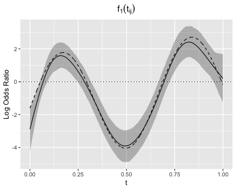
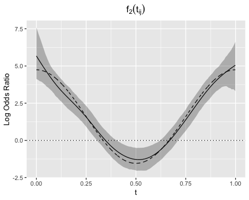
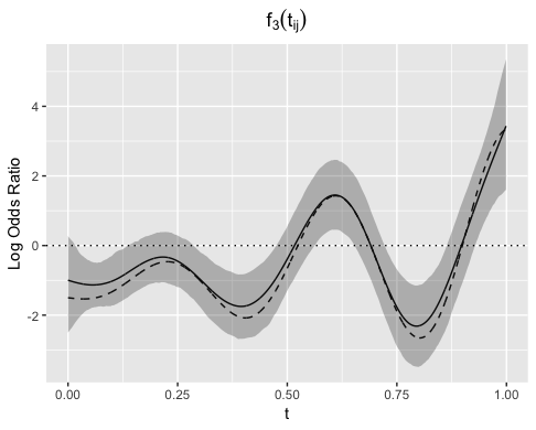
Table 4 reports results for our proposed method with SDP priors (PGBVSDP), our proposed method without SDP priors (PGBVS), peNMIG, and our model with horseshoe priors (PGHS) in terms of average sensitivity, specificity, and MCC for fixed (fSENS, fSPEC, fMCC) and random (rSENS, rSPEC, rMCC) effects across the replicate data sets with standard errors in parentheses. Additionally for the PGBVSDP model, we provide clustering performance results for fixed (fCLUST) and random effects (rCLUST). Since each of the random effects were simulated similarly, clusterings were compared to a single cluster for the non-zero terms. Overall, the methods had relatively similar results for fixed effects, with PGBVS and PGHS performing the best in terms of sensitivity (1.00 and 1.00) and MCC (0.96 and 0.99), respectively. Our method with SDP priors, PGBVSDP, obtained the highest specificity for fixed effects overall. Given that the maximum possible values fCLUST and rCLUST could take on were 3.4 and 2.7, respectively, we found fairly strong clustering performance for both fixed (0.39) and random (0.92) effects with PGBVSDP. We observed more variability in the selection of random effects across models. Random effect selection sensitivity was significantly lower compared to the fixed effects for all of the models. In terms of specificity (1-false positive rate) for random effects, our methods, regardless of prior formulation, dramatically outperformed peNMIG, with PGBVS obtaining the highest specificity overall (0.96). However, PGBVSDP and PGBVS had lower sensitivity with respect to random effects compared to PGHS. While PGHS performed well separating active from inactive random effects, recall that the truth was used to select the optimal selection threshold. The improved performance of PGBVS, PGBVSDP, and PGHS in terms of variable selection was achieved in considerably less computation time compared to peNMIG. Our core method was able to run 7,500 iterations in a fifth of the time compared to peNMIG, accessed via Scheipl 2011. Using the SDP priors, which requires additional updates for clustering the regression coefficients, we observed a two-fold increase in computation time for PGBVSDP compared to PGBVS. However on average, the PGBVSDP approach still achieved about a reduction in computation time compared to peNMIG. It is important to note that for comparison, all algorithms were run in series, even though the R package spikeSlabGAM (Scheipl 2011) provides functionality to run multiple chains in parallel.
| PGBVSDP | PGBVS | peNMIG | PGHS | ||||
|---|---|---|---|---|---|---|---|
| fSENS | 0.96 (0.09) | 1.00 (0.02) | 0.93 (0.11) | 1.00 (0.00) | |||
| fSPEC | 0.99 (0.02) | 0.98 (0.02) | 0.94 (0.04) | 0.96 (0.01) | |||
| fMCC | 0.94 (0.08) | 0.96 (0.05) | 0.83 (0.10) | 0.99 (0.02) | |||
| fCLUST | 0.39 (0.21) | - | - | - | |||
| rSENS | 0.76 (0.21) | 0.62 (0.25) | 0.46 (0.23) | 0.86 (0.24) | |||
| rSPEC | 0.88 (0.10) | 0.96 (0.05) | 0.64 (0.16) | 0.90 (0.11) | |||
| rMCC | 0.63 (0.26) | 0.64 (0.23) | 0.11 (0.33) | 0.76 (0.21) | |||
| rCLUST | 0.92 (0.50) | - | - | - | |||
| Time (s) | 4658 (271) | 2235 (46) | 10720 (1116) | 3076 (74) |
5 Sensitivity Analysis
To assess the model’s sensitivity to hyperparameter settings, we set each of the hyperparameters to default values and then evaluated the effect of manipulating each term on selection and clustering performance. For the default parameterization, we set the hyperparameters for the prior inclusion indicators and to . The default values for the variance of the normal distribution for the slab of and as well as the base distribution for were each fixed at . Additionally, the mean and variance for the random effect terms’ proposal and prior distributions were set to and , respectively. The hyperparameters for the concentration parameters, and . Lastly, we assumed . We ran our MCMC algorithm on the 50 replicated data sets generated in the simulation study, using 7,500 iterations, treating the first 3,750 iterations as burn-in and thinning to every iteration for the SDP model.
Results of the sensitivity analysis are reported in Table 5. As expected, we found that the sensitivity (specificity) increased (decreased) as the prior probability of inclusion for the fixed and random effects increased. The model did not seem sensitive to the variance assumed for the normal and folded normal priors assigned to the fixed and random effect slab distributions, respectively. Similarly, we found comparable results in terms of sensitivity and specificity for different values of the concentration parameters’ hyperparameters. In terms of clustering, we saw marginally better variation of information measures with larger concentration parameter hyperparameters. However across simulations runs, we observed relatively high standard errors in terms of the variation of information measures. To assess potential sensitivity to the order of random effects in our simulations, we re-ran the simulation study with a random permutation of the columns of . Similar to the case study, we found no evidence of sensitivity to random effect ordering with our model as the results were almost identical to those presented in Table 4 with PGBVSDP (rSENS = 0.76 (0.20), rSPEC = 0.87 (0.09), rMCC = 0.62 (0.20), rCLUST = 0.94 (0.42)).
| , | |||||
| fSENS | 0.92 (0.13) | 0.97 (0.08) | 0.94 (0.12) | ||
| fSPEC | 0.99 (0.02) | 0.99 (0.02) | 0.99 (0.02) | ||
| fMCC | 0.93 (0.10) | 0.96 (0.07) | 0.94 (0.09) | ||
| fCLUST | 0.45 (0.30) | 0.35 (0.20) | 0.45 (0.25) | ||
| rSENS | 0.50 (0.20) | 0.79 (0.20) | 0.54 (0.28) | ||
| rSPEC | 0.87 (0.09) | 0.88 (0.08) | 0.85 (0.10) | ||
| rMCC | 0.40 (0.26) | 0.66 (0.23) | 0.41 (0.29) | ||
| rCLUST | 1.30 (0.36) | 0.91 (0.44) | 1.25 (0.50) | ||
| , | |||||
| fSENS | 0.99 (0.03) | 0.96 (0.07) | 0.94 (0.11) | ||
| fSPEC | 0.96 (0.03) | 0.99 (0.02) | 0.99 (0.02) | ||
| fMCC | 0.91 (0.06) | 0.95 (0.07) | 0.93 (0.11) | ||
| fCLUST | 0.40 (0.20) | 0.39 (0.23) | 0.41 (0.24) | ||
| rSENS | 0.85 (0.20) | 0.78 (0.20) | 0.74 (0.23) | ||
| rSPEC | 0.84 (0.10) | 0.89 (0.10) | 0.86 (0.10) | ||
| rMCC | 0.66 (0.19) | 0.67 (0.25) | 0.60 (0.27) | ||
| rCLUST | 0.84 (0.49) | 0.89 (0.47) | 0.97 (0.49) |
6 Conclusions
In this paper, we have investigated intensive longitudinal data, collected in a novel, smartphone-based smoking cessation study to better understand the relation between potential risk factors and smoking behaviors in the critical moments surrounding a quit attempt, using a semiparametric Bayesian time-varying effect modeling framework. Unlike standard TVEMs, our approach deconstructs the structure of the relations between risk factors and smoking behaviors over time, which aids in formulating hypotheses regarding dynamic relations between risk factors and smoking in the critical moments around a quit attempt. By performing variable selection on random effects, the approach delivers additional insights on how relations vary over time as well as how they vary across individuals. Furthermore, the use of non- and semiparametric prior constructions allows simultaneous variable selection for fixed and random effects while learning latent clusters of regression coefficients. As such, our model is designed to discover various forms of latent structures within the data without requiring strict model assumptions or burdensome tuning procedures. Results from our analysis have confirmed previously identified temporal relations between smoking behaviors and urge to smoke, cigarette availability, and negative affect. They have also identified subject-specific heterogeneity in the effects of urge to smoke, cigarette availability, and motivation to quit. Additionally, we have found that subjects differed in how they responded to the SmartT treatment (compared to usual care), interacting with a smoker, and being bored over time. This has practical relevance as researchers can use this information to design adaptive interventions that prioritize targeting risk factors based on their relative strength of association at a given moment. They also reinforce the importance of designing dynamic intervention strategies that are adaptive to subjects’ current risk profiles.
Throughout this work, we have demonstrated how our method is well-suited to aide the development and evaluation of future JITAI strategies targeting smoking cessation using mHealth data. The existing SmartT algorithm delivers treatment based on the presence of six lapse triggers, which are weighted based on their relative importance in predicting risk of lapse (Businelle et al. 2016). The results of this study allow for a more dynamic algorithm that takes into account not only the time-varying relationships between psychosocial and environmental variables and smoking lapse, but the different ways in which individuals experience a quit attempt. For example, the results suggest that providing momentary support to cope with urge to smoke and negative affect may be more useful if delivered in the early stages of a quit attempt, but become less important by week 4 post-quit. However, messages that address cigarette availability, alcohol consumption, and motivation to quit smoking may be a more important focus for the entire quit attempt. Although the findings for this small sample may not be generalizable to larger, more diverse populations, these methods are the next step in developing a personalized smoking risk algorithm that can inform highly specific, individualized treatment to each smoker.
It is important to note that selection of a risk factor by our proposed method (or any variable selection technique), does not imply clinical significance. Notably, the point-wise credible intervals often contained odds ratios of one and most risk factors were only influential for brief moments throughout the study period. While these results highlight the importance of understanding risk factors’ dynamic relations with smoking to design tailored intervention strategies, we recommend using our method for hypothesis generation in practice and conducting confirmatory studies before generalizing results.
Compliance rates for EMA studies typically range between 70% and 90%, with a recommended threshold of 80% (Jones, Xu and Grunwald 2006). In our case study, the compliance rate was 84%. Additionally, 97.3% of all assessments were completed once initiated, and subjects were unable to skip questions within an assessment. Since subjects were assessed multiple times per day, nonresponse was attributed more to situational context (e.g., driving) than smoking status. Thus for this study, we found the missing completely at random assumption for missing observations justified. However, future studies may consider the development of advanced analytical methods for EMA data sets that can handle different types of missingness assumptions and other potential biases, such as social desirability bias.
In this analysis, we focus on time-varying effects due to their recent popularity in smoking behavior research Tan et al. 2012; Shiyko et al. 2012; Vasilenko et al. 2014; Koslovsky et al. 2017; Lanza et al. 2013; Shiyko et al. 2014. A promising alternative for investigating the complexity of smoking behaviors around a quit attempt is the varying index coefficient model, which allows a covariate’s effect to vary as a function of multiple other variables (Ma and Song 2015). By incorporating variable selection priors, researchers could identify which variables are responsible for modifying a covariate’s effect. Oftentimes behavioral researchers are interested in exploring other forms of latent structure, such as clusters of individuals who respond similarly to treatments or have similar risk profiles over time. Taking advantage of the flexibility and efficiency of our approach, future work could extend our core model to address these research questions by recasting it into a mixture modeling framework. In addition, while we have developed our method for binary outcomes due to their prevalence in smoking behavior research studies, our approach is easily adaptable to other data structures found within and outside of smoking behavior research, such as time to event data (Sha, Tadesse and Vannucci 2006) and continuous outcomes. While our method borrows information across regression coefficients, we avoided imposing structure among covariates via heredity constraints, which restrict the model space for higher order terms depending on the inclusion status of the lower order terms that comprise them. Researchers interested in extending our approach to accommodate these, and other forms of, hierarchical constraints may adjust the prior probabilities of inclusion (Chipman 1996). Lastly, while we were hesitant to present variable selection results for PGHS, due to the limited understanding of global-local priors for non-Gaussian distributions, this showed good results in simulations. Furthermore, when applied to the case study data, we obtained promising predictive performance (i.e., ) that warrant future investigation of its theoretical properties.
Acknowledgements
Matthew Koslovsky is supported by NSF via the Research Training Group award DMS-1547433.
Supplementary Material
R-package for PGBVS:
R-package PGBVS contains code to perform the methods described in the article. The package also contains functionality for reproducing the data used in the sensitivity and simulation studies and for posterior inference. The R package is located at https://github.com/mkoslovsky/PGBVS.
Supplementary Information:
This file contains a description of the full joint distribution of our model with a graphical representation, a detailed description of our proposed MCMC algorithm with and without SDP priors, and derivations for the prior marginal likelihood used to sample latent cluster assignments. Additionally, we include details of the goodness-of-fit analysis for the case study.
References
- Barbieri et al. (2004) [author] Barbieri, Maria MaddalenaM. M., Berger, James OJ. O. et al. (2004). Optimal predictive model selection. The Annals of Statistics 32 870–897.
- Berardi et al. (2018) [author] Berardi, VincentV., Carretero-González, RicardoR., Bellettiere, JohnJ., Adams, Marc AM. A., Hughes, SuzanneS. and Hovell, MelbourneM. (2018). A Markov approach for increasing precision in the assessment of data-intensive behavioral interventions. Journal of Biomedical Informatics 85 93–105.
- Bhadra et al. (2019) [author] Bhadra, AnindyaA., Datta, JyotishkaJ., Polson, Nicholas GN. G., Willard, BrandonB. et al. (2019). Lasso meets horseshoe: A survey. Statistical Science 34 405–427.
- Bolman et al. (2018) [author] Bolman, CatherineC., Verboon, PeterP., Thewissen, VivianneV., Boonen, VivianeV., Soons, KarinK. and Jacobs, NeleN. (2018). Predicting smoking lapses in the first week of quitting: an ecological momentary assessment study. Journal of Addiction Medicine 12 65.
- Brook et al. (2008) [author] Brook, David WD. W., Brook, Judith SJ. S., Zhang, ChenshuC., Whiteman, MartinM., Cohen, PatriciaP. and Finch, Stephen JS. J. (2008). Developmental trajectories of cigarette smoking from adolescence to the early thirties: personality and behavioral risk factors. Nicotine & Tobacco Research 10 1283–1291.
- Brown, Vannucci and Fearn (1998) [author] Brown, Philip JP. J., Vannucci, MarinaM. and Fearn, TomT. (1998). Multivariate Bayesian variable selection and prediction. Journal of the Royal Statistical Society: Series B (Statistical Methodology) 60 627–641.
- Businelle et al. (2014) [author] Businelle, Michael SM. S., Ma, PingP., Kendzor, Darla ED. E., Reitzel, Lorraine RL. R., Chen, MinxingM., Lam, Cho YC. Y., Bernstein, IraI. and Wetter, David WD. W. (2014). Predicting quit attempts among homeless smokers seeking cessation treatment: an ecological momentary assessment study. Nicotine & Tobacco Research 16 1371-1378.
- Businelle et al. (2016) [author] Businelle, Michael SM. S., Ma, PingP., Kendzor, Darla ED. E., Frank, Summer GS. G., Vidrine, Damon JD. J. and Wetter, David WD. W. (2016). An ecological momentary intervention for smoking cessation: evaluation of feasibility and effectiveness. Journal of Medical Internet Research 18 e321.
- Cai and Bandyopadhyay (2017) [author] Cai, BoB. and Bandyopadhyay, DipankarD. (2017). Bayesian semiparametric variable selection with applications to periodontal data. Statistics in Medicine 36 2251–2264.
- Canale et al. (2017) [author] Canale, AntonioA., Lijoi, AntonioA., Nipoti, BernardoB. and Prünster, IgorI. (2017). On the Pitman–Yor process with spike and slab base measure. Biometrika 104 681–697.
- Carvalho, Polson and Scott (2009) Carvalho, C. M., Polson, N. G. and Scott, J. G. (2009). Handling sparsity via the horseshoe. In Artificial Intelligence and Statistics 73–80.
- Chen and Dunson (2003) [author] Chen, ZhenZ. and Dunson, David BD. B. (2003). Random effects selection in linear mixed models. Biometrics 59 762–769.
- Cheng et al. (2010) [author] Cheng, JingJ., Edwards, Lloyd JL. J., Maldonado-Molina, Mildred MM. M., Komro, Kelli AK. A. and Muller, Keith EK. E. (2010). Real longitudinal data analysis for real people: building a good enough mixed model. Statistics in Medicine 29 504–520.
- Chipman (1996) [author] Chipman, HughH. (1996). Bayesian variable selection with related predictors. The Canadian Journal of Statistics 17-36.
- Cursio, Mermelstein and Hedeker (2019) [author] Cursio, John FJ. F., Mermelstein, Robin JR. J. and Hedeker, DonaldD. (2019). Latent trait shared-parameter mixed models for missing ecological momentary assessment data. Statistics in Medicine 38 660–673.
- Dahl and Muller (2017) [author] Dahl, D. B.D. B. and Muller, P.P. (2017). sdols: Summarizing Distributions of Latent Structures. R package version 1.4. 591.
- de Haan-Rietdijk et al. (2017) [author] de Haan-Rietdijk, SS., Kuppens, PeterP., Bergeman, Cindy SC. S., Sheeber, LBL., Allen, NBN. and Hamaker, ELE. (2017). On the use of mixed Markov models for intensive longitudinal data. Multivariate Behavioral Research 52 747–767.
- Dunson, Herring and Engel (2008) [author] Dunson, David BD. B., Herring, Amy HA. H. and Engel, Stephanie MS. M. (2008). Bayesian selection and clustering of polymorphisms in functionally related genes. Journal of the American Statistical Association 103 534–546.
- Dziak et al. (2015) [author] Dziak, John JJ. J., Li, RunzeR., Tan, XianmingX., Shiffman, SaulS. and Shiyko, Mariya PM. P. (2015). Modeling intensive longitudinal data with mixtures of nonparametric trajectories and time-varying effects. Psychological Methods 20 444.
- Escobar and West (1995) [author] Escobar, Michael DM. D. and West, MikeM. (1995). Bayesian density estimation and inference using mixtures. Journal of the American Statistical Association 90 577–588.
- Fitzmaurice, Laird and Ware (2012) [author] Fitzmaurice, Garrett MG. M., Laird, Nan MN. M. and Ware, James HJ. H. (2012). Applied Longitudinal Analysis 998. John Wiley & Sons.
- Geiser et al. (2013) [author] Geiser, ChristianC., Bishop, JacobJ., Lockhart, GingerG., Shiffman, SaulS. and Grenard, Jerry LJ. L. (2013). Analyzing latent state-trait and multiple-indicator latent growth curve models as multilevel structural equation models. Frontiers in Psychology 4 975.
- Gelfand (1996) [author] Gelfand, Alan EA. E. (1996). Model determination using sampling-based methods. Markov chain Monte Carlo in practice 145–161.
- Gelman and Rubin (1992) [author] Gelman, AndrewA. and Rubin, Donald BD. B. (1992). Inference from iterative simulation using multiple sequences. Statistical science 7 457–472.
- Gelman et al. (2000) [author] Gelman, AndrewA., Goegebeur, YuriY., Tuerlinckx, FrancisF. and Van Mechelen, IvenI. (2000). Diagnostic checks for discrete data regression models using posterior predictive simulations. Journal of the Royal Statistical Society: Series C (Applied Statistics) 49 247–268.
- George and McCulloch (1993) [author] George, Edward IE. I. and McCulloch, Robert ER. E. (1993). Variable selection via Gibbs sampling. Journal of the American Statistical Association 88 881–889.
- George and McCulloch (1997) [author] George, Edward IE. I. and McCulloch, Robert ER. E. (1997). Approaches for Bayesian variable selection. Statistica Sinica 339–373.
- Hastie and Tibshirani (1993) [author] Hastie, TrevorT. and Tibshirani, RobertR. (1993). Varying-coefficient models. Journal of the Royal Statistical Society: Series B (Methodological) 55 757–779.
- Heron and Smyth (2010) [author] Heron, Kristin EK. E. and Smyth, Joshua MJ. M. (2010). Ecological momentary interventions: Incorporating mobile technology into psychosocial and health behaviour treatments. British Journal of Health Psychology 15 1–39.
- Hui, Müller and Welsh (2017) [author] Hui, Francis KCF. K., Müller, SamuelS. and Welsh, AHA. (2017). Hierarchical selection of fixed and random effects in generalized linear mixed models. Statistica Sinica 501–518.
- Ishwaran et al. (2005) [author] Ishwaran, HemantH., Rao, J SunilJ. S. et al. (2005). Spike and slab variable selection: frequentist and Bayesian strategies. The Annals of Statistics 33 730–773.
- Jones, Xu and Grunwald (2006) [author] Jones, Richard HR. H., Xu, StanleyS. and Grunwald, Gary KG. K. (2006). Continuous time Markov models for binary longitudinal data. Biometrical Journal 48 411–419.
- Kim, Dahl and Vannucci (2009) [author] Kim, SinaeS., Dahl, David BD. B. and Vannucci, MarinaM. (2009). Spiked Dirichlet process prior for Bayesian multiple hypothesis testing in random effects models. Bayesian Analysis (Online) 4 707.
- Kinney and Dunson (2007) [author] Kinney, Satkartar KS. K. and Dunson, David BD. B. (2007). Fixed and random effects selection in linear and logistic models. Biometrics 63 690–698.
- Klasnja et al. (2015) [author] Klasnja, PredragP., Hekler, Eric BE. B., Shiffman, SaulS., Boruvka, AudreyA., Almirall, DanielD., Tewari, AmbujA. and Murphy, Susan AS. A. (2015). Microrandomized trials: An experimental design for developing just-in-time adaptive interventions. Health Psychology 34 1220.
- Koslovsky et al. (2017) [author] Koslovsky, Matthew DM. D., Hébert, Emily TE. T., Swartz, Michael DM. D., Chan, WenyawW., Leon-Novelo, LuisL., Wilkinson, Anna VA. V., Kendzor, Darla ED. E. and Businelle, Michael SM. S. (2017). The time-varying relations between risk factors and smoking before and after a quit attempt. Nicotine & Tobacco Research.
- Koslovsky et al. (2018) [author] Koslovsky, Matthew DM. D., Swartz, Michael DM. D., Chan, WenyawW., Leon-Novelo, LuisL., Wilkinson, Anna VA. V., Kendzor, Darla ED. E. and Businelle, Michael SM. S. (2018). Bayesian variable selection for multistate Markov models with interval-censored data in an ecological momentary assessment study of smoking cessation. Biometrics 74 636–644.
- Kürüm et al. (2016) [author] Kürüm, EsraE., Li, RunzeR., Shiffman, SaulS. and Yao, WeixinW. (2016). Time-varying coefficient models for joint modeling binary and continuous outcomes in longitudinal data. Statistica Sinica 26 979.
- Lang and Brezger (2004) [author] Lang, StefanS. and Brezger, AndreasA. (2004). Bayesian P-splines. Journal of Computational and Graphical Statistics 13 183–212.
- Lanza et al. (2013) [author] Lanza, Stephanie TS. T., Vasilenko, Sara AS. A., Liu, XiaoyuX., Li, RunzeR. and Piper, Megan EM. E. (2013). Advancing the understanding of craving during smoking cessation attempts: A demonstration of the time-varying effect model. Nicotine & Tobacco Research.
- Li, Müller and Lin (2011) [author] Li, YishengY., Müller, PeterP. and Lin, XihongX. (2011). Center-adjusted inference for a nonparametric Bayesian random effect distribution. Statistica Sinica 21.
- Luckett et al. (2019) [author] Luckett, Daniel JD. J., Laber, Eric BE. B., Kahkoska, Anna RA. R., Maahs, David MD. M., Mayer-Davis, ElizabethE. and Kosorok, Michael RM. R. (2019). Estimating dynamic treatment regimes in mobile health using V-learning. Journal of the American Statistical Association 1–39.
- Ma and Song (2015) [author] Ma, ShujieS. and Song, Peter X-KP. X.-K. (2015). Varying index coefficient models. Journal of the American Statistical Association 110 341–356.
- Mason et al. (2015) [author] Mason, MichaelM., Mennis, JeremyJ., Way, ThomasT., Lanza, StephanieS., Russell, MichaelM. and Zaharakis, NikolaN. (2015). Time-varying effects of a text-based smoking cessation intervention for urban adolescents. Drug and Alcohol Dependence 157 99–105.
- McCarthy et al. (2016) [author] McCarthy, Danielle ED. E., Ebssa, LemmaL., Witkiewitz, KatieK. and Shiffman, SaulS. (2016). Repeated measures latent class analysis of daily smoking in three smoking cessation studies. Drug and Alcohol Dependence 165 132–142.
- McClure et al. (2016) [author] McClure, Jennifer BJ. B., Anderson, Melissa LM. L., Bradley, KatharineK., An, Lawrence CL. C. and Catz, Sheryl LS. L. (2016). Evaluating an adaptive and interactive mHealth smoking cessation and medication adherence program: a randomized pilot feasibility study. JMIR mHealth and uHealth 4 e94.
- Meilă (2003) [author] Meilă, MarinaM. (2003). Comparing clusterings by the variation of information. In Learning Theory and Kernel Machines 173–187. Springer.
- Minami et al. (2014) [author] Minami, HarukaH., Yeh, Vivian MV. M., Bold, Krysten WK. W., Chapman, Gretchen BG. B. and McCarthy, Danielle ED. E. (2014). Relations among affect, abstinence motivation and confidence, and daily smoking lapse risk. Psychology of Addictive Behaviors 28 376.
- Müller, Quintana and Rosner (2007) [author] Müller, PeterP., Quintana, Fernando AF. A. and Rosner, Gary LG. L. (2007). Semiparametric Bayesian inference for multilevel repeated measurement data. Biometrics 63 280–289.
- Müller et al. (2013) [author] Müller, SamuelS., Scealy, Janice LJ. L., Welsh, Alan HA. H. et al. (2013). Model selection in linear mixed models. Statistical Science 28 135–167.
- Nahum-Shani et al. (2017) [author] Nahum-Shani, InbalI., Smith, Shawna NS. N., Spring, Bonnie JB. J., Collins, Linda ML. M., Witkiewitz, KatieK., Tewari, AmbujA. and Murphy, Susan AS. A. (2017). Just-in-time adaptive interventions (JITAIs) in mobile health: Key components and design principles for ongoing health behavior support. Annals of Behavioral Medicine 52 446–462.
- Naughton et al. (2016) [author] Naughton, FelixF., Hopewell, SarahS., Lathia, NealN., Schalbroeck, RikR., Brown, ChloëC., Mascolo, CeciliaC., McEwen, AndyA. and Sutton, StephenS. (2016). A context-sensing mobile phone app (Q sense) for smoking cessation: a mixed-methods study. JMIR mHealth and uHealth 4 e106.
- Neal (2000) [author] Neal, Radford MR. M. (2000). Markov chain sampling methods for Dirichlet process mixture models. Journal of Computational and Graphical Statistics 9 249–265.
- Newton et al. (2004) [author] Newton, Michael AM. A., Noueiry, AmineA., Sarkar, DeepayanD. and Ahlquist, PaulP. (2004). Detecting differential gene expression with a semiparametric hierarchical mixture method. Biostatistics 5 155–176.
- Piasecki et al. (2002) [author] Piasecki, Thomas MT. M., Fiore, Michael CM. C., McCarthy, Danielle ED. E. and Baker, Timothy BT. B. (2002). Have we lost our way? The need for dynamic formulations of smoking relapse proneness. Addiction 97 1093-1108.
- Piasecki et al. (2003) [author] Piasecki, Thomas MT. M., Jorenby, Douglas ED. E., Smith, Stevens SS. S., Fiore, Michael CM. C. and Baker, Timothy BT. B. (2003). Smoking withdrawal dynamics:II. Improved tests of withdrawal-relapse relations. Journal of Abnormal Psychology 112 14.
- Piasecki et al. (2013) [author] Piasecki, Thomas MT. M., Trela, Constantine JC. J., Hedeker, DonaldD. and Mermelstein, Robin JR. J. (2013). Smoking antecedents: Separating between-and within-person effects of tobacco dependence in a multiwave ecological momentary assessment investigation of adolescent smoking. Nicotine & Tobacco Research 16 S119–S126.
- Polson and Scott (2010) [author] Polson, Nicholas GN. G. and Scott, James GJ. G. (2010). Shrink globally, act locally: Sparse Bayesian regularization and prediction. Bayesian statistics 9 105.
- Polson, Scott and Windle (2013) [author] Polson, Nicholas GN. G., Scott, James GJ. G. and Windle, JesseJ. (2013). Bayesian inference for logistic models using Pólya–Gamma latent variables. Journal of the American Statistical Association 108 1339–1349.
- Riley et al. (2011) [author] Riley, William TW. T., Rivera, Daniel ED. E., Atienza, Audie AA. A., Nilsen, WendyW., Allison, Susannah MS. M. and Mermelstein, RobinR. (2011). Health behavior models in the age of mobile interventions: Are our theories up to the task? Translational Behavioral Medicine 1 53–71.
- Rivera, Pew and Collins (2007) [author] Rivera, Daniel ED. E., Pew, Michael DM. D. and Collins, Linda ML. M. (2007). Using engineering control principles to inform the design of adaptive interventions: A conceptual introduction. Drug and Alcohol Dependence 88 S31–S40.
- Savitsky and Vannucci (2010) [author] Savitsky, TerranceT. and Vannucci, MarinaM. (2010). Spiked Dirichlet process priors for Gaussian process models. Journal of Probability and Statistics 2010.
- Savitsky, Vannucci and Sha (2011) [author] Savitsky, TerranceT., Vannucci, MarinaM. and Sha, NaijunN. (2011). Variable selection for nonparametric Gaussian process priors: Models and computational strategies. Statistical Science: A review Journal of the Institute of Mathematical Statistics 26 130-149.
- Scheipl (2011) [author] Scheipl, FabianF. (2011). spikeSlabGAM: Bayesian variable selection, model choice and regularization for generalized additive mixed models in R. arXiv preprint arXiv:1105.5253.
- Scheipl, Fahrmeir and Kneib (2012) [author] Scheipl, FabianF., Fahrmeir, LudwigL. and Kneib, ThomasT. (2012). Spike-and-slab priors for function selection in structured additive regression models. Journal of the American Statistical Association 107 1518–1532.
- Selya et al. (2015) [author] Selya, Arielle SA. S., Updegrove, NicoleN., Rose, Jennifer SJ. S., Dierker, LisaL., Tan, XianmingX., Hedeker, DonaldD., Li, RunzeR. and Mermelstein, Robin JR. J. (2015). Nicotine-dependence-varying effects of smoking events on momentary mood changes among adolescents. Addictive Behaviors 41 65–71.
- Sha, Tadesse and Vannucci (2006) [author] Sha, NaijunN., Tadesse, Mahlet GM. G. and Vannucci, MarinaM. (2006). Bayesian variable selection for the analysis of microarray data with censored outcomes. Bioinformatics 22 2262–2268.
- Shiffman (2013) [author] Shiffman, SaulS. (2013). Conceptualizing analyses of ecological momentary assessment data. Nicotine & Tobacco Research 16 S76–S87.
- Shiffman et al. (1996) [author] Shiffman, SaulS., Paty, Jean AJ. A., Gnys, MaryannM., Kassel, Jon AJ. A. and Hickcox, MaryM. (1996). First lapses to smoking: within-subjects analysis of real-time reports. Journal of Consulting and Clinical Psychology 64 366.
- Shiffman et al. (2000) [author] Shiffman, SaulS., Balabanis, Mark HM. H., Paty, Jean AJ. A., Engberg, JohnJ., Gwaltney, Chad JC. J., Liu, Kenneth SK. S., Gnys, MaryannM., Hickcox, MaryM. and Paton, Stephanie MS. M. (2000). Dynamic effects of self-efficacy on smoking lapse and relapse. Health Psychology 19 315.
- Shiffman et al. (2002) [author] Shiffman, SaulS., Gwaltney, Chad JC. J., Balabanis, Mark HM. H., Liu, Kenneth SK. S., Paty, Jean AJ. A., Kassel, Jon DJ. D., Hickcox, MaryM. and Gnys, MaryannM. (2002). Immediate antecedents of cigarette smoking: an analysis from ecological momentary assessment. Journal of Abnormal Psychology 111 531.
- Shiyko et al. (2012) [author] Shiyko, Mariya PM. P., Lanza, Stephanie TS. T., Tan, XianmingX., Li, RunzeR. and Shiffman, SaulS. (2012). Using the time-varying effect model (TVEM) to examine dynamic associations between negative affect and self confidence on smoking urges: Differences between successful quitters and relapsers. Prevention Science 13 288-299.
- Shiyko et al. (2014) [author] Shiyko, MariyaM., Naab, PamelaP., Shiffman, SaulS. and Li, RunzeR. (2014). Modeling Complexity of eMa Data: time-varying lagged effects of negative affect on smoking Urges for subgroups of nicotine addiction. Nicotine & Tobacco Research 16 S144–S150.
- Tan et al. (2012) [author] Tan, XianmingX., Shiyko, Mariya PM. P., Li, RunzeR., Li, YuelinY. and Dierker, LisaL. (2012). A time-varying effect model for intensive longitudinal data. Psychological Methods 17 61.
- Timms et al. (2013) [author] Timms, Kevin PK. P., Rivera, Daniel ED. E., Collins, Linda ML. M. and Piper, Megan EM. E. (2013). A dynamical systems approach to understanding self-regulation in smoking cessation behavior change. Nicotine & Tobacco Research 16 S159–S168.
- Trail et al. (2014) [author] Trail, Jessica BJ. B., Collins, Linda ML. M., Rivera, Daniel ED. E., Li, RunzeR., Piper, Megan EM. E. and Baker, Timothy BT. B. (2014). Functional data analysis for dynamical system identification of behavioral processes. Psychological Methods 19 175.
- Van Erp, Oberski and Mulder (2019) [author] Van Erp, SaraS., Oberski, Daniel LD. L. and Mulder, JorisJ. (2019). Shrinkage priors for Bayesian penalized regression. Journal of Mathematical Psychology 89 31–50.
- Vasilenko et al. (2014) [author] Vasilenko, Sara AS. A., Piper, Megan EM. E., Lanza, Stephanie TS. T., Liu, XiaoyuX., Yang, JingyunJ. and Li, RunzeR. (2014). Time-varying processes involved in smoking lapse in a randomized trial of smoking cessation therapies. Nicotine & Tobacco Research 16 S135–S143.
- Vehtari, Gelman and Gabry (2016) [author] Vehtari, AkiA., Gelman, AndrewA. and Gabry, JonahJ. (2016). loo: Efficient leave-one-out cross-validation and WAIC for Bayesian models. R package version 0.1 6.
- Vehtari, Gelman and Gabry (2017) [author] Vehtari, AkiA., Gelman, AndrewA. and Gabry, JonahJ. (2017). Practical Bayesian model evaluation using leave-one-out cross-validation and WAIC. Statistics and Computing 27 1413–1432.
- Wade et al. (2018) [author] Wade, SaraS., Ghahramani, ZoubinZ. et al. (2018). Bayesian cluster analysis: Point estimation and credible balls (with discussion). Bayesian Analysis 13 559–626.
- Walls and Schafer (2005) [author] Walls, Theodore AT. A. and Schafer, Joseph LJ. L. (2005). Models for intensive longitudinal data. Oxford University Press.
- Yang (2012) [author] Yang, MinganM. (2012). Bayesian variable selection for logistic mixed model with nonparametric random effects. Computational Statistics & Data Analysis 56 2663–2674.