2022
Stroke is known as a major global health problem, and for stroke survivors it is key to monitor the recovery levels. However, traditional stroke rehabilitation assessment methods (such as the popular clinical assessment) can be subjective and expensive, and it is also less convenient for patients to visit clinics in a high frequency. To address this issue, in this work based on wearable sensing and machine learning techniques, we \colorblack develop an automated system that can predict the assessment score in an objective manner. With wrist-worn sensors, accelerometer data \colorblack is collected from 59 stroke survivors in free-living environments for a duration of 8 weeks, and we \colorblack map the week-wise accelerometer data (3 days per week) to the assessment score by developing signal processing and predictive model pipeline. To achieve this, we \colorblack propose two types of new features, which can encode the rehabilitation information from both paralysed and non-paralysed sides while suppressing the high-level noises such as irrelevant daily activities. Based on the proposed features, we further \colorblack develop the longitudinal mixed-effects model with Gaussian process prior (LMGP), which can model the random effects caused by different subjects and time slots (during the 8 weeks). Comprehensive experiments \colorblack are conducted to evaluate our system on both acute and chronic patients, and \colorblack the promising results suggest its effectiveness.
Designing Compact Features for Remote Stroke Rehabilitation Monitoring using Wearable Accelerometers
keywords
wrist-worn accelerometer sensor, stroke rehabilitation, CAHAI score, regression model1 Introduction
It is widely known that stroke is a worldwide health problem causing disability and death Donnan:2008, and it occurs when a blood clot cuts off oxygen supply to a region of the brain. Hemiparesis is a very common symptom of post-stroke that is the fractional or intact paralysis of one side of the body, i.e., the opposite side to where the blood clot \colorblack occurs, and it results in difficulties in performing activities, e.g., \colorblack with reduced arm movement. Patients can recover some of their capabilities with intense therapeutic input, so it is important to assess their recovery levels in time. There are many approaches to assess patients’ recovery levels including brain imaging BrainImaging_2005, questionnaire-based Questionaires_2007, and lab-based clinical assessment CAHAI_2005.
The brain imaging technique, is deemed as one of the most reliable approach, which can provide the information of brain hemodynamics BrainImaging_2005. However, this approach requires special equipment and is very expensive in cost. Questionnaire-based approaches investigate the functional ability during a period using questionnaires, and it can be categorised into two types: patient-completed and caregiver-completed Questionaires_2007. Although it is much cheaper than brain imaging approaches, it may contain high-level of bias. For instance, patients may not remember their daily activities (i.e.,recall bias); the caregivers may not be able to observe the patient all the time. These biases make questionnaire-based approaches less precise. Lab-based clinical assessment approaches CAHAI_2005Barreca:2005, on the other hand, provide an alternative solution. The patients’ upper limb functionality will be assessed by clinicians, e.g., by observing patients’ capabilities of finishing certain pre-defined activities CAHAI_2005. Compared with braining imaging or questionnaire-based approaches, the cost of lab-based clinical assessment approaches is reasonable with high accuracy. However, this assessment is normally taken in clinics/hospitals, which is not convenient for the patients, making continuous monitoring less feasible.
In this work, we aim to build an automated stroke rehabilitation assessment system using wearable sensing and machine learning techniques. Different from the aforementioned approaches, our system can measure the patients objectively and continuously in free-living environments. We \colorblack collect accelerometer data using wrist-worn accelerometer sensors, and \colorblack design compact features that can capture rehabilitation-related movements, before mapping these features to clinical assessment scores (i.e., the model training process). The trained model can be used to infer recovery-level for other unknown patients. In free living environments, there are different types of movements which may be related to different frequencies. For example, activities such as running or jumping may correspond to high-frequency signals, while sedentary or eating may be low-frequency signals. In this study, instead of recognising the daily activities explicitly, which is hard to achieve given limited annotation (e.g., without frame/sample-wise annotation), we \colorblack transform the raw accelerometer data to the frequency domain, where we design features that can encode the rehabilitation-related movements. Specifically, wavelet transform waveletbook \colorblack is used, and the wavelet coefficients can represent the particular frequency information at certain decomposition scales. In Preece:2009, Preece et al. \colorblack provide some commonly used wavelet features extracted from accelerometer data. However, to capture stroke rehabilitation-related activities, some domain knowledge should be taken into account to design better features. After stroke, patients have difficulties in moving one side (i.e., paralysed side) due to the brain injury, and data from paralysed side tends to describe more about the upper limb functional ability, than the non-paralysed side (i.e., normal side). However, such signals can be significantly affected by personal behaviours or irrelevant daily activities, and such noises should be suppressed before developing the predictive models. Various wavelet features were studied, and we \colorblack propose two new types of daily-activity-invariant features that can encode information from both paralysed/non-paralysed sides, before developing predictive models for stroke rehabilitation assessment. Specifically, in this work our contributions can be summarised as follows:
- •
Stroke-rehab-driven Features: We \colorblack propose two new types of compact wavelet-based features that can encode information from both paralysed and non-paralysed sides to represent upper limb functional abilities for stroke rehabilitation assessment. It can significantly suppress the influences of personal behaviours or irrelevant daily activities for data collected in the noisy free-living environment.
- •
Automated Assessment System: Based on the proposed stroke-rehab-driven features, we developed the automated system by using the longitudinal mixed-effects model with Gaussian process prior (LMGP). Various predictive models were studied, and we \colorblack find LMGP can model the random effects caused by the heterogeneity nature among subjects in a 8-week longitudinal study.
- •
Comprehensive Evaluation: Comprehensive experiments \colorblack are designed to study the effectiveness of our system. We comprehensively studied the feature subset on modelling the mixed-effects of LMGP. Compared with other approaches, the results \colorblack suggest the effectiveness of the proposed system on both acute and chronic patients.
.
2 Background and Related Work
As described in Sec.1, lab-based clinical assessment \colorblack is one of the most effective stroke rehabilitation assessment methods. In this section, we introduce the lab-based approach named Chedoke Arm and Hand Activity Inventory (CAHAI) scoring Barreca:2006b, based on which our automated system can be developed. Some sensing and machine learning techniques for automated health assessment are also \colorblack reviewed in this section.

2.1 Chedoke Arm and Hand Activity Inventory (CAHAI)
CAHAI scoring is a clinical assessment method for stroke rehabilitation, and it is a fully validated measure Barreca:2006b of upper limb functional ability with 9 tasks which are scored by using a 7-point quantitative scale. In the assessment, the patient will be asked to perform 9 tasks, including opening a jar of coffee, drawing a line with a ruler, calling 911, etc. and the clinician will score these behaviours based on patient’s performance at a scale from 1 (total assist weak) to 7 (complete independence i.e., timely, safely) Barreca:2006b. A task example ”call 911” is shown in Fig. 1. Thus the minimum and maximum summation scores are 7 and 63 respectively. A CAHAI score form can be found in Fig.12 in Appendix 5.2.
2.2 Automated Behaviour Assessment using Wearables
Recently, wearable sensing and machine learning (ML) techniques \colorblack are comprehensively studied for automated health assessment. Compared with the traditional assessment approaches (e.g., via self-reporting, clinical assessment, etc.) which are normally subjective and expensive, the automated systems may provide an objective, low-cost alternative, which can also be used for continuous monitoring/assessment. Some automated systems \colorblack are developed to assess the behaviours of diseases such as Parkinson’s disease PD_Rehman19 Nils_PD15, autism TP_autism, depression Little_depression2020; or to monitor the health status such as sleep Bing_sleep Yike_sleep, fatigue Yang_ISWC, Fatigue_IMU or recover-level from surgery Anna_IMU gait_surgery, etc.
After collecting behaviour or physiological signals (e.g., accelerometers, ECG, audio, etc.), assessment/monitoring models can be developed. For application with high interpretability requirement, feature engineering can be a crucial step. For example, with gait parameters extracted from IMU sensors (such as stride, velocity, etc.), one can build simple ML models (e.g., random forest) for Parkinson’s disease classification PD_Rehman19 or fatigue score regression Fatigue_IMU. Compared with the redundant IMU data, gait parameters are more compact and interpretable, making it suitable for clinical applications. However, designing interpretable/clinically-relevant features can be a time-consuming process, which may also require domain knowledge Bing_sleepFatigue_IMU PD_Rehman19Anna_IMU gait_surgery.
On the other hand, when interpretability is less required, deep learning can be an alternative approach, which can be directly applied to the raw signal Yike_sleep or engineered features Nils_PD15 Bing_sleep Yang_ISWC Little_depression2020 for (high-level) representation learning and classification/regression tasks. However, it normally requires adequate data annotation for better model generalisation.
2.3 Sensing Techniques for Automated Stroke Rehabilitation Monitoring
With the rapid development of the sensing/ML techniques, researchers also \colorblack start to apply various sensors for stroke rehabilitation monitoring. In Dolatabadi:2017, Kinect sensor \colorblack is used in a home-like environments to detect the key joints such that stroke patients’ behaviour can be assessed. In sensing_sEMG, a wireless surface Electromyography (sEMG) device \colorblack is used to monitor the muscle recruitment of the post-stroke patients to see the effect of orthotic intervention. In clinical environments, five wearable sensors \colorblack are placed on the trunk, upper and forearm of the two upper limbs to measure the reaching behaviours of the stroke survivors sensing_5sensors. To monitor motor functions of stroke patients during rehabilitation sessions at clinics, an ecosystem including a jack and a cube for hand grasping monitoring, as well as a smart watch for arm dynamic monitoring was designed sensing_ecosystem. These techniques can objectively assess/measure the behaviours of the stroke patients, yet they are either limited to clinical environments sensing_ecosystemsensing_5sensors sensing_sEMG or constrained environments (e.g., in front of a camera Dolatabadi:2017).
Most recently, wrist-worn sensors \colorblack are used for stroke rehabilitation monitoring for patients in free-living environment Shane_ISWC Tang_stroke. In each trial, 3-day accelerometer data \colorblack are collected from both wrists (with a trial-wise annotation, i.e., CAHAI score), and for both works Shane_ISWC Tang_stroke data analysis \colorblack is performed using the sliding window approach. To reduce the data redundancy of the raw data, PCA features \colorblack are extracted from each window Shane_ISWC Tang_stroke. Moreover, due to the lack of window-wise annotation, in Shane_ISWC pseudo label \colorblack is assigned to each window such that a random forest regressor can be trained, while in Tang_stroke Gaussian Mixture Models (GMM) clustering approach \colorblack is employed to learn the holistic trial-wise representation, before developing the regression model. Both methods Shane_ISWC Tang_stroke \colorblack suffer from the lack of annotation. In Shane_ISWC,pseudo labeling \colorblack is introduced, yet the trained model \colorblack is affected by the introduced label noise. In Tang_stroke, the application of GMM clustering (on the sliding windows) \colorblack makes it computationally expensive to large data, and the trained model \colorblack does not generalise well to unseen subjects.
In our work, by analysing the nature of the paralysed/non-paralysed sides, we design stroke-rehab-driven features which can directly encode the long accelerometer sequence (e.g., a trial with 3-day accelerometer data) into a very compact representation. The features are expected to emphasis the stroke-related behaviours while suppressing the irrelevant activities. Based on the proposed features, a predictive model that is adaptive to different subjects/time-slots can be developed using LMGP Shi:2012 for CAHAI score prediction.
3 Methodology
In this section, we \colorblack introduce our method from data collection, data pre-processing, feature design to predictive models. Our aim is to develop an automated model which can map the free-living 3-day accelerometer data into the CAHAI score. With the trained model, we can automatically infer the CAHAI score in an objective and continuous manner. To achieve this, we first \colorblack reduce the data redundancy via preprocessing and design compact and discriminant features. Given the proposed features, a longitudinal mixed-effects model with Gaussian Process prior (LMGP) \colorblack is used Shi:2012, which can further reduce the impact of large variability (caused by different subjects and time slots) for higher prediction results.
3.1 Data Acquisition
Participants
Data \colorblack is collected as part of a bigger research study which aims to use a bespoke, professionally-written video game as a therapeutic tool for stroke rehabilitation Shi:2013. Ethical approval \colorblack is obtained from the National Research Ethics Committee and all work undertaken \colorblack is in accordance with the Declaration of Helsinki. Written, informed consent from all the subjects \colorblack is obtained. A cohort of 59 stroke survivors, without significant cognitive or visual impairment, \colorblack are recruited for the study. Patients were divided into two groups, i.e.,
- •
Group 1: the acute patient group, consisting of 26 participants who enrolled into the study within 6 months after stroke;
- •
Group 2: the chronic patient group, \colorblack including 33 participants who were 6 months or more post onset of stroke.
The distributions of acute/chronic condition, gender, dominant/non-dominant hand, paralysed/non-paralysed side with respect to age are shown in Fig. 2.
These 59 patients \colorblack visit the clinic for the CAHAI scoring every week (a random day in weekdays) for a duration of 8 weeks. In the 8 weeks, they \colorblack are asked to wear two wrist-worn sensors for 3 full days (including night time) a week. They \colorblack are also advised to remove the device during shower or swimming. Since some patients \colorblack need time to get familiar to this data collection procedure, for better data quality we \colorblack do not use the first week’s accelerometer data. The first week’s CAHAI scores \colorblack are used as medical history information.
Data collection
In contrast to other afore-mentioned sensing techniques sensing_5sensorssensing_ecosystemsensing_sEMGDolatabadi:2017, in this study we \colorblack collect the accelerometer data from wrist-worn sensors in free-living environments. The sensor used for this study, i.e., AX3 Axivity, is a triaxial accelerometer logger that \colorblack is designed for physical activity/behaviour monitoring, and it has been widely used in the medical community (e.g., for the UK Biobank physical activity study ax3_UKB). The wrist bands \colorblack are also designed such that the users can comfortably wear it without affecting their behaviours. The data \colorblack is collected at 100Hz sampling rate, which can well preserve the daily activities of human being Bouten:1997. Different from human activity recognition which requires sample-wise or frame-wise annotation Guan_HAR17 HAR_TP, the data collection in this study is relatively straight-forward. The patients put on both wrist-worn sensors 3 full days a week, before visiting clinicians for CAHAI scoring (i.e., week-wise annotation). In other words, we aim to use accelerometer data captured in free-living environments to represent the stroke survivors’ upper limb activities to measure the degree of paresis Henrik:1999 (i.e., CAHAI score).
One problem with most commercial sensors is that only summary data (e.g., step count from fitbit), instead of raw data, are available. The algorithms of producing summary data are normally non-open source, and may vary from vendor to vendor – making the data collection and analysis device-dependent, and thus less practical in terms of generalisation and scalability. The AX3 device used in this study, on the other hand, outputs the raw acceleration information in x, y, z directions. It is simple and transparent, making the collected data re-usable, which is crucial for research communities.
3.2 Data pre-processing


For accelerometer data, signal vector magnitude (VM) acc_SVM is a popular representation, which is simply the magnitude of the triaxial acceleration data defined as where ,, are the acceleration along the x, y, z axes at timestamp . The gravity effect can be removed by . Because its simplicity and effectiveness, VM has been widely used in health monitoring tasks, such as fall detection acc_SVM, physical activity monitoring ax3_UKB, perinatal stroke assessment babystroke, etc. To further reduce the data volume, we used second-wise VM, i.e., the mean VM over each second (including 100 samples per second) will be used as new representation. Some second-wise VM examples (from two patients) can be found in Fig. 3.
3.3 The Proposed Stroke-Rehab-Driven Features
3.3.1 Challenges
We aim to build a model that can map the 3-day time-series data to the CAHAI score. Different from other wearable-based behaviour analysis tasks (e.g.,TP_autismGuan_HAR17), the annotation here is inadequate. Even if we used the second-wise VM data, each trial still included roughly days h/day s/h samples (a.k.a. timestamps) with one annotation (i.e., CAHAI score). In contrast to the popular deep learning based human activity recognition approaches, which can be trained when with rich annotations (in frame-wise or sample-wise level), the lack of annotation makes it hard to learn effective representation directly (using machine/deep learning) from the raw data. Moreover, since the data \colorblack is collected in free-living environments, and the 3 full days (per week) can be taken in weekdays or weekends, which may increase the intra-subject variability significantly, making it hard to model. To address the afore-mentioned issues, domain knowledge driven feature engineering may play a major role in extracting compact and discriminant signatures.
3.3.2 Wavelet Features
For time-series analysis, wavelet analysis is a powerful tool to represent various aspects of non-stationary signals such as trends, discontinuities, and repeated patterns wavelet_IMU waveletbook Preece:2009, which is especially useful in signal compression or noise reduction. Given its properties, wavelet features have been widely used in accelerometer-based daily living activity analytics wavelet_IMU. In this work, we \colorblack use discrete wavelet transform (DWT) and discrete wavelet packet transform (DWPT) as feature extractors, based on which new features were designed to preserve the stroke rehabilitation-related information. More details of DWT and DWPT can be found at Appendix 5.3.
After applying the DWT and DWPT, VM signals can be transformed to the wavelet coefficients at different decomposition scales. \colorblack In this work, DWT coefficients at scales and DWPT at scales are employed, and the corresponding normalised Sum of Absolute value of the coefficients at different Decomposition scales (referred to as SAD features) are used as new representation. Specifically, SAD includes DWPT features defined as
| (1) |
and DWT features defined as
| (2) |
where W presents the wavelet coefficients and presents the length of the VM data. More technical details of , , as well as the scale selection can be found in Appendix 5.4.
Through wavelet transformation, the long sequence (e.g., VM data in Fig. 3) can be transformed into \colorblack compact representation (i.e., 10-dimensional feature vector, with entries listed in Eq.(1) and Eq.(2) ). In Fig. 4, we visualise compact features corresponding to the paralysed sides of two patients (i.e., patients la012 and la040 from Fig.3 ). We \colorblack notice in the feature space, it is not easy to distinguish the paralysed sides from these two different patients (in terms of CAHAI), indicating the necessity of developing more advanced stroke-related features (e.g., by also considering the non-paralysed side).

3.3.3 Proposed Features
Based on the compact representation, we aim to further design effective features for reliable CAHAI score regression. In Fig. 3 and Fig. 4, we \colorblack visualise the behaviour patterns in different feature spaces. Specifically, we \colorblack plot the paralysed side of patient la012 (with CAHAI score 55), and la040 (with CAHAI 26) using VM representation (Fig. 3) and representation (Fig. 4). From both figures, we can see the limitations of both representations. Although VM can demonstrate distinct patterns from both patients, it may be also related to the large intra-class variability (e.g., personalised behaviour patterns). Moreover, the redundancy as well as the high-dimensionality make it hard for modelling. On the other hand, SAD has low dimensionality, yet both patients exhibited high-level of similarity, indicating \colorblack that of the paralysed side alone is not enough for distinguishing patients with different recovery levels.


.
Given the observations, we further \colorblack visualise SAD features from both paralysed/non-paralysed sides for both patients in Fig.5. We can see patient la012 (with high recovery level) uses both hands (almost) equally while patient la040 (with low recovery level) tends to use the non-paralysed side more. These observations \colorblack motivate us to design new features \colorblack using both sides, instead of the paralysed side alone. \colorblack In this work, we propose two types of features that combine both Paralysed side and Non-Paralysed side, namely 1) that encodes the ratio information with entries defined as:
| (3) |
as well as its variant 2) with entries defined as:
| (4) |
where represents the scales defined in features (as shown in Eq.(1) and Eq.(2)); and refer to the paralysed side and non-paralysed side respectively. We also \colorblack visualise patient la012 and patient la040 using the new proposed features and in Fig. 6, from which we can see the proposed features can well distinguish these two patients, in contrast to SAD (Fig. 4). \colorblack Although the proposed features empirically exhibit the desired properties (i.e., compact and informative) for two patients, it should be pointed out that larger scale experiments should be conducted to evaluate the generalisation capability, which will be provided in the experimental section.
black We summarise the procedure of generating features as follows:
- 1.
Given 3-day raw accelerometer data, calculating the signal vector magnitude (VM) with the gravity effect removed;
- 2.
calculating the second-wise VM (mean VM value for each second) as the new representation;
- 3.
calculating DWPT features at scales and DWT features at scales
- 4.
- 5.
| Feature type | \colorblack Feature entries for each type |
| , , , , , , … , | |
| , , , , , , … , | |
| , , ,, , , … , | |
| , , ,, , , … , |
We \colorblack list 4 types of features, i.e., the original wavelet features extracted from paralysed () and non-paralysed sides () separately, as well as the two new proposed features ( and ). Based on 10 scales, we can form 40-dimensional feature vector, as shown in Table 1. However, there exist certain level of noises and redundancy (especially on , and ), so it is crucial to develop feature selection mechanism or powerful prediction models for higher performance.
3.4 Predictive models
Based on the proposed representation, we aim to develop predictive models that can map features to the CAHAI score. Although we \colorblack reduce the data redundancy significantly, there still exist data noises, which may encode irrelevant information. It is crucial to develop robust mechanism to select the most relevant features, and here we \colorblack use a popular feature selection linear model (LASSO). To model the nonlinear random effects in the longitudinal study, we also \colorblack propose to use the longitudinal mixed-effects model with Gaussian Process prior (LMGP).
It is worth noting that our model will also take advantage of the medical history information (i.e., CAHAI score during the first visit) to predict CAHAI scores for the rest 7 weeks (i.e., week 2 - week 8). From the perspective of practical application, CAHAI score from the initial week (referred to as ) may be used as an important normalisation factor for different individuals.
3.4.1 The linear fixed-effects model
Since there may exist some redundant or irrelevant features for the prediction task, first we \colorblack propose to use LASSO (Least Absolute Shrinkage and Selection Operator) for feature selection.
Given the -dimensional input variables (40 wavelet features \colorblack listed in Table 1 and one CAHAI score from the initial week), first we \colorblack standardise the data using z-norm, and each feature entry will be normalised as , where and are the mean and standard deviation of the feature. Based on the aforementioned model, namely LASSO, useful features can be selected, based on which prediction model can be developed. For simplicity, we first \colorblack use linear model to predict the target CAHAI score :
| (5) |
where stands for the trial/visit (during week 2 - week 8) and represents the patients; represents the selected feature vector; are the model parameter vector to be estimated, and is the random noise term.
3.4.2 Longitudinal mixed-effects model with Gaussian process prior (LMGP)
It is simple to use linear model for CAHAI score prediction. However, it ignores the heterogeneity nature among subjects in this longitudinal study. To model the heterogeneity, we \colorblack propose to use a nonlinear mixed-effects model Shi:2012, which consists of the fixed-effects part and random-effects part. Specifically, the random-effects part contributes mainly on modelling the heterogeneity, making the the prediction process subject/time-adaptive for longitudinal studies. The longitudinal mixed-effects model with Gaussian Process prior (LMGP) is defined as follows:
| (6) |
where , stand for the patient at the visit (from week 2 to week 8); refers to as independent random error and is its variance; In Eq(6), is the fixed-effects part and represents the nonlinear random-effects part, and the latter can be modelled using a non-parametric Bayesian approach with a GP prior Shi:2012.
It is worth noting that in LMGP the fixed-effects part explains a linear relationship between input features and CAHAI, while the random-effects part is used to explain the variability caused by differences among individuals or time slots during different weeks. By considering both parts, LMGP provides a solution of personalised modelling for this longitudinal data analysis. In LMGP, it is important to select input features to model both parts, and we refer them to as fixed-effects features and random-effects features, respectively. The effect of the fixed-effects features will be studied in the experimental evaluation section.
For LMGP training, we first \colorblack ignore the random-effects part, and only \colorblack optimise the parameters of the fixed-effects part (via ordinary least squares OLS); With estimated parameters , the residual can be calculated, from which we can model the random-effects
In this paper we choose as the following three different kernels (linear, squared exponential and rational quadratic), and here we take the squared exponential as an example. The squared exponential (covariance) kernel function is defined as : where is an extended distance between and . It involves the hyper-parameters . In Bayesian approach, we may choose the value of those parameters based on prior knowledge. It is however a difficult task due to the large dimension of . We used an empirical Bayesian method.
The training procedure include two steps. (I) Estimate and in equation (5); (II) Estimate the values of the hyper-parameters by an empirical Bayesian method, i.e. maximise the marginal likelihood from for , where is the covariance matrix of , and its element is defined by . To obtain a more accurate results, an iterative method may be used. Except the initial step, the error item in (5) used in step I is replaced by
where all the parameters are evaluated by using the values obtained in the previous iteration.
The calculation of the prediction is relatively easy. The posterior distribution of is a multivariate normal with mean and the variance .
The fitted value can therefore be calculated by the sum of and the above posterior mean. The variance can be calculated accordingly. The detailed description can be found in shi:2011.
4 Experimental Evaluation
In this section, several experiments \colorblack are designed to evaluate the proposed features as well as the prediction systems. The patients \colorblack are splitted into two groups according to the disease nature, i.e., the acute patient group (26 subjects) and the chronic patient group (33 subjects). \colorblack Experiments are conducted on both group separately.
Specifically for each group, leave one subject out cross validation(LOSO-CV) \colorblack is applied. That is, for a certain group (acute or chronic) with subjects, in each iteration subject was used as test set while the rest subjects were used for training. This procedure \colorblack is repeated times to test all the subjects and average prediction performance (i.e., the mean predicted CAHAI) will be reported.
Since CAHAI score prediction is a typical regression problem, we \colorblack use the root mean square error (RMSE) as the evaluation metric, and lower mean RMSE values indicate better performance.
4.1 Evaluation of the Proposed Feature
In this subsection, we \colorblack evaluate the effectiveness of the proposed features. One most straight-forward approach is to calculate the correlation coefficients against the target CAHAI scores. In Table 2 we \colorblack report the corresponding correlation coefficients (, and in 10 scales) for acute/chronic patients group. The correlation coefficients of the original wavelet features (with paralysed side , and non-paralysed side in 10 scales) against CAHAI score \colorblack are also reported for comparison. From Table 2, we can see:
- •
features generally have higher correlation coefficients (than ) against the CAHAI scores.
- •
for features, from Scale to there are higher correlations against the CAHAI scores.
- •
for chronic patients, features (on the non-paralysed side) exhibit comparable correlation scores with features.
These observations indicate the necessities of selecting useful features on building the prediction system. Although demonstrates more powerful prediction capacity, in some cases, (e.g., extracted from the non-paralysed side) may also provide important information for a certain population (e.g., chronic patients).
| - | Acute | Patients | Chronic | Patients | ||||
| Scale (k) | ||||||||
| k=1.1 | -0.41 | 0.32 | 0.68 | -0.70 | 0.22 | 0.49 | 0.56 | -0.56 |
| k=1.2 | -0.42 | 0.33 | 0.69 | -0.71 | 0.24 | 0.50 | 0.57 | -0.56 |
| k=1.3 | -0.43 | 0.32 | 0.70 | -0.72 | 0.23 | 0.51 | 0.58 | -0.57 |
| k=1.4 | -0.42 | 0.33 | 0.69 | -0.71 | 0.24 | 0.51 | 0.57 | -0.57 |
| k=2 | -0.42 | 0.31 | 0.69 | -0.71 | 0.23 | 0.50 | 0.56 | -0.55 |
| k=3 | -0.42 | 0.27 | 0.67 | -0.68 | 0.25 | 0.50 | 0.53 | -0.52 |
| k=4 | -0.43 | 0.20 | 0.60 | -0.63 | 0.26 | 0.50 | 0.48 | -0.47 |
| k=5 | -0.42 | 0.10 | 0.49 | -0.52 | 0.27 | 0.50 | 0.43 | -0.42 |
| k=6 | -0.37 | -0.01 | 0.35 | -0.38 | 0.27 | 0.48 | 0.35 | -0.34 |
| k=7 | -0.30 | -0.10 | 0.19 | -0.20 | 0.28 | 0.45 | 0.25 | -0.24 |


For better understanding the relationship between these features, we also \colorblack report the cross-correlation between each feature pairs. Noting we also \colorblack include the medical history feature, i.e., the initial week-1 CAHAI score. From Fig. 7, and we have the following observations:
- •
For both patient groups, the features are highly correlated. features within the same type ( or ) tend to be positively correlated, while features from different types tend to be negatively correlated.
- •
For acute patients, features for each side (paralysed side or non-paralysed side ) are highly (positively) correlated, yet the features from different sides are less correlated. For chronic patients, however, features from both sides are highly (positively) correlated.
- •
In general, features, features and the medical history information are less correlated, indicating them as potentially complementary information to be fused.
Based on the above findings, it is clear that within each feature types, there may exist high-level of feature redundancy, and it is necessary to select the most relevant feature subsets. For acute and chronic patient groups, the optimal feature subset may vary due to the different movement patterns (e.g., on paralysed/non-paralysed sides). Although the proposed features can alleviate this problem to some extent, it is beneficial to combine the less correlated features (i.e.,, , and ).
4.2 Evaluation of the Predictive Models
4.2.1 Feature Selection
Based on the feature correlation analysis in Sec. 4.1, it is important we select the most relevant features from various sources (i.e., , , and ). Different from the correlation-based approach which can select each feature independently (by the correlation coefficient), LASSO can select the features by solving a linear optimisation problem with sparsity constraint, and it takes the relationship of the features into consideration. Based on LASSO we \colorblack select the most important features for both acute/chronic patients, as shown in Table 3.
|
Chronic Patients | |||||
|
|
It is also worth mentioning that the wavelet-based features can bring certain levels of interpretability. represents the point energy in the signal at the decomposition level based on the energy preserving condition (see Appendix 5.4 for more details). Specifically, it relates to the degree of energy among the different activity levels (in different frequency domain based on the decomposition scale ). The activities such as jumping or lifting an object may correspond to high-frequency signal, while sedentary or eating may be low-frequency signal. Based on these, we can interpret the key features in Table 3. For example, for acute patients key features (which is high-related to stroke-rehab modelling) correspond to asymmetric activities in low/medium-frequency level (i.e., with ), non-paralysed-based activities in low/medium-frequency level(i.e., with ), and paralysed-side based activities in high-frequency level (i.e.,with ).
4.2.2 Performance of linear fixed-effects model
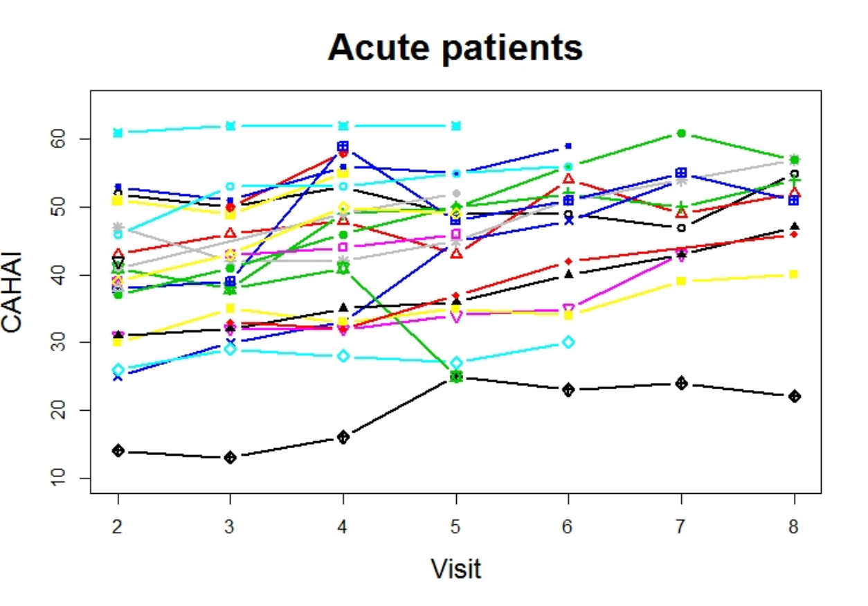
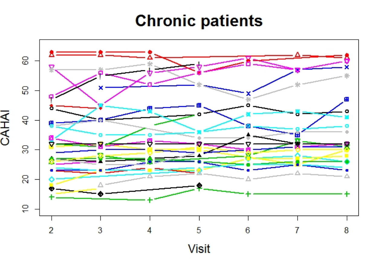
Based on the selected features, we \colorblack perform leave-one-patient-out cross validation on these two patient groups respectively using the linear fixed-effects model. As shown in Fig. 8, the prediction results of the chronic patients (with mean RMSE 3.29) tend to be much better than the ones of the acute group (with mean RMSE 7.24). One of the main reasons might be the nature of the patient group. In Fig. 9, we \colorblack plot the clinical CAHAI distribution (i.e., the ground truth CAHAI) from week 2 to week 8, and we can see the clinical CAHAI scores are very stable for chronic patients. On the other hand, for acute patients who suffered from stroke in the past 6 months, their health statuses were less stable and affected significantly by various factors, and in this case the simple linear fixed-effected model yields less promising results.


4.2.3 Performance of Longitudinal mixed-effects Model with Gaussian Process prior (LMGP)
We also \colorblack develop LMGP for both patient groups. We have applied different covariance kernels in LMGP models and found the one with powered exponential kernel achieves the best results. The following discussion will therefore focus on the model with this kernel. More results of using other kernels can be found in Appendix. 5.5.


Here, we \colorblack use the selected features (from Table 3) as the fixed-effects features and random-effects features. Similar to the linear fixed-effects model, we \colorblack evaluate the performance based on leave-one-patient-out cross validation, and the mean RMSE values \colorblack are reported in Fig. 10, from which can see LMGP can further reduce the errors when compared with the fixed-effects linear model, with mean RMSE 5.75 for acute patients and 3.12 for chronic patients, respectively.


Based on LMGP, we also \colorblack perform ”continuous monitoring”—with week-wise predicted CAHAI score — on 4 patients (two for each patient group) from week 2 to week 8, and the results \colorblack are reported (with mean and confidence interval) in Fig. 11, which is extremely helpful when uncertainty measurement is required.
4.2.4 On the fixed-effects part of LMGP
LMGP includes two key parts, i.e., the linear fixed-effects and the non-linear random-effects part, and it is important to choose the key features for modelling. Since the fixed-effects part measures the main (linear) relationship between the input features and the predicted CAHAI, we \colorblack study the corresponding feature subsets. For random-effects part, we \colorblack use the full LASSO features (as shown in Table 3).
To select the most important feature subset for the fixed-effects part modelling, we \colorblack rank the features (from Table 3) based on two criteria: LASSO coefficients, and correlation coefficients (between features and CAHAI, as described in Sec.4.1). Table 4 demonstrates ranked features, and here only the top features (i.e., top 3 features for acute patients and top 5 features for chronic patients) \colorblack are used to model the fixed-effects part, and the settings as well as the results \colorblack are reported in Table 5.
| - |
|
| ||||||||
|
|
| ||||||||
|
|
|
It is interesting to observe the performance may \colorblack vary when different feature subsets are applied. Specifically, with the top feature subsets, modelling the LMGP’s fixed-effects part can further reduce the errors \colorblack to some extent for acute patients, in contrast to chronic patients with increased errors. The top 5 features selected via the LASSO criterion yields the worst performance for chronic patients, and one possible explanation could be the lack of feature —–the initial health condition—–a major attribute for chronic patient modelling (see Fig. 9).
| Acute Patients |
|
|
RMSE | ||||
|
|
5.75 | |||||
|
|
5.37 | |||||
|
|
5.51 | |||||
| Chronic Patients |
|
|
RMSE | ||||
|
|
3.12 | |||||
|
|
3.20 | |||||
|
|
5.12 |
4.2.5 Model comparison
Based on our proposed (41-dimensional) stroke-rehab-driven features, we \colorblack compare LMGP with a number of classical predictive models, such as neural network (NN), support vector regression (SVR) and random forest regression(RF) for acute/chronic patient groups. It is worth noting that we cannot use the popular deep learning structures such as convolutional neural network(CNN) or recurrent neural network(RNN) on the time-series signal, due to the lack of frame-wise or sample-wise annotation. Yet with the stroke-rehab-driven features and trial-wise annotation, simple neural networks such as multi-layer perceptron(MLP) can be applied, and here we \colorblack use a 3-layer MLP.
| Predictive Models |
|
RMSE (Chronic) | |
| Neural Network | 10.50 | 4.93 | |
| Support vector regression (linear) | 7.47 | 3.25 | |
| Support vector regression (rbf) | 9.67 | 4.92 | |
| Random forest regression | 8.19 | 3.93 | |
| Linear fixed-effects model | 7.24 | 3.29 | |
| LMGP | 5.75 | 3.12 |
LOSO-CV \colorblack is applied with the mean RMSE values reported in Table 6, from which we \colorblack observe linear models (linear SVR and linear fixed-effects model) yield better results than non-linear methods (NN, SVR with rbf, and RF). One of the explanation is the over-fitting effect, where the trained non-linear models do not generalise well to the unseen patients/environments in this longitudinal study setting. RF is normally known as a classifier with high generalisation capability, yet it may suffer from the low-dimensionality of the selected features (6 features for acute patients and 10 features for chronic patients). Given the simplicity of the linear models and the designed low-dimensional features, linear models tend to suffer less from the over-fitting effect, with reasonable results in these challenging environments. \colorblack Compared with linear models, our LMGP can further model the longitudinal mixed-effects (i.e., with linear fixed-effect part and non-linear random-effects part), making the system adaptive to different subjects/time-slots, with the lowest errors.
| Methods |
|
RMSE (Chronic) | |
| Tang et al. Tang_stroke | 15.98 | 12.76 | |
| Halloran et al. Shane_ISWC | 10.12 | 12.14 | |
| Ours | 5.75 | 3.12 |
We also \colorblack compare our approach with other automated CAHAI score regression methods Tang_stroke Shane_ISWC in the existing literature. Different from our approach, Tang_stroke and Shane_ISWC are pure data-driven approaches. To address the lack of annotation problem, Tang et al. use GMM clustering (on the sliding windows) Tang_stroke to learn latent features that can be aggregated for trial-wise representation, while Halloran et al. Shane_ISWC employ pseudo labelling strategy for trial-wise representation. However, both data-driven features cannot suppress the substantial noises in the original accelerator signal, and such noises (e.g., irrelevant daily activities) significantly affect the performance of both approaches. In contrast, by taking advantage of the domain knowledge, our proposed stroke-rehab-driven representation is compact yet informative, and from Table 7 and Table 6 we can see it tends to have lower errors than Tang_stroke Shane_ISWC irrespective of the predictive models for both patient groups.
.
5 Conclusions
In this work, we \colorblack develop an automated stroke rehabilitation assessment system using wearable sensing and machine learning techniques. We \colorblack collect accelerometer data using wrist-worn sensors, based on which we \colorblack build models for CAHAI score prediction, which can provide objective and continuous rehabilitation assessment. To map the long time-series (i.e., 3-day accelerometer data) to the CAHAI score, we \colorblack propose a pipeline which \colorblack can perform from data cleaning, feature design, to predictive model development. Specifically, we \colorblack propose two compact features which can well capture the rehabilitation characteristics while suppressing the irrelevant daily activities, which is crucial on analysing the data collected in free-living environments. We further \colorblack use LMGP, which can make the model adaptive to different subjects and different time slots (across different weeks). Comprehensive experiments \colorblack are conducted on both acute/chronic patients, and very promising results \colorblack are achieved, especially on the chronic patient group. We also \colorblack study different feature subsets on modelling the fixed-effects part in LMGP, and experiments \colorblack suggest the errors can be further reduced for the challenging acute patient population.
Due to irrelevant daily activities and strong heterogeneity among subjects, it is very challenging for researchers in mathematics, computing sciences and other areas to deal with free-living data. It is also crucial to develop models which have good mathematical properties and have physical explanation particularly in medical research. Hopefully, the ideas of the new features and the models discussed in this paper can provide some hints on addressing similar problems in health research.
Appendix
black
5.1 List of Abbreviations/notations
- •
VM Signal vector magnitude
- •
DWT Discrete wavelet transform
- •
DWPT Discrete wavelet packet transform
- •
LMGP Longitudinal mixed-effects Gaussian process prior
- •
SAD Normalised Sum of Absolute value of the wavelet coefficients at different Decomposition scales
- •
PNP wavelet features that combine both Paralysed side and Non-Paralysed side
5.2 The CAHAI score form

5.3 Discrete wavelet transform and discrete wavelet packet transform
The DWT procedure includes two parts: decomposition and reconstruction. Decomposition part will be the main focus in this project. We now consider more details of the DWT using matrix algebra:
| (7) |
where is the output of matrix of DWT coefficients in different scales. is the orthonormal matrix containing different orthonormal wavelet bases (more details can be checked in Daubechies:2006 and waveletbook) and it satisfies . is the raw signal. The signal with length , the orthonormal matrix can be separated into J+1 submatrices, each of which can produce a partitioning of the vector of DWT coefficients in each scale j, j = 1,2,…, J. To be more specific, Eq(7) can be rewritten as follows:
| (8) |
where is a column vector of length representing the differences in adjacent weighted averages from scale 1 to scale J, is the last column contained in which has the same length with . is defined as detailed coefficients at scale j. contains the approximated coefficients at the J-th level. has dimension , where j = 1,2,…,J and has the same dimension with . Note that the rows of design orthonormal matrix depend on the decomposition level j-th. In other words, the value of J depends on the DWT decomposition scale of the raw signal. The maximum decomposition level j equals J since our signal has length .
We now further consider wavelet packet transform DWPT. The DWPT is the expansion of the discrete wavelet transformation. In DWT, each scale is calculated by passing only the previous wavelet approximated coefficients through discrete-time low and high pass quadrature mirror filters. However, in the DWPT, both the detailed and approximation coefficients are decomposed to create the full binary tree. More details can be found in waveletbook.
5.4 Commonly used wavelet features
In the discrete wavelet transform (DWT), represents DWT coefficients in the j-th decomposition scale. DWT can be written as , where is a column vector with length and , is the orthonormal matrix which satisfies and contains different filters. Due to the orthonormality of DWT, which means that and , shows energy in the DWT coefficients with decomposition level . Now the energy preserving condition can be written as:
| (9) |
where is our VM data (the signal vector magnitude of accelerometer data; see Sec.3.2) with length N, is the discrete wavelet transform decomposition level. denotes the detailed coefficient in scale j, and is a vector of length representing the differences in adjacent weighted averages from scale 1 to scale J. denotes the approximated coefficients in the Jth level and has the same length as . Based on the decomposition, each represents a special part of the energy in our VM data which relates to the certain frequency domain Preece:2009 waveletbook. Then the sample variance from waveletbook can be decomposed as:
| (10) |
The term represents the sample variance (corresponding to at different scales of DWT decomposition) in our VM data .
There are many wavelet features (e.g., Preece:2009) for the classification of dynamic activities from accelerometer data using DWT. On this basis, we extract the features from the energy preserving condition and sample variance mentioned previously.
We aim to look for the features which imply the recovery level among the stroke patients (see Sec.3.3). Now, we define the features in the j-th level discrete wavelet transform and discrete wavelet packet transform:
For the detailed coefficients at decomposition level j, presents its energy and the raw data with length N. Hence the physical explanation of is that it stands for the point energy at the decomposition level j. Moreover, from the Eq(10), represents the sample variance at the decomposition level j, also has properties of both the energy preserving condition and the sample variance in wavelet analysis with constant .
Comparing with (sum of Square value of DWT coefficients at scale (with normalisation)), we define other features call , which is sum of Absolute value of DWT coefficients at scale (with normalisation):
After we check the correlation between the important wavelet feature ( Sec.3.3) and CAHAI score, the branch of features using based perform better than those using based in Table 8. Hence we consider the commonly used feature in this paper.
| - | Acute | Patients | Chronic | Patients | ||||||||||||||||||||
| Scale (k) |
|
|
|
|
|
|
|
| ||||||||||||||||
| k=1.1 | 0.60 | -0.65 | 0.68 | -0.70 | 0.45 | -0.45 | 0.56 | -0.56 | ||||||||||||||||
| k=1.2 | 0.60 | -0.66 | 0.69 | -0.71 | 0.46 | -0.45 | 0.57 | -0.56 | ||||||||||||||||
| k=1.3 | 0.63 | -0.69 | 0.70 | -0.72 | 0.49 | -0.48 | 0.58 | -0.57 | ||||||||||||||||
| k=1.4 | 0.62 | -0.68 | 0.69 | -0.71 | 0.47 | -0.47 | 0.57 | -0.57 | ||||||||||||||||
| k=2 | 0.65 | -0.69 | 0.69 | -0.71 | 0.45 | -0.45 | 0.56 | -0.55 | ||||||||||||||||
| k=3 | 0.63 | -0.67 | 0.67 | -0.68 | 0.39 | -0.38 | 0.53 | -0.52 | ||||||||||||||||
| k=4 | 0.59 | -0.63 | 0.60 | -0.63 | 0.31 | -0.30 | 0.48 | -0.47 | ||||||||||||||||
| k=5 | 0.46 | -0.50 | 0.49 | -0.52 | 0.29 | -0.27 | 0.43 | -0.42 | ||||||||||||||||
| k=6 | 0.32 | -0.38 | 0.35 | -0.38 | 0.20 | -0.16 | 0.35 | -0.34 | ||||||||||||||||
| k=7 | 0.16 | -0.19 | 0.19 | -0.20 | 0.13 | -0.10 | 0.25 | -0.24 |
In our analysis, we assume the discrete wavelet decomposition level which is the same level as in Sekine:1998 and contains enough low-frequency component as the stroke patients’ movement. The frequency domain with seven scales is shown in Table 9:
| Scale 7 | Scale 6 | Scale 5 | |
| Frequency | 0.0078hz-0.0156hz | 0.0156hz - 0.0312hz | 0.0312hz - 0.0625hz |
| Scale 4 | Scale 3 | Scale 2 | |
| Frequency | 0.0625hz - 0.125hz | 0.125hz - 0.25hz | 0.25hz - 0.50h |
| Scale 1 | |||
| Frequency | 0.50hz - 1hz |
So far, we have decomposed the VM data X to get , , … , using DWT. Since the frequency domain at scale 1 is so wide (0.50hz - 1hz), it is better to divide it into smaller one, then using DWPT in Appendix 5.3, we can further decompose into , , and which are the results of the -rd stage of DWPT, each coefficient vector with length has the same dimension as the coefficients in the third level of DWT decomposition, that is
Now we have coefficients at 10 decomposition scales by using DWT and DWPT: , , , , , , , , and . Based on these detailed coefficients, we define the commonly used wavelet features again:
There are 10 features which provide reliable and valid information (corresponding to more frequency domains) from different frequency domains. The frequency domain of these features, among 10 scales, is listed in Table 10:
| Scale 1.1 | Scale 1.2 | Scale 1.3 | |
| Frequency | 0.5hz - 0.625hz | 0.625hz - 0.75hz | 0.75hz - 0.875hz |
| Scale 1.4 | Scale 2 | Scale 3 | |
| Frequency | 0.875hz - 1hz | 0.25-0.50hz | 0.125hz - 0.25hz |
| Scale 4 | Scale 5 | Scale 6 | |
| Frequency | 0.0625hz - 0.125hz | 0.0312hz - 0.0625hz | 0.0156hz - 0.0312hz |
| Scale 7 | |||
| Frequency | 0.0078hz - 0.0156hz |
5.5 Performance of LMGP through three different kernels
Three kernels \colorblack are used in LMGP, and they are linear kernel, powered exponential kernel and rational quadratic kernel. We \colorblack use the selected features (from Table 3) as the fixed-effects features and random-effects features, and the results \colorblack are reported in Table 11.
| Selected kernels in LMGP |
|
RMSE (Chronic) | |
| linear kernel | 5.89 | 3.13 | |
| powered exponential kernel | 5.75 | 3.12 | |
| rational quadratic kernel | 7.58 | 3.24 |
References
- [1] G. Donnan, M. Fisher, M. Macleod, and S. Davis. Stroke. Lancet, 371(2):1612–1623, 2008.
- [2] M. Wintermark, M. Sesay, E. Barbier, K. Borbély, W.P. Dillon, J.D. Eastwood, T.C. Glenn, C.B. Grandin, S. Pedraza, J.F. Soustiel, T. Nariai, G. Zaharchuk, J.M. Caillé, V. Dousset, and H. Yonas. Comparative overview of brain perfusion imaging techniques. Journal of Neuroradiology, 32(5):294–314, 2005.
- [3] Pietro Ferrari, Christine Friedenreich, and Charles Matthews. The role of measurement error in estimating levels of physical activity. American journal of epidemiology, 166:832–40, 11 2007.
- [4] Susan R Barreca, Paul W. Stratford, Cynthia L. Lambert, Lisa M. Masters, and David L Streiner. Test-retest reliability, validity, and sensitivity of the chedoke arm and hand activity inventory: a new measure of upper-limb function for survivors of stroke. Archives of physical medicine and rehabilitation, 86 8:1616–22, 2005.
- [5] S. Barreca, P. Stratford, C. Lambert, L. Masters, and D. Streiner. Test-Retest Reliability, Validity, and Sensitivity of the Chedoke Arm and Hand Activity Inventory: a New Measure of Upper-Limb Function for Survivors of Stroke. Arch Phys Med Rehabil, 86:1616–1622, 2005.
- [6] Andrew T. Walden Donald B. Percival. Wavelet methods for time series analysis. Cambridge Series in Statistical and Probabilistic Mathematics. Cambridge University Press, 1 edition, 2000.
- [7] S. J. Preece*, J. Y. Goulermas, L. P. J. Kenney, and D. Howard. A comparison of feature extraction methods for the classification of dynamic activities from accelerometer data. IEEE Transactions on Biomedical Engineering, 56(3):871–879, March 2009.
- [8] S. Barreca, P. Stratford, L. Masters, C. Lambert, J. Griffiths, and C. McBay. Validation of Three Shortened Versions of the Chedoke Arm and Hand Activity Inventory. Physiother. Can., 58:1–9, 2006.
- [9] Rana zia ur Rehman, Silvia Din, Yu Guan, Alison Yarnall, Jian Shi, and Lynn Rochester. Selecting clinically relevant gait characteristics for classification of early parkinson’s disease: A comprehensive machine learning approach. Scientific Reports, 9, 12 2019.
- [10] Nils Y. Hammerla, James M. Fisher, Peter Andras, Lynn Rochester, Richard Walker, and Thomas Ploetz. Pd disease state assessment in naturalistic environments using deep learning. In Proceedings of the Twenty-Ninth AAAI Conference on Artificial Intelligence, AAAI, pages 1742–1748. AAAI Press, 2015.
- [11] Thomas Ploetz, Nils Y. Hammerla, Agata Rozga, Andrea Reavis, Nathan Call, and Gregory D. Abowd. Automatic assessment of problem behavior in individuals with developmental disabilities. In Proceedings of the 2012 ACM Conference on Ubiquitous Computing, UbiComp, pages 391–400, New York, NY, USA, 2012. Association for Computing Machinery.
- [12] Bethany Little, Ossama Alshabrawy, Daniel Stow, I. Ferrier, Roisin McNaney, Daniel Jackson, Karim Ladha, Cassim Ladha, Thomas Ploetz, Jaume Bacardit, Patrick Olivier, Peter Gallagher, and John O’Brien. Deep learning-based automated speech detection as a marker of social functioning in late-life depression. Psychological Medicine, pages 1–10, 01 2020.
- [13] Bing Zhai, Ignacio Perez-Pozuelo, Emma A. D. Clifton, Joao Palotti, and Yu Guan. Making sense of sleep: Multimodal sleep stage classification in a large, diverse population using movement and cardiac sensing. Proc. ACM Interact. Mob. Wearable Ubiquitous Technol., 4(2), June 2020.
- [14] Akara Supratak, Hao Dong, Chao Wu, and Yike Guo. Deepsleepnet: a model for automatic sleep stage scoring based on raw single-channel eeg. IEEE Transactions on Neural Systems and Rehabilitation Engineering, PP, 03 2017.
- [15] Yang Bai, Yu Guan, and Wan-Fai Ng. Fatigue assessment using ecg and actigraphy sensors. In Proceedings of the 24rd International Symposium on Wearable Computers, ISWC, New York, NY, USA, 2020. Association for Computing Machinery.
- [16] Alzhraa A Ibrahim, Arne Küderle, Heiko Gaßner, Jochen Klucken, Bjoern M Eskofier, and Felix Kluge. Inertial sensor-based gait parameters reflect patient-reported fatigue in multiple sclerosis. Journal of neuroengineering and rehabilitation, 17(1):165, December 2020.
- [17] AM Ratcliffe, B Zhai, Y Guan, D Jackson, SWARM, and JR. Sneyd. Patient-centred measurement of recovery from day-case surgery using wrist worn accelerometers: a pilot and feasibility study. Anaesthesia, 2020.
- [18] Reed Gurchiek, Rebecca Choquette, Bruce Beynnon, James Slauterbeck, Timothy Tourville, Michael Toth, and Ryan McGinnis. Open-source remote gait analysis: A post-surgery patient monitoring application. Scientific reports, 9:17966, 11 2019.
- [19] Elham Dolatabadi, Ying Zhi, Bing Ye, Marge Coahran, Giorgia Lupinacci, Alex Mihailidis, Rosalie Wang, and Babak Taati. The toronto rehab stroke pose dataset to detect compensation during stroke rehabilitation therapy. pages 375–381, 05 2017.
- [20] A. C. Ganesh, B. S. Renganathan, C. Rajakumaran, S. P. Preejith, K. Shubham, J. Jayaraj, and S. Mohanasankar. Post-stroke rehabilitation monitoring using wireless surface electromyography: A case study. In 2018 IEEE International Symposium on Medical Measurements and Applications (MeMeA), pages 1–6, 2018.
- [21] H. Jung, J. Park, J. Jeong, T. Ryu, Y. Kim, and S. I. Lee. A wearable monitoring system for at-home stroke rehabilitation exercises: A preliminary study. In 2018 IEEE EMBS International Conference on Biomedical Health Informatics (BHI), pages 13–16, 2018.
- [22] Maxence Bobin, Franck Bimbard, Mehdi Boukallel, Margarita Anastassova, and Mehdi Ammi. Spectrum: Smart ecosystem for stroke patient’s upper limbs monitoring. 13, 02 2019.
- [23] Shane Halloran, Lin Tang, Yu Guan, Jian Qing Shi, and Janet Eyre. Remote monitoring of stroke patients’ rehabilitation using wearable accelerometers. In Proceedings of the 23rd International Symposium on Wearable Computers, ISWC 19, pages 72–77, New York, NY, USA, 2019. Association for Computing Machinery.
- [24] Lin Tang, Shane Halloran, Jian Qing Shi, Yu Guan, Chunzheng Cao, and Janet Eyre. Evaluating upper limb function after stroke using the free-living accelerometer data. Statistical Methods in Medical Research, 2020.
- [25] J.Q. Shi, B. Wang, E.J. Will, and R.M. West. Mixed-effects Gaussian process functional regression models with application to dose response curve prediction. Statistics in Medicine, 31(26):3165–3177, 2012.
- [26] J.Q. Shi, Y. Cheng, J. Serradilla, G. Morgan, C. Lambden, G. Ford, C. Price, H. Rodgers, T. Cassidy, L. Rochester, and J.A. Eyre. Evaluating Functional Ability of Upper Limbs after Stroke Using Video Game Data. In K. Imamura, S. Usui, T. Shirao, T. Kasamatsu, L. Schwabe, and N. Zhong, editors, International Conference on Brain and Health Informatics, volume 8211 of Lecture Notes in Artificial Intelligence, pages 181–192. Springer, 2013.
- [27] Axivity Ltd. AX3, 3-Axis Logging Accelerometer. https://axivity.com/product/ax3. [Online; accessed July-2020].
- [28] Aiden Doherty, Dan Jackson, Nils Hammerla, Thomas Ploetz, Patrick Olivier, Malcolm H. Granat, Tom White, Vincent T. van Hees, Michael I. Trenell, Christoper G. Owen, Stephen J. Preece, Rob Gillions, Simon Sheard, Tim Peakman, Soren Brage, and Nicholas J. Wareham. Large scale population assessment of physical activity using wrist worn accelerometers: The uk biobank study. PLOS ONE, 12(2):1–14, 02 2017.
- [29] Carlijn Bouten, Karel Koekkoek, Maarten Verduin, Rens Kodde, and Jan Janssen. A triaxial accelerometer and portable data processing unit for the assessment of daily physical activity. IEEE transactions on bio-medical engineering, 44:136–47, 04 1997.
- [30] Yu Guan and Thomas Ploetz. Ensembles of deep lstm learners for activity recognition using wearables. Proc. ACM Interact. Mob. Wearable Ubiquitous Technol., 1(2), June 2017.
- [31] T. Ploetz and Y. Guan. Deep learning for human activity recognition in mobile computing. Computer, 51(5):50–59, 2018.
- [32] Henrik [Stig Jørgensen], Hirofumi Nakayama, Hans Otto Raaschou, and Tom [Skyhøj Olsen]. Stroke: Neurologic and functional recovery the copenhagen stroke study. Physical Medicine and Rehabilitation Clinics of North America, 10(4):887 – 906, 1999. A New Century Approach to Stroke Management and Rehabilitation.
- [33] D. M. Karantonis, M. R. Narayanan, M. Mathie, N. H. Lovell, and B. G. Celler. Implementation of a real-time human movement classifier using a triaxial accelerometer for ambulatory monitoring. IEEE Transactions on Information Technology in Biomedicine, 10(1):156–167, 2006.
- [34] Yan Gao, Yang Long, Yu Guan, Anna Basu, Jessica Baggaley, and Thomas Ploetz. Towards reliable, automated general movement assessment for perinatal stroke screening in infants using wearable accelerometers. Proc. ACM Interact. Mob. Wearable Ubiquitous Technol., 3(1), March 2019.
- [35] Fouaz S Ayachi, Hung P Nguyen, Catherine Lavigne-Pelletier, Etienne Goubault, Patrick Boissy, and Christian Duval. Wavelet-based algorithm for auto-detection of daily living activities of older adults captured by multiple inertial measurement units (imus). Physiological measurement, 37(3):442–461, March 2016.
- [36] Jian Shi and Taeryon Choi. Gaussian Process Regression Analysis for Functional Data. London: Chapman and Hall/CRC, 01 2011.
- [37] I. Daubechies. Orthonormal bases of compactly supported wavelets. Commun. Pure. Appl. Math, pages 909–996, 2006.
- [38] M. Sekine, T. Tamura, M. Ogawa, T. Togawa, and Y. Fukui. Classification of acceleration waveform in a continuous walking record. In Proceedings of the 20th Annual International Conference of the IEEE Engineering in Medicine and Biology Society. Vol.20 Biomedical Engineering Towards the Year 2000 and Beyond (Cat. No.98CH36286), volume 3, pages 1523–1526 vol.3, Oct 1998.