Quantum scarring in a spin-boson system: fundamental families of periodic orbits
Abstract
As the name indicates, a periodic orbit is a solution for a dynamical system that repeats itself in time. In the regular regime, periodic orbits are stable, while in the chaotic regime, they become unstable. The presence of unstable periodic orbits is directly associated with the phenomenon of quantum scarring, which restricts the degree of delocalization of the eigenstates and leads to revivals in the dynamics. Here, we study the Dicke model in the superradiant phase and identify two sets of fundamental periodic orbits. This experimentally realizable atom-photon model is regular at low energies and chaotic at high energies. We study the effects of the periodic orbits in the structure of the eigenstates in both regular and chaotic regimes and obtain their quantized energies. We also introduce a measure to quantify how much scarred an eigenstate gets by each family of periodic orbits and compare the dynamics of initial coherent states close and away from those orbits.
I INTRODUCTION
The eigenstates of quantum systems that are fully chaotic in the classical limit may not be completely delocalized in the energy shell. This realization Heller 1984 came as a surprise, since in the classical domain the trajectories do fill the phase space densely. The presence of unstable periodic orbits (UPOs) plays a central role in the phase-space representation of the eigenstates Berry 1989. Despite having measure zero, UPOs give rise to quantum scars, which are characterized by enhanced probabilities along the phase-space region occupied by those orbits and thus prevent the uniform distribution of the eigenstates Heller 1991. Quantum scars were first studied in one-body systems McDonald and Kaufman 1979; Stöckmann 2006; Wintgen and Hönig 1989; D’Ariano et al. 1992; Heller 1987; Bogomolny 1988; Agam and Fishman 1993; Bohigas et al. 1993; Muller and Wintgen 1994; Kaplan and Heller 1998; Kaplan and Heller 1999; Wisniacki et al. 2006; Porter et al. 2017 and then in two-dimensional harmonic oscillators Keski-Rahkonen et al. 2019a; Keski-Rahkonen et al. 2019b and the Dicke model Dicke 1954; de Aguiar et al. 1992; Bakemeier et al. 2013. More recently, they have been connected also with some special non-thermal states of many-body quantum systems Turner et al. 2018; Turner et al. 2020, although in this case the analysis of the classical limit is still missing.
The present work focuses on the effects of quantum scars in the Dicke model. This spin-boson model consists of atoms collectively coupled with a quantized field. It was introduced to understand the superradiance phenomenon in light-matter systems Dicke 1954; Hepp and Lieb 1973a; Hepp and Lieb 1973b; Wang and Hioe 1973; Emary and Brandes 2003a; Garraway 2011 and it was later used in studies of nonequilibrium dynamics Pérez-Fernández et al. 2011; Altland and Haake 2012; Shen et al. 2017; Lerma-Hernández et al. 2018; Lerma-Hernández et al. 2019; Kloc et al. 2018; Kirton et al. 2019; Villaseñor et al. 2020, including the evolution of out-of-time-ordered correlators Chávez-Carlos et al. 2019; Lewis-Swan et al. 2019; Pilatowsky-Cameo et al. 2020a, and as a paradigm of the ultra-strong coupling regime in several systems De Bernardis et al. 2018; Frisk Kockum et al. 2019; Forn-Díaz et al. 2019; Le Boité. The model has been studied experimentally with cavity assisted Raman transitions Baden et al. 2014; Zhang et al. 2018, trapped ions Cohn et al. 2018; Safavi-Naini et al. 2018, and circuit quantum electrodynamics Jaako et al. 2016. It has two degrees of freedom and displays both regular and chaotic behavior Lewenkopf et al. 1991; Emary and Brandes 2003b; Emary and Brandes 2003a; Bastarrachea-Magnani et al. 2014a; Bastarrachea-Magnani et al. 2015; Bastarrachea-Magnani et al. 2016; Chávez-Carlos et al. 2016 depending on the Hamiltonian parameters and excitation energy. Scarring in the Dicke model was studied for a low number of atoms in de Aguiar et al. 1991; de Aguiar et al. 1992, where an algorithm to identify the classical periodic orbits (POs) was implemented. The technique allowed to match the phase-space probability accumulations of the eigenstates with specific POs. The comparison between quantum and classical phase-space distributions was later extended to a large number of atoms in Bakemeier et al. 2013.
Recently, in Pilatowsky-Cameo et al. 2020b we showed that even in the chaotic high-energy region, all eigenstates of the Dicke model accumulate around portions of the phase-space energy shells of the corresponding eigenenergies, covering at most half of the available phase space. This was done using a phase-space localization measure similar to the one studied in Ref. Wang and Robnik 2020.
In this work we identify the two fundamental families of POs that emanate from the two normal modes of the ground-state configuration and study extensively their influence in the phase-space localization of the eigenstates. The orbits change from stable in the regular low-energy regime of the model to unstable as one approaches the chaotic high-energy region. We introduce a measure that quantifies the degree of scarring of an eigenstate by a specific PO and use it to select the states concentrated around those two families of POs. We also show that the energies of these states follow the Bohr-Sommerfeld quantization rules for both stable and unstable POs.
The second part of the paper is dedicated to the dynamics of the Dicke model in the chaotic regime. The evolution depends on the proximity of the initial state to the POs. In the classical limit, an initial configuration launched exactly at a UPO will remain over it for an infinitely long time. However, the UPOs form a set of measure zero in the phase space, so their existence does not break the ergodic properties of the whole system and initial configurations picked up at random pass arbitrarily close to all other accessible configurations at the same energy foo a. In the quantum domain, the effects of the UPOs are more dramatic. An initial state defined over a phase space region that includes a short-period UPO should exhibit revivals and, after long times, it should be more likely to be found in the vicinity of that same UPO. Therefore, the state explores an effective reduced volume of the phase space Villaseñor et al. 2020 and displays what is known as a dynamical scar Tomiya et al. 2019 in its infinite-time average. In contrast, initial states that are away from short-period UPOs should follow a path to equilibrium according to random matrix theory, maximally covering the phase space at long times. Since we have two families of POs, we can choose initial coherent states that are very close to them and verify these expectations.
The paper is organized as follows. In Sec. II, we present the Dicke Hamiltonian, its properties, and its classical limit. In Sec. III, we identify the families of classical POs emanating from the ground-state configuration and introduce a measure to determine the degree of scarring of the eigenstates. In Sec. IV, we analyze the effects of scarring in the dynamics of initial coherent states close to those POs. Our conclusions are given in Sec. V.
II DICKE MODEL
The Dicke Hamiltonian Dicke 1954 is given by
| (1) |
where . The model describes a system of two-level atoms with atomic transition frequency interacting with a single mode of the electromagnetic field with radiation frequency . The parameter controls the atom-field coupling, () is the usual bosonic annihilation (creation) operator of the field mode, and are the collective pseudo-spin operators with being the Pauli matrices.
The eigenvalues of the squared total-spin operator determine the different invariant subspaces of the model. We use the symmetric atomic subspace defined by the maximum pseudo-spin value , which includes the ground state. The Hamiltonian commutes with the parity operator , where the operator has eigenvalues , that correspond to the total number of excitations. The number of photons is given by and the number of excited atoms by , where is an eigenvalue of the atomic operator .
When reaches the critical value , the Dicke model presents a second-order quantum phase transition Hepp and Lieb 1973a; Hepp and Lieb 1973b; Wang and Hioe 1973; Emary and Brandes 2003a. At this point, it goes from a normal phase (), where the ground state has no photons and all atoms are in their ground state, to a superradiant phase (), where the ground state has a finite amount of photons and excited atoms.
II.1 Classical limit of the Dicke Hamiltonian
The classical Hamiltonian defined over the four-dimensional phase space of the Dicke model, with coordinates , is constructed using Glauber-Bloch coherent states de Aguiar et al. 1991; de Aguiar et al. 1992; Bastarrachea-Magnani et al. 2014b; Bastarrachea-Magnani et al. 2014a; Bastarrachea-Magnani et al. 2015; Chávez-Carlos et al. 2016
| (2) |
which are built as a tensor product of Glauber coherent states for the bosonic sector
| (3) |
and Bloch coherent states for the pseudo-spin sector
| (4) |
where is the photon vacuum, and is the state with all atoms in their ground state. The raising (lowering) collective pseudo-spin operator, (), is defined in the usual way .
Taking the expectation value of the Hamiltonian under the states and dividing it by the pseudo-spin Villaseñor et al. 2020, we obtain the classical Hamiltonian
| (5) |
We define the rescaled energy corresponding to as
| (6) |
which determines an effective Planck constant Ribeiro et al. 2006.
Depending on the Hamiltonian parameters and excitation energies, different dynamical behaviors of the model are identified, ranging from regularity to chaos. As a case study, we choose , coupling parameter in the superradiant phase , and pseudo-spin value (). For these parameters, the ground-state energy is given by . The dynamics is regular up to a value of and chaotic for higher energies Chávez-Carlos et al. 2016.
III QUANTUM SCARRING
Quantum scarring is a phenomenon by which some eigenstates of a quantum system get concentrated around the UPOs that appear in the classical limit of the model. To identify the scarred eigenstates of the Dicke model, we must first identify the POs arising in the classical limit.
III.1 Families of periodic orbits in the classical limit
A PO with period is a subset of the phase space, such that
| (7) |
The most trivial periodic orbit consists of a single stationary point, where for all times . The classical dynamics given by yield several stationary points that may be located by finding the extrema of the Hamiltonian. For our chosen parameters, there are two stationary points located at the ground state energy Bastarrachea-Magnani et al. 2014b:
and , where the signs of and are opposite to those of . In our case,
| and |
We first consider , which is marked with a blue arrow in Figs. 1 (a1) and (a2), and with a red arrow in Figs. 1 (b1) and (b2).
By considering small displacements around the stationary point , we obtain two normal frequencies of the system, and , which are given by
where corresponds to the plus sign and to the minus sign. For our selection of parameters, and . Correspondingly, we have two normal periods and .
Let us focus first on the normal mode of period with the trivial PO . By perturbing this stable stationary point and using a monodromy method de Aguiar and Malta 1988 to guarantee the convergence, we can find a new PO with energy and period Weinstein 1973. This procedure can be successively repeated to increasing energies , so that a continuous family of periodic orbits is obtained all the way to the chaotic regime, where the orbits become unstable (see App. A for details). This family of POs is denoted by ,
| (8) |
and it is shown in Figs. 1 (a1) and (a2), where the color of each PO indicates its energy (lighter colors mean larger energies).
We repeat the procedure above for the other normal mode around the ground state with , yielding the POs of family ,
| (9) |
which is plotted in Figs. 1 (b1) and (b2).
The energy of each PO in the two families identified increases as the POs grow away from . In Fig. 1 (c), we show the period of the POs in (blue line) and for the POs in (red line) as a function of the energy . For a given energy , the period is between three and four times larger than , a feature to which we come back to when explaining our next results. In Fig. 1 (d), we display the Lyapunov exponents of those POs as a function of energy (see App. B for details). The orbits become unstable when the Lyapunov exponents are different from zero. Notice that for family , the Lyapunov exponent does not grow monotonically with the energy and there are ranges of high energies where the PO can be stable.
The classical Hamiltonian (5) is invariant under the transformation . This is the classical manifestation of the parity conservation present in the quantum system. The invariance means that if is a PO, we may find another PO by mirroring
where has the same period, energy, and Lyapunov exponent as . This transformation yields the mirrored families
| and | (10) |
The two families and are the ones that emanate from the stationary point .
III.2 Scarring of energy eigenstates
The four families , , , and scar many of the quantum eigenstates, as we show in this subsection.
III.2.1 Measure of scarring degree
The Husimi function of a state can be used to visualize how it is distributed in the phase space. Thus, in order to find the eigenstates scarred by those families of POs, we make use of the (unnormalized) Husimi function of a state ,
| (11) |
where is the coherent state centered at . In the case of a pure state , the function reduces to
| (12) |
To quantify the degree of scarring of a given state by a specific PO, we consider the temporal average of the state’s Husimi function along that PO. For a state and the PO with period , we define the quantity
| (13) |
where and any initial point can be used to perform the average. This measure is similar to the tube phase-space projection introduced in Ref. Kaplan and Heller 1998, but now taking into account the temporal behavior of the orbit. From the definition, we have that
| (14) |
where
| (15) |
is a tubular Gaussian distribution around the PO and is the coherent state centered at the point . See App. C for an illustration of the Husimi function of .
From Eq. (14), we can see that is the overlap of state with . To construct a baseline to compare the value of with, we consider a totally delocalized state
| (16) |
comprised of all the coherent states within a single energy shell at , where is the phase-space volume of the energy shell at . The value of the trace gives the overlap between a totally delocalized state and the orbit. By defining
| (17) |
we obtain a direct measure of quantum scarring. A value of indicates that the overlap between state and the PO is equal to that of a totally delocalized state. Values greater than indicate that the state is scarred by the PO . A value of , for example, says that state is twice as likely to be found near the PO as compared to the delocalized state . Values less than signal that state is less likely to be found near the PO than a fully delocalized state. This avoidance of a specific PO may be regarded as an “anti-scarring” effect.
We may quantify how much a state is scarred by the POs of the families described in Sec. III.1 by defining the numbers
| and | (18) |
for any energy . In words, measures how much populates the region of the phase space visited by the POs of families and at the energy , while does the same for the families and .
III.2.2 Overlap of the energy eigenstates with classical periodic orbits
 |
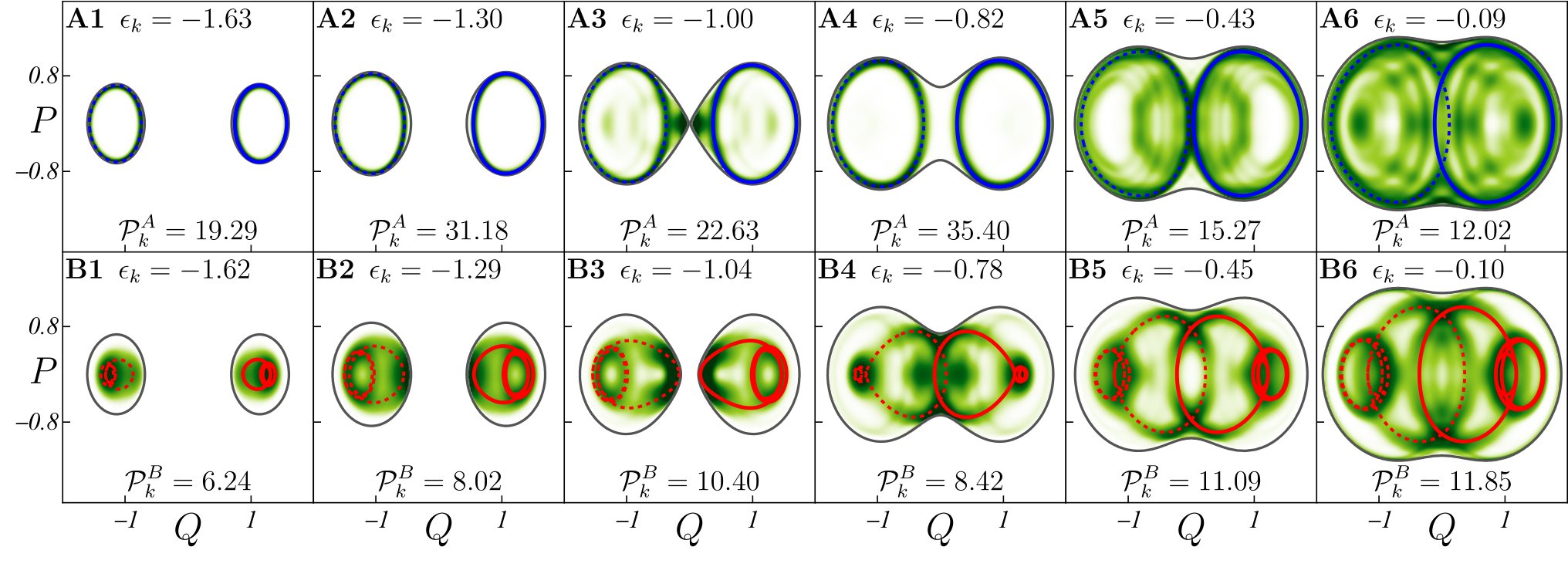 |
Bottom panels A1-B6: The green shades indicate the projected Husimi distribution for the corresponding eigenstates marked in panels (a) and (b) (darker colors indicate higher values). The gray curved outlines mark the border of the energy shell. The colored lines in the panels A1-B6 draw the POs: (solid blue), (solid red), (dashed blue), (dashed red). The value of and for the corresponding eigenstate are shown in each panel.
For an eigenstate of the Dicke Hamiltonian with scaled eigenenergy , the numbers
| and | (19) |
measure the scarring produced by the orbits of families and , respectively foo b.
In Fig. 2, we show the expectation value of the operator for each energy eigenstate, leading to an arrangement known as a Peres lattice Peres 1984; Bastarrachea-Magnani et al. 2014a. This is a convenient way to get information about all the eigenstates in a single picture. In the low-energy regime the points are clearly separated and arranged in a lattice-like fashion, but as the energy increases the structure gets destroyed and the number of points becomes much denser, as typical of chaotic systems. In Fig. 2 (a), we color the points according to the degree of scarring of each eigenstate by the family , that is, according to the value of . The same is done in Fig. 2 (b) for family using now .
As the phase-space distribution of a scarred state is close to a PO, the expectation value of the observable should be similar to the average of the classical variable over the PO. In Fig. 2 (a) and Fig. 2 (b), we plot with blue and red thick lines the value of the classical average
| (20) |
over each PO from family (blue) and (red), where is the period of . We see in Fig. 2 (a) [Fig. 2 (b)] that for the low energies in the regular regime, the eigenstates with a high value of [] lie very close to this blue [red] line.
Using the Bohr-Sommerfeld quantization rule, we semiclassically quantize the energies of the families and . Beginning from the ground-state energy , we successively find the excited energies by applying the quantization condition,
| (21) |
We plot the obtained energies [] with vertical thin blue [red] lines in Fig. 2 (a) [Fig. 2 (b)]. These vertical lines coincide perfectly with the individual eigenstates scarred by the POs of the families and in the low-energy region, where the POs are stable. As the energy increases and the POs become unstable, we find clusters of scarred eigenstates distributed around the semiclassical energies. According to Gutzwiller trace formula for the density of states Gutzwiller 1971 and also to Ref. Heller 1991, the width of these clusters should be given by the Lyapunov exponent of the PO at the respective energy, which is indeed confirmed by the horizontal bars shown at the bottom of Fig. 2 (a) and Fig. 2 (b), whose width is twice the value of the Lyapunov exponents of (blue) and (red) multiplied by .
The distribution of scarred states in the spectrum is governed by two numbers: (i) the periods of the POs determine the semiclassically quantized energies around which clusters of scarred states appear, and (ii) the Lyapunov exponents control the width of these clusters. These two numbers behave differently for families and as explained below.
- (i)
The periods of the POs in family are between three and four times shorter than those of . This has two consequences, is higher than and there is a smaller number of eigenstates scarred by family as compared to . The former occurs because the POs from family are shorter in the phase space than those from family , thus having smaller overlaps with a delocalized state. Since the denominator in in Eq. (17) is the overlap of the PO with a delocalized state, this results in the values of being between three to four times higher than . The latter occurs because a shorter period translates in greater energy separations . Thus, there are approximately four times more red vertical lines in Fig. 2 (b), marking , than blue vertical lines in Fig. 2 (a), marking . Because scarred eigenstates appear close to these energies, this results in more states scarred by family than states scarred by family .
- (ii)
The Lyapunov times of the POs in family are always much larger than their periods, which reflects the fact that the energy differences are larger than the Lyapunov exponents multiplied by . For family , the period of its POs in the chaotic region are only slightly shorter than the respective Lyapunov times. This allows us to clearly identify the clusters of eigenstates scarred by family around the semiclassical energies in Fig. 2 (a), but makes it harder to distinguish the ones scarred by around in Fig. 2 (b), because neighboring clusters may overlap.
We close Sec. III.2.2 with the interesting observation that POs from both families may affect the same eigenstate. In Fig. 2 (a) [Fig. 2 (b)], the blue circles outlined by red [red circles outlined by blue] mark the eigenstates where both and are greater than . These five states are located at energies where the semiclassical quantizations of both families coincide.
III.2.3 Projected Husimi distribution
We now use the Husimi distribution to visually confirm that the energy eigenstates with large values of and are scarred by the classical POs of families and .
For a state and energy , we consider the projection of the Husimi function over the classical energy shell by integrating out the bosonic variables ,
| (22) |
where . For an eigenstate , the projection yields a function depending only on the variables , which can be compared with the projection of the POs over the same plane - (see App. D for details on the computation of this projection).
We select 12 energy eigenstates Pilatowsky-Cameo et al. 2020b, marked as A1-A6 and B1-B6 in Fig. 2 (a) and Figs. 2 (b), which in addition to having high values of lie close to the classical average of given by Eq. (20). We plot the Husimi projection for each one of these eigenstates at the 12 bottom panels of Fig. 2. These distributions are superposed by the projections of the POs (blue solid line), (red solid line), (blue dashed line), and (red dashed line). Scarring is clearly visible in all panels. The quantum states A1-A6 and B1-B6 are highly concentrated around the classical periodic orbits. This happens even in the chaotic region of high excitation energy, as seen for A5, A6, B5, and B6 with , where the classical dynamics is ergodic
Interesting features are revealed by the juxtaposition of the Husimi projections and the periodic orbits. For example, the eigenstate B3 shows a significant concentration of probability towards the center at . This is because close to the energy of this state, specifically at and , there is an unstable stationary point and so the dynamics of the periodic orbit slows down around it. This gets reflected in the eigenstate by the localization of the Husimi distribution in the same region [see Fig. 6 (b) in App. C for an illustration of this effect]. Also noticeable is the fact that the probability distributions of the eigenstates A5 and A6 are not entirely confined to the periodic orbit, but extend beyond it, which contrasts with the high density concentration of the eigenstates A1-A4. This results in lower values of for A5 and A6 as compared to A1-A4.
IV SCARRING AND DYNAMICS
In this section, we show the effects that the scarred states have over the dynamical properties of non-stationary states. We consider three initial Glauber-Bloch coherent states that have energy in the chaotic regime. One is centered in a point of a UPO of family , one in a point of a UPO of family , and the third one is away from the POs of the identified families , , , and .

IV.1 Initial coherent states
We expand the selected coherent states in the Hamiltonian eigenbasis
| (23) |
The amplitudes and the degree of scarring of the corresponding eigenstates determine the dynamical properties of the initial states.
We consider three initial coherent states, , , and , where
| (24) | ||||
They all have mean energy in the chaotic region, , and the widths of their energy distributions in the energy eigenbasis are (in units of ) Schliemann 2015; Lerma-Hernández et al. 2018. The points , , and are marked with little circles in Figs. 1 (a1), (a2), (b1), and (b2). They all have the same shade of green indicating their equal energy. The point sits on top of the PO of family that has that same energy , as can be seen in Figs. 1 (a1) and (a2). The point sits on top of the PO of , as shown in Figs. 1 (b1) and (b2). The point is located far away from the POs of both families (and the mirrored families), as seen in Figs. 1 (a1), (a2), (b1), and (b2).
IV.1.1 Scarring of coherent states
| (25) |
of the initial coherent states [Figs. 3 (ai) and (bi)], [Figs. 3 (aii) and (bii)], and [Figs. 3 (aiii) and (biii)]. These distributions are usually referred to as local density of states (LDoS). In a sense, Figs. 3 (ai)-(biii) are similar to Figs. 2 (a) and (b), but now instead of in the vertical axis, we have the components of the chosen coherent states. The distributions in Figs. 3 (ai)-(aiii) are the same as in Figs. 3 (bi)-(biii), what changes is just the colors: the blue tones in Figs. 3 (ai)-(aiii) indicate the values of and the red tones in Figs. 3 (bi)-(biii) indicate the values of [see Eq. (19)]. In addition to the circles corresponding to amplitudes of the weights , Figs. 3 (ai)-(aiii) [Figs. 3 (bi)-(biii)] also display vertical lines that mark the semiclassically quantized energies [] given by Eq. (21).
We observe the following features for the three initial coherent states:
- (i)
For the initial coherent state located in the PO of family , the largest components , indicated as i1-i6 in Fig. 3 (ai), correspond to the eigenstates with large values of and therefore scarred by the POs of family . Due to the high participation of these eigenstates, we say that the initial coherent state is itself scarred by family . As visible in Fig. 3 (ai), the LDoS of exhibits a clear comb-like pattern, which is typical of scarred states Heller 1991. As seen in Fig. 2 (a), the scarred eigenstates cluster around the semiclassical energies . Because these scarred eigenstates give the largest contributions to the initial state, that is they lead to the biggest components , the LDoS attains higher values around the energies , creating the comb-like structure.
One sees that the contributions to from eigenstates non-scarred by the POs of family are erratically distributed, with small and medium values of , as evident from the red points in Fig. 3 (bi), which mark the eigenstates according to their values of .
- (ii)
A similar picture emerges for the initial coherent state located in the PO of family . Its largest components , indicated as ii1-ii6 in Fig. 3 (bii), correspond to the eigenstates with large values of and thus scarred by the POs of family . The contributions from eigenstates non-scarred by this family are smaller and their values fluctuate randomly. The initial coherent state is therefore scarred by family . Its comb-like structure is somewhat visible, but, because the separations are of the order of the Lyapunov exponents of the POs in family , it is harder to distinguish it.
As discussed in the previous section, there are more eigenstates scarred by family than by family , due to the difference in the periods of the POs between the two families. This difference between the two families is evident if we compare the number of blue circles in Fig. 3 (ai) with the number of red circles in Fig. 3 (bii). The larger number of contributing states from family explains why the biggest components in Fig. 3 (bii) are smaller than the ones in Fig. 3 (ai).
- (iii)
For the initial coherent state , which is located far away from the POs of families , , and , the largest components , indicated as iii1-iii6 in Figs. 3 (aiii) and (biii), are not colored by any of the two families, as expected.
In Figs. 3 (ci)-(ciii), we plot the same Peres lattice of the pseudo-spin operator that we showed in Fig. 2, but we now use tones of green to indicate the values of for the coherent states [Fig. 3 (ci)], [Fig. 3 (cii)], and [Fig. 3 (ciii)]. The panels make it evident that the components of the three initial states, all covering a wide range of energies within the chaotic regime, are actually localized in different regions of the lattice. The components of () concentrate towards the top (bottom) of the lattice, because this is where the eigenstates scarred by family () tend to be found, closer to the classical average of (Eq. (20)) over the corresponding family [blue (red) line in Figs. 3 (ci)-(ciii)]. The components of spread more homogeneously over the middle part of the lattice, as seen in Fig. 3 (ciii).

IV.1.2 Husimi distributions of the most contributing eigenstates
In Fig. 4, we plot the projected Husimi distributions for each of the six eigenstates with the largest components in the LDoS of the initial coherent states [Figs. 4 (i1)-(i6)], [Figs. 4 (ii1)-(ii6)], and [Figs. 4 (iii1)-(iii6)]. This is done in two different ways:
(a) By first intersecting the Husimi distribution of the eigenstate with the energy shell at the respective eigenenergy , and then integrating over (,), as we did in Fig. 2 A1-B6 [see Eq. (22)] and in Pilatowsky-Cameo et al. 2020b. This choice is shown in green in the top of each panel of Fig. 4.
(b) By directly integrating over the bosonic variables of the Husimi function, , as done in de Aguiar et al. 1991; Furuya et al. 1992; Wang and Robnik 2020. This alternative is plotted in orange in the bottom of each panel of Fig. 4.
As expected, the Husimi functions of the eigenstates i1-i6 [ii1-ii6] with the largest components in the coherent state [] concentrate along the POs of family [] at the corresponding energy. This is more evident with the Husimi functions intersected by the energy shells (top green plots in Fig. 4) than in the complete projected Husimi functions (bottom orange plots in Fig. 4), which are more blurred, because they include all energy shells. This difference shows the advantage of the projection method (a), which makes it easier to distinguish the outline of the POs. Method (a) was first developed in Pilatowsky-Cameo et al. 2020b and more details are given in App. D.
Similarly to the eigenstates i1-i6 and ii1-ii6, the Husimi functions of the eigenstates iii1-iii6 that contribute the most to the initial state are not smoothly distributed either. As seen in Figs. 4 (iii1)-(iii2), the visible concentrations in parts of the phase space suggest that these eigenstates are also scarred by one or more families of POs , although they are different from the families and .
IV.2 Survival probability of coherent states
To study the dynamics of the three selected initial states, we consider the survival probability defined as
| (26) |
where is the unitary evolution operator. measures the probability of the evolved state to return to its initial state for any given time. By expanding the coherent state in the Hamiltonian eigenbasis as in Eq. (23), we can rewrite the survival probability as
| (27) |
which can also be written in an integral form,
| (28) |
which is the squared norm of the Fourier transform of the LDoS, as defined in Eq. (25).
In general, the evolution of scarred initial states, where the LDoS is fragmented, produces partial revivals at times before the Lyapunov time Heller 1984 and the saturation values of the survival probability are larger than those for non-scarred states Kaplan and Heller 1998; Villaseñor et al. 2020. The reason for this behavior is, of course, the low number of eigenstates that contribute to the dynamics.

The survival probability of the initial coherent states , , and are respectively shown in Figs. 5 (ai)-(bi), Figs. 5 (aii)-(bii), and Figs. 5 (aiii)-(biii). The orange curves are numerical results and the thick purple ones are running averages. The initial decay of for the three cases is Gaussian, since the envelope of the LDoS is Gaussian, and it then reaches values close to zero, as explained in Villaseñor et al. 2020. The subsequent behavior differs among the three states.
For state , the first revival of the survival probability occurs at [Fig. 5 (bi)], which is precisely the average of the periods within the energy range of state , . A second revival is observed at , while the next ones do not follow this period, because changes strongly through the energy range of state destroying the periodicity. This may be seen in the left inset of Fig. 1 (c), where the little blue square marks the value of . For longer times, the survival probability equilibrates, fluctuating around its asymptotic value drawn with a horizontal black dashed line Villaseñor et al. 2020.
The first revival of for state appears at [Fig. 5 (bii)], which corresponds to the average period of the POs in the family within the energy range of state . The subsequent revivals happens at multiples of this period. The periods do not vary as much as around , as seen in the right inset of Fig. 1 (c), where the value is marked with a little red square. The slope of around is large, while actually attains a local minimum close to . As a result, the revivals of the survival probability of state follow the period for much longer than in the case of state .
A great advantage of having identified the families and is that we know why and where the revivals should happen. Having access to the number of contributing eigenstates and knowing why there are more contributing states from family than from family help us understand also why the survival probability for the initial state saturates at a lower point than for the state .
In contrast to states and , the initial coherent state does not show revivals. Instead, the survival probability shows a behavior similar to what we obtain when considering an initial state where the coefficients are random numbers. This latter case is indicated with a green line in Fig. 5 (aiii) and Fig. 5 (biii) and it is well described using random matrix theory Lerma-Hernández et al. 2019; Villaseñor et al. 2020.
A complete picture of the frequencies dominating the dynamical behavior of the coherent states may be obtained by calculating the inverse Fourier transform of the survival probability,
| (29) |
which is the autocorrelation function of the LDoS. This function gives us the distribution of frequencies of the survival probability in units of . In Figs. 5 (ci), (cii), and (ciii), we plot with black bars for states , , and , respectively. The vertical blue [red] lines in Fig. 5 (ci) [Fig. 5 (cii)] mark the integer multiples of the energy separation [] corresponding to the period []. In Fig. 5 (ci) [Fig. 5 (cii)], the function displays a comb-like pattern following the energy separation above, indicating that the period [] indeed dominates the behavior of the survival probability of state []. Figure 5 (ciii), on the other hand, does not exhibit any recognizable pattern. Because is the autocorrelation function of the LDoS (Eq. 29), it enhances any periodic structure present in . This amplifies the comb-like structures that is present in the LDoS of states and , and confirms that such a structure is absent in the LDoS of state .
The fact that the survival probability of state is so well described by random matrix theory and that no frequencies clearly stand out in its Fourier transform is puzzling at first sight, since Figs. 4 (iii1)-(iii6) suggest that the most contributing eigenstates to , that is eigenstates iii1-iii6 in Figs. 3 (aiii) and (biii), are also scarred. What we have come to understand from the analysis of various initial states is that the onset of revivals depends on two factors: the eigenstates with the largest participations in the LDoS should be scarred by the same family of POs, so that the periods of the POs generating the scars are similar; and these periods should be small in comparison to the Lyapunov times. For a given family of POs, if the Lyapunov time is shorter than the period, the revival does not have time to develop before saturation. This happens if either the PO is very unstable or if it has a very long period. It may therefore be that the eigenstates iii1-iii6 either do not belong to the same family and thus the corresponding POs have very dissimilar periods, or that these periods are so long that the revivals are unable to manifest. These are, however, open questions that can only be answered with the identification of the families associated with those states.
IV.3 Dynamical scarring
We finally analyze how the scarring manifests in the infinite-time average of the coherent states Pilatowsky-Cameo et al. 2020b
| (30) |
With the functions and defined by Eq. (18), we may calculate
Notice that and are particularly large, while the rest of the numbers are less or approximately equal to . This means that, at any time , state [] is more likely to be found in the vicinity of the orbits of families and [ and ] at energy than what one would expect for a state that is completely delocalized in the energy shell. This effect is known as dynamical scarring Tomiya et al. 2019.
We can visualize the dynamical scars by calculating the projected Husimi distributions [Eq. (22)] of the infinite-time averages , , and . These are plotted in Figs. 5 (di), (dii), and (diii), respectively. The dark concentrations in Fig. 5 (di) follow the orbit of family () at energy shown with a blue solid (dashed) line. The concentrations in Fig. 5 (dii) follow the orbit from () at the same energy shown with a solid (dashed) red line. Interestingly, some dark concentrations are visible also in Fig. 5 (diii), which suggest that state is scarred, but by POs from families other than those identified in this work.
The fact that the survival probability of state is so well described by random matrix theory [green line in Fig. 5 (aiii) and Fig. 5 (biii)] and no identifiable structure is visible in the autocorrelation of its LDoS [Fig. 5 (ciii) and Eq. (29))] suggests that even though this state has a minor degree of scarring that is visible in phase space [Fig. 5 (diii)], it is not identifiable by just looking in the Hilbert space. To better understand this feature, we use the ratio between the asymptotic value of the survival probability of and the asymtpotic value of the survival probability of an ensemble of random states with the same enveloping LDoS Villaseñor et al. 2020,
| (31) |
The ratio measures the similarity between the LDoS of the coherent state and that of a random state, (see Ref. Villaseñor et al. 2020 for an extensive discussion of ). A ratio indicates that these distributions are very similar. Lower values imply that there are periodic structures in the LDoS of the chosen coherent states, which are, evidently, absent in the LDoS of a random state Lerma-Hernández et al. 2019. For states and , and , respectively, while for state . These numbers show that the scarring can be traced back to a comb-like structure in the LDoS of states and , but not of state . This is consistent with Ref. Pilatowsky-Cameo et al. 2020b, where we found concentrations resembling dynamical scars in the phase-space projections of even the most random-like coherent states at energy , which display no revivals, no comb-like structures in their LDoS, and a path to equilibrium well-described by random matrix theory.
The dynamical behavior of the survival probability of the coherent states can be described by two competing effects. Periodic structures in the LDoS give rise to revivals, while random-like spreading within the Gaussian envelope of the LDoS prevents revivals. In between the two cases, one may find coherent states whose LDoS display a slightly larger participation of some eigenstates separated by a nearly constant energy difference, but this periodic structure does not stand out significantly over the Gaussian envelope, so revivals are not observed. Yet, when one performs infinite-time averages, the scars corresponding to the high participating eigenstates become visible as in Fig. 5 (diii). A complete description of this kind of coherent states requires the challenging task of identifying the family, or set of families, of POs that scar those high participating eigenstates, so that one can compare their Lyapunov times and periods. This is an interesting idea for a future work.
V CONCLUSIONS
We identified the two fundamental families of classical periodic orbits (POs) that emanate from the ground state of the Dicke model in the superradiant phase and extensively explored their effects in the quantum domain. By introducing a measure of scarring based on the temporal average of the Husimi function of an eigenstate along a PO, we were able to identify which eigenstates are scarred by which family of POs, and by projecting the Husimi functions over the energy shell corresponding to the energy of the eigenstate, we found an effective way to visualize the concentrations around the POs of those families.
We also showed that knowledge of the periods and Lyapunov exponents of the POs in the two identified families allows us to characterize the distribution of scarred eigenstates. The energies of the eigenstates scarred by the two families cluster around values obtained by means of the Bohr-Sommerfeld quantization rule of the periods, and the width of these clusters is directly related to the Lyapunov exponents of the POs generating the scars.
The dynamical consequences of the presence of eigenstates scarred by the two identified families were studied by considering the survival probability of three representative initial coherent states, two localized in the vicinity of the POs of the two families and one away from them. For the two states close to the POs, our detailed knowledge of the families allowed us to understand the revivals, their periods, and the saturation values of the survival probability. By performing the infinite-time averages of the density matrices of these initial coherent states, dynamical scars were observed. The third initial state shows a survival probability and a local density of states akin to those of random initial states, even though the dynamics has contributions from eigenstates scarred by families not identified here. The fact that the potential families associated with these scars are unknown to us prevents us from making conclusive statements about this state.
An important extension of the present study would be the systematic identification of more families of POs and the analysis of how they influence the spectrum and dynamics of the model.
ACKNOWLEDGMENTS
We thank D. Wisniacki for his valuable comments and acknowledge the support of the Computation Center - ICN, in particular of Enrique Palacios, Luciano Díaz, and Eduardo Murrieta. SP-C, DV and JGH acknowledge financial support from the DGAPA- UNAM project IN104020, and SL-H from the Mexican CONACyT project CB2015-01/255702. LFS was supported by the NSF grant No. DMR-1936006.
Appendix A Algorithm to find families of periodic orbits emanating from stationary stable points
Given a stable stationary point with energy and normal period , we iteratively find a continuous family of POs starting from . The existence of these families is guaranteed by theorem 2.1 of Ref. Weinstein 1973.
First, we detail a variant of an algorithm known as the monodromy method Baranger et al. 1988; de Aguiar and Malta 1988. This is a Newton-Raphson-type algorithm that converges towards a PO given an initial guess for an initial condition and period. This type of algorithms has been extensively studied in several systems. See, for example, Refs. Simonović 1999; de Aguiar et al. 1992. Then, we detail an algorithm to iteratively construct the guesses required to find the POs.
A.1 The monodromy method: converging to a periodic orbit given a good initial guess
Assume we have guesses and for an initial condition and period of a PO, respectively. We want and , the initial condition and period of an orbit in the same energy shell as . Denote by the fundamental matrix associated to the Hamiltonian system and the Hamiltonian flow satisfying (See Gaspard 1998 1.1.3). If is small, one may approximate to first order,
Similarly, if is small, Taylor expanding the flow up to first order,
where is the gradient of the Hamiltonian. Then, we have
| (32) | ||||
where . Thus, we can approximate the periodicity constriction to first order by
| (33) |
Also, we can approximate the energy constriction to first order to get
| (34) |
and, finally, the constriction to stay in the same Poincaré section of constant as
| (35) |
where . This last constriction eliminates movement along the flow and increases the stability of the algorithm.
The linear constrictions (33), (34) and (35), may be written in matrix form as
This overdetermined system of linear equations may be approximately solved by least squares using Moore-Penrose pseudoinversion. The solution for and is not exact, but the process may be iterated with new guesses and that will converge to and if the initial guesses were good enough.
A.2 Finding families of periodic orbits
We now define an iterative process to find the families of POs. For the first step, we start with a stable stationary point with energy and normal period .
Given , we now explain how to find with close to . Pick and define a perturbation , where is a scalar such that . For the first step, , in which case one may select any direction (we use the direction), and the stability of the initial stationary point will guarantee that the algorithm converges. Set
| and | (36) |
where
where and are the energy and period of the closest previously calculated orbit. This way, is linear extrapolation based on the behavior of the previous orbits.
Using the monodromy method detailed in the previous subsection, we may correct the guesses and to obtain actual solutions and so that the desired PO is
| (37) |
Although energy is constrained in the monodromy method we used, this is only to first order, so may not be exactly equal to . This is easily fixed by performing additional iterations with smaller which converge to the desired energy.
Appendix B Computation of the Lyapunov exponent of a periodic orbit
For any point of the phase space , the associated maximal Lyapunov exponent may be calculated with the spectral norm of the fundamental matrix, , which is the square root of the maximal eigenvalue of the symmetric matrix . The formula reads Gaspard 1998; Chávez-Carlos et al. 2019; Pilatowsky-Cameo et al. 2020a
| (38) |
In the case that corresponds to a periodic condition of period , Eq. (38) is greatly simplified. The so-called monodromy matrix associated to is . Then for all positive integers Gaspard 1998. Thus,
| (39) |
where . In Ref. Pilatowsky-Cameo et al. 2020a, it was shown that the rightmost limit of Eq. (39) is equal to . That is the maximal real part of the eigenvalues of , which are given by , where are the eigenvalues of . Thus,
| (40) |
In short, finding the maximal Lyapunov exponent of a periodic orbit of period reduces to computing the monodromy matrix , which is done by simple numeric integration, and then taking the greatest of the norms of its eigenvalues divided by .
Appendix C The Husimi distribution along periodic orbits
The unnormalized Husimi function for a coherent state , as given by Eq. (12), is very well fitted by
| (41) |
for values of larger than . The distance reads
where , and are the spherical coordinates for the Bloch sphere, and . Inserting Eq. (41) into Eq. (15), we get
| (42) |
for any initial .

As an illustration, we plot in Fig. 6 the Husimi function of for two generic POs.
Appendix D Computation of projected Husimi distribution
Because of the properties of the function, Eq. (22) equals
| (43) |
where are the two solutions in of the second-degree equation , are the two solutions in of the second-degree equation , and
| (44) |
We compute the integral (43) with a Chebyshev-Gauss quadrature method. Pilatowsky-Cameo et al. 2020b
References
- Heller (1984) Eric J. Heller, “Bound-state eigenfunctions of classically chaotic Hamiltonian systems: Scars of periodic orbits,” Phys. Rev. Lett. 53, 1515–1518 (1984).
- Berry (1989) Michael Victor Berry, “Quantum scars of classical closed orbits in phase space,” Proceedings of the Royal Society of London. A. Mathematical and Physical Sciences 423, 219–231 (1989).
- Heller (1991) E. J. Heller, “Wavepacket dynamics and quantum chaology,” in Les Houches Summer School 1991 on Chaos and Quantum Physics, edited by M.-J. Giannoni, A. Voros, and J. Zinn Justin (Springer, 1991).
- McDonald and Kaufman (1979) Steven W. McDonald and Allan N. Kaufman, “Spectrum and eigenfunctions for a Hamiltonian with stochastic trajectories,” Phys. Rev. Lett. 42, 1189–1191 (1979).
- Stöckmann (2006) H-J Stöckmann, Quantum Chaos: An Introduction (Cambridge University Press, Cambridge, 2006).
- Wintgen and Hönig (1989) D. Wintgen and A. Hönig, “Irregular wave functions of a hydrogen atom in a uniform magnetic field,” Phys. Rev. Lett. 63, 1467–1470 (1989).
- D’Ariano et al. (1992) G. M. D’Ariano, L. R. Evangelista, and M. Saraceno, “Classical and quantum structures in the kicked-top model,” Phys. Rev. A 45, 3646–3658 (1992).
- Heller (1987) Eric J. Heller, “Quantum localization and the rate of exploration of phase space,” Phys. Rev. A 35, 1360–1370 (1987).
- Bogomolny (1988) E.B. Bogomolny, “Smoothed wave functions of chaotic quantum systems,” Phys. D 31, 169 – 189 (1988).
- Agam and Fishman (1993) O Agam and S Fishman, “Quantum eigenfunctions in terms of periodic orbits of chaotic systems,” J. Phys. A 26, 2113–2137 (1993).
- Bohigas et al. (1993) O. Bohigas, S. Tomsovic, and D. Ullmo, “Manifestations of classical phase space structures in quantum mechanics,” Phys. Rep. 223, 43–133 (1993).
- Muller and Wintgen (1994) K Muller and D Wintgen, “Scars in wavefunctions of the diamagnetic kepler problem,” J. Phys. B 27, 2693–2718 (1994).
- Kaplan and Heller (1998) L. Kaplan and E.J. Heller, “Linear and nonlinear theory of eigenfunction scars,” Ann. of Phys. 264, 171 – 206 (1998).
- Kaplan and Heller (1999) L. Kaplan and E. J. Heller, “Measuring scars of periodic orbits,” Phys. Rev. E 59, 6609–6628 (1999).
- Wisniacki et al. (2006) D. A. Wisniacki, E. Vergini, R. M. Benito, and F. Borondo, “Scarring by homoclinic and heteroclinic orbits,” Phys. Rev. Lett. 97, 094101 (2006).
- Porter et al. (2017) Max D. Porter, Aaron Barr, Ariel Barr, and L. E. Reichl, “Chaos in the band structure of a soft Sinai lattice,” Phys. Rev. E 95, 052213 (2017).
- Keski-Rahkonen et al. (2019a) J Keski-Rahkonen, P J J Luukko, S Åberg, and E Räsänen, “Effects of scarring on quantum chaos in disordered quantum wells,” J. Phys. C 31, 105301 (2019a).
- Keski-Rahkonen et al. (2019b) J. Keski-Rahkonen, A. Ruhanen, E. J. Heller, and E. Räsänen, “Quantum Lissajous scars,” Phys. Rev. Lett. 123, 214101 (2019b).
- Dicke (1954) R. H. Dicke, “Coherence in spontaneous radiation processes,” Phys. Rev. 93, 99 (1954).
- de Aguiar et al. (1992) M.A.M de Aguiar, K Furuya, C.H Lewenkopf, and M.C Nemes, “Chaos in a spin-boson system: Classical analysis,” Ann. of Phys. 216, 291 – 312 (1992).
- Bakemeier et al. (2013) L. Bakemeier, A. Alvermann, and H. Fehske, “Dynamics of the Dicke model close to the classical limit,” Phys. Rev. A 88, 043835 (2013).
- Turner et al. (2018) C. J. Turner, A. A. Michailidis, D. A. Abanin, M. Serbyn, and Z. Papifá, “Weak ergodicity breaking from quantum many-body scars,” Nat. Phys. 14, 745–749 (2018).
- Turner et al. (2020) Christopher J. Turner, Jean-Yves Desaules, Kieran Bull, and Zlatko Papić, “Correspondence principle for many-body scars in ultracold Rydberg atoms,” (2020), arXiv:2006.13207 [quant-ph] .
- Hepp and Lieb (1973a) Klaus Hepp and Elliott H Lieb, “On the superradiant phase transition for molecules in a quantized radiation field: the Dicke maser model,” Ann. Phys. (N.Y.) 76, 360 – 404 (1973a).
- Hepp and Lieb (1973b) Klaus Hepp and Elliott H. Lieb, “Equilibrium statistical mechanics of matter interacting with the quantized radiation field,” Phys. Rev. A 8, 2517–2525 (1973b).
- Wang and Hioe (1973) Y. K. Wang and F. T. Hioe, “Phase transition in the Dicke model of superradiance,” Phys. Rev. A 7, 831–836 (1973).
- Emary and Brandes (2003a) Clive Emary and Tobias Brandes, “Chaos and the quantum phase transition in the Dicke model,” Phys. Rev. E 67, 066203 (2003a).
- Garraway (2011) Barry M. Garraway, “The Dicke model in quantum optics: Dicke model revisited,” Philos. Trans. Royal Soc. A 369, 1137 (2011).
- Pérez-Fernández et al. (2011) P. Pérez-Fernández, P. Cejnar, J. M. Arias, J. Dukelsky, J. E. García-Ramos, and A. Relaño, “Quantum quench influenced by an excited-state phase transition,” Phys. Rev. A 83, 033802 (2011).
- Altland and Haake (2012) Alexander Altland and Fritz Haake, “Quantum chaos and effective thermalization,” Phys. Rev. Lett. 108, 073601 (2012).
- Shen et al. (2017) Huitao Shen, Pengfei Zhang, Ruihua Fan, and Hui Zhai, “Out-of-time-order correlation at a quantum phase transition,” Phys. Rev. B 96, 054503 (2017).
- Lerma-Hernández et al. (2018) Sergio Lerma-Hernández, Jorge Chávez-Carlos, Miguel A. Bastarrachea-Magnani, Lea F. Santos, and Jorge G. Hirsch, “Analytical description of the survival probability of coherent states in regular regimes,” J. Phys. A 51, 475302 (2018).
- Lerma-Hernández et al. (2019) S. Lerma-Hernández, D. Villaseñor, M. A. Bastarrachea-Magnani, E. J. Torres-Herrera, L. F. Santos, and J. G. Hirsch, “Dynamical signatures of quantum chaos and relaxation time scales in a spin-boson system,” Phys. Rev. E 100, 012218 (2019).
- Kloc et al. (2018) Michal Kloc, Pavel Stránský, and Pavel Cejnar, “Quantum quench dynamics in Dicke superradiance models,” Phys. Rev. A 98, 013836 (2018).
- Kirton et al. (2019) Peter Kirton, Mor M. Roses, Jonathan Keeling, and Emanuele G. Dalla Torre, “Introduction to the Dicke model: From equilibrium to nonequilibrium, and vice versa,” Adv. Quant. Tech. 2, 1800043 (2019).
- Villaseñor et al. (2020) D Villaseñor, S Pilatowsky-Cameo, M A Bastarrachea-Magnani, S Lerma-Hernández, L F Santos, and J G Hirsch, “Quantum vs classical dynamics in a spin-boson system: manifestations of spectral correlations and scarring,” New J. Phys. 22, 063036 (2020).
- Chávez-Carlos et al. (2019) Jorge Chávez-Carlos, B. López-del Carpio, Miguel A. Bastarrachea-Magnani, Pavel Stránský, Sergio Lerma-Hernández, Lea F. Santos, and Jorge G. Hirsch, “Quantum and classical Lyapunov exponents in atom-field interaction systems,” Phys. Rev. Lett. 122, 024101 (2019).
- Lewis-Swan et al. (2019) R. J. Lewis-Swan, A. Safavi-Naini, J. J. Bollinger, and A. M. Rey, “Unifying , thermalization and entanglement through measurement of fidelity out-of-time-order correlators in the Dicke model,” Nat. Comm. 10, 1581 (2019).
- Pilatowsky-Cameo et al. (2020a) Saúl Pilatowsky-Cameo, Jorge Chávez-Carlos, Miguel A. Bastarrachea-Magnani, Pavel Stránský, Sergio Lerma-Hernández, Lea F. Santos, and Jorge G. Hirsch, “Positive quantum Lyapunov exponents in experimental systems with a regular classical limit,” Phys. Rev. E 101, 010202(R) (2020a).
- De Bernardis et al. (2018) Daniele De Bernardis, Tuomas Jaako, and Peter Rabl, “Cavity quantum electrodynamics in the nonperturbative regime,” Phys. Rev. A 97, 043820 (2018).
- Frisk Kockum et al. (2019) Anton Frisk Kockum, Adam Miranowicz, Simone De Liberato, Salvatore Savasta, and Franco Nori, “Ultrastrong coupling between light and matter,” Nat. Rev. Phys. 1, 19–40 (2019).
- Forn-Díaz et al. (2019) P. Forn-Díaz, L. Lamata, E. Rico, J. Kono, and E. Solano, “Ultrastrong coupling regimes of light-matter interaction,” Rev. Mod. Phys. 91, 025005 (2019).
- (43) Alexandre Le Boité, “Theoretical methods for ultrastrong light–matter interactions,” Adv. Quant. Tech. n/a, 1900140, https://onlinelibrary.wiley.com/doi/pdf/10.1002/qute.201900140 .
- Baden et al. (2014) Markus P. Baden, Kyle J. Arnold, Arne L. Grimsmo, Scott Parkins, and Murray D. Barrett, “Realization of the Dicke model using cavity-assisted Raman transitions,” Phys. Rev. Lett. 113, 020408 (2014).
- Zhang et al. (2018) Zhiqiang Zhang, Chern Hui Lee, Ravi Kumar, K. J. Arnold, Stuart J. Masson, A. L. Grimsmo, A. S. Parkins, and M. D. Barrett, “Dicke-model simulation via cavity-assisted Raman transitions,” Phys. Rev. A 97, 043858 (2018).
- Cohn et al. (2018) J Cohn, A Safavi-Naini, R J Lewis-Swan, J G Bohnet, M Gärttner, K A Gilmore, J E Jordan, A M Rey, J J Bollinger, and J K Freericks, “Bang-bang shortcut to adiabaticity in the Dicke model as realized in a penning trap experiment,” New J. Phys. 20, 055013 (2018).
- Safavi-Naini et al. (2018) A. Safavi-Naini, R. J. Lewis-Swan, J. G. Bohnet, M. Gärttner, K. A. Gilmore, J. E. Jordan, J. Cohn, J. K. Freericks, A. M. Rey, and J. J. Bollinger, “Verification of a many-ion simulator of the Dicke model through slow quenches across a phase transition,” Phys. Rev. Lett. 121, 040503 (2018).
- Jaako et al. (2016) Tuomas Jaako, Ze-Liang Xiang, Juan José Garcia-Ripoll, and Peter Rabl, “Ultrastrong-coupling phenomena beyond the dicke model,” Phys. Rev. A 94, 033850 (2016).
- Lewenkopf et al. (1991) C.H Lewenkopf, M.C Nemes, V Marvulle, M.P Pato, and W.F Wreszinski, “Level statistics transitions in the spin-boson model,” Phys. Lett. A 155, 113 – 116 (1991).
- Emary and Brandes (2003b) Clive Emary and Tobias Brandes, “Quantum chaos triggered by precursors of a quantum phase transition: The Dicke model,” Phys. Rev. Lett. 90, 044101 (2003b).
- Bastarrachea-Magnani et al. (2014a) M. A. Bastarrachea-Magnani, S. Lerma-Hernández, and J. G. Hirsch, “Comparative quantum and semiclassical analysis of atom-field systems. ii. Chaos and regularity,” Phys. Rev. A 89, 032102 (2014a).
- Bastarrachea-Magnani et al. (2015) Miguel Angel Bastarrachea-Magnani, Baldemar López del Carpio, Sergio Lerma-Hernández, and Jorge G Hirsch, “Chaos in the Dicke model: quantum and semiclassical analysis,” Phys. Scripta 90, 068015 (2015).
- Bastarrachea-Magnani et al. (2016) M. A. Bastarrachea-Magnani, B. López-del-Carpio, J. Chávez-Carlos, S. Lerma-Hernández, and J. G. Hirsch, “Delocalization and quantum chaos in atom-field systems,” Phys. Rev. E 93, 022215 (2016).
- Chávez-Carlos et al. (2016) J. Chávez-Carlos, M. A. Bastarrachea-Magnani, S. Lerma-Hernández, and J. G. Hirsch, “Classical chaos in atom-field systems,” Phys. Rev. E 94, 022209 (2016).
- de Aguiar et al. (1991) M. A. M. de Aguiar, K. Furuya, C. H. Lewenkopf, and M. C. Nemes, “Particle-spin coupling in a chaotic system: Localization-delocalization in the Husimi distributions,” EPL (Europhys. Lett.) 15, 125 (1991).
- Pilatowsky-Cameo et al. (2020b) Saúl Pilatowsky-Cameo, David Villaseñor, Miguel A. Bastarrachea-Magnani, Sergio Lerma-Hernández, Lea F. Santos, and Jorge G. Hirsch, “Does scarring prevent ergodicity?” (2020b), arXiv:2009.00626 [cond-mat.stat-mech] .
- Wang and Robnik (2020) Qian Wang and Marko Robnik, “Statistical properties of the localization measure of chaotic eigenstates in the Dicke model,” Phys. Rev. E 102, 032212 (2020).
- foo (a) We note that chaotic systems may exhibit small stable islands, which are exceptions to this picture.
- Tomiya et al. (2019) Mitsuyoshi Tomiya, Shoichi Sakamoto, and Eric J. Heller, “Periodic orbit scar in wavepacket propagation,” Int. J. Mod. Phys. C 30, 1950026 (2019).
- Bastarrachea-Magnani et al. (2014b) M. A. Bastarrachea-Magnani, S. Lerma-Hernández, and J. G. Hirsch, “Comparative quantum and semiclassical analysis of atom-field systems. I. Density of states and excited-state quantum phase transitions,” Phys. Rev. A 89, 032101 (2014b).
- Ribeiro et al. (2006) A. D. Ribeiro, M. A. M. de Aguiar, and A. F. R. de Toledo Piza, “The semiclassical coherent state propagator for systems with spin,” J. Phys. A 39, 3085 (2006).
- de Aguiar and Malta (1988) M.A.M. de Aguiar and C.P. Malta, “Isochronous and period doubling bifurcations of periodic solutions of non-integrable Hamiltonian systems with reflexion symmetries,” Phys. D 30, 413–424 (1988).
- Weinstein (1973) Alan Weinstein, “Normal modes for nonlinear hamiltonian systems,” Inv. Math. 20, 47–57 (1973).
- foo (b) The parity symmetry of the model implies that = for all eigenstates . Thus, and .
- Peres (1984) Asher Peres, “New conserved quantities and test for regular spectra,” Phys. Rev. Lett. 53, 1711–1713 (1984).
- Gutzwiller (1971) Martin C. Gutzwiller, “Periodic orbits and classical quantization conditions,” J. of Math. Phys. 12, 343–358 (1971).
- Schliemann (2015) John Schliemann, “Coherent quantum dynamics: What fluctuations can tell,” Phys. Rev. A 92, 022108 (2015).
- Furuya et al. (1992) K Furuya, M.A.M de Aguiar, C.H Lewenkopf, and M.C Nemes, “Husimi distributions of a spin-boson system and the signatures of its classical dynamics,” Ann. of Phys. 216, 313–322 (1992).
- Baranger et al. (1988) M. Baranger, K.T.R. Davies, and J.H. Mahoney, “The calculation of periodic trajectories,” Ann. of Phys. 186, 95–110 (1988).
- Simonović (1999) N. S. Simonović, “Calculations of periodic orbits: The monodromy method and application to regularized systems,” Chaos 9, 854–864 (1999).
- Gaspard (1998) Pierre Gaspard, Chaos, scattering and statistical mechanics (Cambridge Univ. Press, 1998).