Steady state entropy production rate for scalar Langevin field theories

A well-studied subclass of scalar Langevin dynamics consists of the relaxational models systematically catalogued in Hohenberg and Halperin’s review [17] that describes the dynamical approach to equilibrium, adopting a top-down method that classifies models based on the symmetries and conservation laws. For a single scalar field, the dynamics is named Model B if the $\phi$ field is conserved locally (i.e. $\partial_{t}\phi=\boldsymbol{\nabla}\boldsymbol{\cdot}\boldsymbol{J}$ for some current $\boldsymbol{J}$) or Model A for the non-conservative case. With the formalism introduced in the previous section, Model A and Model B can be concisely written down as follows (the noise kernels are diagonal in Fourier space so only the diagonal elements are presented),

$$K_{\mathrm{X}}(\boldsymbol{q})=M_{\mathrm{X}}|\boldsymbol{q}|^{2\lambda_{\mathrm{X}}},\qquad F_{\mathrm{X}}=-K_{\mathrm{X}}\frac{\delta\mathcal{F}_{\mathrm{X}}}{\delta\phi},\quad\qquad\mathrm{for\ X}=\mathrm{A,B}$$

(10)

where $M_{\mathrm{X}}$ is a mobility constant and $\lambda_{\mathrm{A}}=0,\lambda_{\mathrm{B}}=1$. Alternatively, we can write the noise kernel in real space: $K_{\mathrm{X}}=M_{\mathrm{X}}(i\nabla)^{2\lambda_{\mathrm{X}}}$, which is no longer diagonal (see D for the explicit form of the discrete Laplacian operator on a lattice). As discussed before, the $\sigma$ matrix is ambiguous, and here we choose it to also be diagonal in Fourier space with elements $\sigma_{\mathrm{X}}(\boldsymbol{q})=M_{\mathrm{X}}(-i|\boldsymbol{q}|)^{\lambda_{\mathrm{X}}}$. The factor of $-i$ in the definition of $\sigma$ is picked such that in 1D, $\sigma_{\mathrm{B}}=\sqrt{M_{\mathrm{B}}}\partial_{x}$. We do note that the more popular representation of noise in Model B is $\boldsymbol{\nabla}\boldsymbol{\cdot}\boldsymbol{\Lambda}$ where $\boldsymbol{\Lambda}$ is a vectorial white noise. This is equivalent to our definition here because $(-i\boldsymbol{q}\cdot\boldsymbol{\Lambda}(\boldsymbol{q}))$ has the same noise correlation as $(-i|\boldsymbol{q}|\Lambda(\boldsymbol{q}))$.

For both Model A and Model B, it can be shown that the Fokker-Planck equation for the probability $\mathcal{P}[\phi,t]$ evolves towards the Boltzmann distribution with free energy $\mathcal{F}_{\mathrm{X}}[\phi]$ and temperature $k_{\mathrm{B}}T=\epsilon$. These free energies are generally chosen to be of $\phi^{4}$ square-gradient form – see next section. Furthermore, the system has time reversal symmetry and the $(\phi,\partial_{t}\phi)$ trajectories obey the principle of detailed balance: the probability of observing a trajectory is the same as the probability of observing the same trajectory in reverse [23, 24, 25]. In fact, the same conclusions hold for any sufficiently well-behaved $K$, as long as there is a “chemical potential” $\mu$ such that (i) $F=-K\mu$ and (ii) $\mu$ can be written as a functional derivative of some free energy $\mathcal{F}$.

These relaxational models can be extended to non-equilibrium in a ‘minimal’ way by adding terms that cannot be absorbed via a modification of the free energy (i.e. $\mu\neq\delta_{\phi}\mathcal{F}$). In particular, in systems with conservation law, we can add a driving term $\boldsymbol{E}(\phi,x)$ to Model B,

$$\partial_{t}\phi=M_{\mathrm{B}}\boldsymbol{\nabla}\boldsymbol{\cdot}\left(\boldsymbol{\nabla}\frac{\delta\mathcal{F}_{\mathrm{B}}}{\delta\phi}-\boldsymbol{E}\right)+\sqrt{2\epsilon}\sigma_{\mathrm{B}}\Lambda$$

(11)

As long as $\boldsymbol{E}$ cannot be written as $(-\boldsymbol{\nabla}\mu)$ for some truly integrable chemical potential $\mu$, the system no longer obeys detailed balance and there is no time reversal symmetry [2, 18]. There is generically no analytical solution for the steady state distribution, though in a few special settings it is possible to map back to an equilibrium system. One such example is a 1D system with periodic boundary conditions and $E=\gamma\phi$, modelling interacting particles driven around a ring by a constant force parallel to the ring¹¹ 1 The full stochastic PDE for such a system would be $\partial_{t}\rho=\partial_{x}\left[D\rho\left(\partial_{x}\mu+\gamma\right)+\sqrt{2D\rho}\Lambda\right]$. Perturb around some constant density $\rho=\rho_{0}(1+\phi)$ and we get the one written here once we omit the $\phi$-dependence in the mobility. . After a Galilean transformation $\phi(x,t)\rightarrow\phi(x-M_{\mathrm{B}}\gamma t,t)$, the equation is identical to Model B, hence the steady state quasipotential $\mathcal{V}_{\mathrm{ss}}$ is the same as the free energy $\mathcal{F}_{\mathrm{B}}$ in this case.

A popular choice in active matter literature is to make $\boldsymbol{E}$ depend on $\phi$ in a way that breaks the time reversal symmetry to lowest order in $\phi$ and $\boldsymbol{\nabla}$ [2, 26, 16]. For mass-conserving systems, the lowest order terms are $\boldsymbol{E}(\phi)=\lambda\boldsymbol{\nabla}|\boldsymbol{\nabla}\phi|^{2}+\zeta(\boldsymbol{\nabla}\phi)(\nabla^{2}\phi)$, named Active Model B+ in Tjhung et al. [16] (the third term of $O(\nabla^{3}\phi^{2})$ can be absorbed into the free energy if $\lambda$ and $\zeta$ are also adjusted). The former, the $\lambda$-term, is a gradient of a local chemical potential $\lambda|\boldsymbol{\nabla}\phi|^{2}$, which cannot be written as a functional derivative of any free energy. The latter, the $\zeta$-term, leads to macroscopic steady state current, though only its curl-free piece contributes to the $\phi$-dynamics as argued in Tjhung et al. [16]. We will expand upon this argument when we look at the entropy production of non-equilibrium systems with conservation laws.

Another novel way of breaking time reversal symmetry, that has generated a lot of interest recently, is to combine two equilibrium dynamics with different free energies [27, 1, 28, 29, 30, 31, 32, 33, 34, 35]. Model AB, constructed from Model B and Model A as the name suggests, represents systems with one scalar field $\phi$, subject to separate diffusive and reactive dynamics, such as binary fluids with non-equilibrium chemical reactions and active particles with population dynamics [1]. Recall the definitions of Model A and Model B in equation (10) and add contributions from both,

$$\eqalign{\partial_{t}\phi&=\partial_{t}\phi_{\mathrm{A}}+\partial_{t}\phi_{\mathrm{B}}\\ \partial_{t}\phi_{\mathrm{A}}&=-M_{\mathrm{A}}\mu_{\mathrm{A}}(\phi)+\sqrt{2\epsilon M_{\mathrm{A}}}\Lambda_{\mathrm{A}}\\ \partial_{t}\phi_{\mathrm{B}}&=-K_{\mathrm{B}}\mu_{\mathrm{B}}(\phi)+\sqrt{2\epsilon}\sigma_{\mathrm{B}}\Lambda_{\mathrm{B}}\\ }$$

(12)

where $\Lambda_{\mathrm{A}},\Lambda_{\mathrm{B}}$ are independent unit white noises and recall that $\sigma_{\mathrm{B}}(\boldsymbol{q})=-i|\boldsymbol{q}|\sqrt{M_{\mathrm{B}}},K_{\mathrm{B}}(\boldsymbol{q})=M_{\mathrm{B}}|\boldsymbol{q}|^{2}$. The two chemical potentials $\mu_{\mathrm{A,B}}$ are not necessarily functional derivatives of free energies $\mathcal{F}_{\mathrm{A,B}}$. For simplicity, we assume here, as in our previous paper [1], that they are, but allow $\mathcal{F}_{\mathrm{A}}\neq\mathcal{F}_{\mathrm{B}}$. This is enough to break time-reversal symmetry, and generically does so at lower order in $(\nabla,\phi)$ than the terms needed to break the symmetry in either sector by itself.

Although this set of equations appears different from equation (8) at first sight, they can be rewritten in that form by combining the two Gaussian noises into one. Let $\eta=\sqrt{M_{\mathrm{A}}}\Lambda_{\mathrm{A}}+\sigma_{\mathrm{B}}\Lambda_{\mathrm{B}}$ and we want to find a suitable $\sigma$ such that $\eta=\sigma\Lambda$ for a unit white noise $\Lambda$. As argued in section 3, $\sigma$ can be found by effectively ‘square rooting’ the noise kernel $K$, which is also the spatial factor²² 2 the spatial-temporal correlation factorises into spatial and temporal contributions as shown in the equation below. of the noise correlation $\left\langle\eta(t)\eta^{\dagger}(s)\right\rangle$,

$$\eqalign{\left\langle\eta(t)\eta(s)^{\dagger}\right\rangle&=M_{\mathrm{A}}\left\langle\Lambda_{\mathrm{A}}(t)\Lambda_{\mathrm{A}}(s)^{\dagger}\right\rangle+M_{\mathrm{B}}\left\langle\left(\sigma\Lambda_{\mathrm{B}}(t)\right)\left(\sigma\Lambda_{\mathrm{B}}(s)\right)^{\dagger}\right\rangle\\ &=\left(M_{\mathrm{A}}I-M_{\mathrm{B}}\nabla^{2}\right)\delta(t-s)}$$

(13)

where we have used the fact that the two noises $\Lambda_{\mathrm{A,B}}$ are independent. We can now read off the noise kernel $K=M_{\mathrm{A}}I-M_{\mathrm{B}}\nabla^{2}$, which is diagonal in Fourier space with elements $K(\boldsymbol{q})=M_{\mathrm{A}}+M_{\mathrm{B}}|\boldsymbol{q}|^{2}$. Choosing $\sigma$ to also be diagonal in Fourier space for convenience, then $\sigma(\boldsymbol{q})$ can be any complex root of $K(\boldsymbol{q})$. Here we set $\sigma(\boldsymbol{q})=\sqrt{M_{\mathrm{A}}}-i|\boldsymbol{q}|\sqrt{M_{\mathrm{B}}}$, such that in 1D, $\sigma(x)=\sqrt{M_{\mathrm{A}}}+\sqrt{M_{\mathrm{B}}}\partial_{x}$. Collecting the terms, in the form of equation (8), Model AB can be written as,

$$\partial_{t}\phi=M_{\mathrm{B}}\nabla^{2}\mu_{\mathrm{B}}-M_{\mathrm{A}}\mu_{\mathrm{A}}+\sqrt{2\epsilon}\sigma\Lambda$$

(14)

We showed in our previous paper [1] that there is a special subspace where the $\phi$-dynamics is effectively equilibrium. Since $K$ is non-singular (it is diagonal in Fourier space with nonzero eigenvalues), the inverse exists and we can always find $\mu=-K^{-1}F=\mu_{\mathrm{B}}+M_{\mathrm{A}}K^{-1}(\mu_{\mathrm{A}}-\mu_{\mathrm{B}})$. As discussed in the section 3.1, if there exists a $\mathcal{F}$ that has this $\mu$ as its functional derivative, time reversal symmetry will be restored for the $\phi$ field. This includes the trivial “true equilibrium” case: $\mu_{\mathrm{A}}=\mu_{\mathrm{B}}$, where the phase separation and the chemical reactions are governed by same underlying equilibrium chemical potentials [27].

A more general sufficient condition is when $\mu_{\mathrm{B}}-\mu_{\mathrm{A}}=KQ\phi$ for any self-adjoint matrix $Q$ independent of $\phi$, such that the overall free energy $\mathcal{F}=\mathcal{F}_{\mathrm{B}}+\frac{1}{2}\phi^{\dagger}Q\phi$ [1]. For systems of our interest, the diffusive dynamics, controlled by $\mu_{\mathrm{B}}$, drives conservative phase separation. Then the simplest choices for $\mu_{\mathrm{B,A}}$ (lowest order in $\phi$ and $\nabla$) that has an equilibrium subspace are,

$$\eqalign{\mu_{\mathrm{B}}&=c-\alpha\phi+\beta\phi^{3}-\kappa\nabla^{2}\phi\\ \mu_{\mathrm{A}}&=c+\alpha^{\prime}\phi+\beta^{\prime}\phi^{3}}$$

(15)

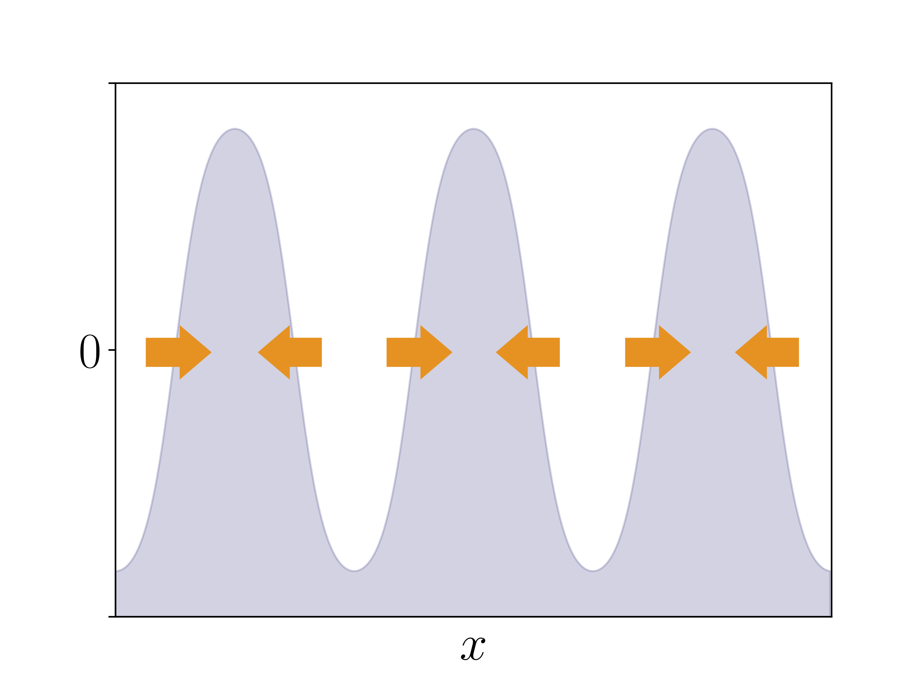
where $\alpha,\beta,\kappa,\alpha^{\prime},\beta^{\prime}$ are positive constants and $c$ can take either sign (the constant terms can be taken to be the same w.l.o.g. as the constant term in $\mu_{\mathrm{B}}$ has no effect on the dynamics) . Observe that when $\beta=\beta^{\prime}$, $\mu_{\mathrm{B}}-\mu_{\mathrm{A}}=(\alpha+\alpha^{\prime})\phi-\kappa\nabla^{2}\phi$, which is linear in $\phi$ with self-adjoint linear operator $Q(\boldsymbol{q})=K(\boldsymbol{q})^{-1}\left[(\alpha+\alpha^{\prime})-\kappa|\boldsymbol{q}|^{2}\right]$. This gives us a continuous parameter $\beta^{\prime}$ that we can tune to bring the system in and out of the equilibrium subspace without dramatically changing the phenomena exhibited. On its own, the Model B sector favours conservative bulk phase separation with the double-well free energy $\mathcal{F}_{\mathrm{B}}=\int\mathrm{d}\boldsymbol{x}\left[-\frac{1}{2}\alpha\phi^{2}+\frac{1}{4}\beta\phi^{4}+\frac{1}{2}\kappa|\boldsymbol{\nabla}\phi|^{2}\right]$, whereas the Model A sector describes non-conservative relaxation towards some fixed target density $\phi_{\mathrm{t}}$. In our previous paper [1], we surveyed the parameter space of this class of models and found two stable stationary solutions: uniform solution and arrested phase separation. The uniform state is observed for small $M_{\mathrm{A}}$, where the local nonconservative relaxations overcome the phase separating diffusive dynamics, fixing the density at the target density $\phi_{\mathrm{t}}$ of the reactions. After crossing over some critical value of $M_{\mathrm{A}}$, the conservative sector dominates and finite domains of alternating phases are formed, as shown in Fig. 1. The length scale of the pattern is determined by the balance of the reactions in the two phases and the steady state current transporting matter across the interface. Interestingly, the information on these macroscopic currents is not available unless we are able to track the Model B and Model A dynamics separately, i.e. distinguishing $\partial_{t}\phi_{\mathrm{A}}$ from $\partial_{t}\phi_{\mathrm{B}}$ in equation (12). This has profound consequences for the entropy production rate as we will see later.

Roughly speaking, $F_{\mathrm{a}}$ ($=F+K\frac{\delta\mathcal{V}}{\delta\phi}$) is the time antisymmetric part of the deterministic evolution; the rigorous version of this statement requires the introduction of the adjoint dynamics. Define the adjoint Fokker-Planck equation such that the time evolution of the probability under the adjoint Fokker-Planck is the same as the forward probability evolution run backwards. Mathematically, this means $\mathcal{P}^{\mathrm{R}}(\tau-t)=\mathcal{P}(t)$, where $\mathcal{P}^{\mathrm{R}}$ is the solution of the adjoint Fokker-Planck equation. Following [18], assume that the adjoint system is also of Langevin type and has the same noise kernel, we want to find the deterministic adjoint dynamics $F^{\mathrm{R}}$.

Starting with the Fokker-Planck equation for the forward probability distribution $\mathcal{P}[\phi,t]$, omitting the dependence on $\phi$ to ease notation,

$$\partial_{t}\mathcal{P}(t)=\delta_{\phi}^{\dagger}(F-\epsilon K\delta_{\phi})\mathcal{P}(t)$$

(23)

where $\delta_{\phi}$ denotes functional derivative with respect to the $\phi$-field, which behaves like a vector. On the other hand, the adjoint Fokker-Planck equation is

$$\partial_{t^{\prime}}\mathcal{P}^{\mathrm{R}}(t^{\prime})=\delta_{\phi}^{\dagger}\left(F^{\mathrm{R}}-\epsilon K\delta_{\phi}\right)\mathcal{P}^{\mathrm{R}}(t^{\prime})$$

(24)

Enforcing the condition that $\mathcal{P}^{\mathrm{R}}(\tau-t)=\mathcal{P}(t)$, we must have $t^{\prime}=\tau-t$ and, by the chain rule, $\partial_{t^{\prime}}P^{\mathrm{R}}(t^{\prime})=-\partial_{t}\mathcal{P}^{\mathrm{R}}(\tau-t)=-\partial_{t}\mathcal{P}(t)$. Substituting into the adjoint Fokker-Planck equation and rearranging the terms into a drift term and noise term, we obtain

$$\partial_{t}\mathcal{P}(t)=\delta_{\phi}^{\dagger}[(2\epsilon K\delta_{\phi}\log(\mathcal{P}(t))-F^{\mathrm{R}})\mathcal{P}(t)-\epsilon K\delta_{\phi}\mathcal{P}(t)]$$

(25)

Comparing the above with equation (23), we can see that the noise terms are the same and the equations will be identical if the drift terms are matched. Recall that $\mathcal{P}\propto\exp(-\epsilon^{-1}\mathcal{V})$, we obtain an expression for $F^{\mathrm{R}}$ in terms of the forward dynamics,

$$F^{\mathrm{R}}(\phi,t)=-2K\delta_{\phi}\mathcal{V}[\phi,t]-F(\phi)$$

(26)

This naturally leads to the definitions of the symmetric and antisymmetric components $F_{\mathrm{s,a}}\equiv(F\pm F^{\mathrm{R}})/2$,

$$F_{\mathrm{s}}=-K\frac{\delta\mathcal{V}}{\delta\phi},\quad F_{\mathrm{a}}=F+K\frac{\delta\mathcal{V}}{\delta\phi}$$

(27)

Note that the forward Fokker-Planck equation needs to be solved to obtain the adjoint dynamics as it requires the value of $\mathcal{V}(t)$ at every instant in time. However, the situation simplifies in steady state where $\mathcal{V}$ remains invariant. Then $F_{\mathrm{s}}$ describes the descent to the minimum of the quasipotential, whereas $F_{\mathrm{a}}$ characterises the excess driving that maintains the system away from equilibrium. It is not surprising that the entropy production in steady state is only a function of $F_{\mathrm{a}}$ – both the entropy production and $F_{\mathrm{a}}$ quantify the amount of time reversal symmetry breaking in the system and vanish in equilibrium.

Our definitions of $F_{\mathrm{s,a}}$ are similar to the symmetric and antisymmetric currents $\boldsymbol{J}_{\mathrm{s,a}}$ in Macroscopic Fluctuation Theory (MFT) [18]. Both rely on the time reversal of the dynamics, but our derivation seeks the time reversal of the probability evolution $\mathcal{P}(t)$, whereas the adjoint dynamics in MFT is defined such that the backward path in the adjoint dynamics has the same probability as the forward path in the forward dynamics. We refer to A for the precise formulae for $\boldsymbol{J}_{\mathrm{s,a}}$ and further discussions on when our adjoint dynamics coincide with that in MFT.

When the principle of detailed balance holds, the probability of observing a path is the same as the probability of observing the reversed path: $\mathbb{R}[\{\boldsymbol{X}\}]=\mathbb{R}[\{\boldsymbol{X}^{\mathrm{R}}\}]$ [23]. So we expect the total entropy production $\Delta S$ of any trajectory to vanish. In addition, the presence of time reversal symmetry means that all equilibrium systems are self-adjoint. Therefore we expect $F=F^{\mathrm{R}}$, $F_{\mathrm{a}}=0$ and the instantaneous entropy production rate $\dot{S}[\phi]$ to be zero for all field configurations $\phi$.

This can be demonstrated more concretely for the relaxational models introduced in section 3. Recall that for this class of systems, $F=-K\frac{\delta\mathcal{F}}{\delta\phi}$ and the stationary measure is the Boltzmann distribution: $\mathcal{V}[\phi]=\mathcal{F}[\phi]$. Thus, for a $(\phi,\partial_{t}\phi)_{t\in[0,\tau]}$ trajectory, the internal and external entropy productions in steady state (equilibrium) are,

$$\eqalign{\quad\Delta S_{\mathrm{Int}}&=\frac{1}{\epsilon}\left(\mathcal{F}[\phi(\tau)]-\mathcal{F}[\phi(0)]\right)\\ \quad\Delta S_{\mathrm{Ext}}&=-\frac{1}{\epsilon}\int\mathrm{d}t\,\partial_{t}\phi^{\dagger}\mu=-\frac{1}{\epsilon}\int\mathrm{d}t\,\partial_{t}\phi^{\dagger}\frac{\delta\mathcal{F}}{\delta\phi}=-\frac{1}{\epsilon}\left(\mathcal{F}[\phi(\tau)]-\mathcal{F}[\phi(0)]\right)}$$

(28)

Observe that the two parts cancel out exactly. The total entropy production $\Delta S$ vanishes for each trajectory – the entropy has merely been transferred from the system to the surroundings but the overall value remains the same.

As a consistency check, we can also compute the instantaneous entropy production rate $\dot{S}$ via equation (21). Recall from equation (27) that $F_{\mathrm{a}}=F+K\frac{\delta\mathcal{V}}{\delta\phi}$, which is identically zero in equilibrium since $\mathcal{V}_{\mathrm{ss}}=\mathcal{F}$. The steady state EPR $\dot{S}_{\mathrm{ss}}$ and its local decomposition $\dot{s}$ are only functions of $F_{\mathrm{a}}$ but not $F_{\mathrm{s}}$, hence must both vanish, as expected of time-symmetric dynamics.

Having checked that the entropy production indeed vanishes in equilibrium, we proceed to probe the class of non-equilibrium diffusive systems introduced in section 3.1 that breaks time reversal symmetry in a ‘minimal’ way by adding a driving term to Model B. We will compute the steady state entropy production rate $\dot{S}_{\mathrm{ss}}$ and its non-negative local decomposition $\dot{s}(\boldsymbol{x})$, followed by a discussion of their physical interpretations. For convenience, throughout this section we will omit the subscript ‘B’ as we only discuss mass-conserving systems.

Recall from section 3.1 that the noise kernel $K$ for mass-conserving systems is $-M\nabla^{2}$, from which we can straight forwardly deduce the antisymmetric component $F_{\mathrm{a}}$ and a formal expression for $\dot{S}_{\mathrm{ss}}$

$$\eqalign{F_{\mathrm{a}}&=F+K\delta_{\phi}\mathcal{V}_{\mathrm{ss}}=M\boldsymbol{\nabla}\cdot\left[\boldsymbol{\nabla}\left(\mu-\delta_{\phi}\mathcal{V}_{\mathrm{ss}}\right)-\boldsymbol{E}\right]\\ \dot{S}_{\mathrm{ss}}&=\frac{1}{\epsilon M}\int\mathrm{d}\boldsymbol{x}\,F_{\mathrm{a}}(\boldsymbol{x})(\nabla^{-2}F_{\mathrm{a}})(\boldsymbol{x})}$$

(29)

The inverse of the Laplacian operator, denoted as $\nabla^{-2}$, is well defined up to a constant once the boundary conditions are specified. In fact, we can infer that the constant piece must be zero because both $\mathcal{V}$ and $\mathbb{A}$ have no contribution from the $\boldsymbol{q}=0$ mode due to mass conservation, meaning that the entropy production rate cannot have a zero-mode contribution either.

The integral in the expression for $\dot{S}_{\mathrm{ss}}$ gives one spatial decomposition, but that is not the non-negative local EPR $\dot{s}(\boldsymbol{x})$. Recall that $\dot{s}(\boldsymbol{x})=\epsilon^{-1}|Y(\boldsymbol{x})|^{2}$, where $|Y|=|\sigma^{-1}F_{\mathrm{a}}|$ and $\sigma(\boldsymbol{q})=-i\sqrt{M}|\boldsymbol{q}|$. The subtleties with $\sigma(\boldsymbol{q}=0)=0$ can again be mitigated by realising that there cannot be a $\boldsymbol{q}=0$ mode in the entropy production rate. For mass-conserving systems, as alluded to in section 4.1 and discussed in A, $F_{\mathrm{a}}$ is closely related to the antisymmetric current $\boldsymbol{J}_{\mathrm{a}}=-\boldsymbol{\nabla}\left(\mu-\delta_{\phi}\mathcal{V}_{\mathrm{ss}}\right)+\boldsymbol{E}$ in Macroscopic Fluctuation Theory. In fact, $F_{\mathrm{a}}=-\boldsymbol{\nabla}\boldsymbol{\cdot}\boldsymbol{J}_{\mathrm{a}}$, which in Fourier space translates to $F_{\mathrm{a}}(\boldsymbol{q})=i\boldsymbol{q}\boldsymbol{\cdot}\boldsymbol{J}_{\mathrm{a}}(\boldsymbol{q})$, implying that we can choose $Y(\boldsymbol{q})=M^{-1/2}\hat{\boldsymbol{q}}\boldsymbol{\cdot}\boldsymbol{J}_{\mathrm{a}}$, where $\hat{\boldsymbol{q}}=\boldsymbol{q}/|\boldsymbol{q}|$, with the additional condition that $Y(\boldsymbol{q}=0)=0$. The physical interpretation of this becomes clearer if we decompose $\boldsymbol{J}_{\mathrm{a}}$ into a pure gradient piece and a pure curl piece,

$$\boldsymbol{J}_{\mathrm{a}}=\boldsymbol{\nabla}\Phi+\boldsymbol{\nabla}\times A$$

(30)

where $\Phi$ is a scalar field and $A$ is a vector field. This is the Helmholtz decomposition, which can always be performed for any vector field: $\Phi=\nabla^{-2}\boldsymbol{\nabla}\boldsymbol{\cdot}\boldsymbol{J}_{\mathrm{a}}$, where the inverse Laplacian is well defined as described above. Let the pure gradient part be $\widetilde{\boldsymbol{J}}_{\mathrm{a}}=\boldsymbol{\nabla}\Phi$. Since $\widetilde{\boldsymbol{J}}_{\mathrm{a}}(\boldsymbol{q})=-i\boldsymbol{q}\Phi(\boldsymbol{q})$, $\widetilde{\boldsymbol{J}}_{\mathrm{a}}$ is in the direction of $\boldsymbol{q}$ while $(\boldsymbol{\nabla}\times\boldsymbol{A})(\boldsymbol{q})=-i\boldsymbol{q}\times\boldsymbol{A}(\boldsymbol{q})$ is perpendicular to $\boldsymbol{q}$. Therefore

$$|Y(\boldsymbol{q})|=M^{-1/2}|\hat{\boldsymbol{q}}\boldsymbol{\cdot}\boldsymbol{J}_{\mathrm{a}}(\boldsymbol{q})|=M^{-1/2}|\widetilde{\boldsymbol{J}}_{\mathrm{a}}(\boldsymbol{q})|$$

(31)

Fourier transform back to real space,

$$\dot{s}(\boldsymbol{x})=\epsilon^{-1}|Y(\boldsymbol{x})|^{2}=(\epsilon M)^{-1}\widetilde{\boldsymbol{J}}_{\mathrm{a}}(\boldsymbol{x})\cdot\widetilde{\boldsymbol{J}}_{\mathrm{a}}(\boldsymbol{x})$$

(32)

In other words, any curl piece (including any constant as this cannot be written as a gradient) in the current gives no contribution to the entropy production rate, which makes sense as the non-gradient part of the current has no effect on the $(\phi,\partial_{t}\phi)$ trajectories either.

Recall the simple exactly solvable example of particles driven around a 1D ring by a constant force $\boldsymbol{\gamma}$, as discussed in section 3. In this case, the steady state probabilities are independent of the driving (i.e. $\mathcal{V}_{\mathrm{ss}}=\mathcal{F}$), leading to a clear decomposition of the symmetric and antisymmetric dynamics

$$F_{\mathrm{s}}=M\partial_{x}^{2}\mu,\quad F_{\mathrm{a}}=-M\gamma\partial_{x}\phi$$

(33)

The symmetric part controls the descent down the free energy gradient while the antisymmetric part drives the system around the ring. In 1D, the only curl contribution in $J_{\mathrm{a}}$ is the constant piece, which we need to subtract off: $\widetilde{J}_{\mathrm{a}}(x)=M\gamma(\phi(x)-\bar{\phi})$, where $\bar{\phi}$ is the mean density. Therefore the local entropy production is

$$\dot{s}(x)=\epsilon^{-1}M|\boldsymbol{\gamma}|^{2}\left(\phi(x)-\bar{\phi}\right)^{2}$$

(34)

For more complicated driving, such as Active Model B+, the quasipotential $\mathcal{V}$ is often unknown so it is usually not possible compute the entropy production exactly.

Similarly, for Model AB, there is no known solution for the full stochastic dynamics. Nevertheless, one can still write down an expression for the steady state entropy production, assuming that $\mathcal{V}_{\mathrm{ss}}$ can at least be approximated. Recall the definition of Model AB from equation (14): $\partial_{t}\phi=M_{\mathrm{B}}\nabla^{2}\mu_{\mathrm{B}}-M_{\mathrm{A}}\mu_{\mathrm{A}}+\sqrt{2\epsilon}\sigma\Lambda$ where $\sigma(\boldsymbol{q})=\sqrt{M_{\mathrm{A}}}-i|\boldsymbol{q}|\sqrt{M_{\mathrm{B}}}$. The antisymmetric component in steady state is

$$F_{\mathrm{a}}=M_{\mathrm{B}}\nabla^{2}\left(\mu_{\mathrm{B}}-\frac{\delta\mathcal{V}_{\mathrm{ss}}}{\delta\phi}\right)-M_{\mathrm{A}}\left(\mu_{\mathrm{A}}-\frac{\delta\mathcal{V}_{\mathrm{ss}}}{\delta\phi}\right)$$

(35)

where as before $\mathcal{V}_{\mathrm{ss}}$ is the (unknown) steady state quasipotential. Recall that the local decomposition $\dot{s}(\boldsymbol{x})=\epsilon^{-1}Y^{2}$ where $|Y|=|\sigma^{-1}F_{\mathrm{a}}|$. Since $\sigma$ is invertible and diagonal in Fourier space, given $\mathcal{V}_{\mathrm{ss}}$, $Y$ can be computed independently for each mode: $|Y(\boldsymbol{q})|=|F_{\mathrm{a}}(\boldsymbol{q})/\sigma(\boldsymbol{q})|$. It is possible to then Fourier transform back to real space to obtain an expression for $\dot{s}(\boldsymbol{x})$, but we will not write it out explicitly here as it’s both complicated and not particularly enlightening.

As we have shown with examples, in general it is extremely rare that one can find an exact analytical expressions for $\dot{S}_{\mathrm{ss}}$ or its local decomposition $\dot{s}(\boldsymbol{x})$, as they require the knowledge of $F_{\mathrm{a}}$ which in turn depends on an exact solution for the steady state probability distribution (recall that $F_{\mathrm{a}}=F+K\frac{\delta\mathcal{V}}{\delta\phi}$ and $\mathcal{P}_{\mathrm{ss}}=\exp(-\epsilon^{-1}\mathcal{V}_{\mathrm{ss}})$). However, when the noise strength $\epsilon$ is small, the stationary distribution is approximately a Gaussian distribution around the deterministic steady state as we will see shortly³³ 3 In cases where the quasipotential has multiple minima, the approximation is valid for the time window before the escape time of the local minimum. . As a result, the steady state EPR can be approximated in the small $\epsilon$ limit.

The small noise approximation is a standard method for stochastic processes: first expand the scalar field $\phi=\phi_{0}+\sqrt{\epsilon}\phi_{1}+O(\epsilon)$, then substitute into equation (8) and equate the terms to order $\epsilon^{0}$ and $\epsilon^{1/2}$ separately [22, 37],

$$\eqalign{\partial_{t}\phi_{0}&=F(\phi_{0})\\ \partial_{t}\phi_{1}&=A(\phi_{0})\phi_{1}+\sqrt{2}\sigma\Lambda}$$

(36)

Here $A(\phi_{0})$ is the Jacobian “matrix” defined as $A_{ij}(\phi_{0})\equiv\delta_{\phi_{j}}F_{i}|_{\phi=\phi_{0}}$. Note that $A$ is a function of $\phi_{0}$ but not $\phi_{1}$. The zeroth order field $\phi_{0}$ captures the deterministic evolution while the $\phi_{1}$ equation corresponds to the Gaussian fluctuation around the deterministic trajectory. Once $\phi_{0}$ has reached its stationary value $\phi_{0}^{\mathrm{ss}}$, the Jacobian $A$ must be negative definite (all eigenvalues negative)⁴⁴ 4 Modulo any Goldstone mode – see C. This means $\phi_{1}$ decays exponentially towards a steady state with mean value zero. The steady state correlation of $\phi_{1}$, defined as $C=\left\langle\phi_{1}\phi_{1}^{\dagger}\right\rangle$, can be calculated using the Lyapunov equation [22, 37],

$$AC+CA^{\dagger}=-2K$$

(37)

Once $C$ is known, the steady state quasipotential $\mathcal{V}_{\mathrm{ss}}$ can also be obtained to lowest order in $\epsilon$. As $\phi_{0}$ is entirely deterministic, the quasipotential is only a function of the fluctuating field $\phi_{1}$,

$$\mathcal{V}_{\mathrm{ss}}[\phi_{1}]=\frac{\epsilon}{2}\phi_{1}^{\dagger}G\phi_{1}+O(\epsilon^{3/2})$$

(38)

where $G$ is the inverse of $C$. This holds provided that the system has no continuous symmetry (e.g. translation symmetry if periodic boundary conditions are used); otherwise the additional degree of symmetry has to be explicitly projected out as shown in C so that $G=C^{-1}$ in the subspace without the Goldstone mode. Now we have all the pieces to calculate the time-antisymmetric component $F_{\mathrm{a}}$ and $Y=\sigma^{-1}F_{\mathrm{a}}$,

$$\eqalign{F_{\mathrm{a}}&=F(\phi)+K\frac{\delta\mathcal{V}_{\mathrm{ss}}}{\delta\phi}=\sqrt{\epsilon}(A+KG)\phi_{1}+O(\epsilon)\\ Y&=\sqrt{\epsilon}\left(\sigma^{-1}A+\sigma^{\dagger}G\right)\phi_{1}+O(\epsilon)}$$

(39)

For convenience, define the matrix $E=\sigma^{-1}A+\sigma^{\dagger}G$ such that $Y=\sqrt{\epsilon}E\phi_{1}+O(\epsilon)$. Notice that both $F_{\mathrm{a}}$ and $Y$ are $O(\sqrt{\epsilon})$, implying that they vanish at the deterministic order and only depend on the fluctuations. Finally, we can write down the local entropy production rate for a steady state configuration $\phi=\phi_{0}+\sqrt{\epsilon}\phi_{1}+O(\epsilon)$,

$$\dot{s}(\boldsymbol{x})[\phi_{1}]=\epsilon^{-1}Y(\boldsymbol{x})^{2}=\int\mathrm{d}\boldsymbol{y}\mathrm{d}\boldsymbol{z}E(\boldsymbol{x},\boldsymbol{y})\phi_{1}(\boldsymbol{y})E(\boldsymbol{x},\boldsymbol{z})\phi_{1}(\boldsymbol{z})+h.o.t.$$

(40)

where $h.o.t.$ stands for ‘higher order terms’. We can proceed to average over the steady state distribution for $\phi_{1}$ to obtain the ensemble EPR,

$$\eqalign{\left\langle\dot{s}(\boldsymbol{x})\right\rangle&=\int\mathrm{d}\boldsymbol{y}\mathrm{d}\boldsymbol{z}E(\boldsymbol{x},\boldsymbol{y})C(\boldsymbol{y},\boldsymbol{z})E^{\dagger}(\boldsymbol{z},\boldsymbol{x})+h.o.t.\\ &=\mathrm{Diag}[ECE^{\dagger}](\boldsymbol{x})+h.o.t.}$$

(41)

where “Diag” denotes the diagonal of a matrix. It is worth noting that we also get $\left\langle\dot{S}_{\mathrm{ss}}[\phi]\right\rangle$ for free: $\left\langle\dot{S}_{\mathrm{ss}}\right\rangle=\int\mathrm{d}\boldsymbol{x}\left\langle\dot{s}(\boldsymbol{x})\right\rangle=\mathrm{Tr}(ECE^{\dagger})+h.o.t.$ Thus far, we have arrived at a general expression for the lowest order noise expansion for the steady state EPR of any scalar Langevin system. The only knowledge required for this calculation is the deterministic steady state solution, which is both more analytically tractable and less numerically expensive than solving the stochastic dynamics.

Bibliography

- [1] Y. I. Li and M. E. Cates. Non-equilibrium phase separation with reactions: a canonical model and its behaviour. J. Stat. Mech.: Theory Exp., 2020(5):053206, 2020.
- [2] M. E Cates and J. Tailleur. Motility-induced phase separation. Annu. Rev. Condens. Matter Phys., 6:219–244, 2015.
- [3] S. Ramaswamy. The mechanics and statistics of active matter. Annual Review of Condensed Matter Physics, 1(1):323–345, 2010.
- [4] M. C. Marchetti, J.-F. Joanny, S. Ramaswamy, T. B. Liverpool, J. Prost, M. Rao, and R. A. Simha. Hydrodynamics of soft active matter. Rev. Mod. Phys., 85:1143, 2013.
- [5] B. Schmittmann and R. K. P. Zia. Statistical mechanics of driven diffusive systems, volume 17 of Phase Transitions and Critical Phenomena. Academic Press, 1995.
- [6] M. R. Evans, Y. Kafri, H. M. Koduvely, and D. Mukamel. Phase separation and coarsening in one-dimensional driven diffusive systems: local dynamics leading to long-range Hamiltonians. Phys. Rev. E, 58(3):2764, 1998.
- [7] É. Fodor, C. Nardini, M. E. Cates, J. Tailleur, P. Visco, and F. van Wijland. How far from equilibrium is active matter? Phys. Rev. Lett., 117:038103, 2016.
- [8] C. Nardini, É. Fodor, E. Tjhung, F. van Wijland, J. Tailleur, and M. E. Cates. Entropy production in field theories without time-reversal symmetry: Quantifying the non-equilibrium character of active matter. Phys. Rev. X, 7:021007, 2017.
- [9] U. Seifert. Stochastic thermodynamics, fluctuation theorems and molecular machines. Rep. Prog. Phys., 75:126001, 2012.
- [10] P. Pietzonka and U. Seifert. Entropy production of active particles and for particles in active baths. J. Phys. A, 51:01LT01, 2017.
- [11] U. Seifert. Entropy production along a stochastic trajectory and an integral fluctuation theorem. Phys. Rev. Lett, 95:040602, 2005.
- [12] D. Mandal, K. Klymko, and M. R. DeWeese. Entropy production and fluctuation theorems for active matter. Phys. Rev. Lett., 119:258001, 2017.
- [13] S. Shankar and M. C. Marchetti. Hidden entropy production and work fluctuations in an ideal active gas. Phys. Rev. E, 98:020604, 2018.
- [14] O. Niggemann and U. Seifert. Field-theoretic thermodynamic uncertainty relation. J. Stat. Phys., pages 1–33, 2020.
- [15] L. Dabelow, S. Bo, and R. Eichhorn. Irreversibility in active matter systems: Fluctuation theorem and mutual information. Phys. Rev. X, 9:021009, 2019.
- [16] E. Tjhung, C. Nardini, and M. E. Cates. Cluster phases and bubbly phase separation in active fluids: Reversal of the ostwald process. Phys. Rev. X, 8:031080, 2018.
- [17] P. C. Hohenberg and B. I. Halperin. Theory of dynamic critical phenomena. Rev. Mod. Phys., 49:435–479, 1977.
- [18] L. Bertini, A. De Sole, D. Gabrielli, G. Jona-Lasinio, and C. Landim. Macroscopic fluctuation theory. Rev. Mod. Phys., 87:593, 2015.
- [19] A. W. C. Lau and T. C. Lubensky. State-dependent diffusion: Thermodynamic consistency and its path integral formulation. Phys. Rev. E, 76:011123, 2007.
- [20] T. Markovich, É. Fodor, E. Tjhung, and M. E. Cates. Thermodynamics of active field theories: Energetic cost of coupling to reservoirs. 2020.
- [21] U. C. Täuber. Critical Dynamics: a Field Theory Approach to Equilibrium and Non-equilibrium Scaling Behavior. Cambridge University Press, 2014.
- [22] C. Gardiner. Stochastic Methods, volume 4. Springer Berlin, 2009.
- [23] D. Mukamel. Phase transitions in nonequilibrium systems. In M.E. Cates and M.R. Evans, editors, Soft and fragile matter, Scottish Graduate Series, page 237. Taylor & Francis, 2000.
- [24] P. M. Chaikin, T. C. Lubensky, and T. A. Witten. Principles of Condensed Matter Physics, volume 10. Cambridge University Press, 1995.
- [25] M. E. Cates. Active field theories. arXiv preprint arXiv:1904.01330, 2019.
- [26] J. Toner and Y. Tu. Long-range order in a two-dimensional dynamical XY model: how birds fly together. Phys. Rev. Lett., 75:4326, 1995.
- [27] C. A. Weber, D. Zwicker, F. Jülicher, and C. F. Lee. Physics of active emulsions. Rep. Prog. Phys., 82:064601, 2019.
- [28] T. Grafke, M. E. Cates, and E. Vanden-Eijnden. Spatiotemporal self-organization of fluctuating bacterial colonies. Phys. Rev. Lett., 119:188003, 2017.
- [29] M. E. Cates, D. Marenduzzo, I. Pagonabarraga, and J. Tailleur. Arrested phase separation in reproducing bacteria creates a generic route to pattern formation. Proc. Natl. Acad. Sci. U.S.A., 107:11715–11720, 2010.
- [30] S. C. Glotzer, D. Stauffer, and N. Jan. Monte carlo simulations of phase separation in chemically reactive binary mixtures. Phys. Rev. Lett., 72:4109–4112, 1994.
- [31] S. C. Glotzer, E. A. Di Marzio, and M. Muthukumar. Reaction-controlled morphology of phase-separating mixtures. Phys. Rev. Lett., 74:2034–2037, 1995.
- [32] S. C. Glotzer and A. Coniglio. Self-consistent solution of phase separation with competing interactions. Phys. Rev. E, 50:4241–4244, 1994.
- [33] D Zwicker, R Seyboldt, C. A Weber, A. A Hyman, and F Jülicher. Growth and division of active droplets provides a model for protocells. Nat. Phys., 13:408, 2017.
- [34] D. Zwicker, A. A. Hyman, and F. Jülicher. Suppression of ostwald ripening in active emulsions. Phys. Rev. E, 92:012317, 2015.
- [35] S. Puri and H. L. Frisch. Phase separation in binary mixtures with chemical reactions. Int. J. Mod. Phys. B, 12:1623–1641, 1998.
- [36] L. Onsager and S. Machlup. Fluctuations and irreversible processes. Phys. Rev., 91:1505, 1953.
- [37] N. G. van Kampen. Stochastic Processes in Physics and Chemistry, volume 1. Elsevier, 1992.
- [38] A. Borthne and R. Adhikari. Fluctuations, response, and self-sustained oscillations in an active cosserat solid. To appear.
- [39] R. H. Bartels and G. W. Stewart. Solution of the matrix equation AX + XB = C. Commun. ACM, 15:820–826, 1972.