Review: Deep Learning in Electron Microscopy
Abstract
Deep learning is transforming most areas of science and technology, including electron microscopy. This review paper offers a practical perspective aimed at developers with limited familiarity. For context, we review popular applications of deep learning in electron microscopy. Afterwards, we discuss hardware and software needed to get started with deep learning and interface with electron microscopes. We then review neural network components, popular architectures, and their optimization. Finally, we discuss future directions of deep learning in electron microscopy.
Keywords: deep learning, electron microscopy, review.
1 Introduction
Following decades of exponential increases in computational capability[1] and widespread data availability[2, 3], scientists can routinely develop artificial neural networks[4, 5, 6, 7, 8, 9, 10, 11] (ANNs) to enable new science and technology[12, 13, 14, 15, 16, 17]. The resulting deep learning revolution[18, 19] has enabled superhuman performance in image classification[20, 21, 22, 23], games[24, 25, 26, 27, 28, 29], medical analysis[30, 31], relational reasoning[32], speech recognition[33, 34] and many other applications[35, 36]. This introduction focuses on deep learning in electron microscopy and is aimed at developers with limited familiarity. For context, we therefore review popular applications of deep learning in electron microscopy. We then review resources available to support researchers and outline electron microscopy. Finally, we review popular ANN architectures and their optimization, or “training”, and discuss future trends in artificial intelligence (AI) for electron microscopy.
Deep learning is motivated by universal approximator theorems[37, 38, 39, 40, 41, 42, 43, 44, 45], which state that sufficiently deep and wide[37, 46, 40] ANNs can approximate functions to arbitrary accuracy. It follows that ANNs can always match or surpass the performance of methods crafted by humans. In practice, deep neural networks (DNNs) reliably[47] learn to express[48, 49, 50, 51] generalizable[52, 53, 54, 55, 56, 57, 58, 59] models without a prior understanding of physics. As a result, deep learning is freeing physicists from a need to devise equations to model complicated phenomena[60, 61, 13, 14, 16]. Many modern ANNs have millions of parameters, so inference often takes tens of milliseconds on graphical processing units (GPUs) or other hardware accelerators[62]. It is therefore unusual to develop ANNs to approximate computationally efficient methods with exact solutions, such as the fast Fourier transform[63, 64, 65] (FFT). However, ANNs are able to leverage an understanding of physics to accelerate time-consuming or iterative calculations[66, 67, 68, 69], improve accuracy of methods[70, 30, 31], and find solutions that are otherwise intractable[24, 71].

1.1 Improving Signal-to-Noise
A popular application of deep learning is to improve signal-to-noise[74, 75]. For example, of medical electrical[76, 77], medical image[78, 79, 80], optical microscopy[81, 82, 83, 84], and speech[85, 86, 87, 88] signals. There are many traditional denoising algorithms that are not based on deep learning[89, 90, 91], including linear[92, 93] and non-linear[94, 95, 96, 97, 98, 99, 100, 101, 102] spatial domain filters, Wiener[103, 104, 105] filters, non-linear[106, 107, 108, 109, 110, 111] wavelet domain filters, curvelet transforms[112, 113], contourlet transforms[114, 115], hybrid algorithms[116, 117, 118, 119, 120, 121, 122] that operate in both spatial and transformed domains, and dictionary-based learning[123, 124, 125, 126, 127]. However, traditional denoising algorithms are limited by features (often laboriously) crafted by humans and cannot exploit domain-specific context. In perspective, they leverage an ever-increasingly accurate representation of physics to denoise signals. However, traditional algorithms are limited by the difficulty of programmatically describing a complicated reality. As a case in point, an ANN was able to outperform decades of advances in traditional denoising algorithms after training on two GPUs for a week[70].
Definitions of electron microscope noise can include statistical noise[128, 129, 130, 131, 132, 133, 134, 135], aberrations[136], scan distortions[137, 138, 139, 140], specimen drift[141], and electron beam damage[142]. Statistical noise is often minimized by either increasing electron dose or applying traditional denoising algorithms[143, 144]. There are a variety of denoising algorithms developed for electron microscopy, including algorithms based on block matching[145], contourlet transforms[114, 115], energy minimization[146], fast patch reorderings[147], Gaussian kernel density estimation[148], Kronecker envelope principal component analysis[149] (PCA), non-local means and Zernike moments[150], singular value thresholding[151], wavelets[152], and other approaches[153, 154, 141, 155, 156]. Noise that is not statistical is often minimized by hardware. For example, by using aberration correctors[136, 157, 158, 159], choosing scanning transmission electron microscopy (STEM) scan shapes and speeds that minimize distortions[138], and using stable sample holders to reduce drift[160]. Beam damage can also be reduced by using minimal electron voltage and electron dose[161, 162, 163], or dose-fractionation across multiple frames in multi-pass transmission electron microscopy[164, 165, 166] (TEM) or STEM[167].
Deep learning is being applied to improve signal-to-noise for a variety of applications[168, 169, 170, 171, 172, 173, 174, 175, 176]. Most approaches in electron microscopy involve training ANNs to either map low-quality experimental[177], artificially deteriorated[70, 178] or synthetic[179, 180, 181, 182] inputs to paired high-quality experimental measurements. For example, applications of a DNN trained with artificially deteriorated TEM images are shown in figure 1. However, ANNs have also been trained with unpaired datasets of low-quality and high-quality electron micrographs[183], or pairs of low-quality electron micrographs[184, 185]. Another approach is Noise2Void[168], ANNs are trained from single noisy images. However, Noise2Void removes information by masking noisy input pixels corresponding to target output pixels. So far, most ANNs that improve electron microscope signal-to-noise have been trained to decrease statistical noise[183, 177, 70, 186, 181, 182, 184, 179, 180, 181] as other approaches have been developed to correct electron microscope scan distortions[187, 188] and specimen drift[189, 188, 141]. However, we anticipate that ANNs will be developed to correct a variety of electron microscopy noise as ANNs have been developed for aberration correction of optical microscopy[190, 191, 192, 193, 194, 195] and photoacoustic[196] signals.

1.2 Compressed Sensing
Compressed sensing[203, 204, 205, 206, 207] is the efficient reconstruction of a signal from a subset of measurements. Applications include faster medical imaging[208, 209, 210], image compression[211, 212], increasing image resolution[213, 214], lower medical radiation exposure[215, 216, 217], and low-light vision[218, 219]. In STEM, compressed sensing has enabled electron beam exposure and scan time to be decreased by 10-100 with minimal information loss[201, 202]. Thus, compressed sensing can be essential to investigations where the high current density of electron probes damages specimens[161, 220, 221, 222, 223, 224, 225, 226]. Even if the effects of beam damage can be corrected by postprocessing, the damage to specimens is often permanent. Examples of beam-sensitive materials include organic crystals[227], metal-organic frameworks[228], nanotubes[229], and nanoparticle dispersions[230]. In electron microscopy, compressed sensing is especially effective due to high signal redundancy[231]. For example, most electron microscopy images are sampled at 5-10 their Nyquist rates[232] to ease visual inspection, decrease sub-Nyquist aliasing[233], and avoid undersampling.
Perhaps the most popular approach to compressed sensing is upsampling or infilling a uniformly spaced grid of signals[234, 235, 236]. Interpolation methods include Lancsoz[234], nearest neighbour[237], polynomial interpolation[238], Wiener[239] and other resampling methods[240, 241, 242]. However, a variety of other strategies to minimize STEM beam damage have also been proposed, including dose fractionation[243] and a variety of sparse data collection methods[244]. Perhaps the most intensively investigated approach to the latter is sampling a random subset of pixels, followed by reconstruction using an inpainting algorithm[245, 244, 246, 247, 248, 249]. Random sampling of pixels is nearly optimal for reconstruction by compressed sensing algorithms[250]. However, random sampling exceeds the design parameters of standard electron beam deflection systems, and can only be performed by collecting data slowly[251, 138], or with the addition of a fast deflection or blanking system[247, 252].
Sparse data collection methods that are more compatible with conventional STEM electron beam deflection systems have also been investigated. For example, maintaining a linear fast scan deflection whilst using a widely-spaced slow scan axis with some small random ‘jitter’[251, 245]. However, even small jumps in electron beam position can lead to a significant difference between nominal and actual beam positions in a fast scan. Such jumps can be avoided by driving functions with continuous derivatives, such as those for spiral and Lissajous scan paths[201, 253, 138, 254, 247]. Sang[138, 254] considered a variety of scans including Archimedes and Fermat spirals, and scans with constant angular or linear displacements, by driving electron beam deflectors with a field-programmable gate array[255] (FPGA) based system[138]. Spirals with constant angular velocity place the least demand on electron beam deflectors. However, dwell times, and therefore electron dose, decreases with radius. Conversely, spirals created with constant spatial speeds are prone to systematic image distortions due to lags in deflector responses. In practice, fixed doses are preferable as they simplify visual inspection and limit the dose dependence of STEM noise[129].
Deep learning can leverage an understanding of physics to infill images[256, 257, 258]. Example applications include increasing scanning electron microscopy[259, 178, 260] (SEM), STEM[202, 261] and TEM[262] resolution, and infilling continuous sparse scans[201]. Example applications of DNNs to complete sparse spiral and grid scans are shown in figure 2. However, caution should be used when infilling large regions as ANNs may generate artefacts if a signal is unpredictable[201]. A popular alternative to deep learning for infilling large regions is exemplar-based infilling[263, 264, 265, 266]. However, exemplar-based infilling often leaves artefacts[267] and is usually limited to leveraging information from single images. Smaller regions are often infilled by fast marching[268], Navier-Stokes infilling[269], or interpolation[238].
1.3 Labelling
Deep learning has been the basis of state-of-the-art classification[270, 271, 272, 273] since convolutional neural networks (CNNs) enabled a breakthrough in classification accuracy on ImageNet[71]. Most classifiers are single feedforward neural networks (FNNs) that learn to predict discrete labels. In electron microscopy, applications include classifying image region quality[274, 275], material structures[276, 277], and image resolution[278]. However, siamese[279, 280, 281] and dynamically parameterized[282] networks can more quickly learn to recognise images. Finally, labelling ANNs can learn to predict continuous features, such as mechanical properties[283]. Labelling ANNs are often combined with other methods. For example, ANNs can be used to automatically identify particle locations[284, 285, 186, 286] to ease subsequent processing.

1.4 Semantic Segmentation
Semantic segmentation is the classification of pixels into discrete categories. In electron microscopy, applications include the automatic identification of local features[288, 289], such as defects[290, 291], dopants[292], material phases[293], material structures[294, 295], dynamic surface phenomena[296], and chemical phases in nanoparticles[297]. Early approaches to semantic segmentation used simple rules. However, such methods were not robust to a high variety of data[298]. Subsequently, more adaptive algorithms based on soft-computing[299] and fuzzy algorithms[300] were developed to use geometric shapes as priors. However, these methods were limited by programmed features and struggled to handle the high variety of data.
To improve performance, DNNs have been trained to semantically segment images[301, 302, 303, 304, 305, 306, 307, 308]. Semantic segmentation DNNs have been developed for focused ion beam scanning electron microscopy[309, 310, 311] (FIB-SEM), SEM[312, 313, 314, 311], STEM[315, 287], and TEM[286, 316, 317, 310, 318, 311, 319]. For example, applications of a DNN to semantic segmentation of STEM images of steel are shown in figure 3. Deep learning based semantic segmentation also has a high variety of applications outside of electron microscopy, including autonomous driving[320, 321, 322, 323, 324], dietary monitoring[325, 326], magnetic resonance images[327, 328, 329, 330, 331], medical images[332, 333, 334] such as prenatal ultrasound[335, 336, 337, 338], and satellite image translation[339, 340, 341, 342, 343]. Most DNNs for semantic segmentation are trained with images segmented by humans. However, human labelling may be too expensive, time-consuming, or inappropriate for sensitive data. Unsupervised semantic segmentation can avoid these difficulties by learning to segment images from an additional dataset of segmented images[344] or image-level labels[345, 346, 347, 348]. However, unsupervised semantic segmentation networks are often less accurate than supervised networks.
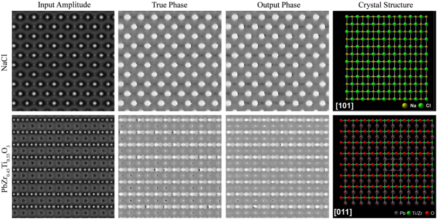
1.5 Exit Wavefunction Reconstruction
Electrons exhibit wave-particle duality[350, 351], so electron propagation is often described by wave optics[352]. Applications of electron wavefunctions exiting materials[353] include determining projected potentials and corresponding crystal structure information[354, 355], information storage, point spread function deconvolution, improving contrast, aberration correction[356], thickness measurement[357], and electric and magnetic structure determination[358, 359]. Usually, exit wavefunctions are either iteratively reconstructed from focal series[360, 361, 362, 363, 364] or recorded by electron holography[352, 363, 365]. However, iterative reconstruction is often too slow for live applications, and holography is sensitive to distortions and may require expensive microscope modification.
Non-iterative methods based on DNNs have been developed to reconstruct optical exit wavefunctions from focal series[69] or single images[366, 367, 368]. Subsequently, DNNs have been developed to reconstruct exit wavefunctions from single TEM images[349], as shown in figure 4. Indeed, deep learning is increasingly being applied to accelerated quantum mechanics[369, 370, 371, 372, 373, 374]. Other examples of DNNs adding new dimensions to data include semantic segmentation described in section 1.4, and reconstructing 3D atomic distortions from 2D images[375]. Non-iterative methods that do not use ANNs to recover phase information from single images have also been developed[376, 377]. However, they are limited to defocused images in the Fresnel regime[376], or to non-planar incident wavefunctions in the Fraunhofer regime[377].
2 Resources
Access to scientific resources is essential to scientific enterprise[378]. Fortunately, most resources needed to get started with machine learning are freely available. This section provides directions to various machine learning resources, including how to access deep learning frameworks, a free GPU or tensor processing unit (TPU) to accelerate tensor computations, platforms that host datasets and source code, and pretrained models. To support the ideals of open science embodied by Plan S[379, 378, 380], we focus on resources that enhance collaboration and enable open access[381]. We also discuss how electron microscopes can interface with ANNs and the importance of machine learning resources in the context of electron microscopy. However, we expect that our insights into electron microscopy can be generalized to other scientific fields.
2.1 Hardware Acceleration
A DNN is an ANN with multiple layers that perform a sequence of tensor operations. Tensors can either be computed on central processing units (CPUs) or hardware accelerators[62], such as FPGAs[382, 383, 384, 385], GPUs[386, 387, 388], and TPUs[389, 390, 391]. Most benchmarks indicate that GPUs and TPUs outperform CPUs for typical DNNs that could be used for image processing[392, 393, 394, 395, 396] in electron microscopy. However, GPU and CPU performance can be comparable when CPU computation is optimized[397]. TPUs often outperform GPUs[394], and FPGAs can outperform GPUs[398, 399] if FPGAs have sufficient arithmetic units[400, 401]. Typical power consumption per TFLOPS[402] decreases in order CPU, GPU, FPGA, then TPU, so hardware acceleration can help to minimize long-term costs and environmental damage[403].
For beginners, Google Colab[404, 405, 406, 407] and Kaggle[408] provide hardware accelerators in ready-to-go deep learning environments. Free compute time on these platforms is limited as they are not intended for industrial applications. Nevertheless, the free compute time is sufficient for some research[409]. For more intensive applications, it may be necessary to get permanent access to hardware accelerators. If so, many online guides detail how to install[410, 411] and set up an Nvidia[412] or AMD[413] GPU in a desktop computer for deep learning. However, most hardware comparisons for deep learning[414] focus on Nvidia GPUs as most deep learning frameworks use Nvidia’s proprietary Compute Unified Device Architecture (CUDA) Deep Neural Network (cuDNN) primitives for deep learning[415], which are optimized for Nvidia GPUs. Alternatively, hardware accelerators may be accessible from a university or other institutional high performance computing (HPC) centre, or via a public cloud service provider[416, 417, 418, 419].
| Framework | License | Programming Interfaces |
|---|---|---|
| Apache SINGA[420] | Apache 2.0[421] | C++, Java, Python |
| BigDL[422] | Apache 2.0[423] | Python, Scala |
| Caffe[424, 425] | BSD[426] | C++, MATLAB, Python |
| Chainer[427] | MIT[428] | Python |
| Deeplearning4j[429] | Apache 2.0[430] | Clojure, Java, Kotlin, Python, Scala |
| Dlib[431, 432] | BSL[433] | C++ |
| Flux[434] | MIT[435] | Julia |
| MATLAB Deep Learning Toolbox[436] | Proprietary[437] | MATLAB |
| Microsoft Cognitive Toolkit[438] | MIT[439] | BrainScript, C++, Python |
| Apache MXNet[440] | Apache 2.0[441] | C++, Clojure, Go, JavaScript, Julia, Matlab, Perl, Python, R, Scala |
| OpenNN[442] | GNU LGPL[443] | C++ |
| PaddlePaddle[444] | Apache 2.0[445] | C++ |
| PyTorch[446] | BSD[447] | C++, Python |
| TensorFlow[448, 449] | Apache 2.0[450] | C++, C#, Go, Haskell, Julia, MATLAB, Python, Java, JavaScript, R, Ruby, Rust, Scala, Swift |
| Theano[451, 452] | BSD[453] | Python |
| Torch[454] | BSD[455] | C, Lua |
| Wolfram Mathematica[456] | Proprietary[457] | Wolfram Language |
2.2 Deep Learning Frameworks
A deep learning framework[458, 459, 460, 461, 462, 9, 463, 464] (DLF) is an interface, library or tool for DNN development. Features often include automatic differentiation[465], heterogeneous computing, pretrained models, and efficient computing[466] with CUDA[467, 468, 469], cuDNN[415, 470], OpenMP[471, 472], or similar libraries. Popular DLFs tabulated in table 1 often have open source code and support multiple programming interfaces. Overall, TensorFlow[448, 449] is the most popular DLF[473]. However, PyTorch[446] is the most popular DLF at top machine learning conferences[473, 474]. Some DLFs also have extensions that ease development or extend functionality. For example, TensorFlow extensions[475] that ease development include Keras[476], Sonnet[477], Tensor2Tensor[478] and TFLearn[479, 480], and extensions that add functionality include Addons[481], Agents[482], Dopamine[483], Federated[484, 485, 486], Probability[487], and TRFL[488]. In addition, DLFs are supplemented by libraries for predictive data analysis, such as scikit-learn[489].
A limitation of the DLFs in table 1 is that users must use programming interfaces. This is problematic as many electron microscopists have limited, if any, programming experience. To increase accessibility, a range of graphical user interfaces (GUIs) have been created for ANN development. For example, ANNdotNET[490], Create ML[491], Deep Cognition[492], Deep Network Designer[493], DIGITS[494], ENNUI[495], Expresso[496], Neural Designer[497], Waikato Environment for Knowledge Analysis[498, 499, 500] (WEKA) and ZeroCostDL4Mic[501]. The GUIs offer less functionality and scope for customization than programming interfaces. However, GUI-based DLFs are rapidly improving. Moreover, existing GUI functionality is more than sufficient to implement popular FNNs, such as image classifiers[272] and encoder-decoders[502, 503, 305, 306, 307, 308, 504].
2.3 Pretrained Models
Training ANNs is often time-consuming and computationally expensive[403]. Fortunately, pretrained models are available from a range of open access collections[505], such as Model Zoo[506], Open Neural Network Exchange[507, 508, 509, 510] (ONNX) Model Zoo[511], TensorFlow Hub[512, 513], and TensorFlow Model Garden[514]. Some researchers also provide pretrained models via project repositories[70, 349, 201, 231, 202]. Pretrained models can be used immediately or to transfer learning[515, 516, 517, 518, 519, 520, 521] to new applications. For example, by fine-tuning and augmenting the final layer of a pretrained model[522]. Benefits of transfer learning can include decreasing training time by orders of magnitude, reducing training data requirements, and improving generalization[520, 523].
Using pretrained models is complicated by ANNs being developed with a variety of DLFs in a range of programming languages. However, most DLFs support interoperability. For example, by supporting the saving of models to a common format or to formats that are interoperable with the Neural Network Exchange Format[524] (NNEF) or ONNX formats. Many DLFs also support saving models to HDF5[525, 526], which is popular in the pycroscopy[527, 528] and HyperSpy[529, 530] libraries used by electron microscopists. The main limitation of interoperability is that different DLFs may not support the same functionality. For example, Dlib[431, 432] does not support recurrent neural networks[531, 532, 533, 534, 535, 536] (RNNs).
2.4 Datasets
Randomly initialized ANNs[537] must be trained, validated, and tested with large, carefully partitioned datasets to ensure that they are robust to general use[538]. Most ANN training starts from random initialization, rather than transfer learning[515, 516, 517, 518, 519, 520, 521], as:
- 1.
Researchers may be investigating modifications to ANN architecture or ability to learn.
- 2.
Pretrained models may be unavailable or too difficult to find.
- 3.
- 4.
There are millions of open access datasets[543, 544] and a range of platforms that host[545, 546, 547, 548, 549] or aggregate[550, 551, 552, 553] machine learning datasets. Openly archiving datasets drives scientific enterprise by reducing need to repeat experiments[554, 555, 556, 557, 558], enabling new applications through data mining[559, 560], and standardizing performance benchmarks[561]. For example, popular datasets used to standardize image classification performance benchmarks include CIFAR-10[562, 563], MNIST[564] and ImageNet[565]. A high range of both domain-specific and general platforms that host scientific data for free are listed by the Open Access Directory[566] and Nature Scientific Data[567]. For beginners, we recommend Zenodo[568] as it is free, open access, has an easy-to-use interface, and will host an unlimited number of datasets smaller than 50 GB for at least 20 years[569].
There are a range of platforms dedicated to hosting electron microscopy datasets, including the Caltech Electron Tomography Database[570] (ETDB-Caltech), Electron Microscopy Data Bank[571, 572, 573, 574, 575, 576] (EMDataBank), and the Electron Microscopy Public Image Archive[577] (EMPIAR). However, most electron microscopy datasets are small, esoteric or are not partitioned for machine learning[231]. Nevertheless, a variety of large machine learning datasets for electron microscopy are being published in independent repositories[231, 578, 579], including Warwick Electron Microscopy Datasets[231] (WEMD) that we curated. In addition, a variety of databases host information that supports electron microscopy. For example, crystal structure databases provide data in standard formats[580, 581], such as Crystallography Information Files[582, 583, 584, 585] (CIFs). Large crystal structure databases[586, 587, 588] containing over crystal structures include the Crystallography Open Database[589, 590, 591, 592, 593, 594] (COD), Inorganic Crystal Structure Database[595, 596, 597, 598, 599] (ICSD), and National Institute of Standards and Technology (NIST) Crystal Data[600, 601].
| Platform | Website | For Machine Learning |
|---|---|---|
| Amazon Mechanical Turk | https://www.mturk.com | General tasks |
| Appen | https://appen.com | Machine learning data preparation |
| Clickworker | https://www.clickworker.com | Machine learning data preparation |
| Fiverr | https://www.fiverr.com | General tasks |
| Hive | https://thehive.ai | Machine learning data preparation |
| iMerit | https://imerit.net | Machine learning data preparation |
| JobBoy | https://www.jobboy.com | General tasks |
| Minijobz | https://minijobz.com | General tasks |
| Microworkers | https://www.microworkers.com | General tasks |
| OneSpace | https://freelance.onespace.com | General tasks |
| Playment | https://playment.io | Machine learning data preparation |
| RapidWorkers | https://rapidworkers.com | General tasks |
| Scale | https://scale.com | Machine learning data preparation |
| Smart Crowd | https://thesmartcrowd.lionbridge.com | General tasks |
| Trainingset.ai | https://www.trainingset.ai | Machine learning data preparation |
| ySense | https://www.ysense.com | General tasks |
To achieve high performance, it may be necessary to curate a large dataset for ANN training[2]. However, large datasets like DeepMind Kinetics[602], ImageNet[565], and YouTube 8M[603] may take a team months to prepare. As a result, it may not be practical to divert sufficient staff and resources to curate a high-quality dataset, even if curation is partially automated[604, 605, 606, 607, 608, 609, 603, 610]. To curate data, human capital can be temporarily and cheaply increased by using microjob services[611]. For example, through microjob platforms tabulated in table 2. Increasingly, platforms are emerging that specialize in data preparation for machine learning. Nevertheless, microjob services may be inappropriate for sensitive data or tasks that require substantial domain-specific knowledge.
2.5 Source Code
Software is part of our cultural, industrial, and scientific heritage[612]. Source code should therefore be archived where possible. For example, on an open source code platform such as Apache Allura[613], AWS CodeCommit[614], Beanstalk[615], BitBucket[616], GitHub[617], GitLab[618], Gogs[619], Google Cloud Source Repositories[620], Launchpad[621], Phabricator[622], Savannah[623] or SourceForge[624]. These platforms enhance collaboration with functionality that helps users to watch[625] and contribute improvements[626, 627, 628, 629, 630, 631, 632] to source code. The choice of platform is often not immediately important for small electron microscopy projects as most platforms offer similar functionality. Nevertheless, functionality comparisons of open source platforms are available[633, 634, 635]. For beginners, we recommend GitHub as it is actively developed, scalable to large projects and has an easy-to-use interface.
2.6 Finding Information
Most web traffic[636, 637] goes to large-scale web search engines[638, 639, 640, 641, 642] such as Bing, DuckDuckGo, Google, and Yahoo. This includes searches for scholarly content[643, 644, 645]. We recommend Google for electron microscopy queries as it appears to yield the best results for general[646, 647, 648], scholarly[645, 644] and other[649] queries. However, general search engines can be outperformed by dedicated search engines for specialized applications. For example, for finding academic literature[650, 651, 652], data[653], jobs[654, 655], publication venues[656], patents[657, 658, 659, 660], people[661, 662, 663], and many other resources. The use of search engines is increasingly political[664, 665, 666] as they influence which information people see. However, most users appear to be satisfied with their performance[667].
Introductory textbooks are outdated[668, 669] insofar that most information is readily available online. We find that some websites are frequent references for up-to-date and practical information:
- 1.
- 2.
Papers With Code State-of-the-Art[561] leaderboards rank the highest performing ANNs with open source code for various benchmarks.
- 3.
Medium[676] and its subsidiaries publish blogs with up-to-date and practical advice about machine learning.
- 4.
- 5.
- 6.
- 7.
Distill[686] is a journal dedicated to providing clear explanations about machine learning. Monetary prizes are awarded for excellent communication and refinement of ideas.
This list enumerates popular resources that we find useful, so it may introduce personal bias. However, alternative guides to useful resources are available[687, 688, 689]. We find that the most common issues finding information are part of an ongoing reproducibility crisis[690, 691] where machine learning researchers do not publish their source code or data. Nevertheless, third party source code is sometimes available. Alternatively, ANNs can reconstruct source code from some research papers[692].
2.7 Scientific Publishing
The number of articles published per year in reputable peer-reviewed[693, 694, 695, 696, 697] scientific journals[698, 699] has roughly doubled every nine years since the beginning of modern science[700]. There are now over 25000 peer-reviewed journals[699] with varying impact factors[701, 702, 703], scopes and editorial policies. Strategies to find the best journal to publish in include using online journal finders[704], seeking the advice of learned colleagues, and considering where similar research has been published. Increasingly, working papers are also being published in open access preprint archives[705, 706, 707]. For example, the arXiv[708, 709] is a popular preprint archive for computer science, mathematics, and physics. Advantages of preprints include ensuring that research is openly available, increasing discovery and citations[710, 711, 712, 713, 714], inviting timely scientific discussion, and raising awareness to reduce unnecessary duplication of research. Many publishers have adapted to the popularity of preprints[705] by offering open access publication options[715, 716, 717, 718] and allowing, and in some cases encouraging[719], the prior publication of preprints. Indeed, some journals are now using the arXiv to host their publications[720].
A variety of software can help authors prepare scientific manuscripts[721]. However, we think the most essential software is a document preparation system. Most manuscripts are prepared with Microsoft Word[722] or similar software[723]. However, Latex[724, 725, 726] is a popular alternative among computer scientists, mathematicians and physicists[727]. Most electron microscopists at the University of Warwick appear to prefer Word. A 2014 comparison of Latex and Word found that Word is better at all tasks other than typesetting equations[728]. However, in 2017 it become possible to use Latex to typeset equations within Word[727]. As a result, Word appears to be more efficient than Latex for most manuscript preparation. Nevertheless, Latex may still be preferable to authors who want fine control over typesetting[729, 730]. As a compromise, we use Overleaf[731] to edit Latex source code, then copy our code to Word as part of proofreading to identify issues with grammar and wording.

3 Electron Microscopy
An electron microscope is an instrument that uses electrons as a source of illumination to enable the study of small objects. Electron microscopy competes with a large range of alternative techniques for material analysis[732, 733, 734], including atomic force microscopy[735, 736, 737] (AFM); Fourier transformed infrared (FTIR) spectroscopy[738, 739]; nuclear magnetic resonance[740, 741, 742, 743] (NMR); Raman spectroscopy[744, 745, 746, 747, 748, 749, 750]; and x-ray diffraction[751, 752] (XRD), dispersion[753], fluorescence[754, 755] (XRF), and photoelectron spectroscopy[756, 757] (XPS). Quantitative advantages of electron microscopes can include higher resolution and depth of field, and lower radiation damage than light microscopes[758]. In addition, electron microscopes can record images, enabling visual interpretation of complex structures that may otherwise be intractable. This section will briefly introduce varieties of electron microscopes, simulation software, and how electron microscopes can interface with ANNs.
3.1 Microscopes

There are a variety of electron microscopes that use different illumination mechanisms. For example, reflection electron microscopy[759, 760] (REM), scanning electron microscopy[761, 762] (SEM), scanning transmission electron microscopy[763, 764] (STEM), scanning tunnelling microscopy[765, 766] (STM), and transmission electron microscopy[767, 768, 769] (TEM). To roughly gauge popularities of electron microscope varieties, we performed abstract searches with Dimenions.ai[770, 771, 651, 772] for their abbreviations followed by “electron microscopy” e.g. “REM electron microscopy”. Numbers of results per year in figure 6 qualitate that popularity increases in order REM, STM, STEM, TEM, then SEM. It may be tempting to attribute the popularity of SEM over TEM to the lower cost of SEM[773], which increases accessibility. However, a range of considerations influence the procurement of electron microscopes[774] and hourly pricing at universities[775, 776, 777, 778, 779] is similar for SEM and TEM.
In SEM, material surfaces are scanned by sequential probing with a beam of electrons, which are typically accelerated to 0.2-40 keV. The SEM detects quanta emitted from where the beam interacts with the sample. Most SEM imaging uses low-energy secondary electrons. However, reflection electron microscopy[759, 760] (REM) uses elastically backscattered electrons and is often complimented by a combination of reflection high-energy electron diffraction[780, 781, 782] (RHEED), reflection high-energy electron loss spectroscopy[783, 784] (RHEELS) and spin-polarized low-energy electron microscopy[785, 786, 787] (SPLEEM). Some SEMs also detect Auger electrons[788, 789]. To enhance materials characterization, most SEMs also detect light. The most common light detectors are for cathodoluminescence and energy dispersive r-ray[790, 791] (EDX) spectroscopy. Nonetheless, some SEMs also detect Bremsstrahlung radiation[792].
Alternatively, TEM and STEM detect electrons transmitted through specimens. In conventional TEM, a single region is exposed to a broad electron beam. In contrast, STEM uses a fine electron beam to probe a series of discrete probing locations. Typically, electrons are accelerated across a potential difference to kinetic energies, , of 80-300 keV. Electrons also have rest energy , where is electron rest mass and is the speed of light. The total energy, , of free electrons is related to their rest mass energy by a Lorentz factor, ,
| (1) | ||||
| (2) |
where is the speed of electron propagation in the rest frame of an electron microscope. Electron kinetic energies in TEM and STEM are comparable to their rest energy, keV[793], so relativistic phenomena[794, 795] must be considered to accurately describe their dynamics.
Electrons exhibit wave-particle duality[350, 351]. Thus, in an ideal electron microscope, the maximum possible detection angle, , between two point sources separated by a distance, , perpendicular to the electron propagation direction is diffraction-limited. The resolution limit for imaging can be quantified by Rayleigh’s criterion[796, 797, 798]
| (3) |
where resolution increases with decreasing wavelength, . Electron wavelength decreases with increasing accelerating voltage, as described by the relativistic de Broglie relation[799, 800, 801],
| (4) |
where is Planck’s constant[793]. Electron wavelengths for typical acceleration voltages tabulated by JEOL are in picometres[802]. In comparison, Cu K- x-rays, which are often used for XRD, have wavelengths near 0.15 nm[803]. In theory, electrons can therefore achieve over 100 higher resolution than x-rays. Electrons and x-rays are both ionizing; however, electrons often do less radiation damage to thin specimens than x-rays[758]. Tangentially, TEM and STEM often achieve over 10 times higher resolution than SEM[804] as transmitted electrons in TEM and STEM are easier to resolve than electrons returned from material surfaces in SEM.
In practice, TEM and STEM are also limited by incoherence[805, 806, 807] introduced by inelastic scattering, electron energy spread, and other mechanisms. TEM and STEM are related by an extension of Helmholtz reciprocity[808, 809] where the source plane in a TEM corresponds to the detector plane in a STEM[810], as shown in figure 5. Consequently, TEM coherence is limited by electron optics between the specimen and image, whereas STEM coherence is limited by the illumination system. For conventional TEM and STEM imaging, electrons are normally incident on a specimen[811]. Advantages of STEM imaging can include higher contrast and resolution than TEM imaging, and lower radiation damage[812]. As a result, STEM is increasing being favoured over TEM for high-resolution studies. However, we caution that definitions of TEM and STEM resolution can be disparate[813].
In addition to conventional imaging, TEM and STEM include a variety of operating modes for different applications. For example, TEM operating configurations include electron diffraction[814]; convergent beam electron diffraction[815, 816, 817] (CBED); tomography[818, 819, 820, 821, 822, 823, 824, 825, 826]; and bright field[827, 828, 768, 829], dark field[768, 829] and annular dark field[830] imaging. Similarly, STEM operating configurations include differential phase contrast[831, 832, 833, 834]; tomography[818, 820, 822, 823]; and bright field[835, 836] or dark field[837] imaging. Further, electron cameras[838, 839] are often supplemented by secondary signal detectors. For example, elemental composition is often mapped by EDX spectroscopy, electron energy loss spectroscopy[840, 841] (EELS) or wavelength dispersive spectroscopy[842, 843] (WDS). Similarly, electron backscatter diffraction[844, 845, 846] (EBSD) can detect strain[847, 848, 849] and crystallization[850, 851, 852].
3.2 Contrast Simulation
The propagation of electron wavefunctions though electron microscopes can be described by wave optics[136]. Further, the most popular approach to modelling measurement contrast is multislice simulation[853, 854], where an electron wavefunction is iteratively perturbed as it travels through a model of a specimen. Multislice software for electron microscopy includes ACEM[854, 855, 856], clTEM[857, 858], cudaEM[859], Dr. Probe[860, 861], EMSoft[862, 863], JEMS[864], JMULTIS[865], MULTEM[866, 867, 868], NCEMSS[869, 870], NUMIS[871], Prismatic[872, 873, 874], QSTEM[875], SimulaTEM[876], STEM-CELL[877], Tempas[878], and xHREM[879, 880, 881, 882, 883, 884]. We find that most multislice software is a recreation and slight modification of common functionality, possibly due to a publish-or-perish culture in academia[885, 886, 887]. Bloch-wave simulation[888, 889, 890, 891, 854, 892] is an alternative to multislice simulation that can reduce computation time and memory requirements for crystalline materials[893].
3.3 Automation
Most modern electron microscopes support Gatan Microscopy Suite (GMS) Software[894]. GMS enables electron microscopes to be programmed by DigitalMicrograph Scripting, a propriety Gatan programming language akin to a simplified version of C++. A variety of DigitalMicrograph scripts, tutorials and related resources are available from Dave Mitchell’s DigitalMicrograph Scripting Website[679, 680], FELMI/ZFE’s Script Database[895] and Gatan’s Script library[896]. Some electron microscopists also provide DigitalMicrograph scripting resources on their webpages[897, 898, 899]. However, DigitalMicrograph scripts are slow insofar that they are interpreted at runtime, and there is limited native functionality for parallel and distributed computing. As a result, extensions to DigitalMicrograph scripting are often developed in other programming languages that offer more functionality.
Historically, most extensions were developed in C++[900]. This was problematic as there is limited documentation, the standard approach used outdated C++ software development kits such as Visual Studio 2008, and programming expertise required to create functions that interface with DigitalMicrograph scripts limited accessibility. To increase accessibility, recent versions of GMS now support python[901]. This is convenient as it enables ANNs developed with python to readily interface with electron microscopes. For ANNs developed with C++, users have the option to either create C++ bindings for DigitalMicrograph script or for python. Integrating ANNs developed in other programming languages is more complicated as DigitalMicrograph provides almost no support. However, that complexity can be avoided by exchanging files from DigitalMicrograph script to external libraries via a random access memory (RAM) disk[902] or secondary storage[903].
Increasing accessibility, there are collections of GMS plugins with GUIs for automation and analysis[904, 897, 898, 899]. In addition, various individual plugins are available[905, 906, 907, 908, 909]. Some plugins are open source, so they can be adapted to interface with ANNs. However, many high-quality plugins are proprietary and closed source, limiting their use to automation of data collection and processing. Plugins can also be supplemented by a variety of libraries and interfaces for electron microscopy signal processing. For example, popular general-purpose software includes ImageJ[910], pycroscopy[527, 528] and HyperSpy[529, 530]. In addition, there are directories for tens of general-purpose and specific electron microscopy programs[911, 912, 913].
4 Components
Most modern ANNs are configured from a variety of DLF components. To take advantage of hardware accelerators[62], most ANNs are implemented as sequences of parallelizable layers of tensor operations[914]. Layers are often parallelized across data and may be parallelized across other dimensions[915]. This section introduces popular nonlinear activation functions, normalization layers, convolutional layers, and skip connections. To add insight, we provide comparative discussion and address some common causes of confusion.
4.1 Nonlinear Activation
In general, DNNs need multiple layers to be universal approximators[37, 38, 39, 40, 41, 42, 43, 44, 45]. Nonlinear activation functions[916, 917] are therefore essential to DNNs as successive linear layers can be contracted to a single layer. Activation functions separate artificial neurons, similar to biological neurons[918]. To learn efficiently, most DNNs are tens or hundreds of layers deep[47, 919, 920, 921]. High depth increases representational capacity[47], which can help training by gradient descent as DNNs evolve as linear models[922] and nonlinearities can create suboptimal local minima where data cannot be fit by linear models[923]. There are infinitely many possible activation functions. However, most activation functions have low polynomial order, similar to physical Hamiltonians[47].
Most ANNs developed for electron microscopy are for image processing, where the most popular nonlinearities are rectifier linear units[924, 925] (ReLUs). The ReLU activation, , of an input, , and its gradient, , are
|
Popular variants of ReLUs include Leaky ReLU[926],
|
where is a hyperparameter, parametric ReLU[22] (PreLU) where is a learned parameter, dynamic ReLU where is a learned function of inputs[927], and randomized leaky ReLU[928] (RReLU) where is chosen randomly. Typically, learned PreLU are higher the nearer a layer is to ANN inputs[22]. Motivated by limited comparisons that do not show a clear performance difference between ReLU and leaky ReLU[929], some blogs[930] argue against using leaky ReLU due to its higher computational requirements and complexity. However, an in-depth comparison found that leaky ReLU variants consistently slightly outperform ReLU[928]. In addition, the non-zero gradient of leaky ReLU for prevents saturating, or “dying”, ReLU[931, 932, 933], where the zero gradient of ReLUs stops learning.
There are a variety of other piecewise linear ReLU variants that can improve performance. For example, ReLU activations are limited to a threshold[934], , so that
|
Thresholds near are often effective, so popular choice is ReLU6. Another popular activation is concatenated ReLU[935] (CReLU), which is the concatenation of and . Other ReLU variants include adaptive convolutional[936], bipolar[937], elastic[938], and Lipschitz[939] ReLUs. However, most ReLU variants are uncommon as they are more complicated than ReLU and offer small, inconsistent, or unclear performance gains. Moreover, it follows from the universal approximator theorems[37, 38, 39, 40, 41, 42, 43, 44, 45] that disparity between ReLU and its variants approaches zero as network depth increases.
In shallow networks, curved activation functions with non-zero Hessians often accelerate convergence and improve performance. A popular activation is the exponential linear unit[940] (ELU),
|
where is a learned parameter. Further, a scaled ELU[941] (SELU),
|
with fixed and scale factor can be used to create self-normalizing neural networks (SNNs). A SNN cannot be derived from ReLUs or most other activation functions. Activation functions with curvature are especially common in ANNs with only a couple of layers. For example, activation functions in radial basis function (RBF) networks[942, 943, 944, 945], which are efficient universal approximators, are often Gaussians, multiquadratics, inverse multiquadratics, or square-based RBFs[946]. Similarly, support vector machines[947, 948, 949] (SVMs) often use RBFs, or sigmoids,
|
Sigmoids can also be applied to limit the support of outputs. Unscaled, or “logistic”, sigmoids are often denoted and are related to by . To avoid expensive in the computation of tanh, we recommend K-tanH[950], LeCun tanh[951], or piecewise linear approximation[952, 953].
The activation functions introduced so far are scalar functions than can be efficiently computed in parallel for each input element. However, functions of vectors, , are also popular. For example, softmax activation[954],
|
is often applied before computing cross-entropy losses for classification networks. Similarly, L vector normalization,
|
with is often applied to vectors to ensure that they lie on a unit sphere[349]. Finally, max pooling[955, 956],
|
is another popular multivariate activation function that is often used for downsampling. However, max pooling has fallen out of favour as it is often outperformed by strided convolutional layers[957]. Other vector activation functions include squashing nonlinearities for dynamic routing by agreement in capsule networks[958] and cosine similarity[959].
There are many other activation functions that are not detailed here for brevity. Further, finding new activation functions is an active area of research[960, 961]. Notable variants include choosing activation functions from a set before training[962, 963] and learning activation functions[962, 964, 965, 966, 967]. Activation functions can also encode probability distributions[968, 969, 970] or include noise[953]. Finally, there are a variety of other deterministic activation functions[971, 961]. In electron microscopy, most ANNs enable new or enhance existing applications. Subsequently, we recommend using computationally efficient and established activation functions unless there is a compelling reason to use a specialized activation function.
4.2 Normalization
Normalization[972, 973, 974] standardizes signals, which can accelerate convergence by gradient descent and improve performance. Batch normalization[975, 976, 977, 978, 979, 980] is the most popular normalization layer in image processing DNNs trained with minibatches of examples. Technically, a “batch” is an entire training dataset and a “minibatch” is a subset; however, the “mini” is often omitted where meaning is clear from context. During training, batch normalization applies a transform,
| (14) | ||||
| (15) | ||||
| (16) | ||||
| (17) |
where is a batch of layer inputs, and are a learnable scale and shift, and is a small constant added for numerical stability. During inference, batch normalization applies a transform,
| (18) |
where E[x] and Var[x] are expected batch means and variances. For convenience, E[x] and Var[x] are often estimated with exponential moving averages that are tracked during training. However, E[x] and Var[x] can also be estimated by propagating examples through an ANN after training.
Increasing batch size stabilizes learning by averaging destabilizing loss spikes over batches[261]. Batched learning also enables more efficient utilization of modern hardware accelerators. For example, larger batch sizes improve utilization of GPU memory bandwidth and throughput[981, 391, 982]. Using large batches can also be more efficient than many small batches when distributing training across multiple CPU clusters or GPUs due to communication overheads. However, the performance benefits of large batch sizes can come at the cost of lower test accuracy as training with large batches tends to converge to sharper minima[983, 984]. As a result, it is often best not to use batch sizes higher than for image classification[985]. However, learning rate scaling[541] and layer-wise adaptive learning rates[986] can increase accuracy of training with fixed larger batch sizes. Batch size can also be increased throughout training without compromising accuracy[987] to exploit effective learning rates being inversely proportional to batch size[987, 541]. Alternatively, accuracy can be improved by creating larger batches from replicated instances of training inputs with different data augmentations[988].
There are a few caveats to batch normalization. Originally, batch normalization was applied before activation[976]. However, applying batch normalization after activation often slightly improves performance[989, 990]. In addition, training can be sensitive to the often-forgotten hyperparameter[991] in equation 16. Typically, performance decreases as is increased above ; however, there is a sharp increase in performance around on ImageNet. Finally, it is often assumed that batches are representative of the training dataset. This is often approximated by shuffling training data to sample independent and identically distributed (i.i.d.) samples. However, performance can often be improved by prioritizing sampling[992, 993]. We observe that batch normalization is usually effective if batch moments, and , have similar values for every batch.
Batch normalization is less effective when training batch sizes are small, or do not consist of independent samples. To improve performance, standard moments in equation 16 can be renormalized[994] to expected means, , and standard deviations, ,
| (19) | ||||
| (20) | ||||
| (21) |
where gradients are not backpropagated with respect to (w.r.t.) the renormalization parameters, and . Moments, and are tracked by exponential moving averages and clipping to and improves learning stability. Usually, clipping values are increased from starting values of and , which correspond to batch normalization, as training progresses. Another approach is virtual batch normalization[995] (VBN), which estimates and from a reference batch of samples and does not require clipping. However, VBN is computationally expensive as it requires computing a second batch of statistics at every training iteration. Finally, online[996] and streaming[974] normalization enable training with small batch sizes by replace and in equation 16 with their exponential moving averages.
There are alternatives to the batch normalization of equations 14-18 that standardize to different Euclidean norms. For example, batch normalization[997] computes
| (22) | ||||
| (23) |
where . Although the factor could be learned by ANN parameters, its inclusion accelerates convergence of the original implementation of batch normalization[997]. Another alternative is batch normalization[997], which computes
| (24) | ||||
| (25) |
where is a scale factor, and returns the highest elements of x. Hoffer et al suggest [997]. Some batch normalization proponents claim that batch normalization outperforms[975] or achieves similar performance[997] to batch normalization. However, we found that batch normalization often lowers performance in our experiments. Similarly, batch normalization often lowers performance[997]. Overall, and batch normalization do not appear to offer a substantial advantage over batch normalization.

A variety of layers normalize samples independently, including layer, instance, and group normalization. They are compared with batch normalization in figure 7. Layer normalization[998, 999] is a transposition of batch normalization that is computed across feature channels for each training example, instead of across batches. Batch normalization is ineffective in RNNs; however, layer normalization of input activations often improves accuracy[998]. Instance normalization[1000] is an extreme version of layer normalization that standardizes each feature channel for each training example. Instance normalization was developed for style transfer[1001, 1002, 1003, 1004, 1005] and makes ANNs insensitive to input image contrast. Group normalization[1006] is intermediate to instance and layer normalization insofar that it standardizes groups of channels for each training example.
The advantages of a set of multiple different normalization layers, , can be combined by switchable normalization[1007, 1008], which standardizes to
| (26) |
where and are means and standard deviations computed by normalization layer , and their respective importance ratios, and , are trainable parameters that are softmax activated to sum to unity. Combining batch and instance normalization statistics outperforms batch normalization for a range of computer vision tasks[1009]. However, most layers strongly weighted either batch or instance normalization, with most preferring batch normalization. Interestingly, combining batch, instance and layer normalization statistics[1007, 1008] results in instance normalization being preferred in earlier layers, whereas layer normalization was preferred in the later layers, and batch normalization was preferred in the middle layers. Smaller batch sizes lead to a preference towards layer normalization and instance normalization. Limitingly, using multiple normalization layers increases computation. To limit expense, we therefore recommend either defaulting to batch normalization, or progressively using single instance, batch, or layer normalization layers.
A significant limitation of batch normalization is that it is not effective in RNNs. This is a limited issue as most electron microscopists are developing CNNs for image processing. However, we anticipate that RNNs may become more popular in electron microscopy following the increasing popularity of reinforcement learning[1010]. In addition to general-purpose alternatives to batch normalization that are effective in RNNs, such as layer normalization, there are a variety of dedicated normalization schemes. For example, recurrent batch normalization[1011, 1012] uses distinct normalization layers for each time step. Alternatively, batch normalized RNNs[1013] only have normalization layers between their input and hidden states. Finally, online[996] and streaming[974] normalization are general-purpose solutions that improve the performance of batch normalization in RNNs by applying batch normalization based on a stream of past batch statistics.
Normalization can also standardize trainable weights, w. For example, weight normalization[1014],
| (27) |
decouples the L2 norm, , of a variable from its direction. Similarly, weight standardization[1015] subtracts means from variables and divides them by their standard deviations,
| (28) |
similar to batch normalization. Weight normalization often outperforms batch normalization at small batch sizes. However, batch normalization consistently outperforms weight normalization at larger batch sizes used in practice[1016]. Combining weight normalization with running mean-only batch normalization can accelerate convergence[1014]. However, similar final accuracy can be achieved without mean-only batch normalization at the cost of slower convergence, or with the use of zero-mean preserving activation functions[937, 997]. To achieve similar performance to batch normalization, norm-bounded weight normalization[997] can be applied to DNNs with scale-invariant activation functions, such as ReLU. Norm-bounded weight normalization fixes at initialization to avoid learning instability[1016, 997], and scales outputs with the final DNN layer.
Limitedly, weight normalization encourages the use of a small number of features to inform activations[1017]. To encourage higher feature utilization, spectral normalization[1017],
| (29) |
divides tensors by their spectral norms, . Further, spectral normalization limits Lipschitz constants[1018], which often improves generative adversarial network[197, 198, 199, 200] (GAN) training by bounding backpropagated discriminator gradients[1017]. The spectral norm of v is the maximum value of a diagonal matrix, , in the singular value decomposition[1019, 1020, 1021, 1022] (SVG),
| (30) |
where U and V are orthogonal matrices of orthonormal eigenvectors for and , respectively. To minimize computation, is often approximated by the power iteration method[1023, 1024],
| (31) | ||||
| (32) | ||||
| (33) |
where one iteration of equations 31-32 per training iteration is usually sufficient.
Parameter normalization can complement or be combined with signal normalization. For example, scale normalization[1025],
| (34) |
learns scales, , for activations, and is often combined with weight normalization[1026, 1014] in transformer networks. Similarly, cosine normalization[959],
| (35) |
computes products of L2 normalized parameters and signals. Both scale and cosine normalization can outperform batch normalization.

4.3 Convolutional Layers
A convolutional neural network[1027, 1028, 1029, 1030] (CNN) is trained to weight convolutional kernels to exploit local correlations, such as spatial correlations in electron micrographs[231]. Historically, the development of CNNs was inspired by primate visual cortices[1031], where partially overlapping neurons are only stimulated by visual stimuli within their receptive fields. Based on this idea, Fukushima published his Neocognitron[1032, 1033, 1034, 1035] in 1980. Convolutional formulations were then published by Atlas et al in 1988 for a single-layer CNN[1036], and LeCun et al in 1998 for a multi-layer CNN[1037, 1038]. Subsequently, GPUs were applied to accelerate convolutions in 2010[1039], leading to a breakthrough in classification performance on ImageNet with AlexNet in 2012[71]. Indeed, the deep learning era is often partitioned into before and after AlexNet[19]. Deep CNNs are now ubiquitous. For example, there are review papers on applications of CNNs to action recognition in videos[1040], cytometry[1041], image and video compression[1042, 1043], image background subtraction[1044], image classification[272], image style transfer[1001], medical image analysis[1045, 1046, 1047, 1048, 334, 1049, 1050, 332, 333, 1051, 1052], object detection[1053, 1054], semantic image segmentation[304, 334, 333, 332], and text classification[1055].
In general, the convolution of two functions, and , is
| (36) |
and their cross-correlation is
| (37) |
where integrals have unlimited support, . In a CNN, convolutional layers sum convolutions of feature channels with trainable kernels, as shown in figure 8. Thus, and are discrete functions and the integrals in equations 36-37 can be replaced with limited summations. Since cross-correlation is equivalent to convolution if the kernel is flipped in every dimension, and CNN kernels are usually trainable, convolution and cross-correlation is often interchangeable in deep learning. For example, a TensorFlow function named “tf.nn.convolution” computes cross-correlations[1056]. Nevertheless, the difference between convolution and cross-correlation can be source of subtle errors if convolutional layers from a DLF are used in an image processing pipeline with static asymmetric kernels.
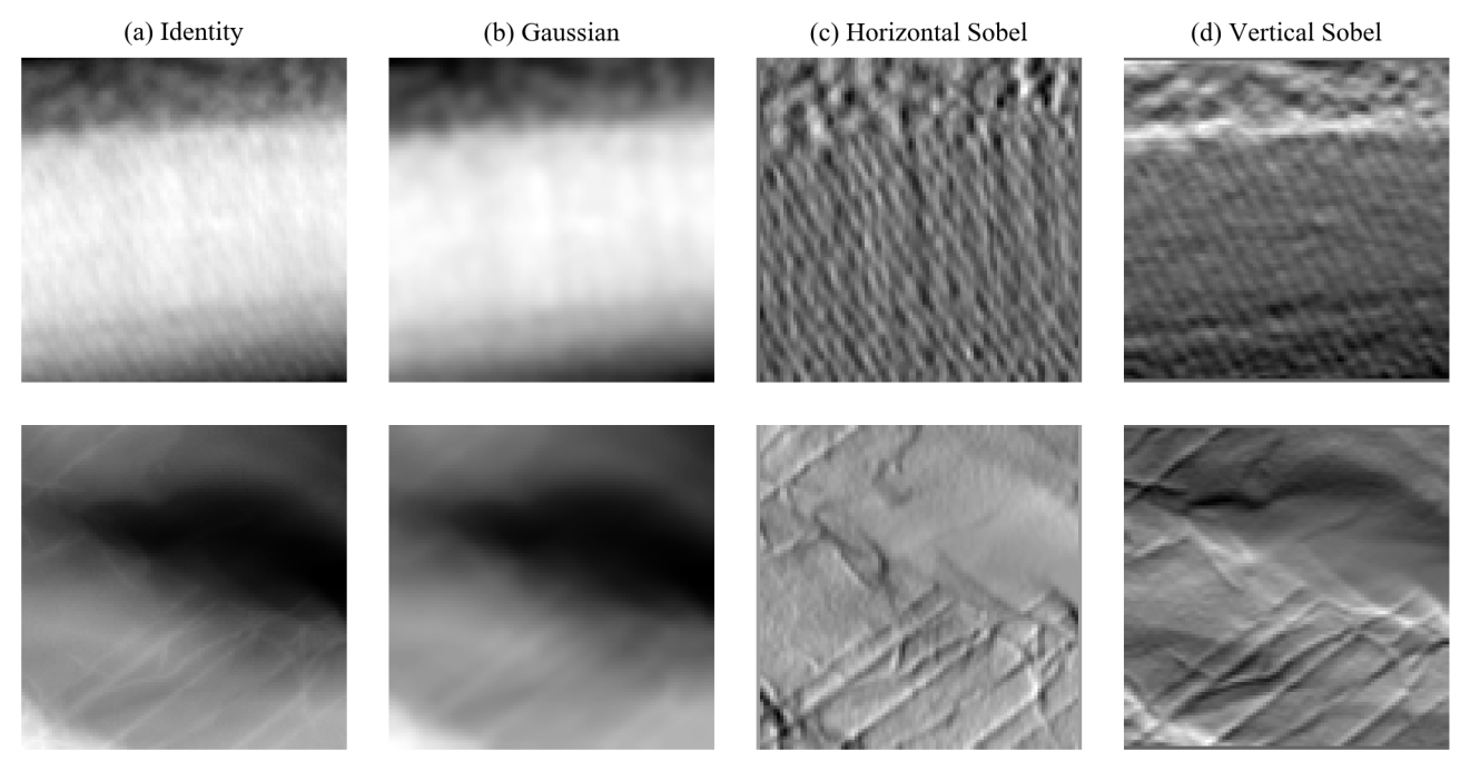
Kernels designed by humans[1057] are often convolved in image processing pipelines. For example, convolutions of electron micrographs with Gaussian and Sobel kernels are shown in figure 9. Gaussian kernels compute local averages, blurring images and suppressing high-frequency noise. For example, a 55 symmetric Gaussian kernel with a 2.5 px standard deviation is
| (38) |
Alternatives to Gaussian kernels for image smoothing[1058] include mean, median and bilateral filters. Sobel kernels compute horizontal and vertical spatial gradients that can be used for edge detection[1059]. For example, 33 Sobel kernels are
|
Alternatives to Sobel kernels offer similar utility, and include extended Sobel[1060], Scharr[1061, 1062], Kayyali[1063], Roberts cross[1064] and Prewitt[1065] kernels. Two-dimensional Gaussian and Sobel kernels are examples of linearly separable, or “flattenable”, kernels, which can be split into two one-dimensional kernels, as shown in equations 38-39b. Kernel separation can decrease computation in convolutional layers by convolving separated kernels in series, and CNNs that only use separable convolutions are effective[1066, 1067, 1068]. However, serial convolutions decrease parallelization and separable kernels have fewer degrees of freedom, decreasing representational capacity. Thus, separated kernels are usually at least 55, and separated 33 kernels are unusual. Even-sized kernels, such as 22 and 44, are rare as symmetric padding is needed to avoid information erosion caused by spatial shifts of feature maps[1069].
A traditional 2D convolutional layer maps inputs, , with height , width, , and depth, , to
| (40) |
where output channels are indexed by , is the sum of a bias, , and convolutions of each input channel with kernels with weights, . For clarity, a traditional convolutional layer is visualized in figure 8a. Convolutional layers for 1D, 3D and higher-dimensional kernels[1070] have a similar form to 2D kernels, where kernels are convolved across each dimension. Most inputs to convolutional layers are padded[1071, 1072] to avoid reducing spatial resolutions by kernel sizes, which could remove all resolution in deep networks. Padding is computationally inexpensive and eases implementations of ANNs that would otherwise combine layers with different sizes, such as FractalNet[1073], Inception[1074, 1075, 1076], NASNet[1077], recursive CNNs[1078, 1079], and ResNet[1080]. Pre-padding inputs results in higher performance than post-padding outputs[1081]. Following AlexNet[71], most convolutional layers are padded with zeros for simplicity. Reflection and replication padding achieve similar results to zero padding[1072]. However, padding based on partial convolutions[1082] consistently outperforms other methods[1072].
Convolutional layers are similar to fully connected layers used in multilayer perceptrons[1083, 1084] (MLPs). For comparison with equation 40, a fully connected, or “dense”, layer in a MLP computes
| (41) |
where every input element is connected to every output element. Convolutional layers reduce computation by making local connections within receptive fields of convolutional kernels, and by convolving kernels rather than using different weights at each input position. Intermediately, fully connected layers can be regularized to learn local connections[1085]. Fully connected layers are sometimes used at the middle of encoder-decoders[1086]. However, such fully connected layers can often be replaced by multiscale atrous, or “holey”, convolutions[955] in an atrous spatial pyramid pooling[306, 305] (ASPP) module to decrease computation without a significant decrease in performance. Alternatively, weights in fully connected layers can be decomposed into multiple smaller tensors to decrease computation without significantly decreasing performance[1087, 1088].
Convolutional layers can perform a variety of convolutional arithmetic[955]. For example, strided convolutions[1089] usually skip computation of outputs that are not at multiples of an integer spatial stride. Most strided convolutional layers are applied throughout CNNs to sequentially decrease spatial extent, and thereby decrease computational requirements. In addition, strided convolutions are often applied at the start of CNNs[1074, 539, 1075, 1076] where most input features can be resolved at a lower resolution than the input. For simplicity and computational efficiency, stride is typically constant within a convolutional layer; however, increasing stride away from the centre of layers can improve performance[1090]. To increase spatial resolution, convolutional layers often use reciprocals of integer strides[1091]. Alternatively, spatial resolution can be increased by combining interpolative upsampling with an unstrided convolutional layer[1092, 1093], which can help to minimize output artefacts.
Convolutional layers couple the computation of spatial and cross-channel convolutions. However, partial decoupling of spatial and cross-channel convolutions by distributing inputs across multiple convolutional layers and combining outputs can improve performance. Partial decoupling of convolutions is prevalent in many seminal DNN architectures, including FractalNet[1073], Inception[1074, 1075, 1076], NASNet[1077]. Taking decoupling to an extreme, depthwise separable convolutions[539, 1094, 1095] shown in figure 8b compute depthwise convolutions,
| (42) |
then compute pointwise 11 convolutions for intermediate channels,
| (43) |
where output channels are indexed by . Depthwise convolution kernels have weights, , and the depthwise layer is often followed by extra batch normalization before pointwise convolution to improve performance and accelerate convergence[1094]. Increasing numbers of channels with pointwise convolutions can increase accuracy[1094], at the cost of increased computation. Pointwise convolutions are a special case of traditional convolutional layers in equation 40 and have convolution kernel weights, , and add biases, . Naively, depthwise separable convolutions require fewer weight multiplications than traditional convolutions[1096, 1097]. However, extra batch normalization and serialization of one convolutional layer into depthwise and pointwise convolutional layers mean that depthwise separable convolutions and traditional convolutions have similar computing times[539, 1097].
Most DNNs developed for computer vision use fixed-size inputs. Although fixed input sizes are often regarded as an artificial constraint, it is similar to animalian vision where there is an effectively constant number of retinal rods and cones[1098, 1099, 1100]. Typically, the most practical approach to handle arbitrary image shapes is to train a DNN with crops so that it can be tiled across images. In some cases, a combination of cropping, padding and interpolative resizing can also be used. To fully utilize unmodified variable size inputs, a simple is approach to train convolutional layers on variable size inputs. A pooling layer, such as global average pooling, can then be applied to fix output size before fully connected or other layers that might require fixed-size inputs. More involved approaches include spatial pyramid pooling[1101] or scale RNNs[1102]. However, typical electron micrographs are much larger than 299299, which often makes it unfeasible for electron microscopists with a few GPUs to train high-performance DNNs on full-size images. For comparison, Xception was trained on 299299 images with 60 K80 GPUs for over one month.
The Fourier transform[1103], , at an -dimensional Fourier space vector, , is related to a function, , of an -dimensional signal domain vector, , by
| (44) | ||||
| (45) |
where , and is the imaginary number. Two parameters, and , can parameterize popular conventions that relate the Fourier and inverse Fourier transforms. Mathematica documentation nominates conventions[1104] for general applications , pure mathematics , classical physics , modern physics , systems engineering , and signal processing . We observe that most electron microscopists follow the modern physics convention of and ; however, the choice of convention is arbitrary and does not matter if it is consistent within a project. For discrete functions, Fourier integrals are replaced with summations that are limited to the support of a function.
Discrete Fourier transforms of uniformly spaced inputs are often computed with a fast Fourier transform (FFT) algorithm, which can be parallelized for CPUs[1105] or GPUs[65, 1106, 1107, 1108]. Typically, the speedup of FFTs on GPUs over CPUs is higher for larger signals[1109, 1110]. Most popular FFTs are based on the Cooley-Turkey algorithm[1111, 1112], which recursively divides FFTs into smaller FFTs. We observe that some electron microscopists consider FFTs to be limited to radix-2 signals that can be recursively halved; however, FFTs can use any combination of factors for the sizes of recursively smaller FFTs. For example, clFFT[1113] FFT algorithms support signal sizes that are any sum of powers of 2, 3, 5, 7, 11 and 13.
Convolution theorems can decrease computation by enabling convolution in the Fourier domain[1114]. To ease notation, we denote the Fourier transform of a signal, I, by , and the inverse Fourier transform by . Thus, the convolution theorems for two signals, and , are[1115]
| (46) | ||||
| (47) |
where the signals can be feature channels and convolutional kernels. Fourier domain convolutions, , are increasingly efficient, relative to signal domain convolutions, as kernel and image sizes increase[1114]. Indeed, Fourier domain convolutions are exploited to enable faster training with large kernels in Fourier CNNs[1116, 1114]. However, Fourier CNNs are rare as most researchers use small 33 kernels, following University of Oxford Visual Geometry Group (VGG) CNNs[1117].

4.4 Skip Connections
Residual connections[1080] add a signal after skipping ANN layers, similar to cortical skip connections[1118, 1119]. Residuals improve DNN performance by preserving gradient norms during backpropagation[1120, 537] and avoiding bad local minima[1121] by smoothing DNN loss landscapes[1122]. In practice, residuals enable DNNs to behave like an ensemble of shallow networks[1123] that learn to iteratively estimate outputs[1124]. Mathematically, a residual layer learns parameters, , of a perturbative function, , that maps a signal, , at depth to depth ,
| (48) |
Residuals were developed for CNNs[1080], and examples of residual connections that skip one, two and three convolutional layers are shown in figure 10. Nonetheless, residuals are also used in MLPs[1125] and RNNs[1126, 1127, 1128]. Representational capacity of perturbative functions increases as the number of skipped layers increases. As result, most residuals skip two or three layers. Skipping one layer rarely improves performance due to its low representational capacity[1080].
There are a range of residual connection variants that can improve performance. For example, highway networks[1129, 1130] apply a gating function to skip connections, and dense networks[1131, 1132, 1133] use a high number of residual connections from multiple layers. Another example is applying a 11 convolutional layer to before addition[1080, 539] where spatially resizes or changes numbers of feature channels. However, resizing with norm-preserving convolutional layers[1120] before residual blocks can often improve performance. Finally, long additive[1134] residuals that connect DNN inputs to outputs are often applied to DNNs that learn perturbative functions.
A limitation of preserving signal information with residuals[1135, 1136] is that residuals make DNNs learn perturbative functions, which can limit accuracy of DNNs that learn non-perturbative functions if they do not have many layers. Feature channel concatenation is an alternative approach that is not perturbative, and that supports combination of layers with different numbers of feature channels. In encoder-decoders, a typical example is concatenating features computed near the start with layers near the end to help resolve output features[316, 305, 306, 308]. Concatenation can also combine embeddings of different[1137, 1138] or variants of[366] input features from multiple DNNs. Finally, peephole connections in RNNs can improve performance by using concatenation to combine cell state information with other cell inputs[1139, 1140].
5 Architecture
There is a high variety of ANN architectures[4, 5, 6, 7] that are trained to minimize losses for a range of applications. Many of the most popular ANNs are also the simplest, and information about them is readily available. For example, encoder-decoder[502, 503, 305, 306, 307, 308, 504] or classifier[272] ANNs usually consist of single feedforward sequences of layers that map inputs to outputs. This section introduces more advanced ANNs used in electron microscopy, including actor-critics, GANs, RNNs, and variational autoencoders (VAEs). These ANNs share weights between layers or consist of multiple subnetworks. Other notable architectures include recursive CNNs[1078, 1079], Network-in-Networks[1141] (NiNs), and transformers[1142, 1143]. Although they will not be detailed in this review, their references may be good starting points for research.

5.1 Actor-Critic
Most ANNs are trained by gradient descent using backpropagated gradients of a differentiable loss function cf. section 6.1. However, some losses are not differentiable. Examples include losses of actors directing their vision[1144, 1145], and playing competitive[24] or score-based[1146, 1147] computer games. To overcome this limitation, a critic[1148] can be trained to predict differentiable losses from action and state information, as shown in figure 11. If the critic does not depend on states, it is a surrogate loss function[1149, 1150]. Surrogates are often fully trained before actor optimization, whereas critics that depend on actor-state pairs are often trained alongside actors to minimize the impact of catastrophic forgetting[1151] by adapting to changing actor policies and experiences. Alternatively, critics can be trained with features output by intermediate layers of actors to generate synthetic gradients for backpropagation[1152].

5.2 Generative Adversarial Network
Generative adversarial networks[197, 198, 199, 200] (GANs) consist of generator and discriminator subnetworks that play an adversarial game, as shown in figure 12. Generators learn to generate outputs that look realistic to discriminators, whereas discriminators learn to predict whether examples are real or generated. Most GANs are developed to generate visual media with realistic characteristics. For example, partial STEM images infilled with a GAN are less blurry than images infilled with a non-adversarial generator trained to minimize MSEs[201] cf. figure 2. Alternatively, computationally inexpensive loss functions designed by humans, such as structural similarity index measures[1153] (SSIMs) and Sobel losses[231], can improve generated output realism. However, it follows from the universal approximator theorems[37, 38, 39, 40, 41, 42, 43, 44, 45] that training with ANN discriminators can often yield more realistic outputs.
There are many popular GAN loss functions and regularization mechanisms[1154, 1155, 1156, 1157, 1158]. Traditionally, GANs were trained to minimize logarithmic discriminator, , and generator, , losses[1159],
| (49) | ||||
| (50) |
where z are generator inputs, are generated outputs, and x are example outputs. Discriminators predict labels, and , where target labels are 0 and 1 for generated and real examples, respectively. Limitedly, logarithmic losses are numerically unstable for or , as the denominator, , in vanishes. In addition, discriminators must be limited to and , so that logarithms are not complex. To avoid these issues, we recommend training discriminators with squared difference losses[1160, 1161],
| (51) | ||||
| (52) |
However, there are a variety of other alternatives to logarithmic loss functions that are also effective[1154, 1155].
A variety of methods have been developed to improve GAN training[1162, 995]. The most common issues are catastrophic forgetting[1151] of previous learning, and mode collapse[1163] where generators only output examples for a subset of a target domain. Mode collapse often follows discriminators becoming Lipschitz discontinuous. Wasserstein GANs[1164] avoid mode collapse by clipping trainable variables, albeit often at the cost of 5-10 discriminator training iterations per generator training iteration. Alternatively, Lipschitz continuity can be imposed by adding a gradient penalty[1165] to GAN losses, such as differences of L2 norms of discriminator gradients from unity,
| (53) | ||||
| (54) | ||||
| (55) | ||||
| (56) |
where is a uniform random variate, weights the gradient penalty, and is an attempt to generate . However, using a gradient penalty introduces additional gradient backpropagation that increases discriminator training time. There are also a variety of computationally inexpensive tricks that can improve training, such as adding noise to labels[995, 1075, 1166] or balancing discriminator and generator learning rates[349]. These tricks can help to avoid discontinuities in discriminator output distributions that can lead to mode collapse; however, we observe that these tricks do not reliably stabilize GAN training.
Instead, we observe that spectral normalization[1017] reliably stabilizes GAN discriminator training in our electron microscopy research[201, 349, 202]. Spectral normalization controls Lipschitz constants of discriminators by fixing the spectral norms of their weights, as introduced in section 4.2. Advantages of spectral normalization include implementations based on the power iteration method[1023, 1024] being computationally inexpensive, not adding a regularizing loss function that could detrimentally compete[1167, 1168] with discrimination losses, and being effective with one discriminator training iterations per generator training iteration[1017, 1169]. Spectral normalization is popular in GANs for high-resolution image synthesis, where it is also applied in generators to stabilize training[1170].
There are a variety of GAN architectures[1171]. For high-resolution image synthesis, computation can be decreased by training multiple discriminators to examine image patches at different scales[1172, 201]. For domain translation characterized by textural differences, a cyclic GAN[1004, 1173] consisting of two GANs can map from one domain to the other and vice versa. Alternatively, two GANs can share intermediate layers to translate inputs via a shared embedding domain[1174]. Cyclic GANs can also be combined with a siamese network[279, 280, 281] for domain translation beyond textural differences[1175]. Finally, discriminators can introduce auxiliary losses to train DNNs to generalize to examples from unseen domains[1176, 1177, 1178].

5.3 Recurrent Neural Network
Recurrent neural networks[531, 532, 533, 534, 535, 536] reuse an ANN cell to process each step of a sequence. Most RNNs learn to model long-term dependencies by gradient backpropagation through time[1179] (BPTT). The ability of RNNs to utilize past experiences enables them to model partially observed and variable length Markov decision processes[1180, 1181] (MDPs). Applications of RNNs include directing vision[1144, 1145], image captioning[1182, 1183], language translation[1184], medicine[77], natural language processing[1185, 1186], playing computer games[24], text classification[1055], and traffic forecasting[1187]. Many RNNs are combined with CNNs to embed visual media[1145] or words[1188, 1189], or to process RNN outputs[1190, 1191]. RNNs can also be combined with MLPs[1144], or text embeddings[1192] such as BERT[1193, 1192], continuous bag-of-words[1194, 1195, 1196] (CBOW), doc2vec[1197, 1198], GloVe[1199], and word2vec[1200, 1194].
The most popular RNNs consist of long short-term memory[1201, 1202, 1203, 1204] (LSTM) cells or gated recurrent units[1202, 1205, 1206, 1207] (GRUs). LSTMs and GRUs are popular as they solve the vanishing gradient problem[1208, 1209, 537] and have consistently high performance[1210, 1211, 1212, 1213, 1214, 1215]. Their architectures are shown in figure 13. At step , an LSTM outputs a hidden state, , and cell state, , given by
| (57) | ||||
| (58) | ||||
| (59) | ||||
| (60) | ||||
| (61) | ||||
| (62) |
where is the previous cell state, is the previous hidden state, is the step input, and is a logistic sigmoid function of equation 10a, is the concatenation of x and y channels, and , , and are pairs of weights and biases. A GRU performs fewer computations than an LSTM and does not have separate cell and hidden states,
| (63) | ||||
| (64) | ||||
| (65) | ||||
| (66) |
where , , and are pairs of weights and biases. Minimal gated units (MGUs) can further reduce computation[1216]. A large-scale analysis of RNN architectures for language translation found that LSTMs consistently outperform GRUs[1210]. GRUs struggle with simple languages that are learnable by LSTMs as the combined hidden and cell states of GRUs make it more difficult for GRUs to perform unbounded counting[1214]. However, further investigations found that GRUs can outperform LSTMs on tasks other than language translation[1211], and that GRUs can outperform LSTMs on some datasets[1217, 1212, 1213]. Overall, LSTM performance is usually comparable to that of GRUs.
There are a variety of alternatives to LSTM and GRUs. Examples include continuous time RNNs[1218, 1219, 1220, 1221, 1222] (CTRNNs), Elman[1223] and Jordan[1224] networks, independently RNNs[1225] (IndRNNs), Hopfield networks[1226], recurrent MLPs[1227] (RMLPs). However, none of the variants offer consistent performance benefits over LSTMs for general sequence modelling. Similarly, augmenting LSTMs with additional connections, such as peepholes[1139, 1140] and projection layers[1228], does not consistently improve performance. For electron microscopy, we recommend defaulting to LSTMs as we observe that their performance is more consistently high than performance of other RNNs. However, LSTM and GRU performance is often comparable, so GRUs are also a good choice to reduce computation.
There are a variety of architectures based on RNNs. Popular examples include deep RNNs[1229] that stack RNN cells to increase representational ability, bidirectional RNNs[1230, 1231, 1232, 1233] that process sequences both forwards and in reverse to improve input utilization, and using separate encoder and decoder subnetworks[1205, 1234] to embed inputs and generate outputs. Hierarchical RNNs[1235, 1236, 1237, 1238, 1239] are more complex models that stack RNNs to efficiently exploit hierarchical sequence information, and include multiple timescale RNNs[1240, 1241] (MTRNNs) that operate at multiple sequence length scales. Finally, RNNs can be augmented with additional functionality to enable new capabilities. For example, attention[1242, 1243, 1244, 1182] mechanisms can enable more efficient input utilization. Further, creating a neural Turing machine (NTM) by augmenting a RNN with dynamic external memory[1245, 1246] can make it easier for an agent to solve dynamic graphs.

5.4 Autoencoders
Autoencoders[1247, 1248, 1249] (AEs) learn to efficiently encode inputs, I, without supervision. An AE consists of a encoder, , and decoder, , as shown in figure 14a. Most encoders and decoders are jointly trained[1250] to restore inputs from encodings, , to minimize a MSE loss,
| (67) |
by gradient descent. In practice, DNN encoders and decoders yield better compression[1248] than linear techniques, such as principal component analysis[1251] (PCA), or shallow ANNs. Indeed, deep AEs can outperform JPEG image compression[1252]. Denoising autoencoders[1253, 1254, 1255, 1256, 1257] (DAEs) are a popular AE variant that can learn to remove artefacts by artificially corrupting inputs inside encoders. Alternatively, contractive autoencoders[1258, 1259] (CAEs) can decrease sensitivity to input values by adding a loss to minimize gradients w.r.t. inputs. Most DNNs that improve electron micrograph signal-to-noise are DAEs.
In general, semantics of AE outputs are pathological functions of encodings. To generate outputs with well-behaved semantics, traditional VAEs[969, 1260, 1261] learn to encode means, , and standard deviations, , of Gaussian multivariates. Meanwhile, decoders learn to reconstruct inputs from sampled multivariates, , where is a standard normal multivariate. Traditional VAE architecture is shown in figure 14b. Usually, VAE encodings are regularized by adding Kullback-Leibler (KL) divergence of encodings from standard multinormals to an AE loss function,
| (68) |
where weights the contribution of the KL divergence loss for a batch size of , and a latent space with degrees of freedom. However, variants of Gaussian regularization can improve clustering[231], and sparse autoencoders[1262, 1263, 1264, 1265] (SAEs) that regularize encoding sparsity can encode more meaningful features. To generate realistic outputs, a VAE can be combined with a GAN to create a VAE-GAN[1266, 1267, 1268]. Adding a loss to minimize differences between gradients of generated and target outputs is computationally inexpensive alternative that can generate realistic outputs for some applications[231].
A popular application of VAEs is data clustering. For example, VAEs can encode hash tables[1269, 1270, 1271, 1272, 1273] for search engines, and we use VAEs as the basis of our electron micrograph search engines[231]. Encoding clusters visualized by tSNE can be labelled to classify data[231], and encoding deviations from clusters can be used for anomaly detection[1274, 1275, 1276, 1277, 1278]. In addition, learning encodings with well-behaved semantics enables encodings to be used for semantic manipulation[1279, 1278]. Finally, VAEs can be used as generative models to create synthetic populations[1280, 1281], develop new chemicals[1282, 1283, 1284, 1285], and synthesize underrepresented data to reduce imbalanced learning[1286].
6 Optimization
Training, testing, deployment and maintenance of machine learning systems is often time-consuming and expensive[1287, 1288, 1289, 1290]. The first step is usually preparing training data and setting up data pipelines for ANN training and evaluation. Typically, ANN parameters are randomly initialized for optimization by gradient descent, possibly as part of an automatic machine learning algorithm. Reinforcement learning is a special optimization case where the loss is a discounted future reward. During training, ANN components are often regularized to stabilize training, accelerate convergence, or improve performance. Finally, trained models can be streamlined for efficient deployment. This section introduces each step. We find that electron microscopists can be apprehensive about robustness and interpretability of ANNs, so we also provide subsections on model evaluation and interpretation.

6.1 Gradient Descent
Most ANNs are iteratively trained by gradient descent[1303, 1304, 1305, 465, 1306, 1307], as described by algorithm 1 and shown in figure 15. To minimize computation, results at intermediate stages of forward propagation, where inputs are mapped to outputs, are often stored in memory. Storing the forwards pass in memory enables backpropagation memoization by sequentially computing gradients w.r.t. trainable parameters. To reduce memory costs for large ANNs, a subset of intermediate forwards pass results can be saved as starting points to recompute other stages during backpropagation[1308, 1309]. Alternatively, forward pass computations can be split across multiple devices[1310]. Optimization by gradient descent plausibly models learning in some biological systems[1311]. However, gradient descent is not generally an accurate model of biological learning[1312, 1313, 1314].
There are many popular gradient descent optimizers for deep learning[1303, 1304, 1305]. Update rules for eight popular optimizers are summarized in figure 1. Other optimizers include AdaBound[1315], AMSBound[1315], AMSGrad[1316], Lookahead[1317], NADAM[1318], Nostalgic Adam[1319], Power Gradient Descent[1320], Rectified ADAM[1321] (RADAM), and trainable optimizers[1322, 1323, 1324, 1325, 1326]. Gradient descent is effective in the high-dimensional optimization spaces of overparameterized ANNs[1327] as the probability of getting trapped in a sub-optimal local minima decreases as the number of dimensions increases. The simplest optimizer is “vanilla” stochastic gradient descent (SGD), where a trainable parameter perturbation, , is the product of a learning rate, , and derivative of a loss, , w.r.t. the trainable parameter, . However, vanilla SGD convergence is often limited by unstable parameter oscillations as it a low-order local optimization method[1328]. Further, vanilla SGD has no mechanism to adapt to varying gradient sizes, which vary effective learning rates as .
To accelerate convergence, many optimizers introduce a momentum term that weights an average of gradients with past gradients[1329, 1296, 1330]. Momentum-based optimizers in figure 1 are momentum, Nesterov momentum[1296, 1297], quasi-hyperbolic momentum[1299], AggMo[1300], ADAM[1302], and AdaMax[1302]. To standardize effective learning rates for every layer, adaptive optimizers normalize updates based on an average of past gradient sizes. Adaptive optimizers in figure 1 are RMSProp[1301], ADAM[1302], and AdaMax[1302], which usually result in faster convergence and higher accuracy than other optimizers[1331, 1332]. However, adaptive optimizers can be outperformed by vanilla SGD due to overfitting[1333], so some researchers adapt adaptive learning rates to their variance[1321] or transition from adaptive optimization to vanilla SGD as training progresses[1315]. For electron microscopy we recommend adaptive optimization with Nadam[1318], which combines ADAM with Nesterov momentum, as it is well-established and a comparative analysis of select gradient descent optimizers found that it often achieves higher performance than other popular optimizers[1334]. Limitingly, most adaptive optimizers slowly adapt to changing gradient sizes e.g. a default value for ADAM is 0.999[1302]. To prevent learning being destabilized by spikes in gradient sizes, adaptive optimizers can be combined with adaptive learning rate[261, 1315] or gradient[1335, 1208, 1336] clipping.
For non-adaptive optimizers, effective learning rates are likely to vary due to varying magnitudes of gradients w.r.t. trainable parameters. Similarly, learning by biological neurons varies as stimuli usually activate a subset of neurons[1337]. However, all neuron outputs are usually computed for ANNs. Thus, not effectively using all weights to inform decisions is computational inefficient. Further, inefficient weight updates can limit representation capacity, slow convergence, and decrease training stability. A typical example is effective learning rates varying between layers. Following the chain rule, gradients backpropagated to the th layer of a DNN from its start are
| (90) |
for a DNN with layers. Vanishing gradients[1209, 537, 1208] occur when many layers have . For example, DNNs with logistic sigmoid activations often exhibit vanishing gradients as their maximum gradient is cf. equation 10b. Similarly, exploding gradients[1209, 537, 1208] occur when many layers have . Adaptive optimizers alleviate vanishing and exploding gradients by dividing gradients by their expected sizes. Nevertheless, it is essential to combine adaptive optimizers with appropriate initialization and architecture to avoid numerical instability.
Optimizers have a myriad of hyperparameters to be initialized and varied throughout training to optimize performance[1338] cf. figure 1. For example, stepwise exponentially decayed learning rates are often theoretically optimal[1339]. There are also various heuristics that are often effective, such as using a DEMON decay schedule for an ADAM first moment of the momentum decay rate[1340],
| (91) |
where is the initial value of , is the iteration number, and is the final iteration number. Developers often optimize ANN hyperparameters by experimenting with a range of heuristic values. Hyperparameter optimization algorithms[1341, 1342, 1343, 1344, 1345, 1346] can automate optimizer hyperparameter selection. However, automatic hyperparameter optimizers may not yield sufficient performance improvements relative to well-established heuristics to justify their use, especially in initial stages of development.
Alternatives to gradient descent[1347] are rarely used for parameter optimization as they are not known to consistently improve upon gradient descent. For example, simulated annealing[1348, 1349] has been applied to CNN training[1350, 1351], and can be augmented with momentum to accelerate convergence in deep learning[1352]. Simulated annealing can also augment gradient descent to improve performance[1353]. Other approaches include evolutionary[1354, 1355] and genetic[1356, 1357] algorithms, which can be a competitive alternative to deep reinforcement learning where convergence is slow[1358]. Indeed, recent genetic algorithms have outperformed a popular deep reinforcement learning algorithm[1359]. Another direction is to augment genetic algorithms with ANNs to accelerate convergence[1360, 1361, 1362, 1363]. Other alternatives to backpropagation include direct search[1364], the Moore-Penrose Pseudo Inverse[1365]; particle swarm optimization[1366, 1367, 1368, 1369] (PSO); and echo-state networks[1370, 1371, 1372] (ESNs) and extreme learning machines[1373, 1374, 1375, 1376, 1377, 1378, 1379] (ELMs), where some randomly initialized weights are never updated.
6.2 Reinforcement Learning
Reinforcement learning[1380, 1381, 1382, 1383, 1384, 1385, 1386] (RL) is where a machine learning system, or “actor”, is trained to perform a sequence of actions. Applications include autonomous driving[1387, 1388, 1389], communications network control[1390, 1391], energy and environmental management[1392, 1393], playing games[24, 25, 26, 27, 1394, 1146, 28, 29], and robotic manipulation[1395, 1396]. To optimize a MDP[1180, 1181], a discounted future reward, , at step in a MDP with steps is usually calculated from step rewards, , with Bellman’s equation,
| (92) |
where discounts future step rewards. To be clear, multiplying by yields a loss that can be minimized using the methods in section 6.1.
In practice, many MDPs are partially observed or have non-differentiable losses that may make it difficult to learn a good policy from individual observations. However, RNNs can often learn a model of their environments from sequences of observations[1147]. Alternatively, FNNs can be trained with groups of observations that contain more information than individual observations[1394, 1146]. If losses are not differentiable, a critic can learn to predict differentiable losses for actor training cf. section 5.1. Alternatively, actions can be sampled from a differentiable probability distribution[1397, 1144] as training losses given by products of losses and sampling probabilities are differentiable. There are also a variety of alternatives to gradient descent introduced at the end of section 6.1 that do not require differentiable loss functions.
There are a variety of exploration strategies for RL[1398, 1399]. Adding Ornstein-Uhlenbeck[1400] (OU) noise to actions is effective for continuous control tasks optimized by deep deterministic policy gradients[1146] (DDPG) or recurrent deterministic policy gradients[1147] (RDPG) RL algorithms. Adding Gaussian noise achieves similar performance for optimization by TD3[1401] or D4PG[1402] RL algorithms. However, a comparison of OU and Gaussian noise across a variety of tasks[1403] found that OU noise usually achieves similar performance to or outperforms Gaussian noise. Similarly, exploration can be induced by adding noise to ANN parameters[1404, 1405]. Other approaches to exploration include rewarding actors for increasing action entropy[1406, 1407, 1405] and intrinsic motivation[1408, 1409, 1410], where ANNs are incentified to explore actions that they are unsure about.
RL algorithms are often partitioned into online learning[1411, 1412], where training data is used as it is acquired; and offline learning[1413, 1414], where a static training dataset has already been acquired. However, many algorithms operate in an intermediate regime, where data collected with an online policy is stored in an experience replay[1415, 1416, 1417] buffer for offline learning. Training data is often sampled at random from a replay. However, prioritizing the replay of data with high losses[993] or data that results in high policy improvements[992] often improves actor performance. A default replay buffer size of around examples is often used; however, training is sensitive to replay buffer size[1418]. If the replay is too small, changes in actor policy may destabilize training; whereas if the replay is too large, convergence may be slowed by delays before the actor learns from policy changes.
6.3 Automatic Machine Learning
There are a variety of automatic machine learning[1419, 1420, 1421, 1422, 1423] (AutoML) algorithms that can create and optimize ANN architectures and learning policies for a dataset of input and target output pairs. Most AutoML algorithms are based on RL or evolutionary algorithms. Examples of AutoML algorithms include AdaNet[1424, 1425], Auto-DeepLab[1426], AutoGAN[1427], Auto-Keras[1428], auto-sklearn[1429], DARTS+[1430], EvoCNN[271], H2O[1431], Ludwig[1432], MENNDL[1433, 1434], NASBOT[1435], XNAS[1436], and others[1437, 1438, 1439, 1440, 1441]. AutoML is becoming increasingly popular as it can achieve higher performance than human developers[1442, 1077] and enables human developer time to be traded for potentially cheaper computer time. Nevertheless, AutoML is currently limited to established ANN architectures and learning policies. Consequently, we recommend that researchers either focus on novel ANN architectures and learning policies or developing ANNs for novel applications.
6.4 Initialization
How ANN trainable parameters are initialized[537, 1443] is related to model capacity[1444]. Further, initializing parameters with values that are too small or large can cause slow learning or divergence[537]. Careful initialization can also prevent training by gradient descent being destabilized by vanishing or exploding gradients[1209, 537, 1208], or high variance of length scales across layers[537]. Finally, careful initialization can enable momentum to accelerate convergence and improve performance[1296]. Most trainable parameters are multiplicative weights or additive biases. Initializing parameters with constant values can result in every parameter in a layer receiving the same updates by gradient descent, reducing model capacity. Thus, weights are often randomly initialized. Followingly, biases are often initialized with constant values due to symmetry breaking by the weights.
Consider the projection of inputs, , to outputs, , by an weight matrix, w. The expected variance of an output element is[1443]
| (93) |
where and denote the expected mean and variance of elements of x, respectively. For similar length scales across layers, should be constant. Initially, similar variances can be achieved by normalizing ANN inputs to have zero mean, so that , and initializing weights so that and . However, parameters can shift during training, destabilizing learning. To compensate for parameter shift, popular normalization layers like batch normalization often impose and , relaxing need for or . Nevertheless, training will still be sensitive to the length scale of trainable parameters.
There are a variety of popular weight initializers that adapt weights to ANN architecture. One of the oldest methods is LeCun initialization[951, 941], where weights are initialized with variance,
| (94) |
which is argued to produce outputs with similar length scales in the previous paragraph. However, a similar argument can be made for initializing with to produce similar gradients at each layer during the backwards pass[1443]. As a compromise, Xavier initialization[1445] computes an average,
| (95) |
However, adjusting weights for is not necessary for adaptive optimizers like ADAM, which divide gradients by their length scales, unless gradients will vanish or explode. Finally, He initialization[22] doubles the variance of weights to
| (96) |
and is often used in ReLU networks to compensate for activation functions halving variances of their outputs[22, 1446, 1443]. Most trainable parameters are initialized from either a zero-centred Gaussian or uniform distribution. For convenience, the limits of such a uniform distribution are . Uniform initialization can outperform Gaussian initialization in DNNs due to Gaussian outliers harming learning[1443]. However, issues can be avoided by truncating Gaussian initialization, often to two standard deviations, and rescaling to its original variance.
Some initializers are mainly used for RNNs. For example, orthogonal initialization[1447] often improves RNN training[1448] by reducing susceptibility to vanishing and exploding gradients. Similarly, identity initialization[1449, 1450] can help RNNs to learn long-term dependencies. In most ANNs, biases are initialized with zeros. However, the forget gates of LSTMs are often initialized with ones to decrease forgetting at the start of training[1211]. Finally, the start states of most RNNs are initialized with zeros or other constants. However, random multivariate or trainable variable start states can improve performance[1451].
There are a variety of alternatives to initialization from random multivariates. Weight normalized[1014] ANNs are a popular example of data-dependent initialization, where randomly initialized weight magnitudes and biases are chosen to counteract variances and means of an initial batch of data. Similarly, layer-sequential unit-variance (LSUV) initialization[1452] consists of orthogonal initialization followed by adjusting the magnitudes of weights to counteract variances of an initial batch of data. Other approaches standardize the norms of backpropagated gradients. For example, random walk initialization[1453] (RWI) finds scales for weights to prevent vanishing or exploding gradients in deep FNNs, albeit with varied success[1452]. Alternatively, MetaInit[1454] scales the magnitudes of randomly initialized weights to minimize changes in backpropagated gradients per iteration of gradient descent.
6.5 Regularization
There are a variety of regularization mechanisms[1455, 1456, 1457, 1458] that modify learning algorithms to improve ANN performance. One of the most popular is L regularization, which decays weights by adding a loss,
| (97) |
weighted by to each trainable variable, . L2 regularization[1459, 1460, 1461] is preferred[1462] for most DNN optimization as subtraction of its gradient, , is equivalent to computationally-efficient multiplicative weight decay. Nevertheless, L1 regularization is better at inducing model sparsity[1463] than L2 regularization, and L1 regularization achieves higher performance in some applications[1464]. Higher performance can also be achieved by adding both L1 and L2 regularization in elastic nets[1465]. L regularization is most effective at the start of training and becomes less important near convergence[1459]. Finally, L1 and L2 regularization are closely related to lasso[1466] and ridge[1467] regularization, respectively, whereby trainable parameters are adjusted to limit and losses.
Gradient clipping[1468, 1336, 1469, 1470] accelerates learning by limiting large gradients, and is most commonly applied to RNNs. A simple approach is to clip gradient magnitudes to a threshold hyperparameter. However, it is more common to scale gradients, , at layer if their norm is above a threshold, , so that[1208, 1469]
| (98) |
where is often chosen to minimize computation. Similarly, gradients can be clipped if they are above a global norm,
| (99) |
computed with gradients at layers. Scaling gradient norms is often preferable to clipping to a threshold as scaling is akin to adapting layer learning rates and does not affect the directions of gradients. Thresholds for gradient clipping are often set based on average norms of backpropagated gradients during preliminary training[1471]. However, thresholds can also be set automatically and adaptively[1335, 1336]. In addition, adaptive gradient clipping algorithms can skip training iterations if gradient norms are anomalously high[1472], which often indicates an imminent gradient explosion.
Dropout[1473, 1474, 1475, 1476, 1477] often reduces overfitting by only using a fraction, , of layer outputs during training, and multiplying all outputs by for inference. However, dropout often increases training time, can be sensitive to , and sometimes lowers performance[1478]. Improvements to dropout at the structural level, such as applying it to convolutional channels, paths, and layers, rather than random output elements, can improve performance[1479]. For example, DropBlock[1480] improves performance by dropping contiguous regions of feature maps to prevent dropout being trivially circumvented by using spatially correlated neighbouring outputs. Similarly, PatchUp[1481] swaps or mixes contiguous regions with regions for another sample. Dropout is often outperformed by Shakeout[1482, 1483], a modification of dropout that randomly enhances or reverses contributions of outputs to the next layer.
Noise often enhances ANN training by decreasing susceptibility to spurious local minima[1484]. Adding noise to trainable parameters can improve generalization[1485, 1486], or exploration for RL[1404]. Parameter noise is usually additive as it does not change an objective function being learned, whereas multiplicative noise can change the objective[1487]. In addition, noise can be added to inputs[1488, 1253], hidden layers[1489, 1158], generated outputs[1490] or target outputs[1491, 995]. However, adding noise to signals does not always improve performance[1217]. Finally, modifying usual gradient noise[1492] by adding noise to gradients can improve performance[1493]. Typically, additive noise is annealed throughout training, so that that final training is with a noiseless model that will be used for inference.
There are a variety of regularization mechanisms that exploit extra training data. A simple approach is to create extra training examples by data augmentation[1494, 1495, 1496]. Extra training data can also be curated, or simulated for training by domain adaption[1176, 1177, 1178]. Alternatively, semi-supervised learning[1497, 1498, 1499, 1500, 1501, 1502] can generate target outputs for a dataset of unpaired inputs to augment training with a dataset of paired inputs and target outputs. Finally, multitask learning[1503, 1504, 1505, 1506, 1507] can improve performance by introducing additional loss functions. For instance, by adding an auxiliary classifier to predict image labels from features generated by intermediate DNN layers[1508, 1509, 1510, 1511]. Losses are often manually balanced; however, their gradients can also be balanced automatically and adaptively[1167, 1168].
6.6 Data Pipeline
A data pipeline prepares data to be input to an ANN. Efficient pipelines often parallelize data preparation across multiple CPU cores[1512]. Small datasets can be stored in RAM to decrease data access times, whereas large dataset elements are often loaded from files. Loaded data can then be preprocessed and augmented[1513, 1495, 1494, 1514, 1515]. For electron micrographs, preprocessing often includes replacing non-finite elements, such as NaN and inf, with finite values; linearly transforming intensities to a common range, such as or zero mean and unit variance; and performing a random combination of flips and 90 rotations to augment data by a factor of eight[70, 349, 201, 231, 202]. Preprocessed examples can then be combined into batches. Typically, multiple batches that are ready to be input are prefetched and stored in RAM to avoid delays due to fluctuating CPU performance.
To efficiently utilize data, training datasets are often reiterated over for multiple training epochs. Usually, training datasets are reiterated over about times. Increasing epochs can maximize utilization of potentially expensive training data; however, increasing epochs can lower performance due to overfitting[1516, 1517] or be too computationally expensive[539]. Naively, batches of data can be randomly sampled with replacement during training by gradient descent. However, convergence can be accelerated by reinitializing a training dataset at the start of each training epoch and randomly sampling data without replacement[1518, 1519, 1520, 1521, 1522]. Most modern DLFs, such as TensorFlow, provide efficient and easy-to-use functions to control data sampling[1523].
6.7 Model Evaluation
There are a variety of methods for ANN performance evaluation[538]. However, most ANNs are evaluated by 1-fold validation, where a dataset is partitioned into training, validation, and test sets. After ANN optimization with a training set, ability to generalize is measured with a validation set. Multiple validations may be performed for training with early stopping[1516, 1517] or ANN learning policy and architecture selection, so final performance is often measured with a test set to avoid overfitting to the validation set. Most researchers favour using single training, validation, and test sets to simplify standardization of performance benchmarks[231]. However, multiple-fold validation[538] or multiple validation sets[1524] can improve performance characterization. Alternatively, models can be bootstrap aggregated[1525] (bagged) from multiple models trained on different subsets of training data. Bagging is usually applied to random forests[1526, 1527, 1528] or other lightweight models, and enables model uncertainly to be gauged from the variance of model outputs.
For small datasets, model performance is often sensitive to split of data between training and validation sets[1529]. Increasing training set size usually increases model accuracy, whereas increasing validation set size decreases performance uncertainty. Indeed, a scaling law can be used to estimate an optimal tradeoff[1530] between training and validation set sizes. However, most experimenters follow a Pareto[1531] splitting heuristic. For example, we often use a 75:15:10 training-validation-test split[231]. Heuristic splitting is justified for ANN training with large datasets insofar that sensitivity to splitting ratios decreases with increasing dataset size[2].
6.8 Deployment
If an ANN is deployed[1532, 1533, 1534] on multiple different devices, such as various electron microscopes, a separate model can be trained for each device[403], Alternatively, a single model can be trained and specialized for different devices to decrease training requirements[1535]. In addition, ANNs can remotely service requests from cloud containers[1536, 1537, 1538]. Integration of multiple ANNs can be complicated by different servers for different DLFs supporting different backends; however, unified interfaces are available. For example, GraphPipe[1539] provides simple, efficient reference model servers for Tensorflow, Caffe2, and ONNX; a minimalist machine learning transport specification based on FlatBuffers[1540]; and efficient client implementations in Go, Python, and Java. In 2020, most ANNs developed researchers were not deployed. However, we anticipate that deployment will become a more prominent consideration as the role of deep learning in electron microscopy matures.
Most ANNs are optimized for inference by minimizing parameters and operations from training time, like MobileNets[1094]. However, less essential operations can also be pruned after training[1541, 1542]. Another approach is quantization, where ANN bit depths are decreased, often to efficient integer instructions, to increase inference throughput[1543, 1544]. Quantization often decreases performance; however, the amount of quantization can be adapted to ANN components to optimize performance-throughput tradeoffs[1545]. Alternatively, training can be modified to minimize the impact of quantization on performance[1546, 1547, 1548]. Another approach is to specialize bit manipulation for deep learning. For example, signed brain floating point (bfloat16) often improves accuracy on TPUs by using an 8 bit mantissa and 7 bit exponent, rather than a usual 5 bit mantissa and 10 bit exponent[1549]. Finally, ANNs can be adaptively selected from a set of ANNs based on available resources to balance tradeoff of performance and inference time[1550], similar to image optimization for web applications[1551, 1552].
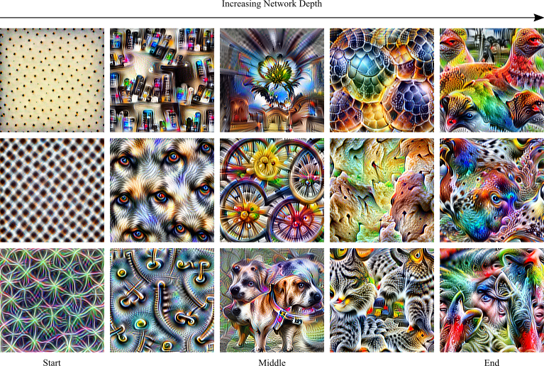
6.9 Interpretation
We find that some electron microscopists are apprehensive about working with ANNs due to a lack of interpretability, irrespective of rigorous ANN validation. We try to address uncertainty by providing loss visualizations in some of our electron microscopy papers[201, 70, 202]. However, there are a variety of popular approaches to explainable artificial intelligence[1554, 1555, 1556, 1557, 1558, 1559, 1560] (XAI). One of the most popular approaches to XAI is saliency[1561, 1562, 1563, 1564], where gradients of outputs w.r.t. inputs correlate with their importance. Saliency is often computed by gradient backpropagation[1565, 1566, 1567]. For example, with Grad-CAM[1568] or its variants[1569, 1570, 1571, 1572]. Alternatively, saliency can be predicted by ANNs[1054, 1573, 1574] or a variety of methods inspired by Grad-CAM[1575, 1576, 1577]. Applications of saliency include selecting useful features from a model[1578], and locating regions in inputs corresponding to ANN outputs[1579].
There are a variety of other approaches to XAI. For example, feature visualization via optimization[1553, 1580, 1581, 1582, 1583] can find inputs that maximally activate parts of an ANN, as shown in figure 16. Another approach is to cluster features, e.g. by tSNE[1584, 1585] with the Barnes-Hut algorithm[1586, 1587], and examine corresponding clustering of inputs or outputs[231]. Finally, developers can view raw features and gradients during forward and backward passes of gradient descent, respectively. For example, CNN explainer[1588, 1589] is an interactive visualization tool designed for non-experts to learn and experiment with CNNs. Similarly, GAN Lab[1590] is an interactive visualization tool for non-experts to learn and experiment with GANs.
7 Discussion
We introduced a variety of electron microscopy applications in section 1 that have been enabled or enhanced by deep learning. Nevertheless, the greatest benefit of deep learning in electron microscopy may be general-purpose tools that enable researchers to be more effective. Search engines based on deep learning are almost essential to navigate an ever-increasing number of scientific publications[700]. Further, machine learning can enhance communication by filtering spam and phishing attacks[1591, 1592, 1593], and by summarizing[1594, 1595, 1596] and classifying[1597, 1598, 1599, 1055] scientific documents. In addition, machine learning can be applied to education to automate and standardize scoring[1600, 1601, 1602, 1603], detect plagiarism[1604, 1605, 1606], and identify at-risk students[1607].
Creative applications of deep learning[1608, 1609] include making new art by style transfer[1001, 1002, 1003, 1004, 1005], composing music[1610, 1611, 1612], and storytelling[1613, 1614]. Similar DNNs can assist programmers[1615, 1616]. For example, by predictive source code completion[1617, 1618, 1619, 1620, 1621, 1622], and by generating source code to map inputs to target outputs[1623] or from labels describing desired source code[1624]. Text generating DNNs can also help write scientific papers. For example, by drafting scientific passages[1625] or drafting part of a paper from a list of references[1626]. Papers generated by early prototypes for automatic scientific paper generators, such as SciGen[1627], are realistic insofar that they have been accepted by scientific venues.
An emerging application of deep learning is mining scientific resources to make new scientific discoveries[1628]. Artificial agents are able to effectively distil latent scientific knowledge as they can parallelize examination of huge amounts of data, whereas information access by humans[1629, 1630, 1631] is limited by human cognition[1632]. High bandwidth bi-directional brain-machine interfaces are being developed to overcome limitations of human cognition[1633]; however, they are in the early stages of development and we expect that they will depend on substantial advances in machine learning to enhance control of cognition. Eventually, we expect that ANNs will be used as scientific oracles, where researchers who do not rely on their services will no longer be able to compete. For example, an ANN trained on a large corpus of scientific literature predicted multiple advances in materials science before they were reported[1634]. ANNs are already used for financial asset management[1635, 1636] and recruiting[1637, 1638, 1639, 1640], so we anticipate that artificial scientific oracle consultation will become an important part of scientific grant[1641, 1642] reviews.
A limitation of deep learning is that it can introduce new issues. For example, DNNs are often susceptible to adversarial attacks[1643, 1644, 1645, 1646, 1647], where small perturbations to inputs cause large errors. Nevertheless, training can be modified to improve robustness to adversarial attacks[1648, 1649, 1650, 1651, 1652]. Another potential issue is architecture-specific systematic errors. For example, CNNs often exhibit structured systematic error variation[1653, 1092, 1093, 201, 70, 202], including higher errors nearer output edges[201, 70, 202]. However, structured systematic error variation can be minimized by GANs incentifying the generation of realistic outputs[201]. Finally, ANNs can be difficult to use as they often require downloading code with undocumented dependencies, downloading a pretrained model, and may require hardware accelerators. These issues can be avoided by serving ANNs from cloud containers. However, it may not be practical for academics to acquire funding to cover cloud service costs.
Perhaps the most important aspect of deep learning in electron microscopy is that it presents new challenges that can lead to advances in machine learning. Simple benchmarks like CIFAR-10[562, 563] and MNIST[564] have been solved. Subsequently, more difficult benchmarks like Fashion-MNIST[1654] have been introduced. However, they only partially address issues with solved datasets as they do not present fundamentally new challenges. In contrast, we believe that new problems often invite new solutions. For example, we developed adaptive learning rate clipping[261] (ALRC) to stabilize training of DNNs for partial scanning transmission electron microscopy[201]. The challenge was that we wanted to train a large model for high-resolution images; however, training was unstable if we used small batches needed to fit it in GPU memory. Similar challenges abound and can lead to advances in both machine learning and electron microscopy.
Data Availability
No new data were created or analysed in this study.
Acknowledgements
Thanks go to Jeremy Sloan and Martin Lotz for internally reviewing this article. In addition, part of the text in section 1.2 is adapted from our earlier work with permission[201] under a Creative Commons Attribution 4.0[73] license. Finally, the author acknowledges funding from EPSRC grant EP/N035437/1 and EPSRC Studentship 1917382.
Competing Interests
The author declares no competing interests.
References
- [1] Leiserson, C. E. et al. There’s Plenty of Room at the Top: What Will Drive Computer Performance After Moore’s Law? Science 368 (2020).
- [2] Sun, C., Shrivastava, A., Singh, S. & Gupta, A. Revisiting Unreasonable Effectiveness of Data in Deep Learning Era. In Proceedings of the IEEE International Conference on Computer Vision, 843–852 (2017).
- [3] Hey, T., Butler, K., Jackson, S. & Thiyagalingam, J. Machine Learning and Big Scientific Data. Philosophical Transactions of the Royal Society A 378, 20190054 (2020).
- [4] Sengupta, S. et al. A Review of Deep Learning with Special Emphasis on Architectures, Applications and Recent Trends. Knowledge-Based Systems 4, 105596 (2020).
- [5] Shrestha, A. & Mahmood, A. Review of Deep Learning Algorithms and Architectures. IEEE Access 7, 53040–53065 (2019).
- [6] Dargan, S., Kumar, M., Ayyagari, M. R. & Kumar, G. A Survey of Deep Learning and Its Applications: A New Paradigm to Machine Learning. Archives of Computational Methods in Engineering 27, 1071–1092 (2019).
- [7] Alom, M. Z. et al. A State-of-the-Art Survey on Deep Learning Theory and Architectures. Electronics 8, 292 (2019).
- [8] Zhang, Q., Yang, L. T., Chen, Z. & Li, P. A Survey on Deep Learning for Big Data. Information Fusion 42, 146–157 (2018).
- [9] Hatcher, W. G. & Yu, W. A Survey of Deep Learning: Platforms, Applications and Emerging Research Trends. IEEE Access 6, 24411–24432 (2018).
- [10] LeCun, Y., Bengio, Y. & Hinton, G. Deep Learning. Nature 521, 436–444 (2015).
- [11] Schmidhuber, J. Deep Learning in Neural Networks: An Overview. Neural Networks 61, 85–117 (2015).
- [12] Ge, M., Su, F., Zhao, Z. & Su, D. Deep Learning Analysis on Microscopic Imaging in Materials Science. Materials Today Nano 11, 100087 (2020).
- [13] Carleo, G. et al. Machine Learning and the Physical Sciences. Reviews of Modern Physics 91, 045002 (2019).
- [14] Wei, J. et al. Machine Learning in Materials Science. InfoMat 1, 338–358 (2019).
- [15] Barbastathis, G., Ozcan, A. & Situ, G. On the Use of Deep Learning for Computational Imaging. Optica 6, 921–943 (2019).
- [16] Schleder, G. R., Padilha, A. C., Acosta, C. M., Costa, M. & Fazzio, A. From DFT to Machine Learning: Recent Approaches to Materials Science – A Review. Journal of Physics: Materials 2, 032001 (2019).
- [17] von Lilienfeld, O. A. Introducing Machine Learning: Science and Technology. Machine Learning: Science and Technology 1, 010201 (2020).
- [18] Sejnowski, T. J. The Deep Learning Revolution (MIT Press, 2018).
- [19] Alom, M. Z. et al. The History Began from AlexNet: A Comprehensive Survey on Deep Learning Approaches. arXiv preprint arXiv:1803.01164 (2018).
- [20] Wang, Y. & Kosinski, M. Deep Neural Networks are More Accurate than Humans at Detecting Sexual Orientation from Facial Images. Journal of Personality and Social Psychology 114, 246 (2018).
- [21] Kheradpisheh, S. R., Ghodrati, M., Ganjtabesh, M. & Masquelier, T. Deep Networks can Resemble Human Feed-Forward Vision in Invariant Object Recognition. Scientific Reports 6, 32672 (2016).
- [22] He, K., Zhang, X., Ren, S. & Sun, J. Delving Deep into Rectifiers: Surpassing Human-Level Performance on ImageNet Classification. In Proceedings of the IEEE International Conference on Computer Vision, 1026–1034 (2015).
- [23] Lu, C. & Tang, X. Surpassing Human-Level Face Verification Performance on LFW with GaussianFace. In Twenty-Ninth AAAI Conference on Artificial Intelligence (2015).
- [24] Vinyals, O. et al. AlphaStar: Mastering the Real-Time Strategy Game StarCraft II. Online: https://deepmind.com/blog/alphastar-mastering-real-time-strategy-game-starcraft-ii/ (2019).
- [25] Firoiu, V., Whitney, W. F. & Tenenbaum, J. B. Beating the World’s Best at Super Smash Bros. with Deep Reinforcement Learning. arXiv preprint arXiv:1702.06230 (2017).
- [26] Lample, G. & Chaplot, D. S. Playing FPS Games with Deep Reinforcement Learning. In Thirty-First AAAI Conference on Artificial Intelligence (2017).
- [27] Silver, D. et al. Mastering the Game of Go with Deep Neural Networks and Tree Search. Nature 529, 484–489 (2016).
- [28] Mnih, V. et al. Playing Atari with Deep Reinforcement Learning. arXiv preprint arXiv:1312.5602 (2013).
- [29] Tesauro, G. Programming Backgammon Using Self-Teaching Neural Nets. Artificial Intelligence 134, 181–199 (2002).
- [30] Han, S. S. et al. Deep Neural Networks Show an Equivalent and Often Superior Performance to Dermatologists in Onychomycosis Diagnosis: Automatic Construction of Onychomycosis Datasets by Region-Based Convolutional Deep Neural Network. PLOS ONE 13, e0191493 (2018).
- [31] Wang, D., Khosla, A., Gargeya, R., Irshad, H. & Beck, A. H. Deep Learning for Identifying Metastatic Breast Cancer. arXiv preprint arXiv:1606.05718 (2016).
- [32] Santoro, A. et al. A Simple Neural Network Module for Relational Reasoning. In Advances in Neural Information Processing Systems, 4967–4976 (2017).
- [33] Xiong, W. et al. Achieving Human Parity in Conversational Speech Recognition. arXiv preprint arXiv:1610.05256 (2016).
- [34] Weng, C., Yu, D., Seltzer, M. L. & Droppo, J. Single-Channel Mixed Speech Recognition Using Deep Neural Networks. In 2014 IEEE International Conference on Acoustics, Speech and Signal Processing (ICASSP), 5632–5636 (IEEE, 2014).
- [35] Lee, K., Zung, J., Li, P., Jain, V. & Seung, H. S. Superhuman Accuracy on the SNEMI3D Connectomics Challenge. arXiv preprint arXiv:1706.00120 (2017).
- [36] Weyand, T., Kostrikov, I. & Philbin, J. Planet-Photo Geolocation with Convolutional Neural Networks. In European Conference on Computer Vision, 37–55 (Springer, 2016).
- [37] Kidger, P. & Lyons, T. Universal Approximation with Deep Narrow Networks. arXiv preprint arXiv:1905.08539 (2019).
- [38] Lin, H. & Jegelka, S. ResNet with One-Neuron Hidden Layers is a Universal Approximator. In Advances in Neural Information Processing Systems, 6169–6178 (2018).
- [39] Hanin, B. & Sellke, M. Approximating Continuous Functions by ReLU Nets of Minimal Width. arXiv preprint arXiv:1710.11278 (2017).
- [40] Lu, Z., Pu, H., Wang, F., Hu, Z. & Wang, L. The Expressive Power of Neural Networks: A View from the Width. In Advances in Neural Information Processing Systems, 6231–6239 (2017).
- [41] Pinkus, A. Approximation Theory of the MLP Model in Neural Networks. Acta Numerica 8, 143–195 (1999).
- [42] Leshno, M., Lin, V. Y., Pinkus, A. & Schocken, S. Multilayer Feedforward Networks with a Nonpolynomial Activation Function can Approximate any Function. Neural Networks 6, 861–867 (1993).
- [43] Hornik, K. Approximation Capabilities of Multilayer Feedforward Networks. Neural Networks 4, 251–257 (1991).
- [44] Hornik, K., Stinchcombe, M. & White, H. Multilayer Feedforward Networks are Universal Approximators. Neural Networks 2, 359–366 (1989).
- [45] Cybenko, G. Approximation by Superpositions of a Sigmoidal Function. Mathematics of Control, Signals and Systems 2, 303–314 (1989).
- [46] Johnson, J. Deep, Skinny Neural Networks are not Universal Approximators. arXiv preprint arXiv:1810.00393 (2018).
- [47] Lin, H. W., Tegmark, M. & Rolnick, D. Why Does Deep and Cheap Learning Work so Well? Journal of Statistical Physics 168, 1223–1247 (2017).
- [48] Gühring, I., Raslan, M. & Kutyniok, G. Expressivity of Deep Neural Networks. arXiv preprint arXiv:2007.04759 (2020).
- [49] Raghu, M., Poole, B., Kleinberg, J., Ganguli, S. & Sohl-Dickstein, J. On the Expressive Power of Deep Neural Networks. In International Conference on Machine Learning, 2847–2854 (2017).
- [50] Poole, B., Lahiri, S., Raghu, M., Sohl-Dickstein, J. & Ganguli, S. Exponential Expressivity in Deep Neural Networks Through Transient Chaos. In Advances in Neural Information Processing Systems, 3360–3368 (2016).
- [51] Hanin, B. & Rolnick, D. Deep ReLU Networks Have Surprisingly Few Activation Patterns. In Advances in Neural Information Processing Systems, 361–370 (2019).
- [52] Cao, Y. & Gu, Q. Generalization Error Bounds of Gradient Descent for Learning Over-Parameterized Deep ReLU Networks. In Thirty-Fourth AAAI Conference on Artificial Intelligence, 3349–3356 (2020).
- [53] Geiger, M. et al. Scaling Description of Generalization with Number of Parameters in Deep Learning. Journal of Statistical Mechanics: Theory and Experiment 2020, 023401 (2020).
- [54] Dziugaite, G. K. Revisiting Generalization for Deep Learning: PAC-Bayes, Flat Minima, and Generative Models. Ph.D. thesis, University of Cambridge (2020).
- [55] Cao, Y. & Gu, Q. Generalization Bounds of Stochastic Gradient Descent for Wide and Deep Neural Networks. In Advances in Neural Information Processing Systems, 10836–10846 (2019).
- [56] Xu, Z. J. Understanding Training and Generalization in Deep Learning by Fourier Analysis. arXiv preprint arXiv:1808.04295 (2018).
- [57] Neyshabur, B., Bhojanapalli, S., McAllester, D. & Srebro, N. Exploring Generalization in Deep Learning. In Advances in Neural Information Processing systems, 5947–5956 (2017).
- [58] Wu, L., Zhu, Z. et al. Towards Understanding Generalization of Deep Learning: Perspective of Loss Landscapes. arXiv preprint arXiv:1706.10239 (2017).
- [59] Kawaguchi, K., Kaelbling, L. P. & Bengio, Y. Generalization in Deep Learning. arXiv preprint arXiv:1710.05468 (2017).
- [60] Iten, R., Metger, T., Wilming, H., Del Rio, L. & Renner, R. Discovering Physical Concepts with Neural Networks. Physical Review Letters 124, 010508 (2020).
- [61] Wu, T. & Tegmark, M. Toward an Artificial Intelligence Physicist for Unsupervised Learning. Physical Review E 100, 033311 (2019).
- [62] Chen, Y., Xie, Y., Song, L., Chen, F. & Tang, T. A Survey of Accelerator Architectures for Deep Neural Networks. Engineering 6, 264–274 (2020).
- [63] Garrido, M., Qureshi, F., Takala, J. & Gustafsson, O. Hardware Architectures for the Fast Fourier Transform. In Handbook of Signal Processing Systems, 613–647 (Springer, 2019).
- [64] Velik, R. Discrete Fourier Transform Computation Using Neural Networks. In 2008 International Conference on Computational Intelligence and Security, 120–123 (IEEE, 2008).
- [65] Moreland, K. & Angel, E. The FFT on a GPU. In Proceedings of the ACM SIGGRAPH/EUROGRAPHICS Conference on Graphics Hardware, 112–119 (Eurographics Association, 2003).
- [66] Breen, P. G., Foley, C. N., Boekholt, T. & Zwart, S. P. Newton Versus the Machine: Solving the Chaotic Three-Body Problem Using Deep Neural Networks. Monthly Notices of the Royal Astronomical Society 494, 2465–2470 (2020).
- [67] Ryczko, K., Strubbe, D. A. & Tamblyn, I. Deep Learning and Density-Functional Theory. Physical Review A 100, 022512 (2019).
- [68] Sinitskiy, A. V. & Pande, V. S. Deep Neural Network Computes Electron Densities and Energies of a Large Set of Organic Molecules Faster than Density Functional Theory (DFT). arXiv preprint arXiv:1809.02723 (2018).
- [69] Zhang, G. et al. Fast Phase Retrieval in Off-Axis Digital Holographic Microscopy Through Deep Learning. Optics Express 26, 19388–19405 (2018).
- [70] Ede, J. M. & Beanland, R. Improving Electron Micrograph Signal-to-Noise with an Atrous Convolutional Encoder-Decoder. Ultramicroscopy 202, 18–25 (2019).
- [71] Krizhevsky, A., Sutskever, I. & Hinton, G. E. ImageNet Classification with Deep Convolutional Neural Networks. In Advances in Neural Information Processing Systems, 1097–1105 (2012).
- [72] Ede, J. M. Improving Electron Micrograph Signal-to-Noise with an Atrous Convolutional Encoder-Decoder. arXiv preprint arXiv:1807.11234 (2018).
- [73] Creative Commons Attribution 4.0 International (CC BY 4.0). Online: https://creativecommons.org/licenses/by/4.0 (2020).
- [74] Liu, B. & Liu, J. Overview of Image Denoising Based on Deep Learning. In Journal of Physics: Conference Series, vol. 1176, 022010 (IOP Publishing, 2019).
- [75] Tian, C. et al. Deep Learning on Image Denoising: An Overview. arXiv preprint arXiv:1912.13171 (2019).
- [76] Yoon, D., Lim, H. S., Jung, K., Kim, T. Y. & Lee, S. Deep Learning-Based Electrocardiogram Signal Noise Detection and Screening Model. Healthcare Informatics Research 25, 201–211 (2019).
- [77] Antczak, K. Deep Recurrent Neural Networks for ECG Signal Denoising. arXiv preprint arXiv:1807.11551 (2018).
- [78] Bai, T., Nguyen, D., Wang, B. & Jiang, S. Probabilistic Self-Learning Framework for Low-Dose CT Denoising. arXiv preprint arXiv:2006.00327 (2020).
- [79] Jifara, W., Jiang, F., Rho, S., Cheng, M. & Liu, S. Medical Image Denoising Using Convolutional Neural Network: A Residual Learning Approach. The Journal of Supercomputing 75, 704–718 (2019).
- [80] Feng, D., Wu, W., Li, H. & Li, Q. Speckle Noise Removal in Ultrasound Images Using a Deep Convolutional Neural Network and a Specially Designed Loss Function. In International Workshop on Multiscale Multimodal Medical Imaging, 85–92 (Springer, 2019).
- [81] de Haan, K., Rivenson, Y., Wu, Y. & Ozcan, A. Deep-Learning-Based Image Reconstruction and Enhancement in Optical Microscopy. Proceedings of the IEEE 108, 30–50 (2019).
- [82] Manifold, B., Thomas, E., Francis, A. T., Hill, A. H. & Fu, D. Denoising of Stimulated Raman Scattering Microscopy Images via Deep Learning. Biomedical Optics Express 10, 3860–3874 (2019).
- [83] Devalla, S. K. et al. A Deep Learning Approach to Denoise Optical Coherence Tomography Images of the Optic Nerve Head. Scientific Reports 9, 1–13 (2019).
- [84] Choi, G. et al. Cycle-Consistent Deep Learning Approach to Coherent Noise Reduction in Optical Diffraction tomography. Optics Express 27, 4927–4943 (2019).
- [85] Azarang, A. & Kehtarnavaz, N. A Review of Multi-Objective Deep Learning Speech Denoising Methods. Speech Communication (2020).
- [86] Choi, H.-S., Heo, H., Lee, J. H. & Lee, K. Phase-Aware Single-Stage Speech Denoising and Dereverberation with U-Net. arXiv preprint arXiv:2006.00687 (2020).
- [87] Alamdari, N., Azarang, A. & Kehtarnavaz, N. Self-Supervised Deep Learning-Based Speech Denoising. arXiv arXiv–1904 (2019).
- [88] Han, K. et al. Learning Spectral Mapping for Speech Dereverberation and Denoising. IEEE/ACM Transactions on Audio, Speech, and Language Processing 23, 982–992 (2015).
- [89] Goyal, B., Dogra, A., Agrawal, S., Sohi, B. & Sharma, A. Image Denoising Review: From Classical to State-of-the-Art Approaches. Information Fusion 55, 220–244 (2020).
- [90] Girdher, A., Goyal, B., Dogra, A., Dhindsa, A. & Agrawal, S. Image Denoising: Issues and Challenges. Available at SSRN 3446627 (2019).
- [91] Fan, L., Zhang, F., Fan, H. & Zhang, C. Brief Review of Image Denoising Techniques. Visual Computing for Industry, Biomedicine, and Art 2, 7 (2019).
- [92] Gedraite, E. S. & Hadad, M. Investigation on the Effect of a Gaussian Blur in Image Filtering and Segmentation. In Proceedings ELMAR, 393–396 (IEEE, 2011).
- [93] Deng, G. & Cahill, L. An Adaptive Gaussian Filter for Noise Reduction and Edge Detection. In 1993 IEEE Conference Record Nuclear Science Symposium and Medical Imaging Conference, 1615–1619 (IEEE, 1993).
- [94] Chang, H.-H., Lin, Y.-J. & Zhuang, A. H. An Automatic Parameter Decision System of Bilateral Filtering with GPU-Based Acceleration for Brain MR Images. Journal of Digital Imaging 32, 148–161 (2019).
- [95] Chaudhury, K. N. & Rithwik, K. Image Denoising Using Optimally Weighted Bilateral Filters: A Sure and Fast Approach. In IEEE International Conference on Image Processing, 108–112 (IEEE, 2015).
- [96] Anantrasirichai, N. et al. Adaptive-Weighted Bilateral Filtering and Other Pre-Processing Techniques for Optical Coherence Tomography. Computerized Medical Imaging and Graphics 38, 526–539 (2014).
- [97] Tomasi, C. & Manduchi, R. Bilateral Filtering for Gray and Color Images. In Sixth International Conference on Computer Vision (IEEE Cat. No. 98CH36271), 839–846 (IEEE, 1998).
- [98] Budhiraja, S., Goyal, B., Dogra, A., Agrawal, S. et al. An Efficient Image Denoising Scheme for Higher Noise Levels Using Spatial Domain Filters. Biomedical and Pharmacology Journal 11, 625–634 (2018).
- [99] Nair, R. R., David, E. & Rajagopal, S. A Robust Anisotropic Diffusion Filter with Low Arithmetic Complexity for Images. EURASIP Journal on Image and Video Processing 2019, 48 (2019).
- [100] Perona, P. & Malik, J. Scale-Space and Edge Detection Using Anisotropic Diffusion. IEEE Transactions on Pattern Analysis and Machine Intelligence 12, 629–639 (1990).
- [101] Wang, Z. & Zhang, D. Progressive Switching Median Filter for the Removal of Impulse Noise from Highly Corrupted Images. IEEE Transactions on Circuits and Systems II: Analog and Digital Signal Processing 46, 78–80 (1999).
- [102] Yang, R., Yin, L., Gabbouj, M., Astola, J. & Neuvo, Y. Optimal Weighted Median Filtering Under Structural Constraints. IEEE Transactions on Signal Processing 43, 591–604 (1995).
- [103] Kodi Ramanah, D., Lavaux, G. & Wandelt, B. D. Wiener Filter Reloaded: Fast Signal Reconstruction Without Preconditioning. Monthly Notices of the Royal Astronomical Society 468, 1782–1793 (2017).
- [104] Elsner, F. & Wandelt, B. D. Efficient Wiener Filtering Without Preconditioning. Astronomy & Astrophysics 549, A111 (2013).
- [105] Robinson, E. A. & Treitel, S. Principles of Digital Wiener Filtering. Geophysical Prospecting 15, 311–332 (1967).
- [106] Bayer, F. M., Kozakevicius, A. J. & Cintra, R. J. An Iterative Wavelet Threshold for Signal Denoising. Signal Processing 162, 10–20 (2019).
- [107] Mohideen, S. K., Perumal, S. A. & Sathik, M. M. Image De-Noising Using Discrete Wavelet Transform. International Journal of Computer Science and Network Security 8, 213–216 (2008).
- [108] Luisier, F., Blu, T. & Unser, M. A New SURE Approach to Image Denoising: Interscale Orthonormal Wavelet Thresholding. IEEE Transactions on Image Processing 16, 593–606 (2007).
- [109] Jansen, M. & Bultheel, A. Empirical Bayes Approach to Improve Wavelet Thresholding for Image Noise Reduction. Journal of the American Statistical Association 96, 629–639 (2001).
- [110] Chang, S. G., Yu, B. & Vetterli, M. Adaptive Wavelet Thresholding for Image Denoising and Compression. IEEE Transactions on Image Processing 9, 1532–1546 (2000).
- [111] Donoho, D. L. & Johnstone, J. M. Ideal Spatial Adaptation by Wavelet Shrinkage. Biometrika 81, 425–455 (1994).
- [112] Ma, J. & Plonka, G. The Curvelet Transform. IEEE Signal Processing Magazine 27, 118–133 (2010).
- [113] Starck, J.-L., Candès, E. J. & Donoho, D. L. The Curvelet Transform for Image Denoising. IEEE Transactions on Image Processing 11, 670–684 (2002).
- [114] Ahmed, S. S. et al. Nonparametric Denoising Methods Based on Contourlet Transform with Sharp Frequency Localization: Application to Low Exposure Time Electron Microscopy Images. Entropy 17, 3461–3478 (2015).
- [115] Do, M. N. & Vetterli, M. The Contourlet Transform: An Efficient Directional Multiresolution Image Representation. IEEE Transactions on Image Processing 14, 2091–2106 (2005).
- [116] Diwakar, M. & Kumar, P. Wavelet Packet Based CT Image Denoising Using Bilateral Method and Bayes Shrinkage Rule. In Handbook of Multimedia Information Security: Techniques and Applications, 501–511 (Springer, 2019).
- [117] Thakur, K., Damodare, O. & Sapkal, A. Hybrid Method for Medical Image Denoising Using Shearlet Transform and Bilateral Filter. In 2015 International Conference on Information Processing (ICIP), 220–224 (IEEE, 2015).
- [118] Nagu, M. & Shanker, N. V. Image De-Noising by Using Median Filter and Weiner Filter. Image 2, 5641–5649 (2014).
- [119] Bae, T.-W. Spatial and Temporal Bilateral Filter for Infrared Small Target Enhancement. Infrared Physics & Technology 63, 42–53 (2014).
- [120] Knaus, C. & Zwicker, M. Dual-Domain Image Denoising. In 2013 IEEE International Conference on Image Processing, 440–444 (IEEE, 2013).
- [121] Danielyan, A., Katkovnik, V. & Egiazarian, K. BM3D Frames and Variational Image Deblurring. IEEE Transactions on Image Processing 21, 1715–1728 (2011).
- [122] Dabov, K., Foi, A., Katkovnik, V. & Egiazarian, K. Image Denoising by Sparse 3-D Transform-Domain Collaborative Filtering. IEEE Transactions on Image Processing 16, 2080–2095 (2007).
- [123] Jia, L. et al. Image Denoising via Sparse Representation Over Grouped Dictionaries with Adaptive Atom Size. IEEE Access 5, 22514–22529 (2017).
- [124] Shao, L., Yan, R., Li, X. & Liu, Y. From Heuristic Optimization to Dictionary Learning: A Review and Comprehensive Comparison of Image Denoising Algorithms. IEEE Transactions on Cybernetics 44, 1001–1013 (2013).
- [125] Chatterjee, P. & Milanfar, P. Clustering-Based Denoising with Locally Learned Dictionaries. IEEE Transactions on Image Processing 18, 1438–1451 (2009).
- [126] Aharon, M., Elad, M. & Bruckstein, A. K-SVD: An Algorithm for Designing Overcomplete Dictionaries for Sparse Representation. IEEE Transactions on Signal Processing 54, 4311–4322 (2006).
- [127] Elad, M. & Aharon, M. Image Denoising via Sparse and Redundant Representations Over Learned Dictionaries. IEEE Transactions on Image processing 15, 3736–3745 (2006).
- [128] Pairis, S. et al. Shot-Noise-Limited Nanomechanical Detection and Radiation Pressure Backaction from an Electron Beam. Physical Review Letters 122, 083603 (2019).
- [129] Seki, T., Ikuhara, Y. & Shibata, N. Theoretical Framework of Statistical Noise in Scanning Transmission Electron Microscopy. Ultramicroscopy 193, 118–125 (2018).
- [130] Lee, Z., Rose, H., Lehtinen, O., Biskupek, J. & Kaiser, U. Electron Dose Dependence of Signal-to-Noise Ratio, Atom Contrast and Resolution in Transmission Electron Microscope Images. Ultramicroscopy 145, 3–12 (2014).
- [131] Timischl, F., Date, M. & Nemoto, S. A Statistical Model of Signal–Noise in Scanning Electron Microscopy. Scanning 34, 137–144 (2012).
- [132] Sim, K., Thong, J. & Phang, J. Effect of Shot Noise and Secondary Emission Noise in Scanning Electron Microscope Images. Scanning: The Journal of Scanning Microscopies 26, 36–40 (2004).
- [133] Boyat, A. K. & Joshi, B. K. A Review Paper: Noise Models in Digital Image Processing. arXiv preprint arXiv:1505.03489 (2015).
- [134] Meyer, R. R. & Kirkland, A. I. Characterisation of the Signal and Noise Transfer of CCD Cameras for Electron Detection. Microscopy Research and Technique 49, 269–280 (2000).
- [135] Kujawa, S. & Krahl, D. Performance of a Low-Noise CCD Camera Adapted to a Transmission Electron Microscope. Ultramicroscopy 46, 395–403 (1992).
- [136] Rose, H. H. Optics of High-Performance Electron Microscopes. Science and Technology of Advanced Materials 9, 014107 (2008).
- [137] Fujinaka, S., Sato, Y., Teranishi, R. & Kaneko, K. Understanding of Scanning-System Distortions of Atomic-Scale Scanning Transmission Electron Microscopy Images for Accurate Lattice Parameter Measurements. Journal of Materials Science 55, 8123–8133 (2020).
- [138] Sang, X. et al. Dynamic Scan Control in STEM: Spiral Scans. Advanced Structural and Chemical Imaging 2, 1–8 (2016).
- [139] Ning, S. et al. Scanning Distortion Correction in STEM Images. Ultramicroscopy 184, 274–283 (2018).
- [140] Ophus, C., Ciston, J. & Nelson, C. T. Correcting Nonlinear Drift Distortion of Scanning Probe and Scanning Transmission Electron Microscopies from Image Pairs with Orthogonal Scan Directions. Ultramicroscopy 162, 1–9 (2016).
- [141] Jones, L. & Nellist, P. D. Identifying and Correcting Scan Noise and Drift in the Scanning Transmission Electron Microscope. Microscopy and Microanalysis 19, 1050–1060 (2013).
- [142] Karthik, C., Kane, J., Butt, D. P., Windes, W. & Ubic, R. In Situ Transmission Electron Microscopy of Electron-Beam Induced Damage Process in Nuclear Grade Graphite. Journal of nuclear materials 412, 321–326 (2011).
- [143] Roels, J. et al. An Interactive ImageJ Plugin for Semi-Automated Image Denoising in Electron Microscopy. Nature Communications 11, 1–13 (2020).
- [144] Narasimha, R. et al. Evaluation of Denoising Algorithms for Biological Electron Tomography. Journal of Structural Biology 164, 7–17 (2008).
- [145] Mevenkamp, N. et al. Poisson Noise Removal from High-Resolution STEM Images based on Periodic Block Matching. Advanced Structural and Chemical Imaging 1, 3 (2015).
- [146] Bajić, B., Lindblad, J. & Sladoje, N. Blind Restoration of Images Degraded with Mixed Poisson-Gaussian Noise with Application in Transmission Electron Microscopy. In 2016 IEEE 13th International Symposium on Biomedical Imaging (ISBI), 123–127 (IEEE, 2016).
- [147] Bodduna, K. & Weickert, J. Image Denoising with Less Artefacts: Novel Non-Linear Filtering on Fast Patch Reorderings. arXiv preprint arXiv:2002.00638 (2020).
- [148] Jonić, S. et al. Denoising of High-Resolution Single-Particle Electron-Microscopy Density Maps by Their Approximation Using Three-Dimensional Gaussian Functions. Journal of Structural Biology 194, 423–433 (2016).
- [149] Chung, S.-C. et al. Two-Stage Dimension Reduction for Noisy High-Dimensional Images and Application to Cryogenic Electron Microscopy. arXiv arXiv–1911 (2020).
- [150] Wang, J. & Yin, C. A Zernike-Moment-Based Non-Local Denoising Filter for Cryo-EM Images. Science China Life Sciences 56, 384–390 (2013).
- [151] Furnival, T., Leary, R. K. & Midgley, P. A. Denoising Time-Resolved Microscopy Image Sequences with Singular Value Thresholding. Ultramicroscopy 178, 112–124 (2017).
- [152] Sorzano, C. O. S., Ortiz, E., López, M. & Rodrigo, J. Improved Bayesian Image Denoising Based on Wavelets with Applications to Electron Microscopy. Pattern Recognition 39, 1205–1213 (2006).
- [153] Ouyang, J. et al. Cryo-Electron Microscope Image Denoising Based on the Geodesic Distance. BMC Structural Biology 18, 18 (2018).
- [154] Du, H. A Nonlinear Filtering Algorithm for Denoising HR (S)TEM Micrographs. Ultramicroscopy 151, 62–67 (2015).
- [155] Kushwaha, H. S., Tanwar, S., Rathore, K. & Srivastava, S. De-noising Filters for TEM (Transmission Electron Microscopy) Image of Nanomaterials. In 2012 Second International Conference on Advanced Computing & Communication Technologies, 276–281 (IEEE, 2012).
- [156] Hanai, T., Morinaga, T., Suzuki, H. & Hibino, M. Maximum Entropy Restoration of Electron Microscope Images with a Random-Spatial-Distribution Constraint. Scanning Microscopy 11, 379–390 (1997).
- [157] Pennycook, S. J. The Impact of STEM Aberration Correction on Materials Science. Ultramicroscopy 180, 22–33 (2017).
- [158] Ramasse, Q. M. Twenty Years After: How “Aberration Correction in the STEM” Truly Placed a “A Synchrotron in a Microscope”. Ultramicroscopy 180, 41–51 (2017).
- [159] Hawkes, P. Aberration Correction Past and Present. Philosophical Transactions of the Royal Society A: Mathematical, Physical and Engineering Sciences 367, 3637–3664 (2009).
- [160] Goodge, B. H., Bianco, E. & Kourkoutis, H. W. Atomic-Resolution Cryo-STEM Across Continuously Variable Temperature. arXiv preprint arXiv:2001.11581 (2020).
- [161] Egerton, R. F. Radiation Damage to Organic and Inorganic Specimens in the TEM. Micron 119, 72–87 (2019).
- [162] Egerton, R. F. Control of Radiation Damage in the TEM. Ultramicroscopy 127, 100–108 (2013).
- [163] Egerton, R. Mechanisms of Radiation Damage in Beam-Sensitive Specimens, for TEM Accelerating Voltages Between 10 and 300 kV. Microscopy Research and Technique 75, 1550–1556 (2012).
- [164] Mankos, M. et al. Electron Optics for a Multi-Pass Transmission Electron Microscope. Advances in Imaging and Electron Physics 212, 71–86 (2019).
- [165] Koppell, S. A. et al. Design for a 10 keV Multi-Pass Transmission Electron Microscope. Ultramicroscopy 207, 112834 (2019).
- [166] Juffmann, T. et al. Multi-Pass Transmission Electron Microscopy. Scientific Reports 7, 1–7 (2017).
- [167] Jones, L. et al. Managing Dose-, Damage- and Data-Rates in Multi-Frame Spectrum-Imaging. Microscopy 67, i98–i113 (2018).
- [168] Krull, A., Buchholz, T.-O. & Jug, F. Noise2Void - Learning Denoising from Single Noisy Images. In Proceedings of the IEEE Conference on Computer Vision and Pattern Recognition, 2129–2137 (2019).
- [169] Guo, S., Yan, Z., Zhang, K., Zuo, W. & Zhang, L. Toward Convolutional Blind Denoising of Real Photographs. In Proceedings of the IEEE Conference on Computer Vision and Pattern Recognition, 1712–1722 (2019).
- [170] Lefkimmiatis, S. Universal Denoising Networks: A Novel CNN Architecture for Image Denoising. In Proceedings of the IEEE Conference on Computer Vision and Pattern Recognition, 3204–3213 (2018).
- [171] Weigert, M. et al. Content-Aware Image Restoration: Pushing the Limits of Fluorescence Microscopy. Nature Methods 15, 1090–1097 (2018).
- [172] Zhang, K., Zuo, W. & Zhang, L. FFDNet: Toward a Fast and Flexible Solution for CNN-Based Image Denoising. IEEE Transactions on Image Processing 27, 4608–4622 (2018).
- [173] Weigert, M., Royer, L., Jug, F. & Myers, G. Isotropic Reconstruction of 3D Fluorescence Microscopy Images Using Convolutional Neural Networks. In International Conference on Medical Image Computing and Computer-Assisted Intervention, 126–134 (Springer, 2017).
- [174] Zhang, K., Zuo, W., Chen, Y., Meng, D. & Zhang, L. Beyond a Gaussian Denoiser: Residual Learning of Deep CNN for Image Denoising. IEEE Transactions on Image Processing 26, 3142–3155 (2017).
- [175] Tai, Y., Yang, J., Liu, X. & Xu, C. MemNet: A Persistent Memory Network for Image Restoration. In Proceedings of the IEEE International Conference on Computer Vision, 4539–4547 (2017).
- [176] Mao, X., Shen, C. & Yang, Y.-B. Image Restoration Using Very Deep Convolutional Encoder-Decoder Networks with Symmetric Skip Connections. In Advances in Neural Information Processing Systems, 2802–2810 (2016).
- [177] Buchholz, T.-O., Jordan, M., Pigino, G. & Jug, F. Cryo-CARE: Content-Aware Image Restoration for Cryo-Transmission Electron Microscopy Data. In 2019 IEEE 16th International Symposium on Biomedical Imaging (ISBI 2019), 502–506 (IEEE, 2019).
- [178] Fang, L. et al. Deep Learning-Based Point-Scanning Super-Resolution Imaging. bioRxiv 740548 (2019).
- [179] Mohan, S. et al. Deep Denoising For Scientific Discovery: A Case Study In Electron Microscopy. arXiv preprint arXiv:2010.12970 (2020).
- [180] Giannatou, E., Papavieros, G., Constantoudis, V., Papageorgiou, H. & Gogolides, E. Deep Learning Denoising of SEM Images Towards Noise-Reduced LER Measurements. Microelectronic Engineering 216, 111051 (2019).
- [181] Chaudhary, N., Savari, S. A. & Yeddulapalli, S. S. Line Roughness Estimation and Poisson Denoising in Scanning Electron Microscope Images Using Deep Learning. Journal of Micro/Nanolithography, MEMS, and MOEMS 18, 024001 (2019).
- [182] Vasudevan, R. K. & Jesse, S. Deep Learning as a Tool for Image Denoising and Drift Correction. Microscopy and Microanalysis 25, 190–191 (2019).
- [183] Wang, F., Henninen, T. R., Keller, D. & Erni, R. Noise2Atom: Unsupervised Denoising for Scanning Transmission Electron Microscopy Images. Research Square DOI: 10.21203/rs.3.rs-54657/v1 (2020).
- [184] Bepler, T., Noble, A. J. & Berger, B. Topaz-Denoise: General Deep Denoising Models for CryoEM. bioRxiv 838920 (2019).
- [185] Lehtinen, J. et al. Noise2Noise: Learning Image Restoration without Clean Data. In International Conference on Machine Learning, 2965–2974 (2018).
- [186] Tegunov, D. & Cramer, P. Real-Time Cryo-Electron Microscopy Data Preprocessing with Warp. Nature Methods 16, 1146–1152 (2019).
- [187] Zhang, C., Berkels, B., Wirth, B. & Voyles, P. M. Joint Denoising and Distortion Correction for Atomic Column Detection in Scanning Transmission Electron Microscopy Images. Microscopy and Microanalysis 23, 164–165 (2017).
- [188] Jin, P. & Li, X. Correction of Image Drift and Distortion in a Scanning Electron Microscopy. Journal of Microscopy 260, 268–280 (2015).
- [189] Tong, X. et al. Image Registration with Fourier-Based Image Correlation: A Comprehensive Review of Developments and Applications. IEEE Journal of Selected Topics in Applied Earth Observations and Remote Sensing 12, 4062–4081 (2019).
- [190] Krishnan, A. P. et al. Optical aberration correction via phase diversity and deep learning. bioRxiv (2020).
- [191] Cumming, B. P. & Gu, M. Direct Determination of Aberration Functions in Microscopy by an Artificial Neural Network. Optics Express 28, 14511–14521 (2020).
- [192] Wang, W., Wu, B., Zhang, B., Li, X. & Tan, J. Correction of Refractive Index Mismatch-Induced Aberrations Under Radially Polarized Illumination by Deep Learning. Optics Express 28, 26028–26040 (2020).
- [193] Tian, Q. et al. DNN-Based Aberration Correction in a Wavefront Sensorless Adaptive Optics System. Optics Express 27, 10765–10776 (2019).
- [194] Rivenson, Y. et al. Deep Learning Enhanced Mobile-Phone Microscopy. Acs Photonics 5, 2354–2364 (2018).
- [195] Nguyen, T. et al. Automatic Phase Aberration Compensation for Digital Holographic Microscopy Based on Deep Learning Background Detection. Optics Express 25, 15043–15057 (2017).
- [196] Jeon, S. & Kim, C. Deep Learning-Based Speed of Sound Aberration Correction in Photoacoustic Images. In Photons Plus Ultrasound: Imaging and Sensing 2020, vol. 11240, 112400J (International Society for Optics and Photonics, 2020).
- [197] Gui, J., Sun, Z., Wen, Y., Tao, D. & Ye, J. A Review on Generative Adversarial Networks: Algorithms, Theory, and Applications. arXiv preprint arXiv:2001.06937 (2020).
- [198] Saxena, D. & Cao, J. Generative Adversarial Networks (GANs): Challenges, Solutions, and Future Directions. arXiv preprint arXiv:2005.00065 (2020).
- [199] Pan, Z. et al. Recent Progress on Generative Adversarial Networks (GANs): A Survey. IEEE Access 7, 36322–36333 (2019).
- [200] Wang, Z., She, Q. & Ward, T. E. Generative Adversarial Networks: A Survey and Taxonomy. arXiv preprint arXiv:1906.01529 (2019).
- [201] Ede, J. M. & Beanland, R. Partial Scanning Transmission Electron Microscopy with Deep Learning. Scientific Reports 10, 1–10 (2020).
- [202] Ede, J. M. Deep Learning Supersampled Scanning Transmission Electron Microscopy. arXiv preprint arXiv:1910.10467 (2019).
- [203] Atta, R. E., Kasem, H. M. & Attia, M. A Comparison Study for Image Compression Based on Compressive Sensing. In Eleventh International Conference on Graphics and Image Processing (ICGIP 2019), vol. 11373, 1137315 (International Society for Optics and Photonics, 2020).
- [204] Vidyasagar, M. An Introduction to Compressed Sensing (SIAM, 2019).
- [205] Rani, M., Dhok, S. B. & Deshmukh, R. A Systematic Review of Compressive Sensing: Concepts, Implementations and Applications. IEEE Access 6, 4875–4894 (2018).
- [206] Eldar, Y. C. & Kutyniok, G. Compressed Sensing: Theory and Applications (Cambridge University Press, 2012).
- [207] Donoho, D. L. Compressed Sensing. IEEE Transactions on Information Theory 52, 1289–1306 (2006).
- [208] Johnson, P. M., Recht, M. P. & Knoll, F. Improving the Speed of MRI with Artificial Intelligence. In Seminars in Musculoskeletal Radiology, vol. 24, 12 (NIH Public Access, 2020).
- [209] Ye, J. C. Compressed Sensing MRI: A Review from Signal Processing Perspective. BMC Biomedical Engineering 1, 1–17 (2019).
- [210] Lustig, M., Donoho, D. & Pauly, J. M. Sparse MRI: The Application of Compressed Sensing for Rapid MR Imaging. Magnetic Resonance in Medicine: An Official Journal of the International Society for Magnetic Resonance in Medicine 58, 1182–1195 (2007).
- [211] Yuan, X. & Haimi-Cohen, R. Image Compression Based on Compressive Sensing: End-to-end Comparison with JPEG. IEEE Transactions on Multimedia 22, 2889–2904 (2020).
- [212] Gunasheela, S. & Prasantha, H. Compressed Sensing for Image Compression: Survey of Algorithms. In Emerging Research in Computing, Information, Communication and Applications, 507–517 (Springer, 2019).
- [213] Wang, Z., Chen, J. & Hoi, S. C. H. Deep Learning for Image Super-Resolution: A Survey. IEEE Transactions on Pattern Analysis and Machine Intelligence (2020).
- [214] Yang, W. et al. Deep Learning for Single Image Super-Resolution: A Brief Review. IEEE Transactions on Multimedia 21, 3106–3121 (2019).
- [215] Shin, Y. J. et al. Low-Dose Abdominal CT Using a Deep Learning-Based Denoising Algorithm: A Comparison with CT Reconstructed with Filtered Back Projection or Iterative Reconstruction Algorithm. Korean Journal of Radiology 21, 356–364 (2020).
- [216] Cong, W. et al. Deep-Learning-Based Breast CT for Radiation Dose Reduction. In Developments in X-Ray Tomography XII, vol. 11113, 111131L (International Society for Optics and Photonics, 2019).
- [217] Barkan, O., Weill, J., Averbuch, A. & Dekel, S. Adaptive Compressed Tomography Sensing. In Proceedings of the IEEE Conference on Computer Vision and Pattern Recognition, 2195–2202 (2013).
- [218] Almasri, F. & Debeir, O. Robust Perceptual Night Vision in Thermal Colorization. arXiv preprint arXiv:2003.02204 (2020).
- [219] Chen, C., Chen, Q., Xu, J. & Koltun, V. Learning to See in the Dark. In Proceedings of the IEEE Conference on Computer Vision and Pattern Recognition, 3291–3300 (2018).
- [220] Peet, M. J., Henderson, R. & Russo, C. J. The Energy Dependence of Contrast and Damage in Electron Cryomicroscopy of Biological Molecules. Ultramicroscopy 203, 125–131 (2019).
- [221] Zhang, X. et al. Radiation Damage in Nanostructured Materials. Progress in Materials Science 96, 217–321 (2018).
- [222] Lehnert, T., Lehtinen, O., Algara-Siller, G. & Kaiser, U. Electron Radiation Damage Mechanisms in 2D MoSe2. Applied Physics Letters 110, 033106 (2017).
- [223] Hermannsdörfer, J., Tinnemann, V., Peckys, D. B. & de Jonge, N. The Effect of Electron Beam Irradiation in Environmental Scanning Transmission Electron Microscopy of Whole Cells in Liquid. Microscopy and Microanalysis 22, 656–665 (2016).
- [224] Johnston-Peck, A. C., DuChene, J. S., Roberts, A. D., Wei, W. D. & Herzing, A. A. Dose-Rate-Dependent Damage of Cerium Dioxide in the Scanning Transmission Electron Microscope. Ultramicroscopy 170, 1–9 (2016).
- [225] Jenkins, M. L. & Kirk, M. A. Characterisation of Radiation Damage by Transmission Electron Microscopy (CRC Press, 2000).
- [226] Egerton, R. F., Li, P. & Malac, M. Radiation Damage in the TEM and SEM. Micron 35, 399–409 (2004).
- [227] S’ari, M., Cattle, J., Hondow, N., Brydson, R. & Brown, A. Low Dose Scanning Transmission Electron Microscopy of Organic Crystals by Scanning Moiré Fringes. Micron 120, 1–9 (2019).
- [228] Mayoral, A., Mahugo, R., Sánchez-Sánchez, M. & Díaz, I. Cs-Corrected STEM Imaging of Both Pure and Silver-Supported Metal-Organic Framework MIL-100 (Fe). ChemCatChem 9, 3497–3502 (2017).
- [229] Gnanasekaran, K., de With, G. & Friedrich, H. Quantification and Optimization of ADF-STEM Image Contrast for Beam-Sensitive Materials. Royal Society Open Science 5, 171838 (2018).
- [230] Ilett, M., Brydson, R., Brown, A. & Hondow, N. Cryo-Analytical STEM of Frozen, Aqueous Dispersions of Nanoparticles. Micron 120, 35–42 (2019).
- [231] Ede, J. M. Warwick Electron Microscopy Datasets. Machine Learning: Science and Technology 1, 045003 (2020).
- [232] Landau, H. J. Sampling, Data Transmission, and the Nyquist Rate. Proceedings of the IEEE 55, 1701–1706 (1967).
- [233] Amidror, I. Sub-Nyquist Artefacts and Sampling Moiré effects. Royal Society Open Science 2, 140550 (2015).
- [234] Fadnavis, S. Image Interpolation Techniques in Digital Image Processing: An Overview. International Journal of Engineering Research and Applications 4, 70–73 (2014).
- [235] Getreuer, P. Linear Methods for Image Interpolation. Image Processing On Line 1, 238–259 (2011).
- [236] Turkowski, K. Filters for Common Resampling Tasks. In Graphics Gems, 147–165 (Morgan Kaufmann, 1990).
- [237] Beretta, L. & Santaniello, A. Nearest Neighbor Imputation Algorithms: A Critical Evaluation. BMC Medical Informatics and Decision Making 16, 74 (2016).
- [238] Alfeld, P. A Trivariate Clough—Tocher Scheme for Tetrahedral Data. Computer Aided Geometric Design 1, 169–181 (1984).
- [239] Cruz, C., Mehta, R., Katkovnik, V. & Egiazarian, K. O. Single Image Super-Resolution Based on Wiener Filter in Similarity Domain. IEEE Transactions on Image Processing 27, 1376–1389 (2017).
- [240] Zulkifli, N., Karim, S., Shafie, A. & Sarfraz, M. Rational Bicubic Ball for Image Interpolation. In Journal of Physics: Conference Series, vol. 1366, 012097 (IOP Publishing, 2019).
- [241] Costella, J. The Magic Kernel. Towards Data Science, Online: https://web.archive.org/web/20170707165835/http://johncostella.webs.com/magic (2017).
- [242] Olivier, R. & Hanqiang, C. Nearest Neighbor Value Interpolation. International Journal of Advanced Computer Science and Applications 3, 25–30 (2012).
- [243] Jones, L. et al. Managing Dose-, Damage- and Data-Rates in Multi-Frame Spectrum-Imaging. Microscopy 67, i98–i113 (2018).
- [244] Trampert, P. et al. How Should a Fixed Budget of Dwell Time be Spent in Scanning Electron Microscopy to Optimize Image Quality? Ultramicroscopy 191, 11–17 (2018).
- [245] Stevens, A. et al. A Sub-Sampled Approach to Extremely Low-Dose STEM. Applied Physics Letters 112, 043104 (2018).
- [246] Hwang, S., Han, C. W., Venkatakrishnan, S. V., Bouman, C. A. & Ortalan, V. Towards the Low-Dose Characterization of Beam Sensitive Nanostructures via Implementation of Sparse Image Acquisition in Scanning Transmission Electron Microscopy. Measurement Science and Technology 28, 045402 (2017).
- [247] Hujsak, K., Myers, B. D., Roth, E., Li, Y. & Dravid, V. P. Suppressing Electron Exposure Artifacts: An Electron Scanning Paradigm with Bayesian Machine Learning. Microscopy and Microanalysis 22, 778–788 (2016).
- [248] Anderson, H. S., Ilic-Helms, J., Rohrer, B., Wheeler, J. & Larson, K. Sparse Imaging for Fast Electron Microscopy. In Computational Imaging XI, vol. 8657, 86570C (International Society for Optics and Photonics, 2013).
- [249] Stevens, A., Yang, H., Carin, L., Arslan, I. & Browning, N. D. The Potential for Bayesian Compressive Sensing to Significantly Reduce Electron Dose in High-Resolution STEM Images. Microscopy 63, 41–51 (2013).
- [250] Candes, E. & Romberg, J. Sparsity and Incoherence in Compressive Sampling. Inverse Problems 23, 969 (2007).
- [251] Kovarik, L., Stevens, A., Liyu, A. & Browning, N. D. Implementing an Accurate and Rapid Sparse Sampling Approach for Low-Dose Atomic Resolution STEM Imaging. Applied Physics Letters 109, 164102 (2016).
- [252] Béché, A., Goris, B., Freitag, B. & Verbeeck, J. Development of a Fast Electromagnetic Beam Blanker for Compressed Sensing in Scanning Transmission Electron Microscopy. Applied Physics Letters 108, 093103 (2016).
- [253] Li, X., Dyck, O., Kalinin, S. V. & Jesse, S. Compressed Sensing of Scanning Transmission Electron Microscopy (STEM) with Nonrectangular Scans. Microscopy and Microanalysis 24, 623–633 (2018).
- [254] Sang, X. et al. Precision Controlled Atomic Resolution Scanning Transmission Electron Microscopy Using Spiral Scan Pathways. Scientific Reports 7, 43585 (2017).
- [255] Gandhare, S. & Karthikeyan, B. Survey on FPGA Architecture and Recent Applications. In 2019 International Conference on Vision Towards Emerging Trends in Communication and Networking (ViTECoN), 1–4 (IEEE, 2019).
- [256] Qiao, M., Meng, Z., Ma, J. & Yuan, X. Deep Learning for Video Compressive Sensing. APL Photonics 5, 030801 (2020).
- [257] Wu, Y., Rosca, M. & Lillicrap, T. Deep Compressed Sensing. arXiv preprint arXiv:1905.06723 (2019).
- [258] Adler, A., Boublil, D. & Zibulevsky, M. Block-Based Compressed Sensing of Images via Deep Learning. In 2017 IEEE 19th International Workshop on Multimedia Signal Processing (MMSP), 1–6 (IEEE, 2017).
- [259] de Haan, K., Ballard, Z. S., Rivenson, Y., Wu, Y. & Ozcan, A. Resolution Enhancement in Scanning Electron Microscopy Using Deep Learning. Scientific Reports 9, 1–7 (2019).
- [260] Gao, Z., Ma, W., Huang, S., Hua, P. & Lan, C. Deep Learning for Super-Resolution in a Field Emission Scanning Electron Microscope. AI 1, 1–10 (2020).
- [261] Ede, J. M. & Beanland, R. Adaptive Learning Rate Clipping Stabilizes Learning. Machine Learning: Science and Technology 1, 015011 (2020).
- [262] Suveer, A., Gupta, A., Kylberg, G. & Sintorn, I.-M. Super-Resolution Reconstruction of Transmission Electron Microscopy Images Using Deep Learning. In 2019 IEEE 16th International Symposium on Biomedical Imaging, 548–551 (IEEE, 2019).
- [263] Ahmed, M. W. & Abdulla, A. A. Quality Improvement for Exemplar-based Image Inpainting Using a Modified Searching Mechanism. UHD Journal of Science and Technology 4, 1–8 (2020).
- [264] Pinjarkar, A. V. & Tuptewar, D. Robust Exemplar-Based Image and Video Inpainting for Object Removal and Region Filling. In Computing, Communication and Signal Processing, 817–825 (Springer, 2019).
- [265] Zhang, N., Ji, H., Liu, L. & Wang, G. Exemplar-Based Image Inpainting Using Angle-Aware Patch Matching. EURASIP Journal on Image and Video Processing 2019, 70 (2019).
- [266] Criminisi, A., Pérez, P. & Toyama, K. Region Filling and Object Removal by Exemplar-Based Image Inpainting. IEEE Transactions on Image Processing 13, 1200–1212 (2004).
- [267] Lu, M. & Niu, S. A Detection Approach Using LSTM-CNN for Object Removal Caused by Exemplar-Based Image Inpainting. Electronics 9, 858 (2020).
- [268] Telea, A. An Image Inpainting Technique Based on the Fast Marching Method. Journal of Graphics Tools 9, 23–34 (2004).
- [269] Bertalmio, M., Bertozzi, A. L. & Sapiro, G. Navier-Stokes, Fluid Dynamics, and Image and Video Inpainting. In Proceedings of the 2001 IEEE Computer Society Conference on Computer Vision and Pattern Recognition, vol. 1, I–I (IEEE, 2001).
- [270] He, T. et al. Bag of Tricks for Image Classification with Convolutional Neural Networks. In Proceedings of the IEEE Conference on Computer Vision and Pattern Recognition, 558–567 (2019).
- [271] Sun, Y., Xue, B., Zhang, M. & Yen, G. G. Evolving Deep Convolutional Neural Networks for Image Classification. IEEE Transactions on Evolutionary Computation 24, 394–407 (2019).
- [272] Rawat, W. & Wang, Z. Deep Convolutional Neural Networks for Image Classification: A Comprehensive Review. Neural Computation 29, 2352–2449 (2017).
- [273] Druzhkov, P. N. & Kustikova, V. D. A Survey of Deep Learning Methods and Software Tools for Image Classification and Object Detection. Pattern Recognition and Image Analysis 26, 9–15 (2016).
- [274] Yokoyama, Y. et al. Development of a Deep Learning-Based Method to Identify “Good” Regions of a Cryo-Electron Microscopy Grid. Biophysical Reviews 12, 349–354 (2020).
- [275] Sanchez-Garcia, R., Segura, J., Maluenda, D., Sorzano, C. & Carazo, J. MicrographCleaner: A Python Package for Cryo-EM Micrograph Cleaning Using Deep Learning. Journal of Structural Biology 107498 (2020).
- [276] Aguiar, J., Gong, M., Unocic, R., Tasdizen, T. & Miller, B. Decoding Crystallography from High-Resolution Electron Imaging and Diffraction Datasets with Deep Learning. Science Advances 5, eaaw1949 (2019).
- [277] Vasudevan, R. K. et al. Mapping Mesoscopic Phase Evolution During E-Beam Induced Transformations via Deep Learning of Atomically Resolved Images. npj Computational Materials 4 (2018).
- [278] Avramov, T. K. et al. Deep Learning for Validating and Estimating Resolution of Cryo-Electron Microscopy Density Maps. Molecules 24, 1181 (2019).
- [279] Koch, G., Zemel, R. & Salakhutdinov, R. Siamese Neural Networks for One-Shot Image Recognition. In ICML Deep Learning Workshop, vol. 2 (Lille, 2015).
- [280] Chopra, S., Hadsell, R. & LeCun, Y. Learning a Similarity Metric Discriminatively, with Application to Face Verification. In 2005 IEEE Computer Society Conference on Computer Vision and Pattern Recognition (CVPR’05), vol. 1, 539–546 (IEEE, 2005).
- [281] Bromley, J., Guyon, I., LeCun, Y., Säckinger, E. & Shah, R. Signature Verification Using a "Siamese" Time Delay Neural Network. In Advances in Neural Information Processing Systems, 737–744 (1994).
- [282] Cai, Q., Pan, Y., Yao, T., Yan, C. & Mei, T. Memory Matching Networks for One-Shot Image Recognition. In Proceedings of the IEEE Conference on Computer Vision and Pattern Recognition, 4080–4088 (2018).
- [283] Li, X. et al. Predicting the Effective Mechanical Property of Heterogeneous Materials by Image Based Modeling and Deep Learning. Computer Methods in Applied Mechanics and Engineering 347, 735–753 (2019).
- [284] Sanchez-Garcia, R., Segura, J., Maluenda, D., Carazo, J. M. & Sorzano, C. O. S. Deep Consensus, A Deep Learning-Based Approach for Particle Pruning in Cryo-Electron Microscopy. IUCrJ 5, 854–865 (2018).
- [285] Wang, F. et al. DeepPicker: A Deep Learning Approach for Fully Automated Particle Picking in Cryo-EM. Journal of Structural Biology 195, 325–336 (2016).
- [286] George, B. et al. CASSPER: A Semantic Segmentation Based Particle Picking Algorithm for Single Particle Cryo-Electron Microscopy. bioRxiv (2020).
- [287] Roberts, G. et al. Deep Learning for Semantic Segmentation of Defects in Advanced STEM Images of Steels. Scientific Reports 9, 1–12 (2019).
- [288] Madsen, J. et al. A Deep Learning Approach to Identify Local Structures in Atomic-Resolution Transmission Electron Microscopy Images. Advanced Theory and Simulations 1, 1800037 (2018).
- [289] Ziatdinov, M. et al. Deep Learning of Atomically Resolved Scanning Transmission Electron Microscopy Images: Chemical Identification and Tracking Local Transformations. ACS Nano 11, 12742–12752 (2017).
- [290] Ziatdinov, M. et al. Building and Exploring Libraries of Atomic Defects in Graphene: Scanning Transmission Electron and Scanning Tunneling Microscopy Study. Science Advances 5, eaaw8989 (2019).
- [291] Meyer, J. C. et al. Direct Imaging of Lattice Atoms and Topological Defects in Graphene Membranes. Nano Letters 8, 3582–3586 (2008).
- [292] Meyer, J. C. et al. Experimental Analysis of Charge Redistribution Due to Chemical Bonding by High-Resolution Transmission Electron Microscopy. Nature Materials 10, 209–215 (2011).
- [293] He, X. et al. In Situ Atom Scale Visualization of Domain Wall Dynamics in VO2 Insulator-Metal Phase Transition. Scientific Reports 4, 6544 (2014).
- [294] Nagao, K., Inuzuka, T., Nishimoto, K. & Edagawa, K. Experimental Observation of Quasicrystal Growth. Physical Review Letters 115, 075501 (2015).
- [295] Li, X. et al. Direct Observation of the Layer-by-Layer Growth of ZnO Nanopillar by In Situ High Resolution Transmission Electron Microscopy. Scientific Reports 7, 40911 (2017).
- [296] Schneider, S., Surrey, A., Pohl, D., Schultz, L. & Rellinghaus, B. Atomic Surface Diffusion on Pt Nanoparticles Quantified by High-Resolution Transmission Electron Microscopy. Micron 63, 52–56 (2014).
- [297] Hussaini, Z., Lin, P. A., Natarajan, B., Zhu, W. & Sharma, R. Determination of Atomic Positions from Time Resolved High Resolution Transmission Electron Microscopy Images. Ultramicroscopy 186, 139–145 (2018).
- [298] Pham, D. L., Xu, C. & Prince, J. L. Current Methods in Medical Image Segmentation. Annual Review of Biomedical Engineering 2, 315–337 (2000).
- [299] Mesejo, P., Valsecchi, A., Marrakchi-Kacem, L., Cagnoni, S. & Damas, S. Biomedical Image Segmentation Using Geometric Deformable Models and Metaheuristics. Computerized Medical Imaging and Graphics 43, 167–178 (2015).
- [300] Zheng, Y., Jeon, B., Xu, D., Wu, Q. M. & Zhang, H. Image Segmentation by Generalized Hierarchical Fuzzy C-Means Algorithm. Journal of Intelligent & Fuzzy Systems 28, 961–973 (2015).
- [301] Hao, S., Zhou, Y. & Guo, Y. A Brief Survey on Semantic Segmentation with Deep Learning. Neurocomputing 406, 302–321 (2020).
- [302] Sultana, F., Sufian, A. & Dutta, P. Evolution of Image Segmentation Using Deep Convolutional Neural Network: A Survey. Knowledge-Based Systems 201–202, 106062 (2020).
- [303] Minaee, S. et al. Image segmentation Using deep learning: A survey. arXiv preprint arXiv:2001.05566 (2020).
- [304] Guo, Y., Liu, Y., Georgiou, T. & Lew, M. S. A Review of Semantic Segmentation using Deep Neural Networks. International Journal of Multimedia Information Retrieval 7, 87–93 (2018).
- [305] Chen, L.-C., Zhu, Y., Papandreou, G., Schroff, F. & Adam, H. Encoder-Decoder with Atrous Separable Convolution for Semantic Image Segmentation. In Proceedings of the European Conference on Computer Vision (ECCV), 801–818 (2018).
- [306] Chen, L.-C., Papandreou, G., Schroff, F. & Adam, H. Rethinking Atrous Convolution for Semantic Image Segmentation. arXiv preprint arXiv:1706.05587 (2017).
- [307] Badrinarayanan, V., Kendall, A. & Cipolla, R. SegNet: A Deep Convolutional Encoder-Decoder Architecture for Image Segmentation. IEEE Transactions on Pattern Analysis and Machine Intelligence 39, 2481–2495 (2017).
- [308] Ronneberger, O., Fischer, P. & Brox, T. U-Net: Convolutional Networks for Biomedical Image Segmentation. In International Conference on Medical Image Computing and Computer-Assisted Intervention, 234–241 (Springer, 2015).
- [309] Yi, J., Yuan, Z. & Peng, J. Adversarial-Prediction Guided Multi-Task Adaptation for Semantic Segmentation of Electron Microscopy Images. In 2020 IEEE 17th International Symposium on Biomedical Imaging (ISBI), 1205–1208 (IEEE, 2020).
- [310] Khadangi, A., Boudier, T. & Rajagopal, V. EM-net: Deep Learning for Electron Microscopy Image Segmentation. bioRxiv (2020).
- [311] Roels, J. & Saeys, Y. Cost-Efficient Segmentation of Electron Microscopy Images Using Active Learning. arXiv preprint arXiv:1911.05548 (2019).
- [312] Yu, Z. X. et al. High-Throughput, Algorithmic Determination of Pore Parameters from Electron Microscopy. Computational Materials Science 171, 109216 (2020).
- [313] Fakhry, A., Zeng, T. & Ji, S. Residual Deconvolutional Networks for Brain Electron Microscopy Image Segmentation. IEEE Transactions on Medical Imaging 36, 447–456 (2016).
- [314] Urakubo, H., Bullmann, T., Kubota, Y., Oba, S. & Ishii, S. UNI-EM: An Environment for Deep Neural Network-Based Automated Segmentation of Neuronal Electron Microscopic Images. Scientific Reports 9, 1–9 (2019).
- [315] Roberts, G. et al. DefectNet – A Deep Convolutional Neural Network for Semantic Segmentation of Crystallographic Defects in Advanced Microscopy Images. Microscopy and Microanalysis 25, 164–165 (2019).
- [316] Ibtehaz, N. & Rahman, M. S. MultiResUNet: Rethinking the U-Net Architecture for Multimodal Biomedical Image Segmentation. Neural Networks 121, 74–87 (2020).
- [317] Groschner, C. K., Choi, C. & Scott, M. Methodologies for Successful Segmentation of HRTEM Images via Neural Network. arXiv preprint arXiv:2001.05022 (2020).
- [318] Horwath, J. P., Zakharov, D. N., Megret, R. & Stach, E. A. Understanding Important Features of Deep Learning Models for Transmission Electron Microscopy Image Segmentation. arXiv preprint arXiv:1912.06077 (2019).
- [319] Chen, M. et al. Convolutional Neural Networks for Automated Annotation of Cellular Cryo-Electron Tomograms. Nature Methods 14, 983 (2017).
- [320] Feng, D. et al. Deep Multi-Modal Object Detection and Semantic Segmentation for Autonomous Driving: Datasets, Methods, and Challenges. IEEE Transactions on Intelligent Transportation Systems (2020).
- [321] Yang, K., Bi, S. & Dong, M. Lightningnet: Fast and Accurate Semantic Segmentation for Autonomous Driving Based on 3D LIDAR Point Cloud. In 2020 IEEE International Conference on Multimedia and Expo, 1–6 (IEEE, 2020).
- [322] Hofmarcher, M. et al. Visual Scene Understanding for Autonomous Driving Using Semantic Segmentation. In Explainable AI: Interpreting, Explaining and Visualizing Deep Learning, 285–296 (Springer, 2019).
- [323] Blum, H., Sarlin, P.-E., Nieto, J., Siegwart, R. & Cadena, C. Fishyscapes: A Benchmark for Safe Semantic Segmentation in Autonomous Driving. In Proceedings of the IEEE International Conference on Computer Vision Workshops (2019).
- [324] Zhou, W., Berrio, J. S., Worrall, S. & Nebot, E. Automated Evaluation of Semantic Segmentation Robustness for Autonomous Driving. IEEE Transactions on Intelligent Transportation Systems 21, 1951–1963 (2019).
- [325] Pfisterer, K. J. et al. Fully-Automatic Semantic Segmentation for Food Intake Tracking in Long-Term Care Homes. arXiv preprint arXiv:1910.11250 (2019).
- [326] Aslan, S., Ciocca, G. & Schettini, R. Semantic Food Segmentation for Automatic Dietary Monitoring. In 2018 IEEE 8th International Conference on Consumer Electronics-Berlin, 1–6 (IEEE, 2018).
- [327] Ghosh, S., Ray, N., Boulanger, P., Punithakumar, K. & Noga, M. Automated Left Atrial Segmentation from Magnetic Resonance Image Sequences Using Deep Convolutional Neural Network with Autoencoder. In 2020 IEEE 17th International Symposium on Biomedical Imaging, 1756–1760 (IEEE, 2020).
- [328] Memis, A., Varli, S. & Bilgili, F. Semantic Segmentation of the Multiform Proximal Femur and Femoral Head Bones with the Deep Convolutional Neural Networks in Low Quality MRI Sections Acquired in Different MRI Protocols. Computerized Medical Imaging and Graphics 81, 101715 (2020).
- [329] Duran, A., Jodoin, P.-M. & Lartizien, C. Prostate Cancer Semantic Segmentation by Gleason Score Group in mp-MRI with Self Attention Model on the Peripheral Zone. In Medical Imaging with Deep Learning (2020).
- [330] Bevilacqua, V. et al. A Comparison Between Two Semantic Deep Learning Frameworks for the Autosomal Dominant Polycystic Kidney Disease Segmentation Based on Magnetic Resonance Images. BMC Medical Informatics and Decision Making 19, 1–12 (2019).
- [331] Liu, F. et al. Deep Convolutional Neural Network and 3D Deformable Approach for Tissue Segmentation in Musculoskeletal Magnetic Resonance Imaging. Magnetic Resonance in Medicine 79, 2379–2391 (2018).
- [332] Taghanaki, S. A., Abhishek, K., Cohen, J. P., Cohen-Adad, J. & Hamarneh, G. Deep Semantic Segmentation of Natural and Medical Images: A Review. Artificial Intelligence Review (2020).
- [333] Tajbakhsh, N. et al. Embracing Imperfect Datasets: A Review of Deep Learning Solutions for Medical Image Segmentation. Medical Image Analysis 63, 101693 (2020).
- [334] Du, G., Cao, X., Liang, J., Chen, X. & Zhan, Y. Medical Image Segmentation Based on U-Net: A Review. Journal of Imaging Science and Technology 64, 20508–1 (2020).
- [335] Yang, X. et al. Hybrid Attention for Automatic Segmentation of Whole Fetal Head in Prenatal Ultrasound Volumes. Computer Methods and Programs in Biomedicine 194, 105519 (2020).
- [336] Wang, X. et al. Joint Segmentation and Landmark Localization of Fetal Femur in Ultrasound Volumes. In 2019 IEEE EMBS International Conference on Biomedical & Health Informatics (BHI), 1–5 (IEEE, 2019).
- [337] Venturini, L., Papageorghiou, A. T., Noble, J. A. & Namburete, A. I. Multi-task CNN for Structural Semantic Segmentation in 3D Fetal Brain Ultrasound. In Annual Conference on Medical Image Understanding and Analysis, 164–173 (Springer, 2019).
- [338] Yang, X. et al. Towards Automated Semantic Segmentation in Prenatal Volumetric Ultrasound. IEEE Transactions on Medical Imaging 38, 180–193 (2018).
- [339] Tasar, O., Tarabalka, Y., Giros, A., Alliez, P. & Clerc, S. StandardGAN: Multi-source Domain Adaptation for Semantic Segmentation of Very High Resolution Satellite Images by Data Standardization. In Proceedings of the IEEE/CVF Conference on Computer Vision and Pattern Recognition Workshops, 192–193 (2020).
- [340] Barthakur, M. & Sarma, K. K. Deep Learning Based Semantic Segmentation Applied to Satellite Image. In Data Visualization and Knowledge Engineering, 79–107 (Springer, 2020).
- [341] Wu, M., Zhang, C., Liu, J., Zhou, L. & Li, X. Towards Accurate High Resolution Satellite Image Semantic Segmentation. IEEE Access 7, 55609–55619 (2019).
- [342] Wurm, M., Stark, T., Zhu, X. X., Weigand, M. & Taubenböck, H. Semantic Segmentation of Slums in Satellite Images Using Transfer Learning on Fully Convolutional Neural Networks. ISPRS Journal of Photogrammetry and Remote Sensing 150, 59–69 (2019).
- [343] Zhou, L., Zhang, C. & Wu, M. D-LinkNet: LinkNet With Pretrained Encoder and Dilated Convolution for High Resolution Satellite Imagery Road Extraction. In CVPR Workshops, 182–186 (2018).
- [344] Joyce, T., Chartsias, A. & Tsaftaris, S. A. Deep Multi-Class Segmentation Without Ground-Truth Labels. In 1st Conference on Medical Imaging with Deep Learning (2018).
- [345] Araslanov, N. & Roth, S. Single-Stage Semantic Segmentation from Image Labels. In Proceedings of the IEEE/CVF Conference on Computer Vision and Pattern Recognition, 4253–4262 (2020).
- [346] Chen, Z., Tian, Z., Li, X., Zhang, Y. & Dormer, J. D. Exploiting Confident Information for Weakly Supervised Prostate Segmentation Based on Image-Level Labels. In Medical Imaging 2020: Image-Guided Procedures, Robotic Interventions, and Modeling, vol. 11315, 1131523 (International Society for Optics and Photonics, 2020).
- [347] Jing, L., Chen, Y. & Tian, Y. Coarse-to-Fine Semantic Segmentation from Image-Level Labels. IEEE Transactions on Image Processing 29, 225–236 (2019).
- [348] Oh, S. J. et al. Exploiting Saliency for Object Segmentation from Image Level Labels. In IEEE Conference on Computer Vision and Pattern Recognition, 5038–5047 (IEEE, 2017).
- [349] Ede, J. M., Peters, J. J. P., Sloan, J. & Beanland, R. Exit Wavefunction Reconstruction from Single Transmission Electron Micrographs with Deep Learning. arXiv preprint arXiv:2001.10938 (2020).
- [350] Frabboni, S., Gazzadi, G. C. & Pozzi, G. Young’s Double-Slit Interference Experiment with Electrons. American Journal of Physics 75, 1053–1055 (2007).
- [351] Matteucci, G. & Beeli, C. An Experiment on Electron Wave-Particle Duality Including a Planck Constant Measurement. American Journal of Physics 66, 1055–1059 (1998).
- [352] Lehmann, M. & Lichte, H. Tutorial on Off-Axis Electron Holography. Microscopy and Microanalysis 8, 447–466 (2002).
- [353] Tonomura, A. Applications of Electron Holography. Reviews of Modern Physics 59, 639 (1987).
- [354] Lentzen, M. & Urban, K. Reconstruction of the Projected Crystal Potential in Transmission Electron Microscopy by Means of a Maximum-Likelihood Refinement Algorithm. Acta Crystallographica Section A: Foundations of Crystallography 56, 235–247 (2000).
- [355] Auslender, A., Halabi, M., Levi, G., Diéguez, O. & Kohn, A. Measuring the Mean Inner Potential of Al2O3 Sapphire Using Off-Axis Electron Holography. Ultramicroscopy 198, 18–25 (2019).
- [356] Fu, Q., Lichte, H. & Völkl, E. Correction of Aberrations of an Electron Microscope by Means of Electron Holography. Physical Review Letters 67, 2319 (1991).
- [357] McCartney, M. R. & Gajdardziska-Josifovska, M. Absolute Measurement of Normalized Thickness, , from Off-Axis Electron Holography. Ultramicroscopy 53, 283–289 (1994).
- [358] Park, H. S. et al. Observation of the Magnetic Flux and Three-Dimensional Structure of Skyrmion Lattices by Electron Holography. Nature Nanotechnology 9, 337–342 (2014).
- [359] Dunin-Borkowski, R. E. et al. Off-Axis Electron Holography of Magnetic Nanowires and Chains, Rings, and Planar Arrays of Magnetic Nanoparticles. Microscopy Research and Technique 64, 390–402 (2004).
- [360] Lubk, A. et al. Fundamentals of Focal Series Inline Electron Holography. In Advances in Imaging and Electron Physics, vol. 197, 105–147 (Elsevier, 2016).
- [361] Koch, C. T. Towards Full-Resolution Inline Electron Holography. Micron 63, 69–75 (2014).
- [362] Haigh, S. J., Jiang, B., Alloyeau, D., Kisielowski, C. & Kirkland, A. I. Recording Low and High Spatial Frequencies in Exit Wave Reconstructions. Ultramicroscopy 133, 26–34 (2013).
- [363] Koch, C. T. & Lubk, A. Off-Axis and Inline Electron Holography: A Quantitative Comparison. Ultramicroscopy 110, 460–471 (2010).
- [364] Van Dyck, D., de Beeck, M. O. & Coene, W. Object Wavefunction Reconstruction in High Resolution Electron Microscopy. In Proceedings of 1st International Conference on Image Processing, vol. 3, 295–298 (IEEE, 1994).
- [365] Ozsoy-Keskinbora, C., Boothroyd, C., Dunin-Borkowski, R., Van Aken, P. & Koch, C. Hybridization Approach to In-Line and Off-Axis (Electron) Holography for Superior Resolution and Phase Sensitivity. Scientific Reports 4, 1–10 (2014).
- [366] Rivenson, Y., Zhang, Y., Günaydın, H., Teng, D. & Ozcan, A. Phase Recovery and Holographic Image Reconstruction Using Deep Learning in Neural Networks. Light: Science & Applications 7, 17141–17141 (2018).
- [367] Wu, Y. et al. Extended Depth-of-Field in Holographic Imaging Using Deep-Learning-Based AutofocUsing and Phase Recovery. Optica 5, 704–710 (2018).
- [368] Sinha, A., Lee, J., Li, S. & Barbastathis, G. Lensless Computational Imaging Through Deep Learning. Optica 4, 1117–1125 (2017).
- [369] Beach, M. J. et al. QuCumber: Wavefunction Reconstruction with Neural Networks. arXiv preprint arXiv:1812.09329 (2018).
- [370] Dral, P. O. Quantum Chemistry in the Age of Machine Learning. The Journal of Physical Chemistry Letters 11, 2336–2347 (2020).
- [371] Liu, X. et al. Deep Learning for Feynman’s Path Integral in Strong-Field Time-Dependent Dynamics. Physical Review Letters 124, 113202 (2020).
- [372] Bharti, K., Haug, T., Vedral, V. & Kwek, L.-C. Machine Learning Meets Quantum Foundations: A Brief Survey. arXiv preprint arXiv:2003.11224 (2020).
- [373] Carleo, G. et al. NetKet: A Machine Learning Toolkit for Many-Body Quantum Systems. arXiv preprint arXiv:1904.00031 (2019).
- [374] Schütt, K., Gastegger, M., Tkatchenko, A., Müller, K.-R. & Maurer, R. J. Unifying Machine Learning and Quantum Chemistry with a Deep Neural Network for Molecular Wavefunctions. Nature Communications 10, 1–10 (2019).
- [375] Laanait, N., He, Q. & Borisevich, A. Y. Reconstruction of 3-D Atomic Distortions from Electron Microscopy with Deep Learning. arXiv preprint arXiv:1902.06876 (2019).
- [376] Morgan, A. J., Martin, A. V., D’Alfonso, A. J., Putkunz, C. T. & Allen, L. J. Direct Exit-Wave Reconstruction From a Single Defocused Image. Ultramicroscopy 111, 1455–1460 (2011).
- [377] Martin, A. & Allen, L. Direct Retrieval of a Complex Wave From its Diffraction Pattern. Optics communications 281, 5114–5121 (2008).
- [378] Schlitz, M. Science Without Publication Paywalls a Preamble to: cOAlition S for the Realisation of Full and Immediate Open Access. Science Europe (2018).
- [379] Coalition of European Funders Announces “Plan S” to Require Full OA, Cap APCs, & Disallow Publication in Hybrid Journals. SPARC, Online: https://sparcopen.org/news/2018/coalition-european-funders-announces-plan-s (2018).
- [380] cOAlition S. Plan S: Making Full and Immediate Open Access a Reality. Online: https://www.coalition-s.org (2020).
- [381] Banks, G. C. et al. Answers to 18 Questions About Open Science Practices. Journal of Business and Psychology 34, 257–270 (2019).
- [382] Shi, R. et al. FTDL: An FPGA-Tailored Architecture for Deep Learning Systems. In FPGA, 320 (2020).
- [383] Kaarmukilan, S., Poddar, S. et al. FPGA Based Deep Learning Models for Object Detection and Recognition Comparison of Object Detection Comparison of Object Detection Models Using FPGA. In 2020 Fourth International Conference on Computing Methodologies and Communication (ICCMC), 471–474 (IEEE, 2020).
- [384] Wang, T., Wang, C., Zhou, X. & Chen, H. An Overview of FPGA Based Deep Learning Accelerators: Challenges and Opportunities. In 2019 IEEE 21st International Conference on High Performance Computing and Communications; IEEE 17th International Conference on Smart City; IEEE 5th International Conference on Data Science and Systems (HPCC/SmartCity/DSS), 1674–1681 (IEEE, 2019).
- [385] Guo, K., Zeng, S., Yu, J., Wang, Y. & Yang, H. [DL] A Survey of FPGA-Based Neural Network Inference Accelerators. ACM Transactions on Reconfigurable Technology and Systems (TRETS) 12, 1–26 (2019).
- [386] Cano, A. A Survey on Graphic Processing Unit Computing for Large-Scale Data Mining. Wiley Interdisciplinary Reviews: Data Mining and Knowledge Discovery 8, e1232 (2018).
- [387] Nvidia. Tesla V100 GPU Architecture Whitepaper. Online: https://images.nvidia.com/content/volta-architecture/pdf/volta-architecture-whitepaper.pdf (2017).
- [388] Gaster, B. R. Heterogeneous Computing with OpenCL, 2nd Edition (Elsevier/Morgan Kaufmann, 2013).
- [389] Gordienko, Y. et al. Scaling Analysis of Specialized Tensor Processing Architectures for Deep Learning Models. In Deep Learning: Concepts and Architectures, 65–99 (Springer, 2020).
- [390] Jouppi, N., Young, C., Patil, N. & Patterson, D. Motivation for and Evaluation of the First Tensor Processing Unit. IEEE Micro 38, 10–19 (2018).
- [391] Jouppi, N. P. et al. In-Datacenter Performance Analysis of a Tensor Processing Unit. In Proceedings of the 44th Annual International Symposium on Computer Architecture, 1–12 (2017).
- [392] Mattson, P. et al. MLPerf Training Benchmark. arXiv preprint arXiv:1910.01500 (2020).
- [393] MLPerf: Fair and Useful Benchmarks for Measuring Training and Inference Performance of ML Hardware, Software, and Services. Online: https://mlperf.org (2020).
- [394] Wang, Y. E., Wei, G.-Y. & Brooks, D. Benchmarking TPU, GPU, and CPU Platforms for Deep Learning. arXiv preprint arXiv:1907.10701 (2019).
- [395] Wang, Y. et al. Performance and Power Evaluation of AI Accelerators for Training Deep Learning Models. arXiv preprint arXiv:1909.06842 (2019).
- [396] Li, F., Ye, Y., Tian, Z. & Zhang, X. Cpu versus gpu: Which can perform matrix computation faster – performance comparison for basic linear algebra subprograms. Neural Computing and Applications 31, 4353–4365 (2019).
- [397] Awan, A. A., Subramoni, H. & Panda, D. K. An In-Depth Performance Characterization of CPU-and GPU-Based DNN Training on Modern Architectures. In Proceedings of the Machine Learning on HPC Environments, 1–8 (2017).
- [398] Nurvitadhi, E. et al. Can FPGAs Beat GPUs in Accelerating Next-Generation Deep Neural Networks? In Proceedings of the 2017 ACM/SIGDA International Symposium on Field-Programmable Gate Arrays, 5–14 (2017).
- [399] GPU vs FPGA Performance Comparison. Berten Digital Signal Processing, Online: http://www.bertendsp.com/pdf/whitepaper/BWP001_GPU_vs_FPGA_Performance_Comparison_v1.0.pdf (2016).
- [400] Nangia, R. & Shukla, N. K. Resource Utilization Optimization with Design Alternatives in FPGA Based Arithmetic Logic Unit Architectures. Procedia Computer Science 132, 843–848 (2018).
- [401] Grover, N. & Soni, M. Design of fpga based 32-bit floating point arithmetic unit and verification of its vhdl code using matlab. International Journal of Information Engineering and Electronic Business 6, 1 (2014).
- [402] Dolbeau, R. Theoretical Peak FLOPS Per Instruction Set: A Tutorial. The Journal of Supercomputing 74, 1341–1377 (2018).
- [403] Strubell, E., Ganesh, A. & McCallum, A. Energy and Policy Considerations for Deep Learning in NLP. arXiv preprint arXiv:1906.02243 (2019).
- [404] Nelson, M. J. & Hoover, A. K. Notes on Using Google Colaboratory in AI Education. In Proceedings of the 2020 ACM Conference on Innovation and Technology in Computer Science Education, 533–534 (2020).
- [405] Bisong, E. Google Colaboratory. In Building Machine Learning and Deep Learning Models on Google Cloud Platform, 59–64 (Springer, 2019).
- [406] Tutorialspoint. Colab Tutorial. Online: https://www.tutorialspoint.com/google_colab/google_colab_tutorial.pdf (2019).
- [407] Carneiro, T. et al. Performance Analysis of Google Colaboratory as a Tool for Accelerating Deep Learning Applications. IEEE Access 6, 61677–61685 (2018).
- [408] Kaggle Documentation. Online: https://www.kaggle.com/docs (2020).
- [409] Kalinin, S. V., Vasudevan, R. K. & Ziatdinov, M. Decoding the Relationship Between Domain Structure and Functionality in Ferroelectrics via Hidden Latent Variables. arXiv preprint arXiv:2006.01374 (2020).
- [410] Green, O. How to Install a New Graphics Card – From Hardware to Drivers. Help Desk Geek, Online: https://helpdeskgeek.com/how-to/how-to-install-a-new-graphics-card-from-hardware-to-drivers (2019).
- [411] Ryan, T. How to Install a Graphics Card. PC World, Online: https://www.pcworld.com/article/2913370/how-to-install-a-graphics-card.html (2017).
- [412] Radecic, D. An Utterly Simple Guide on Installing Tensorflow-GPU 2.0 on Windows 10. Towards Data Science, Online: https://towardsdatascience.com/an-utterly-simple-guide-on-installing-tensorflow-gpu-2-0-on-windows-10-198368dc07a1 (2020).
- [413] Varile, M. Train Neural Networks Using AMD GPU and Keras. Towards Data Science, Online: https://towardsdatascience.com/train-neural-networks-Using-amd-gpus-and-keras-37189c453878 (2019).
- [414] Tim Dettmers. A Full Hardware Guide to Deep Learning. Online: https://timdettmers.com/2018/12/16/deep-learning-hardware-guide (2018).
- [415] Chetlur, S. et al. cuDNN: Efficient Primitives for Deep Learning. arXiv preprint arXiv:1410.0759 (2014).
- [416] List of Cloud Services for Deep Learning. Online: https://github.com/zszazi/Deep-learning-in-cloud (2020).
- [417] Marozzo, F. Infrastructures for High-Performance Computing: Cloud Infrastructures. Encyclopedia of Bioinformatics and Computational Biology 240–246 (2019).
- [418] Joshi, N. & Shah, S. A Comprehensive Survey of Services Provided by Prevalent Cloud Computing Environments. In Smart Intelligent Computing and Applications, 413–424 (Springer, 2019).
- [419] Gupta, A., Goswami, P., Chaudhary, N. & Bansal, R. Deploying an Application Using Google Cloud Platform. In 2020 2nd International Conference on Innovative Mechanisms for Industry Applications (ICIMIA), 236–239 (IEEE, 2020).
- [420] Ooi, B. C. et al. SINGA: A Distributed Deep Learning Platform. In Proceedings of the 23rd ACM international Conference on Multimedia, 685–688 (2015).
- [421] Apache SINGA License. Online: https://github.com/apache/singa/blob/master/LICENSE (2020).
- [422] Dai, J. J. et al. BigDL: A Distributed Deep Learning Framework for Big Data. In Proceedings of the ACM Symposium on Cloud Computing, 50–60 (2019).
- [423] BigDL License. Online: https://github.com/intel-analytics/BigDL/blob/master/LICENSE (2020).
- [424] Jia, Y. et al. Caffe: Convolutional Architecture for Fast Feature Embedding. In Proceedings of the 22nd ACM International Conference on Multimedia, 675–678 (2014).
- [425] Synced. Caffe2 Merges with PyTorch. Medium, Online: https://medium.com/@Synced/caffe2-merges-with-pytorch-a89c70ad9eb7 (2004).
- [426] Caffe License. Online: https://github.com/BVLC/caffe/blob/master/LICENSE (2017).
- [427] Tokui, S., Oono, K., Hido, S. & Clayton, J. Chainer: A Next-Generation Open Source Framework for Deep Learning. In Proceedings of Workshop on Machine Learning Systems (LearningSys) in the Twenty-Ninth Annual Conference on Neural Information Processing Systems (NIPS), vol. 5, 1–6 (2015).
- [428] Chainer License. Online: https://docs.chainer.org/en/stable/license.html (2020).
- [429] Gibson, A. et al. Deeplearning4j: Distributed, Open-Source Deep Learning for Java and Scala on Hadoop and Spark. Towards Data Science, Online: https://deeplearning4j.org (2016).
- [430] Deeplearning4j License. Online: https://github.com/eclipse/deeplearning4j/blob/master/LICENSE (2020).
- [431] King, D. E. Dlib-ml: A Machine Learning Toolkit. The Journal of Machine Learning Research 10, 1755–1758 (2009).
- [432] Dlib C++ Library. Online: http://dlib.net (2020).
- [433] Dlib License. Online: https://github.com/davisking/dlib/blob/master/dlib/LICENSE.txt (2020).
- [434] Innes, M. Flux: Elegant Machine Learning with Julia. Journal of Open Source Software 3, 602 (2018).
- [435] Flux License. Online: https://github.com/FluxML/Flux.jl/blob/master/LICENSE.md (2020).
- [436] Beale, M., Hagan, M. & Demuth, H. PDF Documentation: MATLAB Deep Learning Toolbox User’s Guide. Online: https://uk.mathworks.com/help/deeplearning (2020).
- [437] MATLAB License. Online: https://mathworks.com/pricing-licensing.html (2020).
- [438] Seide, F. Keynote: The Computer Science Behind the Microsoft Cognitive Toolkit: An Open Source Large-Scale Deep Learning Toolkit for Windows and Linux. In 2017 IEEE/ACM International Symposium on Code Generation and Optimization (CGO), xi–xi (IEEE, 2017).
- [439] CNTK License. Online: https://github.com/microsoft/CNTK/blob/master/LICENSE.md (2020).
- [440] Chen, T. et al. MXNet: A Flexible and Efficient Machine Learning Library for Heterogeneous Distributed Systems. arXiv preprint arXiv:1512.01274 (2015).
- [441] MXNet License. Online: https://github.com/apache/incubator-mxnet/blob/master/LICENSE (2020).
- [442] OpenNN. Online: https://www.opennn.net (2020).
- [443] OpenNN License. Online: https://github.com/Artelnics/OpenNN/blob/master/LICENSE.txt (2020).
- [444] Ma, Y., Yu, D., Wu, T. & Wang, H. PaddlePaddle: An Open-Source Deep Learning Platform from Industrial Practice. Frontiers of Data and Computing 1, 105–115 (2019).
- [445] PaddlePaddle License. Online: https://github.com/PaddlePaddle/Paddle/blob/develop/LICENSE (2020).
- [446] Paszke, A. et al. PyTorch: An Imperative Style, High-Performance Deep Learning Library. In Advances in Neural Information Processing Systems, 8024–8035 (2019).
- [447] PyTorch License. Online: https://github.com/pytorch/pytorch/blob/master/LICENSE (2020).
- [448] Abadi, M. et al. TensorFlow: A System for Large-Scale Machine Learning. In 12th USENIX Symposium on Operating Systems Design and Implementation (OSDI 16), 265–283 (2016).
- [449] Abadi, M. et al. TensorFlow: Large-Scale Machine Learning on Heterogeneous Distributed Systems. arXiv preprint arXiv:1603.04467 (2016).
- [450] TensorFlow License. Online: https://github.com/tensorflow/tensorflow/blob/master/LICENSE (2020).
- [451] Team, T. T. D. et al. Theano: A Python Framework for Fast Computation of Mathematical Expressions. arXiv preprint arXiv:1605.02688 (2016).
- [452] Ketkar, N. Introduction to Theano. In Deep Learning with Python, 35–61 (Springer, 2017).
- [453] Theano License. Online: https://github.com/Theano/Theano/blob/master/doc/LICENSE.txt (2020).
- [454] Collobert, R., Bengio, S. & Mariéthoz, J. Torch: A Modular Machine Learning Software Library. Tech. Rep., Idiap (2002).
- [455] Torch License. Online: https://github.com/torch/torch7/blob/master/COPYRIGHT.txt (2020).
- [456] Mathematica Neural Networks Documentation. Online: https://reference.wolfram.com/language/guide/NeuralNetworks.html (2020).
- [457] Mathematica Licenses. Online: https://www.wolfram.com/legal (2020).
- [458] Li, M. et al. The Deep Learning Compiler: A Comprehensive Survey. arXiv preprint arXiv:2002.03794 (2020).
- [459] Nguyen, G. et al. Machine Learning and Deep Learning Frameworks and Libraries for Large-Scale Data Mining: A Survey. Artificial Intelligence Review 52, 77–124 (2019).
- [460] Dai, W. & Berleant, D. Benchmarking Contemporary Deep Learning Hardware and Frameworks: A Survey of Qualitative Metrics. In 2019 IEEE First International Conference on Cognitive Machine Intelligence (CogMI), 148–155, DOI: 10.1109/CogMI48466.2019.00029 (IEEE, 2019).
- [461] Kharkovyna, O. Top 10 Best Deep Learning Frameworks in 2019. Towards Data Science, Online: https://towardsdatascience.com/top-10-best-deep-learning-frameworks-in-2019-5ccb90ea6de (2019).
- [462] Zacharias, J., Barz, M. & Sonntag, D. A Survey on Deep Learning Toolkits and Libraries for Intelligent User Interfaces. arXiv preprint arXiv:1803.04818 (2018).
- [463] Parvat, A., Chavan, J., Kadam, S., Dev, S. & Pathak, V. A Survey of Deep-Learning Frameworks. In 2017 International Conference on Inventive Systems and Control (ICISC), 1–7 (IEEE, 2017).
- [464] Erickson, B. J., Korfiatis, P., Akkus, Z., Kline, T. & Philbrick, K. Toolkits and Libraries for Deep Learning. Journal of Digital Imaging 30, 400–405 (2017).
- [465] Baydin, A. G., Pearlmutter, B. A., Radul, A. A. & Siskind, J. M. Automatic Differentiation in Machine Learning: A Survey. The Journal of Machine Learning Research 18, 5595–5637 (2017).
- [466] Barham, P. & Isard, M. Machine Learning Systems are Stuck in a Rut. In Proceedings of the Workshop on Hot Topics in Operating Systems, 177–183 (2019).
- [467] Afif, M., Said, Y. & Atri, M. Computer Vision Algorithms Acceleration Using Graphic Processors NVIDIA CUDA. Cluster Computing 1–13 (2020).
- [468] Cook, S. CUDA Programming: A Developer’s Guide to Parallel Computing with GPUs (Morgan Kaufmann Publishers Inc., San Francisco, CA, USA, 2012), 1st edn.
- [469] Nickolls, J., Buck, I., Garland, M. & Skadron, K. Scalable Parallel Programming with CUDA. Queue 6, 40–53 (2008).
- [470] Jordà, M., Valero-Lara, P. & Peña, A. J. Performance Evaluation of cuDNN Convolution Algorithms on NVIDIA Volta GPUs. IEEE Access 7, 70461–70473 (2019).
- [471] de Supinski, B. R. et al. The Ongoing Evolution of OpenMP. Proceedings of the IEEE 106, 2004–2019 (2018).
- [472] Dagum, L. & Menon, R. OpenMP: An Industry Standard API for Shared-Memory Programming. IEEE Computational Science and Engineering 5, 46–55 (1998).
- [473] He, H. The State of Machine Learning Frameworks in 2019. The Gradient, Online: https://thegradient.pub/state-of-ml-frameworks-2019-pytorch-dominates-research-tensorflow-dominates-industry (2019).
- [474] Papers With Code: Trends. https://paperswithcode.com/trends (2020).
- [475] TensorFlow Libraries and Extensions. Online: https://www.tensorflow.org/resources/libraries-extensions (2020).
- [476] Chollet, F. et al. Keras. Online: https://keras.io (2020).
- [477] Sonnet repository. Online: https://github.com/deepmind/sonnet (2020).
- [478] Vaswani, A. et al. Tensor2tensor for Neural Machine Translation. arXiv preprint arXiv:1803.07416 (2018).
- [479] Tang, Y. TF.Learn: TensorFlow’s High-Level Module for Distributed Machine Learning. arXiv preprint arXiv:1612.04251 (2016).
- [480] Damien, A. et al. TFLearn Repository. Online: https://github.com/tflearn/tflearn (2019).
- [481] TensorFlow Addons. Online: https://github.com/tensorflow/addons (2020).
- [482] Sergio Guadarrama, Anoop Korattikara, Oscar Ramirez, Pablo Castro, Ethan Holly, Sam Fishman, Ke Wang, Ekaterina Gonina, Neal Wu, Efi Kokiopoulou, Luciano Sbaiz, Jamie Smith, Gábor Bartók, Jesse Berent, Chris Harris, Vincent Vanhoucke, Eugene Brevdo. TF-Agents: A Library for Reinforcement Learning in TensorFlow. Online: https://github.com/tensorflow/agents (2018).
- [483] Castro, P. S., Moitra, S., Gelada, C., Kumar, S. & Bellemare, M. G. Dopamine: A Research Framework for Deep Reinforcement Learning. arXiv preprint arXiv:1812.06110 (2018).
- [484] McMahan, B. & Ramage, D. Federated Learning: Collaborative Machine Learning Without Centralized Training Data. Google Research Blog 4 (2017).
- [485] TensorFlow Federated. Online: https://github.com/tensorflow/federated (2018).
- [486] Caldas, S. et al. LEAF: A Benchmark for Federated Settings. arXiv preprint arXiv:1812.01097 (2018).
- [487] Dillon, J. V. et al. TensorFlow Distributions. arXiv preprint arXiv:1711.10604 (2017).
- [488] Hessel, M., Martic, M., de Las Casas, D. & Barth-Maron, G. Open Sourcing TRFL: A Library of Reinforcement Learning Building Blocks. DeepMind Blog, Online: https://blog.paperspace.com/geometric-deep-learning-framework-comparison (2018).
- [489] Pedregosa, F. et al. Scikit-learn: Machine Learning in Python. Journal of Machine Learning Research 12, 2825–2830 (2011).
- [490] ANNdotNET. Online: https://github.com/bhrnjica/anndotnet (2020).
- [491] Create ML Documentation. Online: https://developer.apple.com/documentation/createml (2020).
- [492] Deep Cognition. Online: https://deepcognition.ai (2020).
- [493] MathWorks Deep Network Designer. Online: https://uk.mathworks.com/help/deeplearning/ref/deepnetworkdesigner-app.html (2020).
- [494] DIGITS. Online: https://developer.nvidia.com/digits (2020).
- [495] ENNUI. Online: https://math.mit.edu/ennui (2020).
- [496] Expresso. Online: http://val.serc.iisc.ernet.in/expresso (2020).
- [497] Neural Designer: Data Science and Machine Learning Platform. Online: https://www.neuraldesigner.com (2020).
- [498] Witten, I. H., Frank, E., Hall, M. A. & Pal, C. J. Data Mining: Practical Machine Learning Tools and Techniques (Morgan Kaufmann, 2016).
- [499] Hall, M. et al. The WEKA Data Mining Software: An Update. ACM SIGKDD Explorations Newsletter 11, 10–18 (2009).
- [500] Holmes, G., Donkin, A. & Witten, I. H. WEKA: A Machine Learning Workbench. In Proceedings of ANZIIS’94-Australian New Zealnd Intelligent Information Systems Conference, 357–361 (IEEE, 1994).
- [501] Von Chamier, L. et al. ZeroCostDL4Mic: An Open Platform to Simplify Access and Use of Deep-Learning in Microscopy. BioRxiv (2020).
- [502] Ye, J. C. & Sung, W. K. Understanding Geometry of Encoder-Decoder CNNs. arXiv preprint arXiv:1901.07647 (2019).
- [503] Ye, J. C., Han, Y. & Cha, E. Deep Convolutional Framelets: A General Deep Learning Framework for Inverse Problems. SIAM Journal on Imaging Sciences 11, 991–1048 (2018).
- [504] Sutskever, I., Vinyals, O. & Le, Q. V. Sequence to Sequence Learning with Neural Networks. In Advances in Neural Information Processing Systems, 3104–3112 (2014).
- [505] List of Collections of Pretrained Models. Online: https://awesomeopensource.com/projects/pretrained-models (2020).
- [506] Model Zoo. Online: https://modelzoo.co (2020).
- [507] Open Neural Network Exchange. Online: https://onnx.ai (2020).
- [508] Bai, J., Lu, F., Zhang, K. et al. ONNX: Open Neural Network Exchange. Online: https://github.com/onnx/onnx (2020).
- [509] Shah, S. Microsoft and Facebook’s Open AI Ecosystem Gains More Support. Engadget, Online: https://www.engadget.com/2017/10/11/microsoft-facebooks-ai-onxx-partners (2017).
- [510] Boyd, E. Microsoft and Facebook Create Open Ecosystem for AI Model Interoperability. Microsoft Azure Blog, Online: https://azure.microsoft.com/en-us/blog/microsoft-and-facebook-create-open-ecosystem-for-ai-model-interoperability (2017).
- [511] ONNX Model Zoo. Online: https://github.com/onnx/models (2020).
- [512] Gordon, J. Introducing TensorFlow Hub: A Library for Reusable Machine Learning Modules in TensorFlow. Medium, Online: https://tfhub.dev (2018).
- [513] TensorFlow Hub. Online: https://tfhub.dev (2020).
- [514] TensorFlow Model Garden. Online: https://github.com/tensorflow/models (2020).
- [515] Liang, H., Fu, W. & Yi, F. A Survey of Recent Advances in Transfer Learning. In 2019 IEEE 19th International Conference on Communication Technology (ICCT), 1516–1523 (IEEE, 2019).
- [516] Zhuang, F. et al. A Comprehensive Survey on Transfer Learning. arXiv preprint arXiv:1911.02685 (2019).
- [517] Tan, C. et al. A Survey on Deep Transfer Learning. In International Conference on Artificial Neural Networks, 270–279 (Springer, 2018).
- [518] Marcelino, P. Transfer Learning From Pre-Trained Models. Towards Data Science, Online: https://towardsdatascience.com/transfer-learning-from-pre-trained-models-f2393f124751 (2018).
- [519] Weiss, K., Khoshgoftaar, T. M. & Wang, D. A Survey of Transfer Learning. Journal of Big data 3, 9 (2016).
- [520] Yosinski, J., Clune, J., Bengio, Y. & Lipson, H. How Transferable are Features in Deep Neural Networks? In Advances in Neural Information Processing Systems, 3320–3328 (2014).
- [521] Da Silva, F. L., Warnell, G., Costa, A. H. R. & Stone, P. Agents Teaching Agents: A Survey on Inter-Agent Transfer Learning. Autonomous Agents and Multi-Agent Systems 34, 9 (2020).
- [522] Shermin, T. et al. Enhanced Transfer Learning with ImageNet Trained Classification Layer. In Pacific-Rim Symposium on Image and Video Technology, 142–155 (Springer, 2019).
- [523] Ada, S. E., Ugur, E. & Akin, H. L. Generalization in Transfer Learning. arXiv preprint arXiv:1909.01331 (2019).
- [524] The Khronos NNEF Working Group. Neural Network Exchange Format. Online: https://www.khronos.org/registry/NNEF (2020).
- [525] The HDF Group. Hierarchical Data Format, Version 5. Online: http://www.hdfgroup.org/HDF5 (2020).
- [526] HDF5 for Python. Online: http://www.h5py.org (2020).
- [527] Somnath, S., Smith, C. R., Laanait, N., Vasudevan, R. K. & Jesse, S. USID and Pycroscopy – Open Source Frameworks for Storing and Analyzing Imaging and Spectroscopy Data. Microscopy and Microanalysis 25, 220–221 (2019).
- [528] Pycroscopy Repository. Online: https://github.com/pycroscopy/pycroscopy (2020).
- [529] HyperSpy. Online: https://hyperspy.org (2020).
- [530] de la Peña, F. et al. Electron Microscopy (Big and Small) Data Analysis with the Open Source Software Package HyperSpy. Microscopy and Microanalysis 23, 214–215 (2017).
- [531] Rezk, N. M., Purnaprajna, M., Nordström, T. & Ul-Abdin, Z. Recurrent Neural Networks: An Embedded Computing Perspective. IEEE Access 8, 57967–57996 (2020).
- [532] Du, K.-L. & Swamy, M. Recurrent Neural Networks. In Neural Networks and Statistical Learning, 351–371 (Springer, 2019).
- [533] Yu, Y., Si, X., Hu, C. & Zhang, J. A Review of Recurrent Neural Networks: LSTM Cells and Network Architectures. Neural Computation 31, 1235–1270 (2019).
- [534] Choe, Y. J., Shin, J. & Spencer, N. Probabilistic Interpretations of Recurrent Neural Networks. Probabilistic Graphical Models (2017).
- [535] Choi, M., Kim, T. & Kim, J. Awesome Recurrent Neural Networks. Online: https://github.com/kjw0612/awesome-rnn (2017).
- [536] Lipton, Z. C., Berkowitz, J. & Elkan, C. A Critical Review of Recurrent Neural Networks for Sequence Learning. arXiv preprint arXiv:1506.00019 (2015).
- [537] Hanin, B. & Rolnick, D. How to Start Training: The Effect of Initialization and Architecture. In Advances in Neural Information Processing Systems, 571–581 (2018).
- [538] Raschka, S. Model Evaluation, Model Selection, and Algorithm Selection in Machine Learning. arXiv preprint arXiv:1811.12808 (2018).
- [539] Chollet, F. Xception: Deep Learning with Depthwise Separable Convolutions. In Proceedings of the IEEE Conference on Computer Vision and Pattern Recognition, 1251–1258 (2017).
- [540] Everingham, M. et al. The PASCAL Visual Object Classes Challenge: A Retrospective. International Journal of Computer Vision 111, 98–136 (2015).
- [541] Goyal, P. et al. Accurate, Large Minibatch SGD: Training ImageNet in 1 Hour. arXiv preprint arXiv:1706.02677 (2017).
- [542] Laanait, N. et al. Exascale Deep Learning for Scientific Inverse Problems. arXiv preprint arXiv:1909.11150 (2019).
- [543] Castelvecchi, D. Google Unveils Search Engine for Open Data. Nature 561, 161–163 (2018).
- [544] Noy, N. Discovering Millions of Datasets on the Web. The Keyword, Online: https://blog.google/products/search/discovering-millions-datasets-web (2020).
- [545] Plesa, N. Machine Learning Datasets: A List of the Biggest Machine Learning Datasets From Across the Web. Online: https://www.datasetlist.com (2020).
- [546] Dua, D. & Graff, C. UCI Machine Learning Repository. Online: http://archive.ics.uci.edu/ml (2020).
- [547] Kaggle Datasets. Online: https://www.kaggle.com/datasets (2020).
- [548] VisualData. Online: https://www.visualdata.io/discovery (2020).
- [549] Vanschoren, J., Van Rijn, J. N., Bischl, B. & Torgo, L. OpenML: Networked Science in Machine Learning. ACM SIGKDD Explorations Newsletter 15, 49–60 (2014).
- [550] Stanford, S. The Best Public Datasets for Machine Learning and Data Science. Towards AI, Online: https://towardsai.net/datasets (2020).
- [551] Datasets for Data Science and Machine Learning. Elite Data Science, Online: https://elitedatascience.com/datasets (2020).
- [552] Iderhoff, N. Natural Language Processing Datasets. Online: https://github.com/niderhoff/nlp-datasets (2020).
- [553] Deep Learning Datasets. Online: http://deeplearning.net/datasets (2017).
- [554] Hughes, I. & Hase, T. Measurements and Their Uncertainties: A Practical Guide to Modern Error Analysis (Oxford University Press, 2010).
- [555] Working Group 1 of the Joint Committee for Guides in Metrology. JCGM 100: 2008 Evaluation of Measurement Data – Guide to the Expression of Uncertainty in Measurement. International Bureau of Weights and Measures, Online: https://www.bipm.org/utils/common/documents/jcgm/JCGM_100_2008_E.pdf (2008).
- [556] Vaux, D. L., Fidler, F. & Cumming, G. Replicates and Repeats - What is the Difference and is it Significant? A Brief Discussion of Statistics and Experimental Design. EMBO Reports 13, 291–296 (2012).
- [557] Urbach, P. On the Utility of Repeating the ‘Same’ Experiment. Australasian Journal of Philosophy 59, 151–162 (1981).
- [558] Musgrave, A. Popper and ‘Diminishing Returns From Repeated Tests’. Australasian Journal of Philosophy 53, 248–253 (1975).
- [559] Senior, A. W. et al. Improved Protein Structure Prediction Using Potentials From Deep Learning. Nature 577, 706–710 (2020).
- [560] Voß, H., Heck, C. A., Schallmey, M. & Schallmey, A. Database Mining for Novel Bacterial -Etherases, Glutathione-Dependent Lignin-Degrading Enzymes. Applied and Environmental Microbiology 86 (2020).
- [561] Papers With Code State-of-the-Art Leaderboards. Online: https://paperswithcode.com/sota (2020).
- [562] Krizhevsky, A., Nair, V. & Hinton, G. The CIFAR-10 Dataset. Online: http://www.cs.toronto.edu/k̃riz/cifar.html (2014).
- [563] Krizhevsky, A. & Hinton, G. Learning Multiple Layers of Features from Tiny Images. Tech. Rep., Citeseer (2009).
- [564] LeCun, Y., Cortes, C. & Burges, C. MNIST Handwritten Digit Database. AT&T Labs, Online: http://yann.lecun.com/exdb/mnist (2010).
- [565] Russakovsky, O. et al. ImageNet Large Scale Visual Recognition Challenge. International Journal of Computer Vision 115, 211–252 (2015).
- [566] Open Access Directory Data Repositories. Online: http://oad.simmons.edu/oadwiki/Data_repositories (2020).
- [567] Nature Scientific Data Rrecommended Data Repositories. Online: https://www.nature.com/sdata/policies/repositories (2020).
- [568] Zenodo. Online: https://about.zenodo.org (2020).
- [569] Zenodo Frequently Asked Questions. Online: https://help.zenodo.org (2020).
- [570] Ortega, D. R. et al. ETDB-Caltech: A Blockchain-Based Distributed Public Database for Electron Tomography. PLOS ONE 14, e0215531 (2019).
- [571] EMDataResource: Unified Data Resource for 3DEM. Online: https://www.emdataresource.org/index.html (2020).
- [572] Lawson, C. L. et al. EMDataBank Unified Data Resource for 3DEM. Nucleic Acids Research 44, D396–D403 (2016).
- [573] Esquivel-Rodríguez, J. et al. Navigating 3D Electron microscopy Maps with EM-SURFER. BMC Bioinformatics 16, 181 (2015).
- [574] Lawson, C. L. et al. EMDataBank.org: Unified Data Resource for CryoEM. Nucleic Acids Research 39, D456–D464 (2010).
- [575] Henrick, K., Newman, R., Tagari, M. & Chagoyen, M. EMDep: A Web-Based System for the Deposition and Validation of High-Resolution Electron Microscopy Macromolecular Structural Information. Journal of Structural Biology 144, 228–237 (2003).
- [576] Tagari, M., Newman, R., Chagoyen, M., Carazo, J.-M. & Henrick, K. New Electron Microscopy Database and Deposition System. Trends in Biochemical Sciences 27, 589 (2002).
- [577] Iudin, A., Korir, P. K., Salavert-Torres, J., Kleywegt, G. J. & Patwardhan, A. EMPIAR: A Public Archive for Raw Electron Microscopy Image Data. Nature Methods 13, 387 (2016).
- [578] Aversa, R., Modarres, M. H., Cozzini, S., Ciancio, R. & Chiusole, A. The First Annotated Set of Scanning Electron Microscopy Images for Nanoscience. Scientific Data 5, 180172 (2018).
- [579] Levin, B. D. et al. Nanomaterial Datasets to Advance Tomography in Scanning Transmission Electron Microscopy. Scientific Data 3, 1–11 (2016).
- [580] Cerius2 Modeling Environment: File Formats. Online: http://www.chem.cmu.edu/courses/09-560/docs/msi/modenv/D_Files.html (2020).
- [581] CrystalMaker: File Formats Supported. Online: http://www.crystalmaker.com/support/advice/index.html?topic=cm-file-formats (2020).
- [582] Bernstein, H. J. et al. Specification of the Crystallographic Information File format, Version 2.0. Journal of Applied Crystallography 49, 277–284 (2016).
- [583] Hall, S. R. & McMahon, B. The Implementation and Evolution of STAR/CIF Ontologies: Interoperability and Preservation of Structured Data. Data Science Journal 15, 3 (2016).
- [584] Brown, I. D. & McMahon, B. CIF: The Computer Language of Crystallography. Acta Crystallographica Section B: Structural Science 58, 317–324 (2002).
- [585] Hall, S. R., Allen, F. H. & Brown, I. D. The Crystallographic Information File (CIF): A New Standard Archive File for Crystallography. Acta Crystallographica Section A: Foundations of Crystallography 47, 655–685 (1991).
- [586] Bruno, I. et al. Crystallography and Databases. Data Science Journal 16 (2017).
- [587] Crystallographic Databases and Related Resources. Online: https://www.iucr.org/resources/data/databases (2020).
- [588] Crystal Structure Databases. Online: https://serc.carleton.edu/research_education/crystallography/xldatabases.html (2020).
- [589] Quirós, M., Gražulis, S., Girdzijauskaitė, S., Merkys, A. & Vaitkus, A. Using SMILES Strings for the Description of Chemical Connectivity in the Crystallography Open Database. Journal of Cheminformatics 10, DOI: 10.1186/s13321-018-0279-6 (2018).
- [590] Merkys, A. et al. COD::CIF::Parser: An Error-Correcting CIF Parser for the Perl Language. Journal of Applied Crystallography 49, 292–301, DOI: 10.1107/S1600576715022396 (2016).
- [591] Gražulis, S., Merkys, A., Vaitkus, A. & Okulič-Kazarinas, M. Computing Stoichiometric Molecular Composition From Crystal Structures. Journal of Applied Crystallography 48, 85–91, DOI: 10.1107/S1600576714025904 (2015).
- [592] Gražulis, S. et al. Crystallography Open Database (COD): An Open-Access Collection of Crystal Structures and Platform for World-Wide Collaboration. Nucleic Acids Research 40, D420–D427, DOI: 10.1093/nar/gkr900 (2012). http://nar.oxfordjournals.org/content/40/D1/D420.full.pdf+html.
- [593] Gražulis, S. et al. Crystallography Open Database – An Open-Access Collection of Crystal Structures. Journal of Applied Crystallography 42, 726–729, DOI: 10.1107/S0021889809016690 (2009).
- [594] Downs, R. T. & Hall-Wallace, M. The American Mineralogist Crystal Structure Database. American Mineralogist 88, 247–250 (2003).
- [595] Zagorac, D., Müller, H., Ruehl, S., Zagorac, J. & Rehme, S. Recent Developments in the Inorganic Crystal Structure Database: Theoretical Crystal Structure Data and Related Features. Journal of Applied Crystallography 52, 918–925 (2019).
- [596] Allmann, R. & Hinek, R. The Introduction of Structure Types into the Inorganic Crystal Structure Database ICSD. Acta Crystallographica Section A: Foundations of Crystallography 63, 412–417 (2007).
- [597] Hellenbrandt, M. The Inorganic Crystal Structure Database (ICSD) - Present and Future. Crystallography Reviews 10, 17–22 (2004).
- [598] Belsky, A., Hellenbrandt, M., Karen, V. L. & Luksch, P. New Developments in the Inorganic Crystal Structure Database (ICSD): Accessibility in Support of Materials Research and Design. Acta Crystallographica Section B: Structural Science 58, 364–369 (2002).
- [599] Bergerhoff, G., Brown, I., Allen, F. et al. Crystallographic Databases. International Union of Crystallography, Chester 360, 77–95 (1987).
- [600] Mighell, A. D. & Karen, V. L. NIST Crystallographic Databases for Research and Analysis. Journal of Research of the National Institute of Standards and Technology 101, 273 (1996).
- [601] NIST Standard Reference Database 3. Online: https://www.nist.gov/srd/nist-standard-reference-database-3 (2020).
- [602] Kay, W. et al. The Kinetics Human Action Video Dataset. arXiv preprint arXiv:1705.06950 (2017).
- [603] Abu-El-Haija, S. et al. YouTube-8M: A Large-Scale Video Classification Benchmark. arXiv preprint arXiv:1609.08675 (2016).
- [604] Rehm, G. et al. QURATOR: Innovative Technologies for Content and Data Curation. arXiv preprint arXiv:2004.12195 (2020).
- [605] van der Voort, S. R., Smits, M. & Klein, S. DeepDicomSort: An Automatic Sorting Algorithm for Brain Magnetic Resonance Imaging Data. Neuroinformatics (2020).
- [606] Pezoulas, V. C. et al. Medical Data Quality Assessment: On the Development of an Automated Framework for Medical Data Curation. Computers in Biology and Medicine 107, 270–283 (2019).
- [607] Bhat, M. et al. ADeX: A Tool for Automatic Curation of Design Decision Knowledge for Architectural Decision recommendations. In 2019 IEEE International Conference on Software Architecture Companion (ICSA-C), 158–161 (IEEE, 2019).
- [608] Thirumuruganathan, S., Tang, N., Ouzzani, M. & Doan, A. Data curation with deep learning [vision]. arXiv preprint arXiv:1803.01384 (2018).
- [609] Lee, K. et al. Scaling up Data Curation Using Deep Learning: An application to Literature Triage in Genomic Variation Resources. PLoS Computational Biology 14, e1006390 (2018).
- [610] Freitas, A. & Curry, E. Big Data Curation. In New Horizons for a Data-Driven Economy, 87–118 (Springer, 2016).
- [611] European Microcredit Whitepaper. Online: https://www.european-microfinance.org/sites/default/files/document/file/paris_europlace_whitepaper_on_microfinance_july_2019.pdf (2019).
- [612] Di Cosmo, R. & Zacchiroli, S. Software Heritage: Why and How to Preserve Software Source Code. In Proceedings of 14th International Conference on Digital Preservation (iPRES2017) (2017).
- [613] Apache Allura. Online: https://allura.apache.org (2020).
- [614] AWS CodeCommit. Online: https://aws.amazon.com/codecommit (2020).
- [615] Beanstalk. Online: https://beanstalkapp.com (2020).
- [616] BitBucket. Online: https://bitbucket.org/product (2020).
- [617] GitHub. Online: https://github.com (2020).
- [618] GitLab. Online: https://about.gitlab.com (2020).
- [619] Gogs. Online: https://gogs.io (2020).
- [620] Google Cloud Source Repositories. Online: https://cloud.google.com/source-repositories (2020).
- [621] Launchpad. Online: https://launchpad.net (2020).
- [622] Phabricator. Online: https://www.phacility.com/phabricator (2020).
- [623] Savannah. Online: https://savannah.gnu.org (2020).
- [624] SourceForge. Online: https://sourceforge.net (2020).
- [625] Sheoran, J., Blincoe, K., Kalliamvakou, E., Damian, D. & Ell, J. Understanding Watchers on GitHub. In Proceedings of the 11th Working Conference on Mining Software Repositories, 336–339 (2014).
- [626] Vale, G., Schmid, A., Santos, A. R., De Almeida, E. S. & Apel, S. On the Relation Between GitHub Communication Activity and Merge Conflicts. Empirical Software Engineering 25, 402–433 (2020).
- [627] Bao, L., Xia, X., Lo, D. & Murphy, G. C. A Large Scale Study of Long-Time Contributor Prediction for GitHub Projects. IEEE Transactions on Software Engineering (2019).
- [628] Elazhary, O., Storey, M.-A., Ernst, N. & Zaidman, A. Do as I Do, Not as I Say: Do Contribution Guidelines Match the GitHub Contribution Process? In 2019 IEEE International Conference on Software Maintenance and Evolution (ICSME), 286–290 (IEEE, 2019).
- [629] Pinto, G., Steinmacher, I. & Gerosa, M. A. More Common than Tou Think: An In-Depth Study of Casual Contributors. In 2016 IEEE 23rd International Conference on Software Analysis, Evolution, and Reengineering (SANER), vol. 1, 112–123 (IEEE, 2016).
- [630] Kobayakawa, N. & Yoshida, K. How GitHub Contributing.md Contributes to Contributors. In 2017 IEEE 41st Annual Computer Software and Applications Conference (COMPSAC), vol. 1, 694–696 (IEEE, 2017).
- [631] Lu, Y. et al. Studying in the ‘Bazaar’: An Exploratory Study of Crowdsourced Learning in GitHub. IEEE Access 7, 58930–58944 (2019).
- [632] Qiu, H. S., Li, Y. L., Padala, S., Sarma, A. & Vasilescu, B. The Signals that Potential Contributors Look for When Choosing Open-source Projects. Proceedings of the ACM on Human-Computer Interaction 3, 1–29 (2019).
- [633] Alamer, G. & Alyahya, S. Open Source Software Hosting Platforms: A Collaborative Perspective’s Review. Journal of Software 12, 274–291 (2017).
- [634] Wikipedia Contributors. Comparison of source-code-hosting facilities — Wikipedia, the free encyclopedia. Online: https://en.wikipedia.org/w/index.php?title=Comparison_of_source-code-hosting_facilities&oldid=964020832 (2020). [Accessed 25-June-2020].
- [635] Apache Allura Feature Comparison. Online: https://forge-allura.apache.org/p/allura/wiki/Feature%20Comparison (2020).
- [636] Alexa Top Sites. Online: https://www.alexa.com/topsites (2020).
- [637] How are Alexa’s Traffic Rankings Determined. Online: https://support.alexa.com/hc/en-us/articles/200449744-How-are-Alexa-s-traffic-rankings-determined- (2020).
- [638] Haider, J. & Sundin, O. Invisible Search and Online Search Engines: The Ubiquity of Search in Everyday Life (Routledge, 2019).
- [639] Vincent, N., Johnson, I., Sheehan, P. & Hecht, B. Measuring the Importance of User-Generated Content to Search Engines. In Proceedings of the International AAAI Conference on Web and Social Media, vol. 13, 505–516 (2019).
- [640] Jain, A. The Role and Importance of Search Engine and Search Engine Optimization. International Journal of Emerging Trends & technology in Computer Science 2, 99–102 (2013).
- [641] Brin, S. & Page, L. The Anatomy of a Large-Scale Hypertextual Web Search Engine. Computer Networks 30, 107–117 (1998).
- [642] Fröbe, M., Bittner, J. P., Potthast, M. & Hagen, M. The effect of content-equivalent near-duplicates on the evaluation of search engines. In European Conference on Information Retrieval, 12–19 (Springer, 2020).
- [643] Kostagiolas, P., Strzelecki, A., Banou, C. & Lavranos, C. The Impact of Google on Discovering Scholarly Information: Managing STM publishers’ Visibility in Google. Collection and Curation (2020).
- [644] Gul, S., Ali, S. & Hussain, A. Retrieval Performance of Google, Yahoo and Bing for Navigational Queries in the Field of "Life Science and Biomedicine". Data Technologies and Applications 54, 133–150 (2020).
- [645] Shafi, S. & Ali, S. Retrieval Performance of Select Search Engines in the Field of Physical Sciences. NISCAIR-CSIR 117–122 (2019).
- [646] Steiner, M., Magin, M., Stark, B. & Geiß, S. Seek and You Shall Find? A Content Analysis on the Diversity of Five Search Engines’ Results on Political Queries. Information, Communication & Society 1–25 (2020).
- [647] Wu, S., Zhang, Z. & Xu, C. Evaluating the Effectiveness of Web Search Engines on Results Diversification. Information Research: An International Electronic Journal 24, n1 (2019).
- [648] Rahim, I., Mushtaq, H., Ahmad, S. et al. Evaluation of Search Engines Using Advanced Search: Comparative Analysis of Yahoo and Bing. Library Philosophy and Practice (2019).
- [649] Tazehkandi, M. Z. & Nowkarizi, M. Evaluating the Effectiveness of Google, Parsijoo, Rismoon, and Yooz to Retrieve Persian Documents. Library Hi Tech (2020).
- [650] Gusenbauer, M. Google Scholar to Overshadow Them All? Comparing the Sizes of 12 Academic Search Engines and Bibliographic Databases. Scientometrics 118, 177–214 (2019).
- [651] Hook, D. W., Porter, S. J. & Herzog, C. Dimensions: Building Context for Search and Evaluation. Frontiers in Research Metrics and Analytics 3, 23 (2018).
- [652] Bates, J., Best, P., McQuilkin, J. & Taylor, B. Will Web Search Engines Replace Bibliographic Databases in the Systematic Identification of Research? The Journal of Academic Librarianship 43, 8–17 (2017).
- [653] Verheggen, K. et al. Anatomy and Evolution of Database Search Engines – A Central Component of Mass Spectrometry Based Proteomic Workflows. Mass Spectrometry Reviews 39, 292–306 (2020).
- [654] Li, S. et al. Deep Job Understanding at LinkedIn. In Proceedings of the 43rd International ACM SIGIR Conference on Research and Development in Information Retrieval, 2145–2148 (2020).
- [655] Agazzi, A. E. Study of the Usability of LinkedIn: A Social Media Platform Meant to Connect Employers and Employees. arXiv preprint arXiv:2006.03931 (2020).
- [656] Forrester, A., Björk, B.-C. & Tenopir, C. New Web Services that Help Authors Choose Journals. Learned Publishing 30, 281–287 (2017).
- [657] Kang, D. M., Lee, C. C., Lee, S. & Lee, W. Patent Prior Art Search Using Deep Learning Language Model. In Proceedings of the 24th Symposium on International Database Engineering & Applications, 1–5 (2020).
- [658] Kang, M., Lee, S. & Lee, W. Prior Art Search Using Multi-modal Embedding of Patent Documents. In 2020 IEEE International Conference on Big Data and Smart Computing (BigComp), 548–550 (IEEE, 2020).
- [659] Shalaby, W. & Zadrozny, W. Patent Retrieval: A Literature Review. Knowledge and Information Systems 61, 631–660 (2019).
- [660] Khode, A. & Jambhorkar, S. A Literature Review on Patent Information Retrieval Techniques. Indian Journal of Science and Technology 10, 1–13 (2017).
- [661] Kong, X., Shi, Y., Yu, S., Liu, J. & Xia, F. Academic Social Networks: Modeling, Analysis, Mining and Applications. Journal of Network and Computer Applications 132, 86–103 (2019).
- [662] Makri, K., Papadas, K. & Schlegelmilch, B. B. Global Social Networking Sites and Global Identity: A Three-Country Study. Journal of Business Research (2019).
- [663] Acquisti, A. & Fong, C. An Experiment in Hiring Discrimination via Online Social Networks. Management Science 66, 1005–1024 (2020).
- [664] Mustafaraj, E., Lurie, E. & Devine, C. The Case for Voter-Centered Audits of Search Engines During Political Elections. In Proceedings of the 2020 Conference on Fairness, Accountability, and Transparency, 559–569 (2020).
- [665] Kulshrestha, J. et al. Search Bias Quantification: Investigating Political Bias in Social Media and Web Search. Information Retrieval Journal 22, 188–227 (2019).
- [666] Puschmann, C. Beyond the Bubble: Assessing the Diversity of Political Search Results. Digital Journalism 7, 824–843 (2019).
- [667] Ray, L. 2020 Google Search Survey: How Much Do Users Trust Their Search Results? MOZ, Online: https://moz.com/blog/2020-google-search-survey (2020).
- [668] Johnson, D. M. Lectures, Textbooks, Academic Calendar, and Administration: An Agenda for Change. In The Uncertain Future of American Public Higher Education, 75–89 (Springer, 2019).
- [669] Lin, H. Teaching and Learning Without a Textbook: Undergraduate Student Perceptions of Open Educational Resources. International Review of Research in Open and Distributed Learning 20, 1–18 (2019).
- [670] Stack Overflow. Online: https://stackoverflow.com/tour (2020).
- [671] Wu, Y., Wang, S., Bezemer, C.-P. & Inoue, K. How do Developers Utilize Source Code from Stack Overflow? Empirical Software Engineering 24, 637–673 (2019).
- [672] Zhang, H., Wang, S., Chen, T.-H. & Hassan, A. E. Reading Answers on Stack Overflow: Not Enough! IEEE Transactions on Software Engineering (2019).
- [673] Zhang, T., Gao, C., Ma, L., Lyu, M. & Kim, M. An Empirical Study of Common Challenges in Developing Deep Learning Applications. In 2019 IEEE 30th International Symposium on Software Reliability Engineering (ISSRE), 104–115 (IEEE, 2019).
- [674] Ragkhitwetsagul, C., Krinke, J., Paixao, M., Bianco, G. & Oliveto, R. Toxic Code Snippets on Stack Overflow. IEEE Transactions on Software Engineering (2019).
- [675] Zhang, T., Upadhyaya, G., Reinhardt, A., Rajan, H. & Kim, M. Are Code Examples on an Online Q&A Forum Reliable?: A Study of API Misuse on Stack Overflow. In 2018 IEEE/ACM 40th International Conference on Software Engineering (ICSE), 886–896 (IEEE, 2018).
- [676] Medium. Online: https://medium.com (2020).
- [677] Machine Learning Subreddit. Reddit, Online: https://www.reddit.com/r/MachineLearning (2020).
- [678] Learn Machine Learning Subreddit. Reddit, Online: https://www.reddit.com/r/learnmachinelearning (2020).
- [679] Mitchell, D. R. G. & Schaffer, B. Scripting-Customised Microscopy Tools for Digital Micrograph. Ultramicroscopy 103, 319–332 (2005).
- [680] DigitalMicrograph Scripts. Online: http://www.dmscripting.com/scripts.html (2020).
- [681] Internet Archive. Online: ttps://archive.org (2020).
- [682] Kanhabua, N. et al. How to Search the Internet Archive Without Indexing It. In International Conference on Theory and Practice of Digital Libraries, 147–160 (Springer, 2016).
- [683] Internet Archive Wayback Machine. Online: https://archive.org/web (2020).
- [684] Bowyer, S. The Wayback Machine: Notes on a Re-Enchantment. Archival Science (2020).
- [685] Grotke, A. Web Archiving at the Library of Congress. Computers in Libraries 31, 15–19 (2011).
- [686] About Distill. Online: https://distill.pub/about (2020).
- [687] Lewinson, E. My 10 Favorite Resources for Learning Data Science Online. Towards Data Science, Online: https://towardsdatascience.com/my-10-favorite-resources-for-learning-data-science-online-c645aa3d0afb (2020).
- [688] Chadha, H. S. Handpicked Resources for Learning Deep Learning in 2020. Towards Data Science, Online: https://towardsdatascience.com/handpicked-resources-for-learning-deep-learning-in-2020-e50c6768ab6e (2020).
- [689] Besbes, A. Here Are My Top Resources to Learn Deep Learning. Towards Data Science, Online: https://medium.com/datadriveninvestor/my-top-resources-to-learn-deep-learning-a14d1fc8e95a (2020).
- [690] Hutson, M. Artificial Intelligence Faces Reproducibility Crisis (2018).
- [691] Baker, M. Reproducibility Crisis? Nature 533, 353–66 (2016).
- [692] Sethi, A., Sankaran, A., Panwar, N., Khare, S. & Mani, S. DLPaper2Code: Auto-Generation of Code from Deep Learning Research Papers. arXiv preprint arXiv:1711.03543 (2017).
- [693] 2018 Global State of Peer Review. Publons, Online: https://publons.com/static/Publons-Global-State-Of-Peer-Review-2018.pdf (2018).
- [694] Tennant, J. P. The State of the Art in Peer Review. FEMS Microbiology Letters 365 (2018).
- [695] Walker, R. & Rocha da Silva, P. Emerging Trends in Peer Review – A Survey. Frontiers in Neuroscience 9, 169 (2015).
- [696] Vesper, I. Peer Reviewers Unmasked: Largest Global Survey Reveals Trends. Nature (2018).
- [697] Tan, Z.-Y., Cai, N., Zhou, J. & Zhang, S.-G. On Performance of Peer Review for Academic Journals: Analysis Based on Distributed Parallel System. IEEE Access 7, 19024–19032 (2019).
- [698] Kim, L., Portenoy, J. H., West, J. D. & Stovel, K. W. Scientific Journals Still Matter in the Era of Academic Search Engines and Preprint Archives. Journal of the Association for Information Science and Technology 71 (2019).
- [699] Rallison, S. What are Journals For? The Annals of The Royal College of Surgeons of England 97, 89–91 (2015).
- [700] Bornmann, L. & Mutz, R. Growth Rates of Modern Science: A Bibliometric Analysis Based on the Number of Publications and Cited References. Journal of the Association for Information Science and Technology 66, 2215–2222 (2015).
- [701] Kaldas, M., Michael, S., Hanna, J. & Yousef, G. M. Journal Impact Factor: A Bumpy Ride in an Open Space. Journal of Investigative Medicine 68, 83–87 (2020).
- [702] Orbay, K., Miranda, R. & Orbay, M. Building Journal Impact Factor Quartile into the Assessment of Academic Performance: A Case Study. Participatory Educational Research 7, 1–13, DOI: https://doi.org/10.17275/per.20.26.7.2 (2020).
- [703] Lei, L. & Sun, Y. Should Highly Cited Items be Excluded in Impact Factor Calculation? The Effect of Review Articles on Journal Impact Factor. Scientometrics 122, 1697–1706 (2020).
- [704] Top Most Research Tools For Selecting The Best Journal For Your Research Article. Pubrica, https://pubrica.com/academy/2019/11/14/topmost-research-tools-for-selecting-the-best-journal-for-your-research-article (2019).
- [705] Hoy, M. B. Rise of the Rxivs: How Preprint Servers are Changing the Publishing Process. Medical Reference Services Quarterly 39, 84–89 (2020).
- [706] Fry, N. K., Marshall, H. & Mellins-Cohen, T. In Praise of Preprints. Microbial Genomics 5 (2019).
- [707] Rodríguez, E. G. Preprints and Preprint Servers as Academic Communication Tools. Revista Cubana de Información en Ciencias de la Salud 30, 7 (2019).
- [708] About arXiv. Online: https://arxiv.org/about (2020).
- [709] Ginsparg, P. ArXiv at 20. Nature 476, 145–147 (2011).
- [710] Fraser, N., Momeni, F., Mayr, P. & Peters, I. The Relationship Between bioRxiv Preprints, Citations and Altmetrics. Quantitative Science Studies 1, 618–638 (2020).
- [711] Wang, Z., Glänzel, W. & Chen, Y. The Impact of Preprints in Library and Information Science: An Analysis of Citations, Usage and Social Attention Indicators. Scientometrics 125, 1403–1423 (2020).
- [712] Furnival, A. C. & Hubbard, B. Open Access to Scholarly Communications: Advantages, Policy and Advocacy. Acceso Abierto a la información en las Bibliotecas Académicas de América Latina y el Caribe 101–120 (2020).
- [713] Fu, D. Y. & Hughey, J. J. Meta-Research: Releasing a Preprint is Associated with More Attention and Citations for the Peer-Reviewed Article. eLife 8, e52646 (2019).
- [714] Niyazov, Y. et al. Open Access Meets Discoverability: Citations to Articles Posted to Academia.edu. PLOS ONE 11, e0148257 (2016).
- [715] Robinson-Garcia, N., Costas, R. & van Leeuwen, T. N. State of Open Access Penetration in Universities Worldwide. arXiv preprint arXiv:2003.12273 (2020).
- [716] Siler, K. & Frenken, K. The Pricing of Open Access Journals: Diverse Niches and Sources of Value in Academic Publishing. Quantitative Science Studies 1, 28–59 (2020).
- [717] Green, T. Is Open Access Affordable? Why Current Models Do Not Work and Why We Need Internet-Era Transformation of Scholarly Communications. Learned Publishing 32, 13–25 (2019).
- [718] Gadd, E., Fry, J. & Creaser, C. The Influence of Journal Publisher Characteristics on Open Access Policy Trends. Scientometrics 115, 1371–1393 (2018).
- [719] Why Should You Publish in Machine Learning: Science and Technology? IOP Science, Online: https://iopscience.iop.org/journal/2632-2153/page/about-the-journal (2020).
- [720] Gibney, E. Open Journals that Piggyback on arXiv Gather Momentum. Nature News 530, 117 (2016).
- [721] Martínez-López, J. I., Barrón-González, S. & Martínez López, A. Which Are the Tools Available for Scholars? A Review of Assisting Software for Authors During Peer Reviewing Process. Publications 7, 59 (2019).
- [722] Microsoft Word. Online: https://www.microsoft.com/en-gb/microsoft-365/word (2020).
- [723] 10 Free MS Word Alternatives You Can Use Today. Investintech, https://www.investintech.com/resources/articles/tenwordalternatives (2020).
- [724] Pignalberi, G. & Dominici, M. Introduction to LATEX and to Some of its Tools. ArsTEXnica 28, 8–46 (2019).
- [725] Bransen, M. & Schulpen, G. Pimp Your Thesis: A Minimal Introduction to LATEX. IC/TC, U.S.S. Proton, Online: https://ussproton.nl/files/careerweeks/20180320-pimpyourthesis.pdf (2018).
- [726] Lamport, L. LATEX: A document Preparation System: User’s Guide and Reference Manual (Addison-Wesley, 1994).
- [727] Matthews, D. Craft Beautiful Equations in Word with LaTeX (2019).
- [728] Knauff, M. & Nejasmic, J. An Efficiency Comparison of Document Preparation Systems Used in Academic Research and Development. PloS one 9, e115069 (2014).
- [729] Why I Write with LaTeX (and Why You Should Too). Medium, Online: https://medium.com/@marko_kovic/why-i-write-with-latex-and-why-you-should-too-ba6a764fadf9 (2017).
- [730] Allington, D. The LaTeX Fetish (Or: Don’t Write in LaTeX! It’s Just for Typesetting). Online: http://www.danielallington.net/2016/09/the-latex-fetish (2016).
- [731] Overleaf Documentation. Online: https://www.overleaf.com/learn (2020).
- [732] Venkateshaiah, A. et al. Microscopic Techniques for the Analysis of Micro and Nanostructures of Biopolymers and Their Derivatives. Polymers 12, 512 (2020).
- [733] Alqaheem, Y. & Alomair, A. A. Microscopy and Spectroscopy Techniques for Characterization of Polymeric Membranes. Membranes 10, 33 (2020).
- [734] Morrison, K. Characterisation Methods in Solid State and Materials Science (IOP Publishing, 2019).
- [735] Maghsoudy-Louyeh, S., Kropf, M. & Tittmann, B. Review of Progress in Atomic Force Microscopy. The Open Neuroimaging Journal 12, 86–104 (2018).
- [736] Rugar, D. & Hansma, P. Atomic Force Microscopy. Physics Today 43, 23–30 (1990).
- [737] Krull, A., Hirsch, P., Rother, C., Schiffrin, A. & Krull, C. Artificial-Intelligence-Driven Scanning Probe Microscopy. Communications Physics 3, 1–8 (2020).
- [738] Dutta, A. Fourier Transform Infrared Spectroscopy. In Spectroscopic Methods for Nanomaterials Characterization, 73–93 (Elsevier, 2017).
- [739] Griffiths, P. R. & De Haseth, J. A. Fourier Transform Infrared Spectrometry, vol. 171 (John Wiley & Sons, 2007).
- [740] Chien, P.-H., Griffith, K. J., Liu, H., Gan, Z. & Hu, Y.-Y. Recent Advances in Solid-State Nuclear Magnetic Resonance Techniques for Materials Research. Annual Review of Materials Research 50, 493–520 (2020).
- [741] Lambert, J. B., Mazzola, E. P. & Ridge, C. D. Nuclear Magnetic Resonance Spectroscopy: An Introduction to Principles, Applications, and Experimental Methods (John Wiley & Sons, 2019).
- [742] Mlynárik, V. Introduction to Nuclear Magnetic Resonance. Analytical Biochemistry 529, 4–9 (2017).
- [743] Rabi, I. I., Zacharias, J. R., Millman, S. & Kusch, P. A New Method of Measuring Nuclear Magnetic Moment. Physical Review 53, 318 (1938).
- [744] Smith, E. & Dent, G. Modern Raman Spectroscopy: A Practical Approach (John Wiley & Sons, 2019).
- [745] Jones, R. R., Hooper, D. C., Zhang, L., Wolverson, D. & Valev, V. K. Raman techniques: Fundamentals and frontiers. Nanoscale Research Letters 14, 1–34 (2019).
- [746] Ameh, E. A Review of Basic Crystallography and X-Ray Diffraction Applications. The International Journal of Advanced Manufacturing Technology 105, 3289–3302 (2019).
- [747] Rostron, P., Gaber, S. & Gaber, D. Raman Spectroscopy, Review. International Journal of Engineering and Technical Research 6, 2454–4698 (2016).
- [748] Zhang, X., Tan, Q.-H., Wu, J.-B., Shi, W. & Tan, P.-H. Review on the Raman Spectroscopy of Different Types of Layered Materials. Nanoscale 8, 6435–6450 (2016).
- [749] Epp, J. X-Ray Diffraction (XRD) Techniques for Materials Characterization. In Materials Characterization Using Nondestructive Evaluation (NDE) Methods, 81–124 (Elsevier, 2016).
- [750] Keren, S. et al. Noninvasive Molecular Imaging of Small Living Subjects using Raman Spectroscopy. Proceedings of the National Academy of Sciences 105, 5844–5849 (2008).
- [751] Khan, H. et al. Experimental Methods in Chemical Engineering: X-Ray Diffraction Spectroscopy – XRD. The Canadian Journal of Chemical Engineering 98, 1255–1266 (2020).
- [752] Scarborough, N. M. et al. Dynamic X-Ray Diffraction Sampling for Protein Crystal Positioning. Journal of Synchrotron Radiation 24, 188–195 (2017).
- [753] Leani, J. J., Robledo, J. I. & Sánchez, H. J. Energy Dispersive Inelastic X-Ray Scattering Spectroscopy – A Review. Spectrochimica Acta Part B: Atomic Spectroscopy 154, 10–24 (2019).
- [754] Vanhoof, C., Bacon, J. R., Fittschen, U. E. & Vincze, L. 2020 Atomic Spectrometry Update – A Review of Advances in X-Ray Fluorescence Spectrometry and its Special Applications. Journal of Analytical Atomic Spectrometry 35, 1704–1719 (2020).
- [755] Shackley, M. S. X-Ray Fluorescence Spectrometry (XRF). The Encyclopedia of Archaeological Sciences 1–5 (2018).
- [756] Greczynski, G. & Hultman, L. X-Ray Photoelectron Spectroscopy: Towards Reliable Binding Energy Referencing. Progress in Materials Science 107, 100591 (2020).
- [757] Baer, D. R. et al. Practical Guides for X-Ray Photoelectron Spectroscopy: First Steps in Planning, Conducting, and Reporting XPS Measurements. Journal of Vacuum Science & Technology A: Vacuum, Surfaces, and Films 37, 031401 (2019).
- [758] Du, M. & Jacobsen, C. Relative Merits and Limiting Factors for X-Ray and Electron Microscopy of Thick, Hydrated Organic Materials (Revised) (2020).
- [759] Hsu, T. Technique of Reflection Electron Microscopy. Microscopy Research and Technique 20, 318–332 (1992).
- [760] Yagi, K. Reflection Electron Microscopy. Journal of Applied Crystallography 20, 147–160 (1987).
- [761] Mohammed, A. & Abdullah, A. Scanning Electron Microscopy (SEM): A Review. In Proceedings of the 2018 International Conference on Hydraulics and Pneumatics, Băile Govora, Romania, 7–9 (2018).
- [762] Goldstein, J. I. et al. Scanning Electron Microscopy and X-Ray Microanalysis (Springer, 2017).
- [763] Keyse, R. Introduction to Scanning Transmission Electron Microscopy (Routledge, 2018).
- [764] Pennycook, S. J. & Nellist, P. D. Scanning Transmission Electron Microscopy: Imaging and Analysis (Springer Science & Business Media, 2011).
- [765] Sutter, P. Scanning Tunneling Microscopy in Surface Science. In Springer Handbook of Microscopy, 2–2 (Springer, 2019).
- [766] Voigtländer, B. et al. Invited Review Article: Multi-Tip Scanning Tunneling Microscopy: Experimental Techniques and Data Analysis. Review of Scientific Instruments 89, 101101 (2018).
- [767] Carter, C. B. & Williams, D. B. Transmission Electron Microscopy: Diffraction, Imaging, and Spectrometry (Springer, 2016).
- [768] Tang, C. & Yang, Z. Transmission Electron Microscopy (TEM). In Membrane Characterization, 145–159 (Elsevier, 2017).
- [769] Harris, J. R. Transmission Electron Microscopy in Molecular Structural Biology: A Historical Survey. Archives of Biochemistry and Biophysics 581, 3–18 (2015).
- [770] Herzog, C., Hook, D. & Konkiel, S. Dimensions: Bringing Down Barriers Between Scientometricians and Data. Quantitative Science Studies 1, 387–395 (2020).
- [771] Bode, C., Herzog, C., Hook, D. & McGrath, R. A Guide to the Dimensions Data Approach. Digital Science (2018).
- [772] Adams, J. et al. Dimensions-A Collaborative Approach to Enhancing Research Discovery. Digital Science (2018).
- [773] Gleichmann, N. SEM vs TEM. Technology Networks: Analysis & Separations, Online: https://www.technologynetworks.com/analysis/articles/sem-vs-tem-331262 (2020).
- [774] Owen, G. Purchasing an Electron Microscope? – Considerations and Scientific Strategies to Help in the Decision Making Process. Microscopy (2018).
- [775] Electron Microscopy Suite: Price List. The Open University, Online: http://www9.open.ac.uk/emsuite/services/price-list (2020).
- [776] Electron Microscopy Research Services: Prices. Newcastle University, Online: https://www.ncl.ac.uk/emrs/prices (2020).
- [777] Sahlgrenska Academy: Prices for Electron Microscopy. University of Gothenburg, Online: https://cf.gu.se/english/centre_for_cellular_imaging/User_Information/Prices/electron-microscopy (2020).
- [778] Electron Microscopy: Pricelist. Harvard Medical School, Online: https://electron-microscopy.hms.harvard.edu/pricelist (2020).
- [779] Cambridge Advanced Imaging Centre: Services and Charges. University of Cambridge, Online: https://caic.bio.cam.ac.uk/booking/services (2020).
- [780] Ichimiya, A., Cohen, P. I. & Cohen, P. I. Reflection High-Energy Electron Diffraction (Cambridge University Press, 2004).
- [781] Braun, W. Applied RHEED: Reflection High-Energy Electron Diffraction During Crystal Growth, vol. 154 (Springer Science & Business Media, 1999).
- [782] Xiang, Y., Guo, F., Lu, T. & Wang, G. Reflection High-Energy Electron Diffraction Measurements of Reciprocal Space Structure of 2D Materials. Nanotechnology 27, 485703 (2016).
- [783] Mašek, K., Moroz, V. & Matolín, V. Reflection High-Energy Electron Loss Spectroscopy (RHEELS): A New Approach in the Investigation of Epitaxial Thin Film Growth by Reflection High-Energy Electron Diffraction (RHEED). Vacuum 71, 59–64 (2003).
- [784] Atwater, H. A. & Ahn, C. C. Reflection Electron Energy Loss Spectroscopy During Initial Stages of Ge Growth on Si by Molecular Beam Epitaxy. Applied Physics Letters 58, 269–271 (1991).
- [785] Yu, L. et al. Aberration Corrected Spin Polarized Low Energy Electron Microscope. Ultramicroscopy 216, 113017 (2020).
- [786] Bauer, E. LEEM, SPLEEM and SPELEEM. In Springer Handbook of Microscopy, 2–2 (Springer, 2019).
- [787] Li, Q. et al. A Study of Chiral Magnetic Stripe Domains Within an In-Plane Virtual Magnetic Field Using SPLEEM. APS 2017, L50–006 (2017).
- [788] Matsui, F. Auger Electron Spectroscopy. In Compendium of Surface and Interface Analysis, 39–44 (Springer, 2018).
- [789] MacDonald, N. & Waldrop, J. Auger Electron Spectroscopy in the Scanning Electron Microscope: Auger Electron Images. Applied Physics Letters 19, 315–318 (1971).
- [790] Scimeca, M., Bischetti, S., Lamsira, H. K., Bonfiglio, R. & Bonanno, E. Energy Dispersive X-Ray (EDX) Microanalysis: A Powerful Tool in Biomedical Research and Diagnosis. European Journal of Histochemistry 62 (2018).
- [791] Chen, Z. et al. Quantitative Atomic Resolution Elemental Mapping via Absolute-Scale Energy Dispersive X-Ray Spectroscopy. Ultramicroscopy 168, 7–16 (2016).
- [792] Eggert, F., Camus, P., Schleifer, M. & Reinauer, F. Benefits from Bremsstrahlung Distribution Evaluation to get Unknown Information from Specimen in SEM and TEM. IOP Conference Series: Materials Science and Engineering 304, 012005 (2018).
- [793] Mohr, P. J., Newell, D. B. & Taylor, B. N. CODATA Recommended Values of the Fundamental Physical Constants: 2014. Journal of Physical and Chemical Reference Data 45, 043102 (2016).
- [794] Romano, A. & Marasco, A. An Introduction to Special Relativity. In Classical Mechanics with Mathematica®, 569–597 (Springer, 2018).
- [795] French, A. P. Special Relativity (CRC Press, 2017).
- [796] Rayleigh, L. XXXI. Investigations in Optics, with Special Reference to the Spectroscope. The London, Edinburgh, and Dublin Philosophical Magazine and Journal of Science 8, 261–274 (1879).
- [797] Ram, S., Ward, E. S. & Ober, R. J. Beyond Rayleigh’s Criterion: A Resolution Measure with Application to Single-Molecule Microscopy. Proceedings of the National Academy of Sciences 103, 4457–4462 (2006).
- [798] The Rayleigh Criterion. HyperPhysics, Online: http://hyperphysics.phy-astr.gsu.edu/hbase/phyopt/Raylei.html (2020).
- [799] Güémez, J., Fiolhais, M. & Fernández, L. A. The Principle of Relativity and the de Broglie Relation. American Journal of Physics 84, 443–447 (2016).
- [800] MacKinnon, E. De Broglie’s Thesis: A Critical Retrospective. American Journal of Physics 44, 1047–1055 (1976).
- [801] DeBroglie Wavelength. HyperPhysics, Online: http://hyperphysics.phy-astr.gsu.edu/hbase/quantum/debrog2.html#c5 (2020).
- [802] Glossary of TEM Terms: Wavelength of Electron. JEOL, Online: https://www.jeol.co.jp/en/words/emterms/search_result.html?keyword=wavelength%20of%20electron (2020).
- [803] Mendenhall, M. H. et al. High-Precision Measurement of the X-Ray Cu K Spectrum. Journal of Physics B: Atomic, Molecular and Optical Physics 50, 115004 (2017).
- [804] Transmission Electron Microscopy vs Scanning Electron Microscopy. ThermoFisher Scientific, Online: https://www.thermofisher.com/uk/en/home/materials-science/learning-center/applications/sem-tem-difference.html (2020).
- [805] Latychevskaia, T. Spatial Coherence of Electron Beams from Field Emitters and its Effect on the Resolution of Imaged Objects. Ultramicroscopy 175, 121–129 (2017).
- [806] Van Dyck, D. Persistent Misconceptions about Incoherence in Electron Microscopy. Ultramicroscopy 111, 894–900 (2011).
- [807] Krumeich, F. Properties of Electrons, their Interactions with Matter and Applications in Electron Microscopy. Laboratory of Inorganic Chemistry (2011).
- [808] Greffet, J.-J. & Nieto-Vesperinas, M. Field Theory for Generalized Bidirectional Reflectivity: Derivation of Helmholtz’s Reciprocity Principle and Kirchhoff’s Law. JOSA A 15, 2735–2744 (1998).
- [809] Clarke, F. & Parry, D. Helmholtz Reciprocity: Its Validity and Application to Reflectometry. Lighting Research & Technology 17, 1–11 (1985).
- [810] Rose, H. & Kisielowski, C. F. On the Reciprocity of TEM and STEM. Microscopy and Microanalysis 11, 2114 (2005).
- [811] Peters, J. J. P. Structure and Ferroelectricity at the Atomic Level in Perovskite Oxides. Ph.D. thesis, University of Warwick (2017).
- [812] Yakovlev, S., Downing, K., Wang, X. & Balsara, N. Advantages of HAADF vs. Conventional TEM Imaging for Study of PSS-PMB Diblock Copolymer Systems. Microscopy and Microanalysis 16, 1698–1699 (2010).
- [813] Voelkl, E., Hoyle, D., Howe, J., Inada, H. & Yotsuji, T. STEM and TEM: Disparate Magnification Definitions and a Way Out. Microscopy and Microanalysis 23, 56–57 (2017).
- [814] Bendersky, L. A. & Gayle, F. W. Electron Diffraction Using Transmission Electron Microscopy. Journal of Research of the National Institute of Standards and Technology 106, 997 (2001).
- [815] Hubert, A., Römer, R. & Beanland, R. Structure Refinement from ‘Digital’ Large Angle Convergent Beam Electron Diffraction Patterns. Ultramicroscopy 198, 1–9 (2019).
- [816] Beanland, R., Thomas, P. J., Woodward, D. I., Thomas, P. A. & Roemer, R. A. Digital Electron Diffraction – Seeing the Whole Picture. Acta Crystallographica Section A: Foundations of Crystallography 69, 427–434 (2013).
- [817] Tanaka, M. Convergent-Beam Electron Diffraction. Acta Crystallographica Section A: Foundations of Crystallography 50, 261–286 (1994).
- [818] Hovden, R. & Muller, D. A. Electron Tomography for Functional Nanomaterials. arXiv preprint arXiv:2006.01652 (2020).
- [819] Koneti, S. et al. Fast Electron Tomography: Applications to Beam Sensitive Samples and in situ TEM or Operando Environmental TEM Studies. Materials Characterization 151, 480–495 (2019).
- [820] Song, H. et al. Electron Tomography: A Unique Tool Solving Intricate Hollow Nanostructures. Advanced Materials 31, 1801564 (2019).
- [821] Chen, M. et al. A Complete Data Processing Workflow for Cryo-ET and Subtomogram Averaging. Nature Methods 16, 1161–1168 (2019).
- [822] Ercius, P., Alaidi, O., Rames, M. J. & Ren, G. Electron Tomography: A Three-Dimensional Analytic Tool for Hard and Soft Materials Research. Advanced Materials 27, 5638–5663 (2015).
- [823] Weyland, M. & Midgley, P. A. Electron Tomography. Materials Today 7, 32–40 (2004).
- [824] Wang, Z. et al. A Consensus Framework of Distributed Multiple-Tilt Reconstruction in Electron Tomography. Journal of Computational Biology 27, 212–222 (2020).
- [825] Doerr, A. Cryo-Electron Tomography. Nature Methods 14, 34–34 (2017).
- [826] Öktem, O. Mathematics of Electron Tomography. Handbook of Mathematical Methods in Imaging 1 (2015).
- [827] Tichelaar, W., Hagen, W. J., Gorelik, T. E., Xue, L. & Mahamid, J. TEM Bright Field Imaging of Thick Specimens: Nodes in Thon Ring Patterns. Ultramicroscopy 216, 113023 (2020).
- [828] Fujii, T. et al. Toward Quantitative Bright Field TEM Imaging of Ultra Thin Samples. Microscopy and Microanalysis 24, 1612–1613 (2018).
- [829] Vander Wal, R. L. Soot Precursor Carbonization: Visualization Using LIF and LII and Comparison Using Bright and Dark Field TEM. Combustion and Flame 112, 607–616 (1998).
- [830] Bals, S., Kabius, B., Haider, M., Radmilovic, V. & Kisielowski, C. Annular Dark Field Imaging in a TEM. Solid State Communications 130, 675–680 (2004).
- [831] Yücelen, E., Lazić, I. & Bosch, E. G. Phase Contrast Scanning Transmission Electron Microscopy Imaging of Light and Heavy Atoms at the Limit of Contrast and Resolution. Scientific Reports 8, 1–10 (2018).
- [832] Krajnak, M., McGrouther, D., Maneuski, D., O’Shea, V. & McVitie, S. Pixelated Detectors and Improved Efficiency for Magnetic Imaging in STEM Differential Phase Contrast. Ultramicroscopy 165, 42–50 (2016).
- [833] Lazić, I., Bosch, E. G. & Lazar, S. Phase Contrast STEM for Thin Samples: Integrated Differential Phase Contrast. Ultramicroscopy 160, 265–280 (2016).
- [834] Müller-Caspary, K. et al. Comparison of First Moment STEM with Conventional Differential Phase contrast and the Dependence on Electron Dose. Ultramicroscopy 203, 95–104 (2019).
- [835] Zhou, D. et al. Sample Tilt Effects on Atom Column Position Determination in ABF-STEM Imaging. Ultramicroscopy 160, 110–117 (2016).
- [836] Okunishi, E. et al. Visualization of Light Elements at Ultrahigh Resolution by STEM Annular Bright Field Microscopy. Microscopy and Microanalysis 15, 164–165 (2009).
- [837] Van den Bos, K. H. et al. Unscrambling Mixed Elements Using High Angle Annular Dark Field Scanning Transmission Electron Microscopy. Physical Review Letters 116, 246101 (2016).
- [838] McMullan, G., Faruqi, A. R. & Henderson, R. Direct Electron Detectors. In Methods in Enzymology, vol. 579, 1–17 (Elsevier, 2016).
- [839] McMullan, G., Chen, S., Henderson, R. & Faruqi, A. Detective Quantum Efficiency of Electron Area Detectors in Electron Microscopy. Ultramicroscopy 109, 1126–1143 (2009).
- [840] Torruella, P. et al. Clustering Analysis Strategies for Electron Energy Loss Spectroscopy (EELS). Ultramicroscopy 185, 42–48 (2018).
- [841] Pomarico, E. et al. Ultrafast Electron Energy-Loss Spectroscopy in Transmission Electron Microscopy. Mrs Bulletin 43, 497–503 (2018).
- [842] Koguchi, M., Tsuneta, R., Anan, Y. & Nakamae, K. Analytical Electron Microscope Based on Scanning Transmission Electron Microscope with Wavelength Dispersive X-Ray Spectroscopy to Realize Highly Sensitive Elemental Imaging Especially for Light Elements. Measurement Science and Technology 28, 015904 (2016).
- [843] Tanaka, M., Takeguchi, M. & Furuya, K. X-Ray Analysis and Mapping by Wavelength Dispersive X-Ray Spectroscopy in an Electron Microscope. Ultramicroscopy 108, 1427–1431 (2008).
- [844] Schwartz, A. J., Kumar, M., Adams, B. L. & Field, D. P. Electron Backscatter Diffraction in Materials Science, vol. 2 (Springer, 2009).
- [845] Humphreys, F. Review Grain and Subgrain Characterisation by Electron Backscatter Diffraction. Journal of Materials Science 36, 3833–3854 (2001).
- [846] Winkelmann, A., Nolze, G., Vos, M., Salvat-Pujol, F. & Werner, W. Physics-Based Simulation Models for EBSD: Advances and Challenges. Nanoscale 12, 15 (2016).
- [847] Wright, S. I., Nowell, M. M. & Field, D. P. A Review of Strain Analysis Using Electron Backscatter Diffraction. Microscopy and Microanalysis 17, 316 (2011).
- [848] Wilkinson, A. J., Meaden, G. & Dingley, D. J. Mapping Strains at the Nanoscale Using Electron Back Scatter Diffraction. Superlattices and Microstructures 45, 285–294 (2009).
- [849] Wilkinson, A. J., Meaden, G. & Dingley, D. J. High-Resolution Elastic Strain Measurement from Electron Backscatter Diffraction Patterns: New Levels of Sensitivity. Ultramicroscopy 106, 307–313 (2006).
- [850] Wisniewski, W., Švančárek, P., Prnová, A., Parchovianskỳ, M. & Galusek, D. Y2O3–Al2O3 Microsphere Crystallization Analyzed by Electron Backscatter Diffraction (EBSD). Scientific Reports 10, 1–21 (2020).
- [851] Basu, I., Chen, M., Loeck, M., Al-Samman, T. & Molodov, D. Determination of Grain Boundary Mobility During Recrystallization by Statistical Evaluation of Electron Backscatter Diffraction Measurements. Materials Characterization 117, 99–112 (2016).
- [852] Zou, Y. et al. Dynamic Recrystallization in the Particle/Particle Interfacial Region of Cold-Sprayed Nickel Coating: Electron Backscatter Diffraction Characterization. Scripta Materialia 61, 899–902 (2009).
- [853] Kirkland, E. J. Image Simulation in Transmission Electron Microscopy. Cornell University, Online: http://muller.research.engineering.cornell.edu/sites/WEELS/summer06/mtutor.pdf (2006).
- [854] Kirkland, E. J. Computation in Electron Microscopy. Acta Crystallographica Section A: Foundations and Advances 72, 1–27 (2016).
- [855] Kirkland, E. J. Advanced Computing in Electron Microscopy (Springer Science & Business Media, 2010).
- [856] computem Repository. Online: https://sourceforge.net/projects/computem (2017).
- [857] Dyson, M. A. Advances in Computational Methods for Transmission Electron Microscopy Simulation and Image Processing. Ph.D. thesis, University of Warwick (2014).
- [858] Peters, J. J. P. & Dyson, M. A. clTEM. Online: https://github.com/JJPPeters/clTEM (2019).
- [859] cudaEM Repository. Online: https://github.com/ningustc/cudaEM (2018).
- [860] Barthel, J. Dr. Probe: A Software for High-Resolution STEM Image Simulation. Ultramicroscopy 193, 1–11 (2018).
- [861] Barthel, J. Dr. Probe - STEM Image Simulation Software. Online: https://er-c.org/barthel/drprobe (2020).
- [862] Singh, S., Ram, F. & De Graef, M. EMsoft: Open Source Software for Electron Diffraction/Image Simulations. Microscopy and Microanalysis 23, 212–213 (2017).
- [863] EMsoft Github Repository. Online: https://github.com/EMsoft-org/EMsoft (2020).
- [864] Stadelmann, P. JEMS. Online: https://web.archive.org/web/20151201081003/http://cimewww.epfl.ch/people/stadelmann/jemsWebSite/jems.html (2015).
- [865] Zuo, J. & Spence, J. Electron Microdiffraction (Springer Science & Business Media, 2013).
- [866] Lobato, I., Van Aert, S. & Verbeeck, J. Accurate and Fast Electron Microscopy Simulations Using the Open Source MULTEM Program. In European Microscopy Congress 2016: Proceedings, 531–532 (Wiley Online Library, 2016).
- [867] Lobato, I., Van Aert, S. & Verbeeck, J. Progress and New Advances in Simulating Electron Microscopy Datasets Using MULTEM. Ultramicroscopy 168, 17–27 (2016).
- [868] Lobato, I. & Van Dyck, D. MULTEM: A New Multislice Program to Perform Accurate and Fast Electron Diffraction and Imaging Simulations Using Graphics Processing Units with CUDA. Ultramicroscopy 156, 9–17 (2015).
- [869] O’Keefe, M. A. & Kilaas, R. Advances in High-Resolution Image Simulation. Pfefferkorn Conference Proceeding (1988).
- [870] Electron Direct Methods. Online: http://www.numis.northwestern.edu/edm (2020).
- [871] Northwestern University Multislice and Imaging System. Online: http://www.numis.northwestern.edu/Software (2020).
- [872] Pryor, A., Ophus, C. & Miao, J. A Streaming Multi-GPU Implementation of Image Simulation Algorithms for Scanning Transmission Electron Eicroscopy. Advanced Structural and Chemical Imaging 3, 15 (2017).
- [873] Ophus, C. A Fast Image Simulation Algorithm for Scanning Transmission Electron Microscopy. Advanced Structural and Chemical Imaging 3, 13 (2017).
- [874] Prismatic Repository. Online: https://github.com/prism-em/prismatic (2020).
- [875] QSTEM. Online: https://www.physics.hu-berlin.de/en/sem/software/software_qstem (2020).
- [876] Gómez-Rodríguez, A., Beltrán-del Río, L. & Herrera-Becerra, R. SimulaTEM: Multislice Simulations for General Objects. Ultramicroscopy 110, 95–104 (2010).
- [877] STEM-CELL. Online: http://tem-s3.nano.cnr.it/?page_id=2 (2020).
- [878] Tempas. Online: https://www.totalresolution.com/ (2020).
- [879] Ishizuka, K. A Practical Approach for STEM Image Simulation Based on the FFT Multislice Method. Ultramicroscopy 90, 71–83 (2002).
- [880] Ishizuka, K. Prospects of Atomic Resolution Imaging with an Aberration-Corrected STEM. Microscopy 50, 291–305 (2001).
- [881] Ishizuka, K. Multislice Formula for Inclined Illumination. Acta Crystallographica Section A: Crystal Physics, Diffraction, Theoretical and General Crystallography 38, 773–779 (1982).
- [882] Ishizuka, K. Contrast Transfer of Crystal Images in TEM. Ultramicroscopy 5, 55–65 (1980).
- [883] Ishizuka, K. & Uyeda, N. A new theoretical and practical approach to the multislice method. Acta Crystallographica Section A: Crystal Physics, Diffraction, Theoretical and General Crystallography 33, 740–749 (1977).
- [884] HREM Simulation Suite. HREM Research, Online: https://www.hremresearch.com/Eng/simulation.html (2020).
- [885] Gianola, S., Jesus, T. S., Bargeri, S. & Castellini, G. Publish or Perish: Reporting Characteristics of Peer-Reviewed Publications, Pre-Prints and Registered Studies on the COVID-19 Pandemic. medRxiv (2020).
- [886] Nielsen, P. & Davison, R. M. Predatory Journals: A Sign of an Unhealthy Publish or Perish Game? Information Systems Journal 30, 635–638 (2020).
- [887] Génova, G. & de la Vara, J. L. The Problem is not Professional Publishing, but the Publish-or-Perish Culture. Science and Engineering Ethics 25, 617–619 (2019).
- [888] Zuo, J.-M. & Weickenmeier, A. On the Beam Selection and Convergence in the Bloch-Wave Method. Ultramicroscopy 57, 375–383 (1995).
- [889] Yang, Y., Yang, Q., Huang, J., Cai, C. & Lin, J. Quantitative Comparison Between Real Space and Bloch Wave Methods in Image Simulation. Micron 100, 73–78 (2017).
- [890] Peng, Y., Nellist, P. D. & Pennycook, S. J. HAADF-STEM Imaging with Sub-Angstrom Probes: A Full Bloch Wave Analysis. Journal of Electron Microscopy 53, 257–266 (2004).
- [891] Cheng, L., Ming, Y. & Ding, Z. Bohmian Trajectory-Bloch Wave Approach to Dynamical Simulation of Electron Diffraction in Crystal. New Journal of Physics 20, 113004 (2018).
- [892] Beanland, R., Evans, K., Roemer, R. A. et al. Felix. Online: https://github.com/RudoRoemer/Felix (2020).
- [893] Morimura, T. & Hasaka, M. Bloch-Wave-Based STEM Image Simulation With Layer-by-Layer Representation. Ultramicroscopy 109, 1203–1209 (2009).
- [894] Gatan Microscopy Suite Software. Online: www.gatan.com/products/tem-analysis/gatan-microscopy-suite-software (2020).
- [895] FELMI/ZFE Script Database. Online: https://www.felmi-zfe.at/dm-script (2020).
- [896] Gatan Scripts Library. Online: https://www.gatan.com/resources/scripts-library (2020).
- [897] Potapov, P. temDM: Software for TEM in DigitalMicrograph. Online: http://temdm.com/web (2020).
- [898] Koch, C. Electron Microscopy Software. Online: https://www.physics.hu-berlin.de/en/sem/software (2016).
- [899] Schaffer, B. "How to script…" - Digital Micrograph Scripting Handbook. Online: http://digitalmicrograph-scripting.tavernmaker.de/HowToScript_index.htm (2015).
- [900] Mitchell, D. A Guide to Compiling C++ Code to Create Plugins for DigitalMicrograph (GMS 2.x). Dave Mitchell’s DigitalMicrograph Scripting Website, Online: http://www.dmscripting.com/tutorial_compiling_plugins_for_GMS2.pdf (2014).
- [901] Miller, B. & Mick, S. Real-Time Data Processing Using Python in DigitalMicrograph. Microscopy and Microanalysis 25, 234–235 (2019).
- [902] Hoffman, C. RAM Disks Explained: What They Are and Why You Probably Shouldn’t Use One. How-To Geek, Online: https://www.howtogeek.com/171432/ram-disks-explained-what-they-are-and-why-you-probably-shouldnt-use-one (2019).
- [903] Coughlin, T., Hoyt, R. & Handy, J. Digital Storage and Memory Technology (Part 1). IEEE Technology Trend Paper, https://www.ieee.org/content/dam/ieee-org/ieee/web/org/about/corporate/ieee-industry-advisory-board/digital-storage-memory-technology.pdf (2017).
- [904] A dedicated Site for Quantitative Electron Microscopy. HREM Research, Online: https://www.hremresearch.com/index.html (2020).
- [905] Rene de Cotret, L. P. TCP Socket Plug-In for Gatan Microscopy Suite 3.x. Online: https://github.com/LaurentRDC/gms-socket-plugin (2019).
- [906] Schorb, M., Haberbosch, I., Hagen, W. J., Schwab, Y. & Mastronarde, D. N. Software Tools for Automated Transmission Electron Microscopy. Nature Methods 16, 471–477 (2019).
- [907] Peters, J. J. P. DM Stack Builder. Online: https://github.com/JJPPeters/DM-Stack-Builder (2018).
- [908] Wolf, D., Lubk, A. & Lichte, H. Weighted Simultaneous Iterative Reconstruction Technique for Single-Axis Tomography. Ultramicroscopy 136, 15–25 (2014).
- [909] Wolf, D. Tomography Menu. Online: http://wwwpub.zih.tu-dresden.de/d̃wolf/ (2013).
- [910] Schindelin, J., Rueden, C. T., Hiner, M. C. & Eliceiri, K. W. The ImageJ Ecosystem: An Open Platform for Biomedical Image Analysis. Molecular reproduction and development 82, 518–529 (2015).
- [911] EM Software. EMDataResource, Online: https://www.emdataresource.org/emsoftware.html (2020).
- [912] Software Tools For Molecular Microscopy. WikiBooks, Online: https://en.wikibooks.org/wiki/Software_Tools_For_Molecular_Microscopy (2020).
- [913] Centre for Microscopy and Microanalysis: Online Tools: Scientific Freeware. University of Queensland, Online: https://cmm.centre.uq.edu.au/online-tools (2020).
- [914] Ben-Nun, T. & Hoefler, T. Demystifying Parallel and Distributed Deep Learning: An In-Depth Concurrency Analysis. ACM Computing Surveys (CSUR) 52, 1–43 (2019).
- [915] Dryden, N. et al. Channel and Filter Parallelism for Large-Scale CNN Training. In Proceedings of the International Conference for High Performance Computing, Networking, Storage and Analysis, 1–20 (2019).
- [916] Nwankpa, C., Ijomah, W., Gachagan, A. & Marshall, S. Activation Functions: Comparison of Trends in Practice and Research for Deep Learning. arXiv preprint arXiv:1811.03378 (2018).
- [917] Hayou, S., Doucet, A. & Rousseau, J. On the Impact of the Activation Function on Deep Neural Networks Training. arXiv preprint arXiv:1902.06853 (2019).
- [918] Roos, M. Deep Learning Neurons versus Biological Neurons. Towards Data Science, Online: https://towardsdatascience.com/deep-learning-versus-biological-neurons-floating-point-numbers-spikes-and-neurotransmitters-6eebfa3390e9 (2019).
- [919] Eldan, R. & Shamir, O. The Power of Depth for Feedforward Neural Networks. In Conference on learning theory, 907–940 (2016).
- [920] Telgarsky, M. Benefits of Depth in Neural Networks. arXiv preprint arXiv:1602.04485 (2016).
- [921] Ba, J. & Caruana, R. Do Deep Nets Really Need to be Deep? In Advances in neural information processing systems, 2654–2662 (2014).
- [922] Lee, J. et al. Wide Neural Networks of Any Depth Evolve as Linear Models Under Gradient Descent. In Advances in Neural Information Processing Systems, 8572–8583 (2019).
- [923] Yun, C., Sra, S. & Jadbabaie, A. Small Nonlinearities in Activation Functions Create Bad Local Minima in Neural Networks. arXiv preprint arXiv:1802.03487 (2018).
- [924] Nair, V. & Hinton, G. E. Rectified Linear Units Improve Restricted Boltzmann Machines. In Proceedings of the 27th International Conference on Machine Learning (ICML-10), 807–814 (2010).
- [925] Glorot, X., Bordes, A. & Bengio, Y. Deep Sparse Rectifier Neural Networks. In Proceedings of the Fourteenth International Conference on Artificial Intelligence and Statistics, 315–323 (2011).
- [926] Maas, A. L., Hannun, A. Y. & Ng, A. Y. Rectifier Nonlinearities Improve Neural Network Acoustic Models. In Proceedings of the International Conference on Machine Learning, vol. 30, 3 (2013).
- [927] Chen, Y. et al. Dynamic ReLU. arXiv preprint arXiv:2003.10027 (2020).
- [928] Xu, B., Wang, N., Chen, T. & Li, M. Empirical Evaluation of Rectified Activations in Convolutional Network. arXiv preprint arXiv:1505.00853 (2015).
- [929] Pedamonti, D. Comparison of Non-Linear Activation Functions for Deep Neural Networks on MNIST Classification Task. arXiv preprint arXiv:1804.02763 (2018).
- [930] Chris. Leaky ReLU: Improving Traditional ReLU. MachineCurve, Online: https://www.machinecurve.com/index.php/2019/10/15/leaky-relu-improving-traditional-relu (2019).
- [931] Arnekvist, I., Carvalho, J. F., Kragic, D. & Stork, J. A. The Effect of Target Normalization and Momentum on Dying ReLU. arXiv preprint arXiv:2005.06195 (2020).
- [932] Lu, L., Shin, Y., Su, Y. & Karniadakis, G. E. Dying ReLU and Initialization: Theory and Numerical Examples. arXiv preprint arXiv:1903.06733 (2019).
- [933] Douglas, S. C. & Yu, J. Why RELU Units Sometimes Die: Analysis of Single-Unit Error Backpropagation in Neural Networks. In 2018 52nd Asilomar Conference on Signals, Systems, and Computers, 864–868 (IEEE, 2018).
- [934] Krizhevsky, A. & Hinton, G. Convolutional Deep Belief Networks on CIFAR-10. Technical Report 40, 1–9 (2010).
- [935] Shang, W., Sohn, K., Almeida, D. & Lee, H. Understanding and Improving Convolutional Neural Networks via Concatenated Rectified Linear Units. In International Conference on Machine Learning, 2217–2225 (2016).
- [936] Gao, H., Cai, L. & Ji, S. Adaptive Convolutional ReLUs. In AAAI, 3914–3921 (2020).
- [937] Eidnes, L. & Nøkland, A. Shifting Mean Activation Towards Zero with Bipolar Activation Functions. arXiv preprint arXiv:1709.04054 (2017).
- [938] Jiang, X., Pang, Y., Li, X., Pan, J. & Xie, Y. Deep Neural Networks with Elastic Rectified Linear Units for Object Recognition. Neurocomputing 275, 1132–1139 (2018).
- [939] Basirat, M. & ROTH, P. L* ReLU: Piece-wise Linear Activation Functions for Deep Fine-grained Visual Categorization. In The IEEE Winter Conference on Applications of Computer Vision, 1218–1227 (2020).
- [940] Clevert, D.-A., Unterthiner, T. & Hochreiter, S. Fast and Accurate Deep Network Learning by Exponential Linear Units (ELUs). arXiv preprint arXiv:1511.07289 (2015).
- [941] Klambauer, G., Unterthiner, T., Mayr, A. & Hochreiter, S. Self-Normalizing Neural Networks. In Advances in Neural Information Processing Systems, 971–980 (2017).
- [942] Hryniowski, A. & Wong, A. DeepLABNet: End-to-end Learning of Deep Radial Basis Networks with Fully Learnable Basis Functions. arXiv preprint arXiv:1911.09257 (2019).
- [943] Dash, C. S. K., Behera, A. K., Dehuri, S. & Cho, S.-B. Radial Basis Function Neural Networks: A Topical State-of-the-Art Survey. Open Computer Science 1, 33–63 (2016).
- [944] Orr, M. J. L. Introduction to radial basis function networks. Online: https://www.cc.gatech.edu/˜isbell/tutorials/rbf-intro.pdf (1996).
- [945] Jang, J.-S. & Sun, C.-T. Functional Equivalence Between Radial Basis Function Networks and Fuzzy Inference Systems. IEEE Transactions on Neural Networks 4, 156–159 (1993).
- [946] Wuraola, A. & Patel, N. Computationally Efficient Radial Basis Function. In International Conference on Neural Information Processing, 103–112 (Springer, 2018).
- [947] Cervantes, J., Garcia-Lamont, F., Rodríguez-Mazahua, L. & Lopez, A. A Comprehensive Survey on Support Vector Machine Classification: Applications, Challenges and Trends. Neurocomputing 408, 189–215 (2020).
- [948] Scholkopf, B. & Smola, A. J. Learning with Kernels: Support Vector Machines, Regularization, Optimization, and Beyond (Adaptive Computation and Machine Learning Series, 2018).
- [949] Tavara, S. Parallel Computing of Support Vector Machines: A Survey. ACM Computing Surveys (CSUR) 51, 1–38 (2019).
- [950] Kundu, A. et al. K-TanH: Hardware Efficient Activations For Deep Learning. arXiv preprint arXiv:1909.07729 (2019).
- [951] LeCun, Y. A., Bottou, L., Orr, G. B. & Müller, K.-R. Efficient Backprop. In Neural Networks: Tricks of the Trade, 9–48 (Springer, 2012).
- [952] Abdelouahab, K., Pelcat, M. & Berry, F. Why TanH is a Hardware Friendly Activation Function for CNNs. In Proceedings of the 11th International Conference on Distributed Smart Cameras, 199–201 (2017).
- [953] Gulcehre, C., Moczulski, M., Denil, M. & Bengio, Y. Noisy Activation Functions. In International Conference on Machine Learning, 3059–3068 (2016).
- [954] Dunne, R. A. & Campbell, N. A. On the Pairing of the Softmax Activation and Cross-Entropy Penalty Functions and the Derivation of the Softmax Activation Function. In Proceedings of the 8th Australian Conference on Neural Networks, Melbourne, vol. 181, 185 (Citeseer, 1997).
- [955] Dumoulin, V. & Visin, F. A Guide to Convolution Arithmetic for Deep Learning. arXiv preprint arXiv:1603.07285 (2018).
- [956] Graham, B. Fractional Max-Pooling. arXiv preprint arXiv:1412.6071 (2014).
- [957] Springenberg, J. T., Dosovitskiy, A., Brox, T. & Riedmiller, M. Striving for Simplicity: The All Convolutional Net. arXiv preprint arXiv:1412.6806 (2014).
- [958] Sabour, S., Frosst, N. & Hinton, G. E. Dynamic Routing Between Capsules. In Advances in Neural Information Processing Systems, 3856–3866 (2017).
- [959] Luo, C. et al. Cosine Normalization: Using Cosine Similarity Instead of Dot Product in Neural Networks. In International Conference on Artificial Neural Networks, 382–391 (Springer, 2018).
- [960] Nader, A. & Azar, D. Searching for Activation Functions Using a Self-Adaptive Evolutionary Algorithm. In Proceedings of the 2020 Genetic and Evolutionary Computation Conference Companion, 145–146 (2020).
- [961] Ramachandran, P., Zoph, B. & Le, Q. Searching for Activation Functions. Google Research, Online: https://research.google/pubs/pub46503 (2018).
- [962] Bingham, G. & Miikkulainen, R. Discovering Parametric Activation Functions. arXiv preprint arXiv:2006.03179 (2020).
- [963] Ertuğrul, Ö. F. A Novel Type of Activation Function in Artificial Neural Networks: Trained Activation Function. Neural Networks 99, 148–157 (2018).
- [964] Lau, M. M. & Lim, K. H. Review of Adaptive Activation Function in Deep Neural Network. In 2018 IEEE-EMBS Conference on Biomedical Engineering and Sciences (IECBES), 686–690 (IEEE, 2018).
- [965] Chung, H., Lee, S. J. & Park, J. G. Deep Neural Network Using Trainable Activation Functions. In 2016 International Joint Conference on Neural Networks (IJCNN), 348–352 (IEEE, 2016).
- [966] Agostinelli, F., Hoffman, M., Sadowski, P. & Baldi, P. Learning Activation Functions to Improve Deep Neural Networks. arXiv preprint arXiv:1412.6830 (2014).
- [967] Wu, Y., Zhao, M. & Ding, X. Beyond Weights Adaptation: A New Neuron Model with Trainable Activation Function and its Supervised Learning. In Proceedings of International Conference on Neural Networks (ICNN’97), vol. 2, 1152–1157 (IEEE, 1997).
- [968] Lee, J. et al. ProbAct: A Probabilistic Activation Function for Deep Neural Networks. arXiv preprint arXiv:1905.10761 (2019).
- [969] Kingma, D. P. & Welling, M. Auto-Encoding Variational Bayes. arXiv preprint arXiv:1312.6114 (2014).
- [970] Springenberg, J. T. & Riedmiller, M. Improving Deep Neural Networks with Probabilistic Maxout Units. arXiv preprint arXiv:1312.6116 (2013).
- [971] Bawa, V. S. & Kumar, V. Linearized Sigmoidal Activation: A Novel Activation Function with Tractable Non-Linear Characteristics to Boost Representation Capability. Expert Systems with Applications 120, 346–356 (2019).
- [972] Kurita, K. An Overview of Normalization Methods in Deep Learning. Machine Learning Explained, Online: https://mlexplained.com/2018/11/30/an-overview-of-normalization-methods-in-deep-learning (2018).
- [973] Ren, M., Liao, R., Urtasun, R., Sinz, F. H. & Zemel, R. S. Normalizing the Normalizers: Comparing and Extending Network Normalization Schemes. arXiv preprint arXiv:1611.04520 (2016).
- [974] Liao, Q., Kawaguchi, K. & Poggio, T. Streaming Normalization: Towards Simpler and More Biologically-Plausible Normalizations for Online and Recurrent Learning. arXiv preprint arXiv:1610.06160 (2016).
- [975] Santurkar, S., Tsipras, D., Ilyas, A. & Madry, A. How Does Batch Normalization Help Optimization? In Advances in Neural Information Processing Systems, 2483–2493 (2018).
- [976] Ioffe, S. & Szegedy, C. Batch Normalization: Accelerating Deep Network Training by Reducing Internal Covariate Shift. arXiv preprint arXiv:1502.03167 (2015).
- [977] Bjorck, N., Gomes, C. P., Selman, B. & Weinberger, K. Q. Understanding Batch Normalization. In Advances in Neural Information Processing Systems, 7694–7705 (2018).
- [978] Yang, G., Pennington, J., Rao, V., Sohl-Dickstein, J. & Schoenholz, S. S. A Mean Field Theory of Batch Normalization. arXiv preprint arXiv:1902.08129 (2019).
- [979] Ioffe, S. & Cortes, C. Batch Normalization Layers (2019). US Patent 10,417,562.
- [980] Lian, X. & Liu, J. Revisit Batch Normalization: New Understanding and Refinement via Composition Optimization. In The 22nd International Conference on Artificial Intelligence and Statistics, 3254–3263 (2019).
- [981] Gao, P., Yu, L., Wu, Y. & Li, J. Low latency RNN Inference with Cellular Batching. In Proceedings of the Thirteenth EuroSys Conference, 1–15 (2018).
- [982] Fang, Z., Hong, D. & Gupta, R. K. Serving Deep Neural Networks at the Cloud Edge for Vision Applications on Mobile Platforms. In Proceedings of the 10th ACM Multimedia Systems Conference, 36–47 (2019).
- [983] Das, D. et al. Distributed Deep Learning Using Synchronous Stochastic Gradient Descent. arXiv preprint arXiv:1602.06709 (2016).
- [984] Keskar, N. S., Mudigere, D., Nocedal, J., Smelyanskiy, M. & Tang, P. T. P. On Large-Batch Training for Deep Learning: Generalization Gap and Sharp Minima. arXiv preprint arXiv:1609.04836 (2016).
- [985] Masters, D. & Luschi, C. Revisiting Small Batch Training for Deep Neural Networks. arXiv preprint arXiv:1804.07612 (2018).
- [986] You, Y., Gitman, I. & Ginsburg, B. Scaling SGD Batch Size to 32k for ImageNet Training. Tech. Rep. UCB/EECS-2017-156, EECS Department, University of California, Berkeley (2017).
- [987] Devarakonda, A., Naumov, M. & Garland, M. AdaBatch: Adaptive Batch Sizes for Training Deep Neural Networks. arXiv preprint arXiv:1712.02029 (2017).
- [988] Hoffer, E. et al. Augment Your Batch: Better Training With Larger Batches. arXiv preprint arXiv:1901.09335 (2019).
- [989] Hasani, M. & Khotanlou, H. An Empirical Study on Position of the Batch Normalization Layer in Convolutional Neural Networks. In 2019 5th Iranian Conference on Signal Processing and Intelligent Systems (ICSPIS), 1–4 (IEEE, 2019).
- [990] Mishkin, D., Sergievskiy, N. & Matas, J. Systematic Evaluation of Convolution Neural Network Advances on the ImageNet. Computer Vision and Image Understanding 161, 11–19 (2017).
- [991] Nado, Z. et al. Evaluating Prediction-Time Batch Normalization for Robustness Under Covariate Shift. arXiv preprint arXiv:2006.10963 (2020).
- [992] Zha, D., Lai, K.-H., Zhou, K. & Hu, X. Experience Replay Optimization. arXiv preprint arXiv:1906.08387 (2019).
- [993] Schaul, T., Quan, J., Antonoglou, I. & Silver, D. Prioritized Experience Replay. arXiv preprint arXiv:1511.05952 (2015).
- [994] Ioffe, S. Batch Renormalization: Towards Reducing Minibatch Dependence in Batch-Normalized Models. In Advances in Neural Information Processing Systems, 1945–1953 (2017).
- [995] Salimans, T. et al. Improved Techniques for Training GANs. In Advances in Neural Information Processing Systems, 2234–2242 (2016).
- [996] Chiley, V. et al. Online Normalization for Training Neural Networks. In Advances in Neural Information Processing Systems, 8433–8443 (2019).
- [997] Hoffer, E., Banner, R., Golan, I. & Soudry, D. Norm Matters: Efficient and Accurate Normalization Schemes in Deep Networks. In Advances in Neural Information Processing Systems, 2160–2170 (2018).
- [998] Ba, J. L., Kiros, J. R. & Hinton, G. E. Layer Normalization. arXiv preprint arXiv:1607.06450 (2016).
- [999] Xu, J., Sun, X., Zhang, Z., Zhao, G. & Lin, J. Understanding and Improving Layer Normalization. In Advances in Neural Information Processing Systems, 4381–4391 (2019).
- [1000] Ulyanov, D., Vedaldi, A. & Lempitsky, V. Instance Normalization: The Missing Ingredient for Fast Stylization. arXiv preprint arXiv:1607.08022 (2017).
- [1001] Jing, Y. et al. Neural Style Transfer: A Review. IEEE Transactions on Visualization and Computer Graphics 26, 3365–3385 (2019).
- [1002] Gatys, L. A., Ecker, A. S. & Bethge, M. Image Style Transfer Using Convolutional Neural Networks. In Proceedings of the IEEE Conference on Computer Vision and Pattern Recognition, 2414–2423 (2016).
- [1003] Gatys, L. A., Ecker, A. S. & Bethge, M. A neural algorithm of artistic style. arXiv preprint arXiv:1508.06576 (2015).
- [1004] Zhu, J.-Y., Park, T., Isola, P. & Efros, A. A. Unpaired Image-to-Image Translation Using Cycle-Consistent Adversarial Networks. In Proceedings of the IEEE International Conference on Computer Vision, 2223–2232 (2017).
- [1005] Li, Y., Wang, N., Liu, J. & Hou, X. Demystifying Neural Style Transfer. arXiv preprint arXiv:1701.01036 (2017).
- [1006] Wu, Y. & He, K. Group Normalization. In Proceedings of the European Conference on Computer Vision (ECCV), 3–19 (2018).
- [1007] Luo, P., Peng, Z., Ren, J. & Zhang, R. Do Normalization Layers in a Deep ConvNet Really Need to be Distinct? arXiv preprint arXiv:1811.07727 (2018).
- [1008] Luo, P., Ren, J., Peng, Z., Zhang, R. & Li, J. Differentiable Learning-to-Normalize Via Switchable Normalization. arXiv preprint arXiv:1806.10779 (2018).
- [1009] Nam, H. & Kim, H.-E. Batch-Instance Normalization for Adaptively Style-Invariant Neural Networks. In Advances in Neural Information Processing Systems, 2558–2567 (2018).
- [1010] Hao, K. We Analyzed 16,625 Papers to Figure Out Where AI is Headed Next. MIT Technology Review (2019).
- [1011] Cooijmans, T., Ballas, N., Laurent, C., Gülçehre, Ç. & Courville, A. Recurrent Batch Normalization. arXiv preprint arXiv:1603.09025 (2016).
- [1012] Liao, Q. & Poggio, T. Bridging the Gaps Between Residual Learning, Recurrent Neural Networks and Visual Cortex. arXiv preprint arXiv:1604.03640 (2016).
- [1013] Laurent, C., Pereyra, G., Brakel, P., Zhang, Y. & Bengio, Y. Batch Normalized Recurrent Neural Networks. In 2016 IEEE International Conference on Acoustics, Speech and Signal Processing (ICASSP), 2657–2661 (IEEE, 2016).
- [1014] Salimans, T. & Kingma, D. P. Weight Normalization: A Simple Reparameterization to Accelerate Training of Deep Neural Networks. In Advances in Neural Information Processing Systems, 901–909 (2016).
- [1015] Qiao, S., Wang, H., Liu, C., Shen, W. & Yuille, A. Weight Standardization. arXiv preprint arXiv:1903.10520 (2019).
- [1016] Gitman, I. & Ginsburg, B. Comparison of Batch Normalization and Weight Normalization Algorithms for the Large-Scale Image Classification. arXiv preprint arXiv:1709.08145 (2017).
- [1017] Miyato, T., Kataoka, T., Koyama, M. & Yoshida, Y. Spectral Normalization for Generative Adversarial Networks. arXiv preprint arXiv:1802.05957 (2018).
- [1018] Wood, G. R. & Zhang, B. P. Estimation of the Lipschitz Constant of a Function. Journal of Global Optimization 8, 91–103 (1996).
- [1019] Hui, J. Machine Learning — Singular Value Decomposition (SVD) & Principal Component Analysis (PCA). Medium, Online: https://medium.com/@jonathan_hui/machine-learning-singular-value-decomposition-svd-principal-component-analysis-pca-1d45e885e491 (2019).
- [1020] Afham, M. Singular Value Decomposition and its Applications in Principal Component Analysis. Towards Data Science, Online: https://towardsdatascience.com/singular-value-decomposition-and-its-applications-in-principal-component-analysis-5b7a5f08d0bd (2020).
- [1021] Wall, M. E., Rechtsteiner, A. & Rocha, L. M. Singular Value Decomposition and Principal Component Analysis. In A Practical Approach to Microarray Data Analysis, 91–109 (Springer, 2003).
- [1022] Klema, V. & Laub, A. The Singular Value Decomposition: Its Computation and Some Applications. IEEE Transactions on Automatic Control 25, 164–176 (1980).
- [1023] Yoshida, Y. & Miyato, T. Spectral Norm Regularization for Improving the Generalizability of Deep Learning. arXiv preprint arXiv:1705.10941 (2017).
- [1024] Golub, G. H. & Van der Vorst, H. A. Eigenvalue Computation in the 20th Century. Journal of Computational and Applied Mathematics 123, 35–65 (2000).
- [1025] Nguyen, T. Q. & Salazar, J. Transformers Without Tears: Improving the Normalization of Self-Attention. arXiv preprint arXiv:1910.05895 (2019).
- [1026] Nguyen, T. Q. & Chiang, D. Improving Lexical Choice in Neural Machine Translation. arXiv preprint arXiv:1710.01329 (2017).
- [1027] Stewart, M. Simple Introduction to Convolutional Neural Networks. Towards Data Science, Online: https://towardsdatascience.com/simple-introduction-to-convolutional-neural-networks-cdf8d3077bac (2019).
- [1028] Wu, J. Introduction to Convolutional Neural Networks. National Key Lab for Novel Software Technology 5, 23 (2017).
- [1029] McCann, M. T., Jin, K. H. & Unser, M. Convolutional Neural Networks for Inverse Problems in Imaging: A Review. IEEE Signal Processing Magazine 34, 85–95 (2017).
- [1030] O’Shea, K. & Nash, R. An Introduction to Convolutional Neural Networks. arXiv preprint arXiv:1511.08458 (2015).
- [1031] Hubel, D. H. & Wiesel, T. N. Receptive Fields and Functional Architecture of Monkey Striate Cortex. The Journal of Physiology 195, 215–243 (1968).
- [1032] Fukushima, K. A Self-Organizing Neural Network Model for a Mechanism of Pattern Recognition Unaffected by Shift in Position. Biological Cybernetics 36, 193–202 (1980).
- [1033] Fukushima, K. & Miyake, S. Neocognitron: A Self-Organizing Neural Network Nodel for a Mechanism of Visual Pattern Recognition. In Competition and Cooperation in Neural Nets, 267–285 (Springer, 1982).
- [1034] Fukushima, K. Neocognitron: A Hierarchical Neural Network Capable of Visual Pattern Recognition. Neural Networks 1, 119–130 (1988).
- [1035] Fukushima, K. Neocognitron for Handwritten Digit Recognition. Neurocomputing 51, 161–180 (2003).
- [1036] Atlas, L. E., Homma, T. & Marks II, R. J. An Artificial Neural Network for Spatio-Temporal Bipolar Patterns: Application to Phoneme Classification. In Neural Information Processing Systems, 31–40 (1988).
- [1037] LeCun, Y., Bottou, L., Bengio, Y. & Haffner, P. Gradient-Based Learning Applied to Document Recognition. Proceedings of the IEEE 86, 2278–2324 (1998).
- [1038] LeCun, Y., Haffner, P., Bottou, L. & Bengio, Y. Object Recognition with Gradient-Based Learning. In Shape, Contour and Grouping in Computer Vision, 319–345 (Springer, 1999).
- [1039] Cireşan, D. C., Meier, U., Gambardella, L. M. & Schmidhuber, J. Deep, Big, Simple Neural Nets for Handwritten Digit Recognition. Neural Computation 22, 3207–3220 (2010).
- [1040] Yao, G., Lei, T. & Zhong, J. A Review of Convolutional-Neural-Network-Based Action Recognition. Pattern Recognition Letters 118, 14–22 (2019).
- [1041] Gupta, A. et al. Deep Learning in Image Cytometry: A Review. Cytometry Part A 95, 366–380 (2019).
- [1042] Ma, S. et al. Image and Video Compression with Neural Networks: A Review. IEEE Transactions on Circuits and Systems for Video Technology 30, 1683–1698 (2019).
- [1043] Liu, D., Li, Y., Lin, J., Li, H. & Wu, F. Deep Learning-Based Video Coding: A Review and a Case Study. ACM Computing Surveys (CSUR) 53, 1–35 (2020).
- [1044] Bouwmans, T., Javed, S., Sultana, M. & Jung, S. K. Deep Neural Network Concepts for Background Subtraction: A Systematic Review and Comparative Evaluation. Neural Networks 117, 8–66 (2019).
- [1045] Anwar, S. M. et al. Medical Image Analysis using Convolutional Neural Networks: A Review. Journal of Medical Systems 42, 226 (2018).
- [1046] Soffer, S. et al. Convolutional Neural Networks for Radiologic Images: A Radiologist’s Guide. Radiology 290, 590–606 (2019).
- [1047] Yamashita, R., Nishio, M., Do, R. K. G. & Togashi, K. Convolutional Neural Networks: An Overview and Application in Radiology. Insights into Imaging 9, 611–629 (2018).
- [1048] Bernal, J. et al. Deep Convolutional Neural Networks for Brain Image Analysis on Magnetic Resonance Imaging: A Review. Artificial Intelligence in Medicine 95, 64–81 (2019).
- [1049] Fu, Y. et al. Deep Learning in Medical Image Registration: A Review. Physics in Medicine & Biology 65 (2020).
- [1050] Badar, M., Haris, M. & Fatima, A. Application of Deep Learning for Retinal Image Analysis: A review. Computer Science Review 35, 100203 (2020).
- [1051] Litjens, G. et al. A Survey on Deep Learning in Medical Image Analysis. Medical Image Analysis 42, 60–88 (2017).
- [1052] Liu, J. et al. Applications of Deep Learning to MRI Images: A Survey. Big Data Mining and Analytics 1, 1–18 (2018).
- [1053] Zhao, Z.-Q., Zheng, P., Xu, S.-t. & Wu, X. Object Detection with Deep Learning: A Review. IEEE Transactions on Neural Networks and Learning Systems 30, 3212–3232 (2019).
- [1054] Wang, W. et al. Salient Object Detection in the Deep Learning Era: An In-Depth Survey. arXiv preprint arXiv:1904.09146 (2019).
- [1055] Minaee, S. et al. Deep Learning Based Text Classification: A Comprehensive Review. arXiv preprint arXiv:2004.03705 (2020).
- [1056] TensorFlow Core v2.2.0 Python Documentation for Convolutional Layer. Online: https://web.archive.org/web/20200520184050/https://www.tensorflow.org/api_docs/python/tf/nn/convolution (2020).
- [1057] McAndrew, A. A Computational Introduction to Digital Image Processing (CRC Press, 2015).
- [1058] Smoothing Images. OpenCV Documentation, Online: https://opencv-python-tutroals.readthedocs.io/en/latest/py_tutorials/py_imgproc/py_filtering/py_filtering.html (2019).
- [1059] Vairalkar, M. K. & Nimbhorkar, S. Edge Detection of Images Using Sobel Operator. International Journal of Emerging Technology and Advanced Engineering 2, 291–293 (2012).
- [1060] Bogdan, V., Bonchiş, C. & Orhei, C. Custom Extended Sobel Filters. arXiv preprint arXiv:1910.00138 (2019).
- [1061] Jähne, B., Scharr, H., Körkel, S. et al. Principles of filter design. Handbook of Computer Vision and Applications 2, 125–151 (1999).
- [1062] Scharr, H. Optimal Operators in Digital Image Processing (in German). Ph.D. thesis, University of Heidelberg (2000).
- [1063] Kawalec-Latała, E. Edge Detection on Images of Pseudoimpedance Section Supported by Context and Adaptive Transformation Model Images. Studia Geotechnica et Mechanica 36, 29–36 (2014).
- [1064] Roberts, L. G. Machine Perception of Three-Dimensional Solids. Ph.D. thesis, Massachusetts Institute of Technology (1963).
- [1065] Prewitt, J. M. Object Enhancement and Extraction. Picture Processing and Psychopictorics 10, 15–19 (1970).
- [1066] Jin, J., Dundar, A. & Culurciello, E. Flattened Convolutional Neural Networks for Feedforward Acceleration. arXiv preprint arXiv:1412.5474 (2014).
- [1067] Chen, J., Lu, Z., Xue, J.-H. & Liao, Q. XSepConv: Extremely Separated Convolution. arXiv preprint arXiv:2002.12046 (2020).
- [1068] Jaderberg, M., Vedaldi, A. & Zisserman, A. Speeding up Convolutional Neural Networks with Low Rank Expansions. arXiv preprint arXiv:1405.3866 (2014).
- [1069] Wu, S., Wang, G., Tang, P., Chen, F. & Shi, L. Convolution With Even-Sized Kernels and Symmetric Padding. In Advances in Neural Information Processing Systems, 1194–1205 (2019).
- [1070] Kossaifi, J., Bulat, A., Panagakis, Y., Pantic, M. & Cambridge, S. A. Efficient -Dimensional Convolutions via Higher-Order Factorization. arXiv preprint arXiv:1906.06196 (2019).
- [1071] Chris. Using Constant Padding, Reflection Padding and Replication Padding with Keras. MachineCurve, Online: https://www.machinecurve.com/index.php/2020/02/10/Using-constant-padding-reflection-padding-and-replication-padding-with-keras (2020).
- [1072] Liu, G. et al. Partial Convolution Based Padding. arXiv preprint arXiv:1811.11718 (2018).
- [1073] Larsson, G., Maire, M. & Shakhnarovich, G. FractalNet: Ultra-Deep Neural Networks Without Residuals. arXiv preprint arXiv:1605.07648 (2016).
- [1074] Szegedy, C., Ioffe, S., Vanhoucke, V. & Alemi, A. A. Inception-v4, Inception-ResNet and the Impact of Residual Connections on Learning. In Thirty-First AAAI Conference on Artificial Intelligence (2017).
- [1075] Szegedy, C., Vanhoucke, V., Ioffe, S., Shlens, J. & Wojna, Z. Rethinking the Inception Architecture for Computer Vision. In Proceedings of the IEEE Conference on Computer Vision and Pattern Recognition, 2818–2826 (2016).
- [1076] Szegedy, C. et al. Going Deeper with Convolutions. In Proceedings of the IEEE Conference on Computer Vision and Pattern Recognition, 1–9 (2015).
- [1077] Zoph, B., Vasudevan, V., Shlens, J. & Le, Q. V. Learning Transferable Architectures for Scalable Image Recognition. In Proceedings of the IEEE Conference on Computer Vision and Pattern Recognition, 8697–8710 (2018).
- [1078] Kim, J., Kwon Lee, J. & Mu Lee, K. Deeply-Recursive Convolutional Network for Image Super-Resolution. In Proceedings of the IEEE Conference on Computer Vision and Pattern Recognition, 1637–1645 (2016).
- [1079] Tai, Y., Yang, J. & Liu, X. Image Super-Resolution via Deep Recursive Residual Network. In Proceedings of the IEEE Conference on Computer Vision and Pattern Recognition, 3147–3155 (2017).
- [1080] He, K., Zhang, X., Ren, S. & Sun, J. Deep Residual Learning for Image Recognition. In Proceedings of the IEEE Conference on Computer Vision and Pattern Recognition, 770–778 (2016).
- [1081] Dwarampudi, M. & Reddy, N. Effects of Padding on LSTMs and CNNs. arXiv preprint arXiv:1903.07288 (2019).
- [1082] Liu, G. et al. Image Inpainting for Irregular Holes Using Partial Convolutions. In Proceedings of the European Conference on Computer Vision (ECCV), 85–100 (2018).
- [1083] Peng, Z. Multilayer Perceptron Algebra. arXiv preprint arXiv:1701.04968 (2017).
- [1084] Pratama, M., Za’in, C., Ashfahani, A., Ong, Y. S. & Ding, W. Automatic Construction of Multi-Layer Perceptron Network from Streaming Examples. In Proceedings of the 28th ACM International Conference on Information and Knowledge Management, 1171–1180 (2019).
- [1085] Neyshabur, B. Towards Learning Convolutions from Scratch. arXiv preprint arXiv:2007.13657 (2020).
- [1086] Guo, L., Liu, F., Cai, C., Liu, J. & Zhang, G. 3D Deep Encoder-Decoder Network for Fluorescence Molecular Tomography. Optics Letters 44, 1892–1895 (2019).
- [1087] Oseledets, I. V. Tensor-Train Decomposition. SIAM Journal on Scientific Computing 33, 2295–2317 (2011).
- [1088] Novikov, A., Podoprikhin, D., Osokin, A. & Vetrov, D. P. Tensorizing Neural Networks. In Advances in Neural Information Processing Systems, 442–450 (2015).
- [1089] Kong, C. & Lucey, S. Take it in Your Stride: Do We Need Striding in CNNs? arXiv preprint arXiv:1712.02502 (2017).
- [1090] Zaniolo, L. & Marques, O. On The Use of Variable Stride in Convolutional Neural Networks. Multimedia Tools and Applications 79, 13581–13598 (2020).
- [1091] Shi, W. et al. Is the Deconvolution Layer the Same as a Convolutional Layer? arXiv preprint arXiv:1609.07009 (2016).
- [1092] Aitken, A. et al. Checkerboard Artifact Free Sub-Pixel Convolution: A Note on Sub-Pixel Convolution, Resize Convolution and Convolution Resize. arXiv preprint arXiv:1707.02937 (2017).
- [1093] Odena, A., Dumoulin, V. & Olah, C. Deconvolution and Checkerboard Artifacts. Distill 1 (2016).
- [1094] Howard, A. G. et al. MobileNets: Efficient Convolutional Neural Networks for Mobile Vision Applications. arXiv preprint arXiv:1704.04861 (2017).
- [1095] Guo, J., Li, Y., Lin, W., Chen, Y. & Li, J. Network Decoupling: From Regular to Depthwise Separable Convolutions. arXiv preprint arXiv:1808.05517 (2018).
- [1096] Depthwise Separable Convolutional Neural Networks. GeeksforGeeks, Online: https://www.geeksforgeeks.org/depth-wise-separable-convolutional-neural-networks (2020).
- [1097] Liu, T. Depth-wise Separable Convolutions: Performance Investigations. Online: https://tlkh.dev/depsep-convs-perf-investigations (2020).
- [1098] Gunther, L. The Eye. In The Physics of Music and Color, 325–335 (Springer, 2019).
- [1099] Lamb, T. D. Why Rods and Cones? Eye 30, 179–185 (2016).
- [1100] Cohen, A. I. Rods and Cones. In Physiology of Photoreceptor Organs, 63–110 (Springer, 1972).
- [1101] He, K., Zhang, X., Ren, S. & Sun, J. Spatial Pyramid Pooling in Deep Convolutional Networks for Visual Recognition. IEEE Transactions on Pattern Analysis and Machine Intelligence 37, 1904–1916 (2015).
- [1102] Zhang, D.-Q. Image Recognition Using Scale Recurrent Neural Networks. arXiv preprint arXiv:1803.09218 (2018).
- [1103] Tanaka, N. Introduction to Fourier Transforms for TEM and STEM. In Electron Nano-Imaging, 219–226 (Springer, 2017).
- [1104] Fourier Transform Conventions. Mathematica Documentation, Online: https://reference.wolfram.com/language/tutorial/Calculus.html#26017 (2020).
- [1105] Frigo, M. & Johnson, S. G. The Design and Implementation of FFTW3. Proceedings of the IEEE 93, 216–231 (2005).
- [1106] Stokfiszewski, K., Wieloch, K. & Yatsymirskyy, M. The Fast Fourier Transform Partitioning Scheme for GPU’s Computation Effectiveness Improvement. In Conference on Computer Science and Information Technologies, 511–522 (Springer, 2017).
- [1107] Chen, Y., Cui, X. & Mei, H. Large-Scale FFT on GPU Clusters. In Proceedings of the 24th ACM International Conference on Supercomputing, 315–324 (2010).
- [1108] Gu, L., Li, X. & Siegel, J. An Empirically Tuned 2D and 3D FFT Library on CUDA GPU. In Proceedings of the 24th ACM International Conference on Supercomputing, 305–314 (2010).
- [1109] Puchała, D., Stokfiszewski, K., Yatsymirskyy, M. & Szczepaniak, B. Effectiveness of Fast Fourier Transform Implementations on GPU and CPU. In 2015 16th International Conference on Computational Problems of Electrical Engineering (CPEE), 162–164 (IEEE, 2015).
- [1110] Ogata, Y., Endo, T., Maruyama, N. & Matsuoka, S. An Efficient, Model-Based CPU-GPU Heterogeneous FFT Library. In 2008 IEEE International Symposium on Parallel and Distributed Processing, 1–10 (IEEE, 2008).
- [1111] Cooley, J. W. & Tukey, J. W. An Algorithm for the Machine Calculation of Complex Fourier Series. Mathematics of computation 19, 297–301 (1965).
- [1112] Duhamel, P. & Vetterli, M. Fast Fourier Transforms: A Tutorial Review and A State of the Art. Signal Processing (Elsevier) 19, 259–299 (1990).
- [1113] clFFT Repository. Online: https://github.com/clMathLibraries/clFFT (2017).
- [1114] Highlander, T. & Rodriguez, A. Very Efficient Training of Convolutional Neural Networks Using Fast Fourier Transform and Overlap-and-Add. arXiv preprint arXiv:1601.06815 (2016).
- [1115] Weisstein, E. W. Convolution Theorem. Wolfram Mathworld – A Wolfram Web Resource, Online: https://mathworld.wolfram.com/ConvolutionTheorem.html (2020).
- [1116] Pratt, H., Williams, B., Coenen, F. & Zheng, Y. FCNN: Fourier Convolutional Neural Networks. In Joint European Conference on Machine Learning and Knowledge Discovery in Databases, 786–798 (Springer, 2017).
- [1117] Simonyan, K. & Zisserman, A. Very Deep Convolutional Networks for Large-Scale Image Recognition. arXiv preprint arXiv:1409.1556 (2014).
- [1118] Thomson, A. M. Neocortical Layer 6, A Review. Frontiers in Neuroanatomy 4, 13 (2010).
- [1119] Fitzpatrick, D. The Functional Organization of Local Circuits in Visual Cortex: Insights From the Study of Tree Shrew Striate Cortex. Cerebral Cortex 6, 329–341 (1996).
- [1120] Zaeemzadeh, A., Rahnavard, N. & Shah, M. Norm-Preservation: Why Residual Networks can Become Extremely Deep? IEEE Transactions on Pattern Analysis and Machine Intelligence (2020).
- [1121] Kawaguchi, K. & Bengio, Y. Depth with Nonlinearity Creates No Bad Local Minima in ResNets. Neural Networks 118, 167–174 (2019).
- [1122] Li, H., Xu, Z., Taylor, G., Studer, C. & Goldstein, T. Visualizing the Loss Landscape of Neural Nets. In Advances in Neural Information Processing Systems, 6389–6399 (2018).
- [1123] Veit, A., Wilber, M. J. & Belongie, S. Residual Networks Behave Like Ensembles of Relatively Shallow Networks. In Advances in Neural Information Processing Systems, 550–558 (2016).
- [1124] Greff, K., Srivastava, R. K. & Schmidhuber, J. Highway and Residual Networks Learn Unrolled Iterative Estimation. arXiv preprint arXiv:1612.07771 (2016).
- [1125] Martinez, J., Hossain, R., Romero, J. & Little, J. J. A Simple Yet Effective Baseline for 3D Human Pose Estimation. In Proceedings of the IEEE International Conference on Computer Vision, 2640–2649 (2017).
- [1126] Yue, B., Fu, J. & Liang, J. Residual Recurrent Neural Networks for Learning Sequential Representations. Information 9, 56 (2018).
- [1127] Kim, J., El-Khamy, M. & Lee, J. Residual LSTM: Design of a Deep Recurrent Architecture for Distant Speech Recognition. In Proceedings of Interspeech 2017, 1591–1595 (2017).
- [1128] Wu, Y. et al. Google’s Neural Machine Translation System: Bridging the Gap Between Human and Machine Translation. arXiv preprint arXiv:1609.08144 (2016).
- [1129] Srivastava, R. K., Greff, K. & Schmidhuber, J. Training Very Deep Networks. In Advances in Neural Information Processing Systems, 2377–2385 (2015).
- [1130] Srivastava, R. K., Greff, K. & Schmidhuber, J. Highway Networks. arXiv preprint arXiv:1505.00387 (2015).
- [1131] Huang, G., Liu, Z., Pleiss, G., Van Der Maaten, L. & Weinberger, K. Convolutional Networks with Dense Connectivity. IEEE Transactions on Pattern Analysis and Machine Intelligence (2019).
- [1132] Huang, G., Liu, Z., Van Der Maaten, L. & Weinberger, K. Q. Densely Connected Convolutional Networks. In Proceedings of the IEEE Conference on Computer Vision and Pattern Recognition, 4700–4708 (2017).
- [1133] Tong, T., Li, G., Liu, X. & Gao, Q. Image Super-Resolution Using Dense Skip Connections. In Proceedings of the IEEE International Conference on Computer Vision, 4799–4807 (2017).
- [1134] Jiang, F. et al. An End-to-End Compression Framework Based on Convolutional Neural Networks. IEEE Transactions on Circuits and Systems for Video Technology 28, 3007–3018 (2017).
- [1135] Yang, G. & Schoenholz, S. Mean Field Residual Networks: On the Edge of Chaos. In Advances in Neural Information Processing Systems, 7103–7114 (2017).
- [1136] Xiao, L., Bahri, Y., Sohl-Dickstein, J., Schoenholz, S. & Pennington, J. Dynamical Isometry and a Mean Field Theory of CNNs: How to Train 10,000-Layer Vanilla Convolutional Neural Networks. In International Conference on Machine Learning, 5393–5402 (2018).
- [1137] Wu, Q. & Wang, F. Concatenate Convolutional Neural Networks for Non-Intrusive Load Monitoring Across Complex Background. Energies 12, 1572 (2019).
- [1138] Terwilliger, A. M., Perdue, G. N., Isele, D., Patton, R. M. & Young, S. R. Vertex Reconstruction of Neutrino Interactions Using Deep Learning. In 2017 International Joint Conference on Neural Networks (IJCNN), 2275–2281 (IEEE, 2017).
- [1139] Gers, F. A., Schraudolph, N. N. & Schmidhuber, J. Learning Precise Timing with LSTM Recurrent Networks. Journal of Machine Learning Research 3, 115–143 (2002).
- [1140] Gers, F. A. & Schmidhuber, E. LSTM Recurrent Networks Learn Simple Context-Free and Context-Sensitive Languages. IEEE Transactions on Neural Networks 12, 1333–1340 (2001).
- [1141] Lin, M., Chen, Q. & Yan, S. Network-in-Network. arXiv preprint arXiv:1312.4400 (2013).
- [1142] Vaswani, A. et al. Attention is All You Need. In Advances in Neural Information Processing Systems, 5998–6008 (2017).
- [1143] Alammar, J. The Illustrated Transformer. GitHub Blog, Online: http://jalammar.github.io/illustrated-transformer (2018).
- [1144] Mnih, V., Heess, N., Graves, A. & Kavukcuoglu, K. Recurrent Models of Visual Attention. In Advances in Neural Information Processing Systems, 2204–2212 (2014).
- [1145] Ba, J., Mnih, V. & Kavukcuoglu, K. Multiple Object Recognition with Visual Attention. arXiv preprint arXiv:1412.7755 (2014).
- [1146] Lillicrap, T. P. et al. Continuous Control with Deep Reinforcement Learning. arXiv preprint arXiv:1509.02971 (2015).
- [1147] Heess, N., Hunt, J. J., Lillicrap, T. P. & Silver, D. Memory-Based Control with Recurrent Neural Networks. arXiv preprint arXiv:1512.04455 (2015).
- [1148] Konda, V. R. & Tsitsiklis, J. N. Actor-Critic Algorithms. In Advances in Neural Information Processing Systems, 1008–1014 (2000).
- [1149] Grabocka, J., Scholz, R. & Schmidt-Thieme, L. Learning Surrogate Losses. arXiv preprint arXiv:1905.10108 (2019).
- [1150] Neftci, E. O., Mostafa, H. & Zenke, F. Surrogate Gradient Learning in Spiking Neural Networks. IEEE Signal Processing Magazine 36, 61–63 (2019).
- [1151] Liang, K. J., Li, C., Wang, G. & Carin, L. Generative Adversarial Network Training is a Continual Learning Problem. arXiv preprint arXiv:1811.11083 (2018).
- [1152] Jaderberg, M. et al. Decoupled Neural Interfaces Using Synthetic Gradients. In International Conference on Machine Learning, 1627–1635 (2017).
- [1153] Wang, Z., Bovik, A. C., Sheikh, H. R. & Simoncelli, E. P. Image Quality Assessment: From Error Visibility to Structural Similarity. IEEE transactions on image processing 13, 600–612 (2004).
- [1154] Pan, Z. et al. Loss Functions of Generative Adversarial Networks (GANs): Opportunities and Challenges. IEEE Transactions on Emerging Topics in Computational Intelligence 4, 500–522 (2020).
- [1155] Dong, H.-W. & Yang, Y.-H. Towards a Deeper Understanding of Adversarial Losses. arXiv preprint arXiv:1901.08753 (2019).
- [1156] Mescheder, L., Geiger, A. & Nowozin, S. Which Training Methods for GANs do Actually Converge? arXiv preprint arXiv:1801.04406 (2018).
- [1157] Kurach, K., Lučić, M., Zhai, X., Michalski, M. & Gelly, S. A Large-Scale Study on Regularization and Normalization in GANs. In International Conference on Machine Learning, 3581–3590 (2019).
- [1158] Roth, K., Lucchi, A., Nowozin, S. & Hofmann, T. Stabilizing Training of Generative Adversarial Networks Through Regularization. In Advances in Neural Information Processing Systems, 2018–2028 (2017).
- [1159] Goodfellow, I. et al. Generative Adversarial Nets. In Advances in Neural Information Processing Systems, 2672–2680 (2014).
- [1160] Mao, X. et al. On the Effectiveness of Least Squares Generative Adversarial Networks. IEEE Transactions on Pattern Analysis and Machine Intelligence 41, 2947–2960 (2018).
- [1161] Mao, X. et al. Least Squares Generative Adversarial Networks. In Proceedings of the IEEE International Conference on Computer Vision, 2794–2802 (2017).
- [1162] Wiatrak, M. & Albrecht, S. V. Stabilizing Generative Adversarial Network Training: A Survey. arXiv preprint arXiv:1910.00927 (2019).
- [1163] Bang, D. & Shim, H. MGGAN: Solving Mode Collapse Using Manifold Guided Training. arXiv preprint arXiv:1804.04391 (2018).
- [1164] Arjovsky, M., Chintala, S. & Bottou, L. Wasserstein Generative Adversarial Networks. In International Conference on Machine Learning, 214–223 (2017).
- [1165] Gulrajani, I., Ahmed, F., Arjovsky, M., Dumoulin, V. & Courville, A. C. Improved Training of Wasserstein GANs. In Advances in Neural Information Processing Systems, 5767–5777 (2017).
- [1166] Hazan, T., Papandreou, G. & Tarlow, D. Adversarial Perturbations of Deep Neural Networks, 311–342 (MIT Press, 2017).
- [1167] Chen, Z., Badrinarayanan, V., Lee, C.-Y. & Rabinovich, A. GradNorm: Gradient Normalization for Adaptive Loss Balancing in Deep Multitask Networks. arXiv preprint arXiv:1711.02257 (2017).
- [1168] Lee, S. & Son, Y. Multitask Learning with Single Gradient Step Update for Task Balancing. arXiv preprint arXiv:2005.09910 (2020).
- [1169] Zhang, H., Goodfellow, I., Metaxas, D. & Odena, A. Self-Attention Generative Adversarial Networks. In International Conference on Machine Learning, 7354–7363 (2019).
- [1170] Brock, A., Donahue, J. & Simonyan, K. Large Scale GAN Training for High Fidelity Natural Image Synthesis. arXiv preprint arXiv:1809.11096 (2018).
- [1171] Hindupur, A. The GAN Zoo. Online: https://github.com/hindupuravinash/the-gan-zoo (2018).
- [1172] Wang, T.-C. et al. High-Resolution Image Synthesis and Semantic Manipulation with Conditional GANs. In Proceedings of the IEEE Conference on Computer Vision and Pattern Recognition, 8798–8807 (2018).
- [1173] Bashkirova, D., Usman, B. & Saenko, K. Unsupervised Video-to-Video Translation. arXiv preprint arXiv:1806.03698 (2018).
- [1174] Liu, M.-Y., Breuel, T. & Kautz, J. Unsupervised Image-to-Image Translation Networks. In Advances in Neural Information Processing Systems, 700–708 (2017).
- [1175] Amodio, M. & Krishnaswamy, S. TraVeLGAN: Image-to-Image Translation by Transformation Vector Learning. In Proceedings of the IEEE Conference on Computer Vision and Pattern Recognition, 8983–8992 (2019).
- [1176] Tzeng, E., Hoffman, J., Saenko, K. & Darrell, T. Adversarial Discriminative Domain Adaptation. In Proceedings of the IEEE Conference on Computer Vision and Pattern Recognition, 7167–7176 (2017).
- [1177] Ganin, Y. & Lempitsky, V. Unsupervised Domain Adaptation by Backpropagation. In International Conference on Machine Learning, 1180–1189 (2015).
- [1178] Tzeng, E., Hoffman, J., Darrell, T. & Saenko, K. Simultaneous Deep Transfer Across Domains and Tasks. In Proceedings of the IEEE International Conference on Computer Vision, 4068–4076 (2015).
- [1179] Werbos, P. J. Backpropagation Through Time: What It Does and How To Do It. Proceedings of the IEEE 78, 1550–1560 (1990).
- [1180] Saldi, N., Yüksel, S. & Linder, T. Asymptotic Optimality of Finite Model Approximations for Partially Observed Markov Decision Processes With Discounted Cost. IEEE Transactions on Automatic Control 65, 130–142 (2019).
- [1181] Jaakkola, T., Singh, S. P. & Jordan, M. I. Reinforcement Learning Algorithm for Partially Observable Markov Decision Problems. In Advances in Neural Information Processing Systems, 345–352 (1995).
- [1182] Xu, K. et al. Show, Attend and Tell: Neural Image Caption Generation with Visual Attention. In International Conference on Machine Learning, 2048–2057 (2015).
- [1183] Vinyals, O., Toshev, A., Bengio, S. & Erhan, D. Show and Tell: A Neural Image Caption Generator. In Proceedings of the IEEE Conference on Computer Vision and Pattern Recognition, 3156–3164 (2015).
- [1184] Basmatkar, P., Holani, H. & Kaushal, S. Survey on Neural Machine Translation for Multilingual Translation System. In 2019 3rd International Conference on Computing Methodologies and Communication (ICCMC), 443–448 (IEEE, 2019).
- [1185] Wu, S. et al. Deep Learning in Clinical Natural Language Processing: A Methodical Review. Journal of the American Medical Informatics Association 27, 457–470 (2020).
- [1186] Otter, D. W., Medina, J. R. & Kalita, J. K. A Survey of the Usages of Deep Learning for Natural Language Processing. IEEE Transactions on Neural Networks and Learning Systems (2020).
- [1187] Iyer, S. R., An, U. & Subramanian, L. Forecasting Sparse Traffic Congestion Patterns Using Message-Passing RNNs. In ICASSP 2020-2020 IEEE International Conference on Acoustics, Speech and Signal Processing (ICASSP), 3772–3776 (IEEE, 2020).
- [1188] Mandal, P. K. & Mahto, R. Deep CNN-LSTM with Word Embeddings for News Headline Sarcasm Detection. In 16th International Conference on Information Technology-New Generations (ITNG 2019), 495–498 (Springer, 2019).
- [1189] Rhanoui, M., Mikram, M., Yousfi, S. & Barzali, S. A CNN-BiLSTM Model for Document-Level Sentiment Analysis. Machine Learning and Knowledge Extraction 1, 832–847 (2019).
- [1190] Zhang, X., Chen, F. & Huang, R. A Combination of RNN and CNN for Attention-Based Relation Classification. Procedia Computer Science 131, 911–917 (2018).
- [1191] Qu, Y., Liu, J., Kang, L., Shi, Q. & Ye, D. Question Answering Over Freebase via Attentive RNN with Similarity Matrix Based CNN. arXiv preprint arXiv:1804.03317 38 (2018).
- [1192] Sieg, A. From Pre-trained Word Embeddings To Pre-trained Language Models – Focus on BERT. Towards Data Science, Online: https://towardsdatascience.com/from-pre-trained-word-embeddings-to-pre-trained-language-models-focus-on-bert-343815627598 (2019).
- [1193] Devlin, J., Chang, M.-W., Lee, K. & Toutanova, K. BERT: Pre-Training of Deep Bidirectional Transformers for Language Understanding. arXiv preprint arXiv:1810.04805 (2018).
- [1194] Mikolov, T., Sutskever, I., Chen, K., Corrado, G. S. & Dean, J. Distributed Representations of Words and Phrases and Their Compositionality. In Advances in Neural Information Processing Systems, 3111–3119 (2013).
- [1195] Mnih, A. & Kavukcuoglu, K. Learning Word Embeddings Efficiently with Noise-Contrastive Estimation. In Advances in Neural Information Processing Systems, 2265–2273 (2013).
- [1196] Grave, É., Bojanowski, P., Gupta, P., Joulin, A. & Mikolov, T. Learning Word Vectors for 157 Languages. In Proceedings of the Eleventh International Conference on Language Resources and Evaluation (LREC 2018) (2018).
- [1197] Le, Q. & Mikolov, T. Distributed Representations of Sentences and Documents. In International Conference on Machine Learning, 1188–1196 (2014).
- [1198] Lau, J. H. & Baldwin, T. An Empirical Evaluation of doc2vec with Practical Insights into Document Embedding Generation. arXiv preprint arXiv:1607.05368 (2016).
- [1199] Pennington, J., Socher, R. & Manning, C. D. GloVe: Global Vectors for Word Representation. In Proceedings of the 2014 Conference on Empirical Methods in Natural Language Processing (EMNLP), 1532–1543 (2014).
- [1200] Mikolov, T., Chen, K., Corrado, G. & Dean, J. Efficient Estimation of Word Representations in Vector Space. arXiv preprint arXiv:1301.3781 (2013).
- [1201] Sherstinsky, A. Fundamentals of Recurrent Neural Network (RNN) and Long Short-Term Memory (LSTM) Network. Physica D: Nonlinear Phenomena 404, 132306 (2020).
- [1202] Olah, C. Understanding LSTM Networks. Online: https://colah.github.io/posts/2015-08-Understanding-LSTMs (2015).
- [1203] Gers, F. A., Schmidhuber, J. & Cummins, F. Learning to Forget: Continual Prediction with LSTM. Neural Computation 12, 2451–2471 (2000).
- [1204] Hochreiter, S. & Schmidhuber, J. Long Short-Term Memory. Neural Computation 9, 1735–1780 (1997).
- [1205] Cho, K. et al. Learning Phrase Representations Using RNN Encoder-Decoder for Statistical Machine Translation. arXiv preprint arXiv:1406.1078 (2014).
- [1206] Dey, R. & Salemt, F. M. Gate-Variants of Gated Recurrent Unit (GRU) Neural Networks. In 2017 IEEE 60th International Midwest Symposium on Circuits and Systems (MWSCAS), 1597–1600 (IEEE, 2017).
- [1207] Heck, J. C. & Salem, F. M. Simplified Minimal Gated Unit Variations for Recurrent Neural Networks. In 2017 IEEE 60th International Midwest Symposium on Circuits and Systems (MWSCAS), 1593–1596 (IEEE, 2017).
- [1208] Pascanu, R., Mikolov, T. & Bengio, Y. On the Difficulty of Training Recurrent Neural Networks. In International Conference on Machine Learning, 1310–1318 (2013).
- [1209] Hanin, B. Which Neural Net Architectures Give Rise to Exploding and Vanishing Gradients? In Advances in Neural Information Processing Systems, 582–591 (2018).
- [1210] Britz, D., Goldie, A., Luong, M.-T. & Le, Q. Massive Exploration of Neural Machine Translation Architectures. arXiv preprint arXiv:1703.03906 (2017).
- [1211] Jozefowicz, R., Zaremba, W. & Sutskever, I. An Empirical Exploration of Recurrent Network Architectures. In International Conference on Machine Learning, 2342–2350 (2015).
- [1212] Chung, J., Gulcehre, C., Cho, K. & Bengio, Y. Empirical Evaluation of Gated Recurrent Neural Networks on Sequence Modeling. In NIPS 2014 Workshop on Deep Learning (2014).
- [1213] Gruber, N. & Jockisch, A. Are GRU Cells More Specific and LSTM Cells More Sensitive in Motive Classification of Text? Frontiers in Artificial Intelligence 3, 40 (2020).
- [1214] Weiss, G., Goldberg, Y. & Yahav, E. On the Practical Computational Power of Finite Precision RNNs for Language Recognition. arXiv preprint arXiv:1805.04908 (2018).
- [1215] Bayer, J., Wierstra, D., Togelius, J. & Schmidhuber, J. Evolving Memory Cell Structures for Sequence Learning. In International Conference on Artificial Neural Networks, 755–764 (Springer, 2009).
- [1216] Zhou, G.-B., Wu, J., Zhang, C.-L. & Zhou, Z.-H. Minimal Gated Unit for Recurrent Neural Networks. International Journal of Automation and Computing 13, 226–234 (2016).
- [1217] Greff, K., Srivastava, R. K., Koutník, J., Steunebrink, B. R. & Schmidhuber, J. LSTM: A Search Space Odyssey. IEEE Transactions on Neural Networks and Learning Systems 28, 2222–2232 (2016).
- [1218] Mozer, M. C., Kazakov, D. & Lindsey, R. V. Discrete Event, Continuous Time RNNs. arXiv preprint arXiv:1710.04110 (2017).
- [1219] Funahashi, K.-i. & Nakamura, Y. Approximation of Dynamical Systems by Continuous Time Recurrent Neural Networks. Neural Networks 6, 801–806 (1993).
- [1220] Quinn, M. Evolving Communication Without Dedicated Communication Channels. In European Conference on Artificial Life, 357–366 (Springer, 2001).
- [1221] Beer, R. D. The Dynamics of Adaptive Behavior: A Research Program. Robotics and Autonomous Systems 20, 257–289 (1997).
- [1222] Harvey, I., Husbands, P. & Cliff, D. Seeing the Light: Artificial Evolution, Real Vision. From Animals to Animats 3, 392–401 (1994).
- [1223] Elman, J. L. Finding Structure in Time. Cognitive Science 14, 179–211 (1990).
- [1224] Jordan, M. I. Serial Order: A Parallel Distributed Processing Approach. In Advances in Psychology, vol. 121, 471–495 (Elsevier, 1997).
- [1225] Li, S., Li, W., Cook, C., Zhu, C. & Gao, Y. Independently Recurrent Neural Network (IndRNN): Building a Longer and Deeper RNN. In Proceedings of the IEEE Conference on Computer Vision and Pattern Recognition, 5457–5466 (2018).
- [1226] Sathasivam, S. & Abdullah, W. A. T. W. Logic Learning in Hopfield Networks. arXiv preprint arXiv:0804.4075 (2008).
- [1227] Tutschku, K. Recurrent Multilayer Perceptrons for Identification and Control: The Road to Applications. Institute of Computer Science Research Report, University of Würzburg Am Hubland (1995).
- [1228] Jia, Y., Wu, Z., Xu, Y., Ke, D. & Su, K. Long Short-Term Memory Projection Recurrent Neural Network Architectures for Piano’s Continuous Note Recognition. Journal of Robotics 2017 (2017).
- [1229] Pascanu, R., Gulcehre, C., Cho, K. & Bengio, Y. How to Construct Deep Recurrent Neural Networks. In Proceedings of the Second International Conference on Learning Representations (ICLR 2014) (2014).
- [1230] Schuster, M. & Paliwal, K. K. Bidirectional Recurrent Neural Networks. IEEE transactions on Signal Processing 45, 2673–2681 (1997).
- [1231] Bahdanau, D., Cho, K. & Bengio, Y. Neural Machine Translation by Jointly Learning to Align and Translate. In 3rd International Conference on Learning Representations, ICLR 2015 (2015).
- [1232] Graves, A. & Schmidhuber, J. Framewise Phoneme Classification with Bidirectional LSTM and Other Neural Network Architectures. Neural Networks 18, 602–610 (2005).
- [1233] Thireou, T. & Reczko, M. Bidirectional Long Short-Term Memory Networks for Predicting the Subcellular Localization of Eukaryotic Proteins. IEEE/ACM Transactions on Computational Biology and Bioinformatics 4, 441–446 (2007).
- [1234] Cho, K., Van Merriënboer, B., Bahdanau, D. & Bengio, Y. On the Properties of Neural Machine Translation: Encoder-Decoder Approaches. arXiv preprint arXiv:1409.1259 (2014).
- [1235] Zhang, T., Huang, M. & Zhao, L. Learning Structured Representation for Text Classification via Reinforcement Learning. In Thirty-Second AAAI Conference on Artificial Intelligence (2018).
- [1236] Chung, J., Ahn, S. & Bengio, Y. Hierarchical Multiscale Recurrent Neural Networks. arXiv preprint arXiv:1609.01704 (2016).
- [1237] Sordoni, A. et al. A Hierarchical Recurrent Encoder-Decoder for Generative Context-Aware Query Suggestion. In Proceedings of the 24th ACM International on Conference on Information and Knowledge Management, 553–562 (2015).
- [1238] Paine, R. W. & Tani, J. How Hierarchical Control Self-Organizes in Artificial Adaptive Systems. Adaptive Behavior 13, 211–225 (2005).
- [1239] Schmidhuber, J. Learning Complex, Extended Sequences Using the Principle of History Compression. Neural Computation 4, 234–242 (1992).
- [1240] Yamashita, Y. & Tani, J. Emergence of Functional Hierarchy in a Multiple Timescale Neural Network Model: A Humanoid Robot Experiment. PLoS Computational Biology 4, e1000220 (2008).
- [1241] Shibata Alnajjar, F., Yamashita, Y. & Tani, J. The Hierarchical and Functional Connectivity of Higher-Order Cognitive Mechanisms: Neurorobotic Model to Investigate the Stability and Flexibility of Working Memory. Frontiers in Neurorobotics 7, 2 (2013).
- [1242] Chaudhari, S., Polatkan, G., Ramanath, R. & Mithal, V. An Attentive Survey of Attention Models. arXiv preprint arXiv:1904.02874 (2019).
- [1243] Luong, M.-T., Pham, H. & Manning, C. D. Effective Approaches to Attention-Based Neural Machine Translation. arXiv preprint arXiv:1508.04025 (2015).
- [1244] Bahdanau, D., Cho, K. & Bengio, Y. Neural Machine Translation by Jointly Learning to Align and Translate. arXiv preprint arXiv:1409.0473 (2014).
- [1245] Graves, A. et al. Hybrid Computing Using a Neural Network with Dynamic External Memory. Nature 538, 471–476 (2016).
- [1246] Graves, A., Wayne, G. & Danihelka, I. Neural Turing Machines. arXiv preprint arXiv:1410.5401 (2014).
- [1247] Tschannen, M., Bachem, O. & Lucic, M. Recent Advances in Autoencoder-Based Representation Learning. arXiv preprint arXiv:1812.05069 (2018).
- [1248] Hinton, G. E. & Salakhutdinov, R. R. Reducing the Dimensionality of Data with Neural Networks. science 313, 504–507 (2006).
- [1249] Kramer, M. A. Nonlinear Principal Component Analysis Using Autoassociative Neural Networks. AIChE Journal 37, 233–243 (1991).
- [1250] Zhou, Y., Arpit, D., Nwogu, I. & Govindaraju, V. Is Joint Training Better for Deep Auto-Encoders? arXiv preprint arXiv:1405.1380 (2014).
- [1251] Jolliffe, I. T. & Cadima, J. Principal Component Analysis: A Review and Recent Developments. Philosophical Transactions of the Royal Society A: Mathematical, Physical and Engineering Sciences 374, 20150202 (2016).
- [1252] Theis, L., Shi, W., Cunningham, A. & Huszár, F. Lossy Image Compression with Compressive Autoencoders. arXiv preprint arXiv:1703.00395 (2017).
- [1253] Vincent, P. et al. Stacked Denoising Autoencoders: Learning Useful Representations in a Deep Network with a Local Denoising Criterion. Journal of Machine Learning Research 11, 3371–3408 (2010).
- [1254] Vincent, P., Larochelle, H., Bengio, Y. & Manzagol, P.-A. Extracting and Composing Robust Features with Denoising Autoencoders. In Proceedings of the 25th International Conference on Machine Learning, 1096–1103 (2008).
- [1255] Gondara, L. Medical Image Denoising Using Convolutional Denoising Autoencoders. In 2016 IEEE 16th International Conference on Data Mining Workshops (ICDMW), 241–246 (IEEE, 2016).
- [1256] Cho, K. Simple Sparsification Improves Sparse Denoising Autoencoders in Denoising Highly Corrupted Images. In International Conference on Machine Learning, 432–440 (2013).
- [1257] Cho, K. Boltzmann Machines and Denoising Autoencoders for Image Denoising. arXiv preprint arXiv:1301.3468 (2013).
- [1258] Rifai, S., Vincent, P., Muller, X., Glorot, X. & Bengio, Y. Contractive Auto-Encoders: Explicit Invariance During Feature Extraction. In International Conference on Machine Learning (2011).
- [1259] Rifai, S. et al. Higher Order Contractive Auto-Encoder. In Joint European conference on Machine Learning and Knowledge Discovery in Databases, 645–660 (Springer, 2011).
- [1260] Kingma, D. P. & Welling, M. An Introduction to Variational Autoencoders. arXiv preprint arXiv:1906.02691 (2019).
- [1261] Doersch, C. Tutorial on Variational Autoencoders. arXiv preprint arXiv:1606.05908 (2016).
- [1262] Makhzani, A. & Frey, B. -Sparse Autoencoders. arXiv preprint arXiv:1312.5663 (2013).
- [1263] Nair, V. & Hinton, G. E. 3D Object Recognition with Deep Belief Nets. In Advances in Neural Information Processing Systems, 1339–1347 (2009).
- [1264] Arpit, D., Zhou, Y., Ngo, H. & Govindaraju, V. Why Regularized Auto-Encoders Learn Sparse Representation? In International Conference on Machine Learning, 136–144 (2016).
- [1265] Zeng, N. et al. Facial Expression Recognition via Learning Deep Sparse Autoencoders. Neurocomputing 273, 643–649 (2018).
- [1266] Yin, Y., Ouyang, L., Wu, Z. & Yin, S. A Survey of Generative Adversarial Networks Based on Encoder-Decoder Model. Mathematics and Computer Science 5, 31 (2020).
- [1267] Yu, X., Zhang, X., Cao, Y. & Xia, M. VAEGAN: A Collaborative Filtering Framework Based on Adversarial Variational Autoencoders. In Proceedings of the 28th International Joint Conference on Artificial Intelligence, 4206–4212 (AAAI Press, 2019).
- [1268] Larsen, A. B. L., Sønderby, S. K., Larochelle, H. & Winther, O. Autoencoding Beyond Pixels Using a Learned Similarity Metric. In International Conference on Machine Learning, 1558–1566 (2016).
- [1269] Zhuang, F. & Moulin, P. A New Variational Method for Deep Supervised Semantic Image Hashing. In ICASSP 2020-2020 IEEE International Conference on Acoustics, Speech and Signal Processing (ICASSP), 4532–4536 (IEEE, 2020).
- [1270] Jin, G., Zhang, Y. & Lu, K. Deep Hashing Based on VAE-GAN for Efficient Similarity Retrieval. Chinese Journal of Electronics 28, 1191–1197 (2019).
- [1271] Khobahi, S. & Soltanalian, M. Model-Aware Deep Architectures for One-Bit Compressive Variational Autoencoding. arXiv preprint arXiv:1911.12410 (2019).
- [1272] Wang, B., Liu, K. & Zhao, J. Deep Semantic Hashing with Multi-Adversarial Training. In Proceedings of the 27th ACM International Conference on Information and Knowledge Management, 1453–1462 (2018).
- [1273] Patterson, N. & Wang, Y. Semantic Hashing with Variational Autoencoders (2016).
- [1274] Fan, Y. et al. Video Anomaly Detection and Localization via Gaussian Mixture Fully Convolutional Variational Autoencoder. Computer Vision and Image Understanding 195, 102920 (2020).
- [1275] Yao, R., Liu, C., Zhang, L. & Peng, P. Unsupervised Anomaly Detection Using Variational Auto-Encoder Based Feature Extraction. In 2019 IEEE International Conference on Prognostics and Health Management (ICPHM), 1–7 (IEEE, 2019).
- [1276] Xu, H. et al. Unsupervised Anomaly Detection via Variational Auto-Encoder for Seasonal KPIs in Web Applications. In Proceedings of the 2018 World Wide Web Conference, 187–196 (2018).
- [1277] An, J. & Cho, S. Variational Autoencoder Based Anomaly Detection Using Reconstruction Probability. Special Lecture on IE 2, 1–18 (2015).
- [1278] Gauerhof, L. & Gu, N. Reverse Variational Autoencoder for Visual Attribute Manipulation and Anomaly Detection. In 2020 IEEE Winter Conference on Applications of Computer Vision (WACV), 2103–2112 (IEEE, 2020).
- [1279] Klys, J., Snell, J. & Zemel, R. Learning Latent Subspaces in Variational Autoencoders. In Advances in Neural Information Processing Systems, 6444–6454 (2018).
- [1280] Borysov, S. S., Rich, J. & Pereira, F. C. How to Generate Micro-Agents? A Deep Generative Modeling Approach to Population Synthesis. Transportation Research Part C: Emerging Technologies 106, 73–97 (2019).
- [1281] Salim Jr, A. Synthetic Patient Generation: A Deep Learning Approach Using Variational Autoencoders. arXiv preprint arXiv:1808.06444 (2018).
- [1282] Gómez-Bombarelli, R. et al. Automatic Chemical Design Using a Data-Driven Continuous Representation of Molecules. ACS Central Science 4, 268–276 (2018).
- [1283] Zhavoronkov, A. et al. Deep Learning Enables Rapid Identification of Potent DDR1 Kinase Inhibitors. Nature Biotechnology 37, 1038–1040 (2019).
- [1284] Griffiths, R.-R. & Hernández-Lobato, J. M. Constrained Bayesian Optimization for Automatic Chemical Design Using Variational Autoencoders. Chemical Science 11, 577–586 (2020).
- [1285] Lim, J., Ryu, S., Kim, J. W. & Kim, W. Y. Molecular Generative Model Based on Conditional Variational Autoencoder for de novo Molecular Design. Journal of Cheminformatics 10, 1–9 (2018).
- [1286] Wan, Z., Zhang, Y. & He, H. Variational Autoencoder Based Synthetic Data Generation for Imbalanced Learning. In 2017 IEEE Symposium Series on Computational Intelligence (SSCI), 1–7 (IEEE, 2017).
- [1287] Zhang, J. M., Harman, M., Ma, L. & Liu, Y. Machine Learning Testing: Survey, Landscapes and Horizons. IEEE Transactions on Software Engineering (2020).
- [1288] Amershi, S. et al. Software Engineering for Machine Learning: A Case Study. In 2019 IEEE/ACM 41st International Conference on Software Engineering: Software Engineering in Practice (ICSE-SEIP), 291–300 (IEEE, 2019).
- [1289] Breck, E., Cai, S., Nielsen, E., Salib, M. & Sculley, D. The ML Test Score: A Rubric for ML Production Readiness and Technical Debt Reduction. In 2017 IEEE International Conference on Big Data (Big Data), 1123–1132 (IEEE, 2017).
- [1290] Sculley, D. et al. Hidden Technical Debt in Machine Learning Systems. In Advances in Neural Information Processing Systems, 2503–2511 (2015).
- [1291] Li, H., Xu, Z., Taylor, G., Studer, C. & Goldstein, T. Loss landscape mit license. Online: https://github.com/tomgoldstein/loss-landscape/blob/master/LICENSE (2017).
- [1292] Rodríguez, O. H. & Lopez Fernandez, J. M. A Semiotic Reflection on the Didactics of the Chain Rule. The Mathematics Enthusiast 7, 321–332 (2010).
- [1293] Kiefer, J. & Wolfowitz, J. Stochastic Estimation of the Maximum of a Regression Function. The Annals of Mathematical Statistics 23, 462–466 (1952).
- [1294] Robbins, H. & Monro, S. A Stochastic Approximation Method. The Annals of Mathematical Statistics 22, 400–407 (1951).
- [1295] Polyak, B. T. Some Methods of Speeding up the Convergence of Iteration Methods. USSR Computational Mathematics and Mathematical Physics 4, 1–17 (1964).
- [1296] Sutskever, I., Martens, J., Dahl, G. & Hinton, G. On the Importance of Initialization and Momentum in Deep Learning. In International Conference on Machine Learning, 1139–1147 (2013).
- [1297] Su, W., Boyd, S. & Candes, E. A Differential Equation for Modeling Nesterov’s Accelerated Gradient Method: Theory and Insights. In Advances in Neural Information Processing Systems, 2510–2518 (2014).
- [1298] TensorFlow Source Code for Nesterov Momentum. Online: https://github.com/tensorflow/tensorflow/blob/23c218785eac5bfe737eec4f8081fd0ef8e0684d/tensorflow/python/training/momentum_test.py#L40 (2018).
- [1299] Ma, J. & Yarats, D. Quasi-Qyperbolic Momentum and ADAM for Deep Learning. arXiv preprint arXiv:1810.06801 (2018).
- [1300] Lucas, J., Sun, S., Zemel, R. & Grosse, R. Aggregated Momentum: Stability Through Passive Damping. arXiv preprint arXiv:1804.00325 (2018).
- [1301] Hinton, G., Srivastava, N. & Swersky, K. Neural Networks for Machine Learning Lecture 6a Overview of Mini-Batch Gradient Descent. Online: https://www.cs.toronto.edu/˜tijmen/csc321/slides/lecture_slides_lec6.pdf (2012).
- [1302] Kingma, D. P. & Ba, J. ADAM: A Method for Stochastic Optimization. arXiv preprint arXiv:1412.6980 (2014).
- [1303] Sun, S., Cao, Z., Zhu, H. & Zhao, J. A Survey of Optimization Methods from a Machine Learning Perspective. IEEE Transactions on Cybernetics 50, 3668–3681 (2019).
- [1304] Bottou, L., Curtis, F. E. & Nocedal, J. Optimization Methods for Large-Scale Machine Learning. Siam Review 60, 223–311 (2018).
- [1305] Ruder, S. An Overview of Gradient Descent Optimization Algorithms. arXiv preprint arXiv:1609.04747 (2016).
- [1306] Curry, H. B. The Method of Steepest Descent for Non-Linear Minimization Problems. Quarterly of Applied Mathematics 2, 258–261 (1944).
- [1307] Lemaréchal, C. Cauchy and the Gradient Method. Documenta Mathematica Extra 251, 254 (2012).
- [1308] Chen, T., Xu, B., Zhang, C. & Guestrin, C. Training Deep Nets with Sublinear Memory Cost. arXiv preprint arXiv:1604.06174 (2016).
- [1309] Cybertron AI. Saving Memory Using Gradient-Checkpointing. Online: https://github.com/cybertronai/gradient-checkpointing (2019).
- [1310] Jin, P., Ginsburg, B. & Keutzer, K. Spatially Parallel Convolutions. OpenReview.net (2018).
- [1311] Whittington, J. C. R. & Bogacz, R. Theories of Error Back-Propagation in the Brain. Trends in Cognitive Sciences 23, 235–250 (2019).
- [1312] Green, C. S. & Bavelier, D. Exercising Your Brain: A Review of Human Brain Plasticity and Training-Induced Learning. Psychology and Aging 23, 692 (2008).
- [1313] Bassett, D. S. et al. Dynamic Reconfiguration of Human Brain Networks During Learning. Proceedings of the National Academy of Sciences 108, 7641–7646 (2011).
- [1314] O’Doherty, J. P. Reward Representations and Reward-Related Learning in the Human Brain: Insights from Neuroimaging. Current Opinion in Neurobiology 14, 769–776 (2004).
- [1315] Luo, L., Xiong, Y., Liu, Y. & Sun, X. Adaptive Gradient Methods with Dynamic Bound of Learning Rate. arXiv preprint arXiv:1902.09843 (2019).
- [1316] Reddi, S. J., Kale, S. & Kumar, S. On the Convergence of ADAM and Beyond. arXiv preprint arXiv:1904.09237 (2019).
- [1317] Zhang, M., Lucas, J., Ba, J. & Hinton, G. E. Lookahead Optimizer: Steps Forward, 1 Step Back. In Advances in Neural Information Processing Systems, 9597–9608 (2019).
- [1318] Dozat, T. Incorporating Nesterov Momentum into ADAM. OpenReview, Online: https://openreview.net/forum?id=OM0jvwB8jIp57ZJjtNEZ (2016).
- [1319] Huang, H., Wang, C. & Dong, B. Nostalgic Adam: Weighting More of the Past Gradients When Designing the Adaptive Learning Rate. arXiv preprint arXiv:1805.07557 (2018).
- [1320] Baiesi, M. Power Gradient Descent. arXiv preprint arXiv:1906.04787 (2019).
- [1321] Liu, L. et al. On the Variance of the Adaptive Learning Rate and Beyond. arXiv preprint arXiv:1908.03265 (2019).
- [1322] Bello, I., Zoph, B., Vasudevan, V. & Le, Q. V. Neural Optimizer Search with Reinforcement Learning. arXiv preprint arXiv:1709.07417 (2017).
- [1323] Andrychowicz, M. et al. Learning to Learn by Gradient Descent by Gradient Descent. In Advances in Neural Information Processing Systems, 3981–3989 (2016).
- [1324] Li, K. & Malik, J. Learning to Optimize. arXiv preprint arXiv:1606.01885 (2016).
- [1325] Hochreiter, S., Younger, A. S. & Conwell, P. R. Learning to Learn Using Gradient Descent. In International Conference on Artificial Neural Networks, 87–94 (Springer, 2001).
- [1326] Duan, Y. et al. RL2: Fast Reinforcement Learning via Slow Reinforcement Learning. arXiv preprint arXiv:1611.02779 (2016).
- [1327] Zou, D., Cao, Y., Zhou, D. & Gu, Q. Stochastic Gradient Descent Optimizes Over-Parameterized Deep ReLU Networks. arXiv preprint arXiv:1811.08888 (2018).
- [1328] Watt, J. Two Natural Weaknesses of Gradient Descent. Online: https://jermwatt.github.io/machine_learning_refined/notes/3_First_order_methods/3_7_Problems.html (2020).
- [1329] Goh, G. Why Momentum Really Works. Distill (2017).
- [1330] Qian, N. On the Momentum Term in Gradient Descent Learning Algorithms. Neural Networks 12, 145–151 (1999).
- [1331] Schmidt, R. M., Schneider, F. & Hennig, P. Descending Through a Crowded Valley – Benchmarking Deep Learning Optimizers. arXiv preprint arXiv:2007.01547 (2020).
- [1332] Choi, D. et al. On Empirical Comparisons of Optimizers for Deep Learning. arXiv preprint arXiv:1910.05446 (2019).
- [1333] Wilson, A. C., Roelofs, R., Stern, M., Srebro, N. & Recht, B. The Marginal Value of Adaptive Gradient Methods in Machine Learning. In Advances in Neural Information Processing Systems, 4148–4158 (2017).
- [1334] Dogo, E., Afolabi, O., Nwulu, N., Twala, B. & Aigbavboa, C. A Comparative Analysis of Gradient Descent-Based Optimization Algorithms on Convolutional Neural Networks. In 2018 International Conference on Computational Techniques, Electronics and Mechanical Systems (CTEMS), 92–99 (IEEE, 2018).
- [1335] Seetharaman, P., Wichern, G., Pardo, B. & Roux, J. L. AutoClip: Adaptive Gradient Clipping for Source Separation Networks. arXiv preprint arXiv:2007.14469 (2020).
- [1336] Gorbunov, E., Danilova, M. & Gasnikov, A. Stochastic Optimization with Heavy-Tailed Noise via Accelerated Gradient Clipping. arXiv preprint arXiv:2005.10785 (2020).
- [1337] Yoshida, T. & Ohki, K. Natural Images are Reliably Represented by Sparse and Variable Populations of Neurons in Visual Cortex. Nature Communications 11, 1–19 (2020).
- [1338] Probst, P., Bischl, B. & Boulesteix, A.-L. Tunability: Importance of Hyperparameters of Machine Learning Algorithms. arXiv preprint arXiv:1802.09596 (2018).
- [1339] Ge, R., Kakade, S. M., Kidambi, R. & Netrapalli, P. The Step Decay Schedule: A Near Optimal, Geometrically Decaying Learning Rate Procedure. arXiv preprint arXiv:1904.12838 (2019).
- [1340] Chen, J. & Kyrillidis, A. Decaying Momentum Helps Neural Network Training. arXiv preprint arXiv:1910.04952 (2019).
- [1341] Yang, L. & Shami, A. On Hyperparameter Optimization of Machine Learning Algorithms: Theory and Practice. arXiv preprint arXiv:2007.15745 (2020).
- [1342] Chandra, K. et al. Gradient Descent: The Ultimate Optimizer. arXiv preprint arXiv:1909.13371 (2019).
- [1343] Akiba, T., Sano, S., Yanase, T., Ohta, T. & Koyama, M. Optuna: A Next-Generation Hyperparameter Optimization Framework. In Proceedings of the 25th ACM SIGKDD International Conference on Knowledge Discovery & Data Mining, 2623–2631 (2019).
- [1344] Lakhmiri, D., Digabel, S. L. & Tribes, C. HyperNOMAD: Hyperparameter Optimization of Deep Neural Networks Using Mesh Adaptive Direct Search. arXiv preprint arXiv:1907.01698 (2019).
- [1345] Ilievski, I., Akhtar, T., Feng, J. & Shoemaker, C. A. Efficient Hyperparameter Optimization of Deep Learning Algorithms Using Deterministic RBF Surrogates. In Proceedings of the Thirty-First AAAI Conference on Artificial Intelligence, 822–829 (AAAI Press, 2017).
- [1346] Lorenzo, P. R., Nalepa, J., Kawulok, M., Ramos, L. S. & Pastor, J. R. Particle Swarm Optimization for Hyper-Parameter Selection in Deep Neural Networks. In Proceedings of the Genetic and Evolutionary Computation Conference, 481–488 (2017).
- [1347] Wilamowski, B. M. & Yu, H. Neural Network Learning Without Backpropagation. IEEE Transactions on Neural Networks 21, 1793–1803 (2010).
- [1348] Blum, A., Dan, C. & Seddighin, S. Learning Complexity of Simulated Annealing. arXiv preprint arXiv:2003.02981 (2020).
- [1349] Ingber, L. Simulated Annealing: Practice versus Theory. Mathematical and Computer Modelling 18, 29–57 (1993).
- [1350] Ayumi, V., Rere, L. R., Fanany, M. I. & Arymurthy, A. M. Optimization of Convolutional Neural Network Using Microcanonical Annealing Algorithm. In 2016 International Conference on Advanced Computer Science and Information Systems (ICACSIS), 506–511 (IEEE, 2016).
- [1351] Rere, L. M. R., Fanany, M. I. & Arymurthy, A. M. Simulated Annealing Algorithm for Deep Learning. Procedia Computer Science 72, 137–144 (2015).
- [1352] Borysenko, O. & Byshkin, M. CoolMomentum: A Method for Stochastic Optimization by Langevin Dynamics with Simulated Annealing. arXiv preprint arXiv:2005.14605 (2020).
- [1353] Fischetti, M. & Stringher, M. Embedded Hyper-Parameter Tuning by Simulated Annealing. arXiv preprint arXiv:1906.01504 (2019).
- [1354] Sloss, A. N. & Gustafson, S. 2019 Evolutionary Algorithms Review. In Genetic Programming Theory and Practice XVII, 307–344 (Springer, 2020).
- [1355] Al-Sahaf, H. et al. A Survey on Evolutionary Machine Learning. Journal of the Royal Society of New Zealand 49, 205–228 (2019).
- [1356] Shapiro, J. Genetic Algorithms in Machine Learning. In Advanced Course on Artificial Intelligence, 146–168 (Springer, 1999).
- [1357] Doerr, B., Le, H. P., Makhmara, R. & Nguyen, T. D. Fast genetic algorithms. In Proceedings of the Genetic and Evolutionary Computation Conference, 777–784 (2017).
- [1358] Such, F. P. et al. Deep Neuroevolution: Genetic Algorithms are a Competitive Alternative for Training Deep Neural Networks for Reinforcement Learning. arXiv preprint arXiv:1712.06567 (2017).
- [1359] Sehgal, A., La, H., Louis, S. & Nguyen, H. Deep Reinforcement Learning using Genetic Algorithm for Parameter Optimization. In 2019 Third IEEE International Conference on Robotic Computing (IRC), 596–601 (IEEE, 2019).
- [1360] Hu, C., Zuo, Y., Chen, C., Ong, S. P. & Luo, J. Genetic Algorithm-Guided Deep Learning of Grain Boundary Diagrams: Addressing the Challenge of Five Degrees of Freedom. Materials Today 38, 49–57 (2020).
- [1361] Jennings, P. C., Lysgaard, S., Hummelshøj, J. S., Vegge, T. & Bligaard, T. Genetic Algorithms for Computational Materials Discovery Accelerated by Machine Learning. npj Computational Materials 5, 1–6 (2019).
- [1362] Nigam, A., Friederich, P., Krenn, M. & Aspuru-Guzik, A. Augmenting Genetic Algorithms with Deep Neural Networks for Exploring the Chemical Space. arXiv preprint arXiv:1909.11655 (2019).
- [1363] Potapov, A. & Rodionov, S. Genetic Algorithms with DNN-Based Trainable Crossover as an Example of Partial Specialization of General Search. In International Conference on Artificial General Intelligence, 101–111 (Springer, 2017).
- [1364] Powell, M. J. Direct Search Algorithms for Optimization Calculations. Acta numerica 7, 287–336 (1998).
- [1365] Ranganathan, V. & Natarajan, S. A New Backpropagation Algorithm Without Gradient Descent. arXiv preprint arXiv:1802.00027 (2018).
- [1366] Junior, F. E. F. & Yen, G. G. Particle Swarm Optimization of Deep Neural Networks Architectures for Image Classification. Swarm and Evolutionary Computation 49, 62–74 (2019).
- [1367] Qolomany, B., Maabreh, M., Al-Fuqaha, A., Gupta, A. & Benhaddou, D. Parameters Optimization of Deep Learning Models Using Particle Swarm Optimization. In 2017 13th International Wireless Communications and Mobile Computing Conference (IWCMC), 1285–1290 (IEEE, 2017).
- [1368] Kennedy, J. & Eberhart, R. Particle Swarm Optimization. In Proceedings of ICNN’95 - International Conference on Neural Networks, vol. 4, 1942–1948 (IEEE, 1995).
- [1369] Kennedy, J. The Particle Swarm: Social Adaptation of Knowledge. In Proceedings of 1997 IEEE International Conference on Evolutionary Computation (ICEC’97), 303–308 (IEEE, 1997).
- [1370] Xu, Y. A Review of Machine Learning With Echo State Networks. Project Report (2020).
- [1371] Jaeger, H. Echo State Network. Scholarpedia 2, 2330 (2007).
- [1372] Gallicchio, C. & Micheli, A. Deep Echo State Network (DeepESN): A Brief Survey. arXiv preprint arXiv:1712.04323 (2017).
- [1373] Alaba, P. A. et al. Towards a More Efficient and Cost-Sensitive Extreme Learning Machine: A State-of-the-Art Review of Recent Trend. Neurocomputing 350, 70–90 (2019).
- [1374] Ghosh, S. et al. A Survey on Extreme Learning Machine and Evolution of Its Variants. In International Conference on Recent Trends in Image Processing and Pattern Recognition, 572–583 (Springer, 2018).
- [1375] Albadra, M. A. A. & Tiuna, S. Extreme Learning Machine: A Review. International Journal of Applied Engineering Research 12, 4610–4623 (2017).
- [1376] Tang, J., Deng, C. & Huang, G.-B. Extreme Learning Machine for Multilayer Perceptron. IEEE Transactions on Neural Networks and Learning Systems 27, 809–821 (2015).
- [1377] Huang, G.-B., Zhou, H., Ding, X. & Zhang, R. Extreme Learning Machine for Regression and Multiclass Classification. IEEE Transactions on Systems, Man, and Cybernetics, Part B (Cybernetics) 42, 513–529 (2011).
- [1378] Huang, G.-B., Zhu, Q.-Y. & Siew, C.-K. Extreme Learning Machine: Theory and Applications. Neurocomputing 70, 489–501 (2006).
- [1379] Huang, G.-B., Zhu, Q.-Y. & Siew, C.-K. Extreme Learning Machine: A New Learning Scheme of Feedforward Neural Networks. In 2004 IEEE International Joint Conference on Neural Networks (IEEE Cat. No. 04CH37541), vol. 2, 985–990 (IEEE, 2004).
- [1380] Li, Y. Deep Reinforcement Learning: An Overview. arXiv preprint arXiv:1701.07274 (2017).
- [1381] Mondal, A. K. & Jamali, N. A Survey of Reinforcement Learning Techniques: Strategies, Recent Development, and Future Directions. arXiv preprint arXiv:2001.06921 (2020).
- [1382] Haney, B. S. Deep Reinforcement Learning Patents: An Empirical Survey. Available at SSRN 3570254 (2020).
- [1383] Nguyen, T. T., Nguyen, N. D. & Nahavandi, S. Deep Reinforcement Learning for Multiagent Systems: A Review of Challenges, Solutions, and Applications. IEEE Transactions on Cybernetics 50, 3826–3839 (2020).
- [1384] Botvinick, M. et al. Reinforcement Learning, Fast and Slow. Trends in Cognitive Sciences 23, 408–422 (2019).
- [1385] Recht, B. A Tour of Reinforcement Learning: The View From Continuous Control. Annual Review of Control, Robotics, and Autonomous Systems 2, 253–279 (2019).
- [1386] Arulkumaran, K., Deisenroth, M. P., Brundage, M. & Bharath, A. A. A Brief Survey of Deep Reinforcement Learning. arXiv preprint arXiv:1708.05866 (2017).
- [1387] Kiran, B. R. et al. Deep Reinforcement Learning for Autonomous Driving: A Survey. arXiv preprint arXiv:2002.00444 (2020).
- [1388] Nageshrao, S., Tseng, H. E. & Filev, D. Autonomous Highway Driving Using Deep Reinforcement Learning. In 2019 IEEE International Conference on Systems, Man and Cybernetics (SMC), 2326–2331 (IEEE, 2019).
- [1389] Talpaert, V. et al. Exploring Applications of Deep Reinforcement Learning for Real-World Autonomous Driving Systems. arXiv preprint arXiv:1901.01536 (2019).
- [1390] Luong, N. C. et al. Applications of Deep Reinforcement Learning in Communications and Networking: A Survey. IEEE Communications Surveys & Tutorials 21, 3133–3174 (2019).
- [1391] Di Felice, M., Bedogni, L. & Bononi, L. Reinforcement Learning-Based Spectrum Management for Cognitive Radio Networks: A Literature Review and Case Study, 1–38 (Springer Singapore, Singapore, 2018).
- [1392] Han, M. et al. A Review of Reinforcement Learning Methodologies for Controlling Occupant Comfort in Buildings. Sustainable Cities and Society 51, 101748 (2019).
- [1393] Mason, K. & Grijalva, S. A Review of Reinforcement Learning for Autonomous Building Energy Management. Computers & Electrical Engineering 78, 300–312 (2019).
- [1394] Mnih, V. et al. Human-Level Control Through Deep Reinforcement Learning. Nature 518, 529–533 (2015).
- [1395] Nguyen, H. & La, H. Review of Deep Reinforcement Learning for Robot Manipulation. In 2019 Third IEEE International Conference on Robotic Computing (IRC), 590–595 (IEEE, 2019).
- [1396] Bhagat, S., Banerjee, H., Ho Tse, Z. T. & Ren, H. Deep Reinforcement Learning for Soft, Flexible Robots: Brief Review with Impending Challenges. Robotics 8, 4 (2019).
- [1397] Zhao, T., Hachiya, H., Niu, G. & Sugiyama, M. Analysis and Improvement of Policy Gradient Estimation. In Advances in Neural Information Processing Systems, 262–270 (2011).
- [1398] Weng, L. Exploration strategies in deep reinforcement learning. Online: https://lilianweng.github.io/lil-log/2020/06/07/exploration-strategies-in-deep-reinforcement-learning.html (2020).
- [1399] Plappert, M. et al. Parameter Space Noise for Exploration. arXiv preprint arXiv:1706.01905 (2018).
- [1400] Uhlenbeck, G. E. & Ornstein, L. S. On the Theory of the Brownian Motion. Physical Review 36, 823 (1930).
- [1401] Fujimoto, S., Van Hoof, H. & Meger, D. Addressing Function Approximation Error in Actor-Critic Methods. arXiv preprint arXiv:1802.09477 (2018).
- [1402] Barth-Maron, G. et al. Distributed Distributional Deterministic Policy Gradients. arXiv preprint arXiv:1804.08617 (2018).
- [1403] Kosaka, N. Has it Explored Enough? Master’s thesis, Royal Holloway University of London, DOI: 10.13140/RG.2.2.11584.89604 (2019).
- [1404] Fortunato, M. et al. Noisy Networks for Exploration. arXiv preprint arXiv:1706.10295 (2019).
- [1405] Hazan, E., Kakade, S., Singh, K. & Van Soest, A. Provably Efficient Maximum Entropy Exploration. In International Conference on Machine Learning, 2681–2691 (2019).
- [1406] Haarnoja, T., Tang, H., Abbeel, P. & Levine, S. Reinforcement Learning with Deep Energy-Based Policies. In Proceedings of the 34th International Conference on Machine Learning-Volume 70, 1352–1361 (2017).
- [1407] Ahmed, Z., Le Roux, N., Norouzi, M. & Schuurmans, D. Understanding the Impact of Entropy on Policy Optimization. In International Conference on Machine Learning, 151–160 (2019).
- [1408] Aubret, A., Matignon, L. & Hassas, S. A Survey on Intrinsic Motivation in Reinforcement Learning. arXiv preprint arXiv:1908.06976 (2019).
- [1409] Linke, C., Ady, N. M., White, M., Degris, T. & White, A. Adapting Behaviour via Intrinsic Reward: A Survey and Empirical Study. arXiv preprint arXiv:1906.07865 (2019).
- [1410] Pathak, D., Agrawal, P., Efros, A. A. & Darrell, T. Curiosity-Driven Exploration by Self-Supervised Prediction. In Proceedings of the IEEE Conference on Computer Vision and Pattern Recognition Workshops, 16–17 (2017).
- [1411] Hoi, S. C., Sahoo, D., Lu, J. & Zhao, P. Online Learning: A Comprehensive Survey. arXiv preprint arXiv:1802.02871 (2018).
- [1412] Wei, C.-Y., Hong, Y.-T. & Lu, C.-J. Online Reinforcement Learning in Stochastic Games. In Advances in Neural Information Processing Systems, 4987–4997 (2017).
- [1413] Levine, S., Kumar, A., Tucker, G. & Fu, J. Offline Reinforcement Learning: Tutorial, Review, and Perspectives on Open Problems. arXiv preprint arXiv:2005.01643 (2020).
- [1414] Seita, D. Offline (Batch) Reinforcement Learning: A Review of Literature and Applications. Seita’s Place, Online: https://danieltakeshi.github.io/2020/06/28/offline-rl (2020).
- [1415] Fedus, W. et al. Revisiting Fundamentals of Experience Replay. arXiv preprint arXiv:2007.06700 (2020).
- [1416] Nair, A., Dalal, M., Gupta, A. & Levine, S. Accelerating Online Reinforcement Learning with Offline Datasets. arXiv preprint arXiv:2006.09359 (2020).
- [1417] Lin, L.-J. Self-Improving Reactive Agents Based on Reinforcement Learning, Planning and Teaching. Machine Learning 8, 293–321 (1992).
- [1418] Zhang, S. & Sutton, R. S. A Deeper Look at Experience Replay. arXiv preprint arXiv:1712.01275 (2017).
- [1419] He, X., Zhao, K. & Chu, X. AutoML: A Survey of the State-of-the-Art. arXiv preprint arXiv:1908.00709 (2019).
- [1420] Malekhosseini, E., Hajabdollahi, M., Karimi, N. & Samavi, S. Modeling Neural Architecture Search Methods for Deep Networks. arXiv preprint arXiv:1912.13183 (2019).
- [1421] Jaafra, Y., Laurent, J. L., Deruyver, A. & Naceur, M. S. Reinforcement Learning for Neural Architecture Search: A Review. Image and Vision Computing 89, 57–66 (2019).
- [1422] Elsken, T., Metzen, J. H. & Hutter, F. Neural Architecture Search: A Survey. arXiv preprint arXiv:1808.05377 (2018).
- [1423] Waring, J., Lindvall, C. & Umeton, R. Automated Machine Learning: Review of the State-of-the-Art and Opportunities for Healthcare. Artificial Intelligence in Medicine 104, 101822 (2020).
- [1424] Weill, C. et al. AdaNet: A Scalable and Flexible Framework for Automatically Learning Ensembles (2019). 1905.00080.
- [1425] Weill, C. Introducing AdaNet: Fast and Flexible AutoML with Learning Guarantees. Google AI Blog, Online: https://ai.googleblog.com/2018/10/introducing-adanet-fast-and-flexible.html (2018).
- [1426] Liu, C. et al. Auto-DeepLab: Hierarchical Neural Architecture Search for Semantic Image Segmentation. In Proceedings of the IEEE Conference on Computer Vision and Pattern Recognition, 82–92 (2019).
- [1427] Gong, X., Chang, S., Jiang, Y. & Wang, Z. AutoGAN: Neural Architecture Search for Generative Adversarial Networks. In Proceedings of the IEEE International Conference on Computer Vision, 3224–3234 (2019).
- [1428] Jin, H., Song, Q. & Hu, X. Auto-Keras: An Efficient Neural Architecture Search System. In Proceedings of the 25th ACM SIGKDD International Conference on Knowledge Discovery & Data Mining, 1946–1956 (2019).
- [1429] Feurer, M. et al. Efficient and Robust Automated Machine Learning. In Advances in Neural Information Processing Systems, 2962–2970 (2015).
- [1430] Liang, H. et al. DARTS+: Improved Differentiable Architecture Search with Early Stopping. arXiv preprint arXiv:1909.06035 (2019).
- [1431] LeDell, E. & Poirier, S. H2O AutoML: Scalable Automatic Machine Learning. In Proceedings of the AutoML Workshop at ICML, vol. 2020 (2020).
- [1432] Molino, P., Dudin, Y. & Miryala, S. S. Ludwig: A Type-Based Declarative Deep Learning Toolbox. arXiv preprint arXiv:1909.07930 (2019).
- [1433] Young, S. R., Rose, D. C., Karnowski, T. P., Lim, S.-H. & Patton, R. M. Optimizing Deep Learning Hyper-Parameters Through an Evolutionary Algorithm. In Proceedings of the Workshop on Machine Learning in High-Performance Computing Environments, 1–5 (2015).
- [1434] Patton, R. M. et al. 167-PFLOPS Deep Learning for Electron Microscopy: From Learning Physics to Atomic Manipulation. In SC18: International Conference for High Performance Computing, Networking, Storage and Analysis, 638–648 (IEEE, 2018).
- [1435] Kandasamy, K., Neiswanger, W., Schneider, J., Poczos, B. & Xing, E. P. Neural Architecture Search with Bayesian Optimisation and Optimal Transport. In Advances in Neural Information Processing Systems, 2016–2025 (2018).
- [1436] Nayman, N. et al. XNAS: Neural Architecture Search with Expert Advice. In Advances in Neural Information Processing Systems, 1977–1987 (2019).
- [1437] Jiang, W. et al. Accuracy vs. Efficiency: Achieving Both Through FPGA-Implementation Aware Neural Architecture Search. In Proceedings of the 56th Annual Design Automation Conference 2019, 1–6 (2019).
- [1438] Liu, C. et al. Progressive Neural Architecture Search. In Proceedings of the European Conference on Computer Vision (ECCV), 19–34 (2018).
- [1439] Zhang, C., Ren, M. & Urtasun, R. Graph Hypernetworks for Neural Architecture Search. arXiv preprint arXiv:1810.05749 (2018).
- [1440] Baker, B., Gupta, O., Raskar, R. & Naik, N. Accelerating Neural Architecture Search Using Performance Prediction. arXiv preprint arXiv:1705.10823 (2017).
- [1441] Zoph, B. & Le, Q. V. Neural Architecture Search with Reinforcement Learning. arXiv preprint arXiv:1611.01578 (2016).
- [1442] Hanussek, M., Blohm, M. & Kintz, M. Can AutoML Outperform Humans? An Evaluation on Popular OpenML Datasets Using AutoML Benchmark. arXiv preprint arXiv:2009.01564 (2020).
- [1443] Godoy, D. Hyper-Parameters in Action! Part II – Weight Initializers. Towards Data Science, Online: https://towardsdatascience.com/hyper-parameters-in-action-part-ii-weight-initializers-35aee1a28404 (2018).
- [1444] Nagarajan, V. & Kolter, J. Z. Generalization in Deep Networks: The Role of Distance From Initialization. arXiv preprint arXiv:1901.01672 (2019).
- [1445] Glorot, X. & Bengio, Y. Understanding the Difficulty of Training Deep Feedforward Neural Networks. In Proceedings of the Thirteenth International Conference on Artificial Intelligence and Statistics, 249–256 (2010).
- [1446] Kumar, S. K. On Weight Initialization in Deep Neural Networks. arXiv preprint arXiv:1704.08863 (2017).
- [1447] Saxe, A. M., McClelland, J. L. & Ganguli, S. Exact Solutions to the Nonlinear Dynamics of Learning in Deep Linear Neural Networks. arXiv preprint arXiv:1312.6120 (2013).
- [1448] Henaff, M., Szlam, A. & LeCun, Y. Recurrent Orthogonal Networks and Long-Memory Tasks. arXiv preprint arXiv:1602.06662 (2016).
- [1449] Le, Q. V., Jaitly, N. & Hinton, G. E. A Simple Way to Initialize Recurrent Networks of Rectified Linear Units. arXiv preprint arXiv:1504.00941 (2015).
- [1450] Mikolov, T., Joulin, A., Chopra, S., Mathieu, M. & Ranzato, M. Learning Longer Memory in Recurrent Neural Networks. arXiv preprint arXiv:1412.7753 (2014).
- [1451] Pitis, S. Non-Zero Initial States for Recurrent Neural Networks. Online: https://r2rt.com/non-zero-initial-states-for-recurrent-neural-networks.html (2016).
- [1452] Mishkin, D. & Matas, J. All You Need is a Good Init. arXiv preprint arXiv:1511.06422 (2015).
- [1453] Sussillo, D. & Abbott, L. Random Walk Initialization for Training Very Deep Feedforward Networks. arXiv preprint arXiv:1412.6558 (2014).
- [1454] Dauphin, Y. N. & Schoenholz, S. MetaInit: Initializing Learning by Learning to Initialize. In Advances in Neural Information Processing Systems, 12645–12657 (2019).
- [1455] Kukačka, J., Golkov, V. & Cremers, D. Regularization for Deep Learning: A Taxonomy. arXiv preprint arXiv:1710.10686 (2017).
- [1456] Kang, G. Regularization in Deep Neural Networks. Ph.D. thesis, University of Technology Sydney (2019).
- [1457] Liu, Z., Li, X., Kang, B. & Darrell, T. Regularization Matters in Policy Optimization. arXiv preprint arXiv:1910.09191 (2019).
- [1458] Vettam, S. & John, M. Regularized Deep Learning with Non-Convex Penalties. arXiv preprint arXiv:1909.05142 (2019).
- [1459] Golatkar, A. S., Achille, A. & Soatto, S. Time Matters in Regularizing Deep Networks: Weight Decay and Data Augmentation Affect Early Learning Dynamics, Matter Little Near Convergence. In Advances in Neural Information Processing Systems, 10678–10688 (2019).
- [1460] Tanay, T. & Griffin, L. D. A New Angle on L2 Regularization. arXiv preprint arXiv:1806.11186 (2018).
- [1461] Van Laarhoven, T. L2 Regularization versus Batch and Weight Normalization. arXiv preprint arXiv:1706.05350 (2017).
- [1462] Van Den Doel, K., Ascher, U. & Haber, E. The Lost Honour of L2-Based Regularization. Large Scale Inverse Problems 13, 181–203 (2012).
- [1463] Gribonval, R., Cevher, V. & Davies, M. E. Compressible Distributions for High-Dimensional Statistics. IEEE Transactions on Information Theory 58, 5016–5034 (2012).
- [1464] Ng, A. Y. Feature Selection, L1 vs. L2 Regularization, and Rotational Invariance. In Proceedings of the Twenty-First International Conference on Machine Learning, 78 (2004).
- [1465] Zou, H. & Hastie, T. Regularization and Variable Selection via the Elastic Net. Journal of the Royal Statistical Society: Series B (Statistical Methodology) 67, 301–320 (2005).
- [1466] Tibshirani, R. Regression Shrinkage and Selection via the Lasso. Journal of the Royal Statistical Society: Series B (Methodological) 58, 267–288 (1996).
- [1467] Hoerl, A. E. & Kennard, R. W. Ridge Regression: Biased Estimation for Nonorthogonal Problems. Technometrics 12, 55–67 (1970).
- [1468] Zhang, J., He, T., Sra, S. & Jadbabaie, A. Why Gradient Clipping Accelerates Training: A Theoretical Justification for Adaptivity. arXiv preprint arXiv:1905.11881 (2019).
- [1469] Chen, X., Wu, Z. S. & Hong, M. Understanding Gradient Clipping in Private SGD: A Geometric Perspective. arXiv preprint arXiv:2006.15429 (2020).
- [1470] Menon, A. K., Rawat, A. S., Reddi, S. J. & Kumar, S. Can Gradient Clipping Mitigate Label Noise? In International Conference on Learning Representations (2019).
- [1471] Bengio, Y., Boulanger-Lewandowski, N. & Pascanu, R. Advances in Optimizing Recurrent Networks. In 2013 IEEE International Conference on Acoustics, Speech and Signal Processing, 8624–8628 (IEEE, 2013).
- [1472] Chen, M. X. et al. The Best of Both Worlds: Combining Recent Advances in Neural Machine Translation. arXiv preprint arXiv:1804.09849 (2018).
- [1473] Srivastava, N., Hinton, G., Krizhevsky, A., Sutskever, I. & Salakhutdinov, R. Dropout: A Simple Way to Prevent Neural Networks from Overfitting. The Journal of Machine Learning Research 15, 1929–1958 (2014).
- [1474] Labach, A., Salehinejad, H. & Valaee, S. Survey of Dropout Methods for Deep Neural Networks. arXiv preprint arXiv:1904.13310 (2019).
- [1475] Li, Z., Gong, B. & Yang, T. Improved Dropout for Shallow and Deep Learning. In Advances in Neural Information Processing Systems, 2523–2531 (2016).
- [1476] Mianjy, P., Arora, R. & Vidal, R. On the Implicit Bias of Dropout. In International Conference on Machine Learning, 3540–3548 (2018).
- [1477] Warde-Farley, D., Goodfellow, I. J., Courville, A. & Bengio, Y. An Empirical Analysis of Dropout in Piecewise Linear Networks. arXiv preprint arXiv:1312.6197 (2013).
- [1478] Garbin, C., Zhu, X. & Marques, O. Dropout vs. Batch Normalization: An Empirical Study of Their Impact to Deep Learning. Multimedia Tools and Applications 79, 12777–12815 (2020).
- [1479] Cai, S. et al. Effective and Efficient Dropout for Deep Convolutional Neural Networks. arXiv preprint arXiv:1904.03392 (2019).
- [1480] Ghiasi, G., Lin, T.-Y. & Le, Q. V. DropBlock: A Regularization Method for Convolutional Networks. In Advances in Neural Information Processing Systems, 10727–10737 (2018).
- [1481] Faramarzi, M., Amini, M., Badrinaaraayanan, A., Verma, V. & Chandar, S. PatchUp: A Regularization Technique for Convolutional Neural Networks. arXiv preprint arXiv:2006.07794 (2020).
- [1482] Kang, G., Li, J. & Tao, D. Shakeout: A New Approach to Regularized Deep Neural Network Training. IEEE Transactions on Pattern Analysis and Machine Intelligence 40, 1245–1258 (2017).
- [1483] Kang, G., Li, J. & Tao, D. Shakeout: A New Regularized Deep Neural Network Training Scheme. In Proceedings of the Thirtieth AAAI Conference on Artificial Intelligence, 1751–1757 (2016).
- [1484] Zhou, M. et al. Towards Understanding the Importance of Noise in Training Neural Networks. arXiv preprint arXiv:1909.03172 (2019).
- [1485] Graves, A., Mohamed, A.-r. & Hinton, G. Speech Recognition with Deep Recurrent Neural Networks. In 2013 IEEE International Conference on Acoustics, Speech and Signal Processing, 6645–6649 (IEEE, 2013).
- [1486] Graves, A. Practical Variational Inference for Neural Networks. In Advances in Neural Information Processing Systems, 2348–2356 (2011).
- [1487] Sum, J., Leung, C.-S. & Ho, K. A Limitation of Gradient Descent Learning. IEEE Transactions on Neural Networks and Learning Systems 31, 2227–2232 (2019).
- [1488] Holmstrom, L. & Koistinen, P. Using Additive Noise in Back-Propagation Training. IEEE Transactions on Neural Networks 3, 24–38 (1992).
- [1489] You, Z., Ye, J., Li, K., Xu, Z. & Wang, P. Adversarial Noise Layer: Regularize Neural Network by Adding Noise. In 2019 IEEE International Conference on Image Processing (ICIP), 909–913 (IEEE, 2019).
- [1490] Jenni, S. & Favaro, P. On Stabilizing Generative Adversarial Training with Noise. In Proceedings of the IEEE Conference on Computer Vision and Pattern Recognition, 12145–12153 (2019).
- [1491] Sun, Y., Tian, Y., Xu, Y. & Li, J. Limited Gradient Descent: Learning With Noisy Labels. IEEE Access 7, 168296–168306 (2019).
- [1492] Simsekli, U., Sagun, L. & Gurbuzbalaban, M. A Tail-Index Analysis of Stochastic Gradient Noise in Deep Neural Networks. arXiv preprint arXiv:1901.06053 (2019).
- [1493] Neelakantan, A. et al. Adding Gradient Noise Improves Learning for Very Deep Networks. arXiv preprint arXiv:1511.06807 (2015).
- [1494] Shorten, C. & Khoshgoftaar, T. M. A Survey on Image Data Augmentation for Deep Learning. Journal of Big Data 6, 60 (2019).
- [1495] Raileanu, R., Goldstein, M., Yarats, D., Kostrikov, I. & Fergus, R. Automatic Data Augmentation for Generalization in Deep Reinforcement Learning. arXiv preprint arXiv:2006.12862 (2020).
- [1496] Antczak, K. On Regularization Properties of Artificial Datasets for Deep Learning. arXiv preprint arXiv:1908.07005 (2019).
- [1497] Ouali, Y., Hudelot, C. & Tami, M. An Overview of Deep Semi-Supervised Learning. arXiv preprint arXiv:2006.05278 (2020).
- [1498] Zhu, J. Semi-Supervised Learning: the Case When Unlabeled Data is Equally Useful. arXiv preprint arXiv:2005.11018 (2020).
- [1499] Aitchison, L. A Statistical Theory of Semi-Supervised Learning. arXiv preprint arXiv:2008.05913 (2020).
- [1500] Bagherzadeh, J. & Asil, H. A Review of Various Semi-Supervised Learning Models with a Deep Learning and Memory Approach. Iran Journal of Computer Science 2, 65–80 (2019).
- [1501] Rasmus, A., Berglund, M., Honkala, M., Valpola, H. & Raiko, T. Semi-Supervised Learning with Ladder Networks. In Advances in Neural Information Processing Systems, 3546–3554 (2015).
- [1502] Lee, D.-H. Pseudo-Label: The Simple and Efficient Semi-Supervised Learning Method for Deep Neural Networks. In Workshop on Challenges in Representation Learning, ICML, vol. 3 (2013).
- [1503] Sun, S., Mao, L., Dong, Z. & Wu, L. Multiview Transfer Learning and Multitask Learning. In Multiview Machine Learning, 85–104 (Springer, 2019).
- [1504] Ruder, S. An Overview of Multi-Task Learning in Deep Neural Networks. arXiv preprint arXiv:1706.05098 (2017).
- [1505] Thung, K.-H. & Wee, C.-Y. A Brief Review on Multi-Task Learning. Multimedia Tools and Applications 77, 29705–29725 (2018).
- [1506] Zhang, Y. & Yang, Q. A Survey on Multi-Task Learning. arXiv preprint arXiv:1707.08114 (2017).
- [1507] Caruana, R. Multitask Learning. Machine Learning 28, 41–75 (1997).
- [1508] Odena, A., Olah, C. & Shlens, J. Conditional Image Synthesis With Auxiliary Classifier GANs. arXiv preprint arXiv:1610.09585 (2016).
- [1509] Shu, R., Bui, H. & Ermon, S. AC-GAN Learns a Biased Distribution. In NIPS Workshop on Bayesian Deep Learning, vol. 8 (2017).
- [1510] Gong, M., Xu, Y., Li, C., Zhang, K. & Batmanghelich, K. Twin Auxilary Classifiers GAN. In Advances in Neural Information Processing Systems, 1330–1339 (2019).
- [1511] Han, L., Stathopoulos, A., Xue, T. & Metaxas, D. Unbiased Auxiliary Classifier GANs with MINE. arXiv preprint arXiv:2006.07567 (2020).
- [1512] Better Performance with the tf.data API. TensorFlow Documentation, Online: https://www.tensorflow.org/guide/data_performance (2020).
- [1513] Li, B., Wu, F., Lim, S.-N., Belongie, S. & Weinberger, K. Q. On feature normalization and data augmentation. arXiv preprint arXiv:2002.11102 (2020).
- [1514] Bhanja, S. & Das, A. Impact of Data Normalization on Deep Neural Network for Time Series Forecasting. arXiv preprint arXiv:1812.05519 (2018).
- [1515] van Hasselt, H. P., Guez, A., Hessel, M., Mnih, V. & Silver, D. Learning Values Across Many Orders of Magnitude. In Advances in Neural Information Processing Systems, 4287–4295 (2016).
- [1516] Li, M., Soltanolkotabi, M. & Oymak, S. Gradient Descent with Early Stopping is Provably Robust to Label Noise for Overparameterized Neural Networks. In International Conference on Artificial Intelligence and Statistics, 4313–4324 (2020).
- [1517] Flynn, T., Yu, K. M., Malik, A., D’Imperio, N. & Yoo, S. Bounding the Expected Run-Time of Nonconvex Optimization with Early Stopping. arXiv preprint arXiv:2002.08856 (2020).
- [1518] Nagaraj, D., Jain, P. & Netrapalli, P. SGD Without Replacement: Sharper Rates for General Smooth Convex Functions. In International Conference on Machine Learning, 4703–4711 (2019).
- [1519] Gürbüzbalaban, M., Ozdaglar, A. & Parrilo, P. Why Random Reshuffling Beats Stochastic Gradient Descent. Mathematical Programming (2019).
- [1520] Haochen, J. & Sra, S. Random Shuffling Beats SGD After Finite Epochs. In International Conference on Machine Learning, 2624–2633 (2019).
- [1521] Shamir, O. Without-Replacement Sampling for Stochastic Gradient Methods. In Advances in Neural Information Processing Systems, 46–54 (2016).
- [1522] Bottou, L. Curiously Fast Convergence of Some Stochastic Gradient Descent Algorithms. In Proceedings of the Symposium on Learning and Data Science (2009).
- [1523] tf.data.Dataset. TensorFlow Documentation, Online: https://www.tensorflow.org/api_docs/python/tf/data/Dataset (2020).
- [1524] Harrington, P. d. B. Multiple Versus Single Set Validation of Multivariate Models to Avoid Mistakes. Critical Reviews in Analytical Chemistry 48, 33–46 (2018).
- [1525] Breiman, L. Bagging Predictors. Machine Learning 24, 123–140 (1996).
- [1526] Breiman, L. Random Forests. Machine Learning 45, 5–32 (2001).
- [1527] Goel, E., Abhilasha, E., Goel, E. & Abhilasha, E. Random Forest: A Review. International Journal of Advanced Research in Computer Science and Software Engineering 7, 251–257 (2017).
- [1528] Probst, P., Wright, M. N. & Boulesteix, A.-L. Hyperparameters and Tuning Strategies for Random Forest. Wiley Interdisciplinary Reviews: Data Mining and Knowledge Discovery 9, e1301 (2019).
- [1529] Xu, Y. & Goodacre, R. On Splitting Training and Validation Set: A Comparative Study of Cross-Validation, Bootstrap and Systematic Sampling for Estimating the Generalization Performance of Supervised Learning. Journal of Analysis and Testing 2, 249–262 (2018).
- [1530] Guyon, I. A Scaling Law for the Validation-Set Training-Set Size Ratio. AT&T Bell Laboratories 1 (1997).
- [1531] Newman, M. E. J. Power Laws, Pareto Distributions and Zipf’s Law. Contemporary Physics 46, 323–351 (2005).
- [1532] Opeyemi, B. Deployment of Machine Learning Models Demystified (Part 1). Towards Data Science, Online: https://towardsdatascience.com/deployment-of-machine-learning-model-demystified-part-1-1181d91815d2 (2019).
- [1533] Opeyemi, B. Deployment of Machine Learning Model Demystified (Part 2). Medium, Online: https://medium.com/@opeyemibami/deployment-of-machine-learning-models-demystified-part-2-63eadaca1571 (2019).
- [1534] Wu, C.-J. et al. Machine Learning at Facebook: Understanding Inference at the Edge. In 2019 IEEE International Symposium on High Performance Computer Architecture (HPCA), 331–344 (IEEE, 2019).
- [1535] Cai, H., Gan, C. & Han, S. Once for All: Train One Network and Specialize it for Efficient Deployment. arXiv preprint arXiv:1908.09791 (2019).
- [1536] Suresh, A. & Ganesh Kumar, P. Optimization of Metascheduler for Cloud Machine Learning Services. Wireless Personal Communications 114, 367–388 (2020).
- [1537] Kumar, Y., Kaul, S. & Sood, K. Effective Use of the Machine Learning Approaches on Different Clouds. In Proceedings of International Conference on Sustainable Computing in Science, Technology and Management (SUSCOM), Amity University Rajasthan, Jaipur-India (2019).
- [1538] Dubois, D. J., Trubiani, C. & Casale, G. Model-driven Application Refactoring to Minimize Deployment Costs in Preemptible Cloud Resources. In 2016 IEEE 9th International Conference on Cloud Computing (CLOUD), 335–342 (IEEE, 2016).
- [1539] Oracle et al. GraphPipe: Machine Learning Model Deployment Made Simple.
- [1540] FlatBuffers: Memory Efficient Serialization Library. FlatBuffers Documentation, Online: https://google.github.io/flatbuffers (2020).
- [1541] Blalock, D., Ortiz, J. J. G., Frankle, J. & Guttag, J. What is the State of Neural Network Pruning? arXiv preprint arXiv:2003.03033 (2020).
- [1542] Pasandi, M. M., Hajabdollahi, M., Karimi, N. & Samavi, S. Modeling of Pruning Techniques for Deep Neural Networks Simplification. arXiv preprint arXiv:2001.04062 (2020).
- [1543] Wu, H., Judd, P., Zhang, X., Isaev, M. & Micikevicius, P. Integer Quantization for Deep Learning Inference: Principles and Empirical Evaluation. arXiv preprint arXiv:2004.09602 (2020).
- [1544] Nayak, P., Zhang, D. & Chai, S. Bit Efficient Quantization for Deep Neural Networks. arXiv preprint arXiv:1910.04877 (2019).
- [1545] Zhou, Y., Moosavi-Dezfooli, S.-M., Cheung, N.-M. & Frossard, P. Adaptive Quantization for Deep Neural Network. arXiv preprint arXiv:1712.01048 (2017).
- [1546] Yang, J. et al. Quantization Networks. In Proceedings of the IEEE Conference on Computer Vision and Pattern Recognition, 7308–7316 (2019).
- [1547] Zhuang, B. et al. Effective Training of Convolutional Neural Networks with Low-Bitwidth Weights and Activations. arXiv preprint arXiv:1908.04680 (2019).
- [1548] Li, H. et al. Training Quantized Nets: A Deeper Understanding. In Advances in Neural Information Processing Systems, 5811–5821 (2017).
- [1549] Wang, S. & Kanwar, P. BFloat16: The Secret to High Performance on Cloud TPUs. Google Cloud, Online: https://cloud.google.com/blog/products/ai-machine-learning/bfloat16-the-secret-to-high-performance-on-cloud-tpus (2019).
- [1550] Marco, V. S., Taylor, B., Wang, Z. & Elkhatib, Y. Optimizing Deep Learning Inference on Embedded Systems Through Adaptive Model Selection. ACM Transactions on Embedded Computing Systems (TECS) 19, 1–28 (2020).
- [1551] Jackson, B. How to Optimize Images for Web and Performance. Kinsta Blog, Online: https://kinsta.com/blog/optimize-images-for-web (2020).
- [1552] Leventić, H., Nenadić, K., Galić, I. & Livada, Č. Compression Parameters Tuning for Automatic Image Optimization in Web Applications. In 2016 International Symposium ELMAR, 181–184 (IEEE, 2016).
- [1553] Olah, C., Mordvintsev, A. & Schubert, L. Feature Visualization. Distill, Online: https://distill.pub/2017/feature-visualization (2017).
- [1554] Xie, N., Ras, G., van Gerven, M. & Doran, D. Explainable Deep Learning: A Field Guide for the Uninitiated. arXiv preprint arXiv:2004.14545 (2020).
- [1555] Vilone, G. & Longo, L. Explainable Artificial Intelligence: A Systematic Review. arXiv preprint arXiv:2006.00093 (2020).
- [1556] Arrieta, A. B. et al. Explainable Artificial Intelligence (XAI): Concepts, Taxonomies, Opportunities and Challenges Toward Responsible AI. Information Fusion 58, 82–115 (2020).
- [1557] Puiutta, E. & Veith, E. Explainable Reinforcement Learning: A Survey. arXiv preprint arXiv:2005.06247 (2020).
- [1558] Gunning, D. & Aha, D. W. DARPA’s Explainable Artificial Intelligence Program. AI Magazine 40, 44–58 (2019).
- [1559] Samek, W. & Müller, K.-R. Towards Explainable Artificial Intelligence. In Explainable AI: Interpreting, Explaining and Visualizing Deep Learning, 5–22 (Springer, 2019).
- [1560] Hase, P. & Bansal, M. Evaluating Explainable AI: Which Algorithmic Explanations Help Users Predict Model Behavior? arXiv preprint arXiv:2005.01831 (2020).
- [1561] Ullah, I. et al. A Brief Survey of Visual Saliency Detection. Multimedia Tools and Applications 79, 34605–34645 (2020).
- [1562] Borji, A., Cheng, M.-M., Hou, Q., Jiang, H. & Li, J. Salient Object Detection: A Survey. Computational Visual Media 1–34 (2019).
- [1563] Cong, R. et al. Review of Visual Saliency Detection with Comprehensive Information. IEEE Transactions on circuits and Systems for Video Technology 29, 2941–2959 (2018).
- [1564] Borji, A., Cheng, M.-M., Jiang, H. & Li, J. Salient Object Detection: A Benchmark. IEEE Transactions on Image Processing 24, 5706–5722 (2015).
- [1565] Rebuffi, S.-A., Fong, R., Ji, X. & Vedaldi, A. There and Back Again: Revisiting Backpropagation Saliency Methods. In Proceedings of the IEEE/CVF Conference on Computer Vision and Pattern Recognition, 8839–8848 (2020).
- [1566] Wang, Y., Su, H., Zhang, B. & Hu, X. Learning Reliable Visual Saliency for Model Explanations. IEEE Transactions on Multimedia 22, 1796–1807 (2019).
- [1567] Kim, B. et al. Why are Saliency Maps Noisy? Cause of and Solution to Noisy Saliency Maps. arXiv preprint arXiv:1902.04893 (2019).
- [1568] Selvaraju, R. R. et al. Grad-CAM: Visual explanations from deep networks via gradient-based localization. In Proceedings of the IEEE International Conference on Computer Vision, 618–626 (2017).
- [1569] Morbidelli, P., Carrera, D., Rossi, B., Fragneto, P. & Boracchi, G. Augmented Grad-CAM: Heat-Maps Super Resolution Through Augmentation. In ICASSP 2020-2020 IEEE International Conference on Acoustics, Speech and Signal Processing (ICASSP), 4067–4071 (IEEE, 2020).
- [1570] Omeiza, D., Speakman, S., Cintas, C. & Weldermariam, K. Smooth Grad-CAM++: An Enhanced Inference Level Visualization Technique for Deep Convolutional Neural Network Models. arXiv preprint arXiv:1908.01224 (2019).
- [1571] Chattopadhay, A., Sarkar, A., Howlader, P. & Balasubramanian, V. N. Grad-Cam++: Generalized Gradient-Based Visual Explanations for Deep Convolutional Networks. In 2018 IEEE Winter Conference on Applications of Computer Vision (WACV), 839–847 (IEEE, 2018).
- [1572] Patro, B. N., Lunayach, M., Patel, S. & Namboodiri, V. P. U-Cam: Visual Explanation Using Uncertainty Based Class Activation Maps. In Proceedings of the IEEE International Conference on Computer Vision, 7444–7453 (2019).
- [1573] Borji, A. Saliency Prediction in the Deep Learning Era: Successes and Limitations. IEEE Transactions on Pattern Analysis and Machine Intelligence (2019).
- [1574] Wang, W. et al. Revisiting Video Saliency Prediction in the Deep Learning Era. IEEE Transactions on Pattern Analysis and Machine Intelligence (2019).
- [1575] Chen, L., Chen, J., Hajimirsadeghi, H. & Mori, G. Adapting Grad-CAM for Embedding Networks. In The IEEE Winter Conference on Applications of Computer Vision, 2794–2803 (2020).
- [1576] Ramaswamy, H. G. et al. Ablation-CAM: Visual Explanations for Deep Convolutional Network via Gradient-free Localization. In The IEEE Winter Conference on Applications of Computer Vision, 983–991 (2020).
- [1577] Wang, H. et al. Score-CAM: Score-Weighted Visual Explanations for Convolutional Neural Networks. In Proceedings of the IEEE/CVF Conference on Computer Vision and Pattern Recognition Workshops, 24–25 (2020).
- [1578] Cancela, B., Bolón-Canedo, V., Alonso-Betanzos, A. & Gama, J. A Scalable Saliency-Based Feature Selection Method with Instance-Level Information. Knowledge-Based Systems 192, 105326 (2020).
- [1579] Cheng, M.-M., Mitra, N. J., Huang, X., Torr, P. H. & Hu, S.-M. Global Contrast Based Salient Region Detection. IEEE Transactions on Pattern Analysis and Machine Intelligence 37, 569–582 (2014).
- [1580] Nguyen, A., Yosinski, J. & Clune, J. Understanding Neural Networks via Feature Visualization: A Survey. In Explainable AI: Interpreting, Explaining and Visualizing Deep Learning, 55–76 (Springer, 2019).
- [1581] Xiao, W. & Kreiman, G. Gradient-Free Activation Maximization for Identifying Effective Stimuli. arXiv preprint arXiv:1905.00378 (2019).
- [1582] Erhan, D., Bengio, Y., Courville, A. & Vincent, P. Visualizing Higher-Layer Features of a Deep Network. University of Montreal 1341 (2009).
- [1583] Mordvintsev, A., Olah, C. & Tyka, M. Inceptionism: Going Deeper into Neural Networks. Google AI Blog, Online: https://ai.googleblog.com/2015/06/inceptionism-going-deeper-into-neural.html (2015).
- [1584] Maaten, L. v. d. & Hinton, G. Visualizing Data Using t-SNE. Journal of Machine Learning Research 9, 2579–2605 (2008).
- [1585] Wattenberg, M., Viégas, F. & Johnson, I. How to Use t-SNE Effectively. Distill 1, e2 (2016).
- [1586] Van Der Maaten, L. Barnes-Hut-SNE. arXiv preprint arXiv:1301.3342 (2013).
- [1587] Barnes, J. & Hut, P. A Hierarchical Force-Calculation Algorithm. Nature 324, 446–449 (1986).
- [1588] Wang, Z. J. et al. CNN Explainer: Learning Convolutional Neural Networks with Interactive Visualization. arXiv preprint arXiv:2004.15004 (2020).
- [1589] Wang, Z. J. et al. CNN 101: Interactive Visual Learning for Convolutional Neural Networks. In Extended Abstracts of the 2020 CHI Conference on Human Factors in Computing Systems, 1–7 (2020).
- [1590] Kahng, M., Thorat, N., Chau, D. H. P., Viégas, F. B. & Wattenberg, M. GAN Lab: Understanding Complex Deep Generative Models Using Interactive Visual Experimentation. IEEE Transactions on Visualization and Computer Graphics 25, 1–11 (2018).
- [1591] Gangavarapu, T., Jaidhar, C. & Chanduka, B. Applicability of Machine Learning in Spam and Phishing Email Filtering: Review and Approaches. Artificial Intelligence Review 53, 5019–5081 (2020).
- [1592] Dada, E. G. et al. Machine Learning for Email Spam Filtering: Review, Approaches and Open Research Problems. Heliyon 5, e01802 (2019).
- [1593] Bhuiyan, H., Ashiquzzaman, A., Juthi, T. I., Biswas, S. & Ara, J. A Survey of Existing E-Mail Spam Filtering Methods Considering Machine Learning Techniques. Global Journal of Computer Science and Technology 18 (2018).
- [1594] Zhang, J. & Zeng, W. Mining Scientific and Technical Literature: From Knowledge Extraction to Summarization. In Trends and Applications of Text Summarization Techniques (IGI Global, 2020).
- [1595] Dangovski, R., Jing, L., Nakov, P., Tatalović, M. & Soljačić, M. Rotational Unit of Memory: A Novel Representation Unit for RNNs with Scalable Applications. Transactions of the Association for Computational Linguistics 7, 121–138 (2019).
- [1596] Scholarcy: The AI-Powered Article Summarizer. Online: https://www.scholarcy.com (2020).
- [1597] Romanov, A., Lomotin, K. & Kozlova, E. Application of Natural Language Processing Algorithms to the Task of Automatic Classification of Russian Scientific Texts. Data Science Journal 18, 37 (2019).
- [1598] Gonçalves, S., Cortez, P. & Moro, S. A Deep Learning Classifier for Sentence Classification in Biomedical and Computer Science Abstracts. Neural Computing and Applications 32, 6793–6807 (2019).
- [1599] Hughes, M., Li, I., Kotoulas, S. & Suzumura, T. Medical Text Classification Using Convolutional Neural Networks. Studies in Health Technology and Informatics 235, 246–50 (2017).
- [1600] Liu, J., Xu, Y. & Zhu, Y. Automated Essay Scoring Based on Two-Stage Learning. arXiv preprint arXiv:1901.07744 (2019).
- [1601] Dong, F., Zhang, Y. & Yang, J. Attention-Based Recurrent Convolutional Neural Network for Automatic Essay Scoring. In Proceedings of the 21st Conference on Computational Natural Language Learning (CoNLL 2017), 153–162 (2017).
- [1602] Taghipour, K. & Ng, H. T. A Neural Approach to Automated Essay Scoring. In Proceedings of the 2016 conference on empirical methods in natural language processing, 1882–1891 (2016).
- [1603] Alikaniotis, D., Yannakoudakis, H. & Rei, M. Automatic Text Scoring Using Neural Networks. arXiv preprint arXiv:1606.04289 (2016).
- [1604] Foltỳnek, T., Meuschke, N. & Gipp, B. Academic Plagiarism Detection: A Systematic Literature Review. ACM Computing Surveys (CSUR) 52, 1–42 (2019).
- [1605] Meuschke, N., Stange, V., Schubotz, M., Kramer, M. & Gipp, B. Improving Academic Plagiarism Detection for STEM documents by Analyzing Mathematical Content and Citations. In 2019 ACM/IEEE Joint Conference on Digital Libraries (JCDL), 120–129 (IEEE, 2019).
- [1606] Ullah, F., Wang, J., Farhan, M., Habib, M. & Khalid, S. Software Plagiarism Detection in Multiprogramming Languages Using Machine Learning Approach. Concurrency and Computation: Practice and Experience e5000 (2018).
- [1607] Lakkaraju, H. et al. A Machine Learning Framework to Identify Students at Risk of Adverse Academic Outcomes. In Proceedings of the 21th ACM SIGKDD International Conference on Knowledge Discovery and Data Mining, 1909–1918 (2015).
- [1608] Foster, D. Generative Deep Learning: Teaching Machines to Paint, Write, Compose, and Play (O’Reilly Media, 2019).
- [1609] Zhan, H., Dai, L. & Huang, Z. Deep Learning in the Field of Art. In Proceedings of the 2019 International Conference on Artificial Intelligence and Computer Science, 717–719 (2019).
- [1610] Dhariwal, P. et al. Jukebox: A Generative Model for Music. arXiv preprint arXiv:2005.00341 (2020).
- [1611] Briot, J.-P. & Pachet, F. Deep Learning for Music Generation: Challenges and Directions. Neural Computing and Applications 32, 981–993 (2020).
- [1612] Briot, J.-P., Hadjeres, G. & Pachet, F.-D. Deep Learning Techniques for Music Generation (Springer, 2020).
- [1613] Brown, T. B. et al. Language Models are Few-Shot Learners. arXiv preprint arXiv:2005.14165 (2020).
- [1614] Radford, A. et al. Better Language Models and Their Implications. OpenAI Blog, Online: https://openai.com/blog/better-language-models (2019).
- [1615] Chen, H., Le, T. H. M. & Babar, M. A. Deep Learning for Source Code Modeling and Generation: Models, Applications and Challenges. ACM Computing Surveys (CSUR) 53 (2020).
- [1616] Allamanis, M., Barr, E. T., Devanbu, P. & Sutton, C. A Survey of Machine Learning for Big Code and Naturalness. ACM Computing Surveys (CSUR) 51, 1–37 (2018).
- [1617] Autocompletion with deep learning. TabNine Blog, Online: https://www.tabnine.com/blog/deep (2019).
- [1618] Svyatkovskiy, A., Deng, S. K., Fu, S. & Sundaresan, N. IntelliCode Compose: Code Generation Using Transformer. arXiv preprint arXiv:2005.08025 (2020).
- [1619] Hammad, M., Babur, Ö., Basit, H. A. & Brand, M. v. d. DeepClone: Modeling Clones to Generate Code Predictions. arXiv preprint arXiv:2007.11671 (2020).
- [1620] Schuster, R., Song, C., Tromer, E. & Shmatikov, V. You Autocomplete Me: Poisoning Vulnerabilities in Neural Code Completion. arXiv preprint arXiv:2007.02220 (2020).
- [1621] Svyatkovskoy, A. et al. Fast and Memory-Efficient Neural Code Completion. arXiv preprint arXiv:2004.13651 (2020).
- [1622] Hellendoorn, V. J., Proksch, S., Gall, H. C. & Bacchelli, A. When Code Completion Fails: A Case Study on Real-World Completions. In 2019 IEEE/ACM 41st International Conference on Software Engineering (ICSE), 960–970 (IEEE, 2019).
- [1623] Balog, M., Gaunt, A. L., Brockschmidt, M., Nowozin, S. & Tarlow, D. DeepCoder: Learning to Write Programs. In International Conference on Learning Representations (ICLR 2017) (OpenReview.net, 2017).
- [1624] Murali, V., Qi, L., Chaudhuri, S. & Jermaine, C. Neural Sketch Learning for Conditional Program Generation. arXiv preprint arXiv:1703.05698 (2018).
- [1625] Demir, S., Mutlu, U. & Özdemir, Ö. Neural Academic Paper Generation. arXiv preprint arXiv:1912.01982 (2019).
- [1626] SciNote. Manuscript Writer. Online: https://www.scinote.net/manuscript-writer (2020).
- [1627] Stribling, J., Krohn, M. & Aguayo, D. SCIgen - An Automatic CS Paper Generator. Online: https://pdos.csail.mit.edu/archive/scigen (2005).
- [1628] Raghu, M. & Schmidt, E. A Survey of Deep Learning for Scientific Discovery. arXiv preprint arXiv:2003.11755 (2020).
- [1629] Kepner, J., Cho, K. & Claffy, K. New Phenomena in Large-Scale Internet Traffic. arXiv preprint cs.NI/1904.04396 (2019).
- [1630] Adekitan, A. I., Abolade, J. & Shobayo, O. Data Mining Approach for Predicting the Daily Internet Data Traffic of a Smart University. Journal of Big Data 6, 11 (2019).
- [1631] Xu, X., Wang, J., Peng, H. & Wu, R. Prediction of Academic Performance Associated with Internet Usage Behaviors Using Machine Learning Algorithms. Computers in Human Behavior 98, 166–173 (2019).
- [1632] Granger, R. Toward the Quantification of Cognition. arXiv preprint arXiv:2008.05580 (2020).
- [1633] Musk, E. et al. An Integrated Brain-Machine Interface Platform with Thousands of Channels. Journal of Medical Internet Research 21, e16194 (2019).
- [1634] Tshitoyan, V. et al. Unsupervised Word Embeddings Capture Latent Knowledge from Materials Science Literature. Nature 571, 95–98 (2019).
- [1635] Ruf, J. & Wang, W. Neural Networks for Option Pricing and Hedging: A Literature Review. Journal of Computational Finance, Forthcoming 24 (2020).
- [1636] Huang, B., Huan, Y., Xu, L. D., Zheng, L. & Zou, Z. Automated Trading Systems Statistical and Machine Learning Methods and Hardware Implementation: A Survey. Enterprise Information Systems 13, 132–144 (2019).
- [1637] Raghavan, M., Barocas, S., Kleinberg, J. & Levy, K. Mitigating Bias in Algorithmic Hiring: Evaluating Claims and Practices. In Proceedings of the 2020 Conference on Fairness, Accountability, and Transparency, 469–481 (2020).
- [1638] Mahmoud, A. A., Shawabkeh, T. A., Salameh, W. A. & Al Amro, I. Performance Predicting in Hiring Process and Performance Appraisals Using Machine Learning. In 2019 10th International Conference on Information and Communication Systems (ICICS), 110–115 (IEEE, 2019).
- [1639] Raub, M. Bots, Bias and Big Data: Artificial Intelligence, Algorithmic Bias and Disparate Impact Liability in Hiring Practices. Arkansas Law Review 71, 529 (2018).
- [1640] Newman, N. Reengineering Workplace Bargaining: How Big Data Drives Lower Wages and How Reframing Labor Law can Restore Information Equality in the Workplace. University of Cincinnati Law Review 85, 693 (2017).
- [1641] Price, W. & Nicholson, I. Grants. Berkeley Technology Law Journal 34, 1 (2019).
- [1642] Zhuang, H. & Acuna, D. E. The Effect of Novelty on the Future Impact of Scientific Grants. arXiv preprint arXiv:1911.02712 (2019).
- [1643] Zhang, W. E., Sheng, Q. Z., Alhazmi, A. & Li, C. Adversarial Attacks on Deep-Learning Models in Natural Language Processing: A survey. ACM Transactions on Intelligent Systems and Technology (TIST) 11, 1–41 (2020).
- [1644] Ma, X. et al. Understanding Adversarial Attacks on Deep Learning Based Medical Image Analysis Systems. Pattern Recognition 110, 107332 (2020).
- [1645] Yuan, X., He, P., Zhu, Q. & Li, X. Adversarial examples: Attacks and Defenses for Deep Learning. IEEE Transactions on Neural Networks and Learning Systems 30, 2805–2824 (2019).
- [1646] Akhtar, N. & Mian, A. Threat of Adversarial Attacks on Deep Learning in Computer Vision: A Survey. IEEE Access 6, 14410–14430 (2018).
- [1647] Goodfellow, I. J., Shlens, J. & Szegedy, C. Explaining and Harnessing Adversarial Examples. arXiv preprint arXiv:1412.6572 (2014).
- [1648] Wen, Y., Li, S. & Jia, K. Towards Understanding the Regularization of Adversarial Robustness on Neural Networks. OpenReview.net (2019).
- [1649] Lecuyer, M., Atlidakis, V., Geambasu, R., Hsu, D. & Jana, S. Certified Robustness to Adversarial Examples with Differential Privacy. In 2019 IEEE Symposium on Security and Privacy (SP), 656–672 (IEEE, 2019).
- [1650] Li, Y. et al. Optimal Transport Classifier: Defending Against Adversarial Attacks by Regularized Deep Embedding. arXiv preprint arXiv:1811.07950 (2018).
- [1651] Xie, C. et al. Adversarial Examples Improve Image Recognition. In Proceedings of the IEEE/CVF Conference on Computer Vision and Pattern Recognition, 819–828 (2020).
- [1652] Deniz, O., Pedraza, A., Vallez, N., Salido, J. & Bueno, G. Robustness to Adversarial Examples can be Improved With Overfitting. International Journal of Machine Learning and Cybernetics 11, 935–944 (2020).
- [1653] Kinoshita, Y. & Kiya, H. Fixed Smooth Convolutional Layer for Avoiding Checkerboard Artifacts in CNNs. In ICASSP 2020-2020 IEEE International Conference on Acoustics, Speech and Signal Processing (ICASSP), 3712–3716 (IEEE, 2020).
- [1654] Xiao, H., Rasul, K. & Vollgraf, R. Fashion-MNIST: A Novel Image Dataset for Benchmarking Machine Learning Algorithms. arXiv preprint arXiv:1708.07747 (2017).