A micropolar peridynamics model with non-unified horizon for damage of solids with different non-local effectsJournal: Theoretical and Applied Fracture Mechanics
Abstract
Most peridynamics models adopt regular point distribution and unified horizon, limiting their flexibility and engineering applications. In this work, a micropolar peridynamics approach with non-unified horizon (NHPD) is proposed. This approach is implemented in a conventional finite element framework, using element-based discretization. By modifying the dual horizon approach into the pre-processing part, point dependent horizon and non-unified beam-like bonds are built. By implementing a domain correction strategy, the equivalence of strain energy density is assured. Then, a novel energy density-based failure criterion is presented which directly bridges the critical stretch to the mechanical strength. The numerical results indicate the weak mesh dependency of NHPD and the effectiveness of the new failure criterion. Moreover, it is proven that damage of solid with different non-local effects can lead to similar results by only adjusting the mechanical strength.
Keywords:
Bond-based peridynamic , Non-unified horizon , Novel failure criterion , Non-local effects , Finite element framework1 Introduction
Cracks greatly degrade the durability of structures. Predicting the initiations and propagations of cracks can assist the researchers to design better structures and maintain their performances. While partial differential equations are commonly used for describing the balance relations of continuum physical fields, Cracks, i.e. discontinuities will introduce singularities in these equations. Hence it is a challenge to account in cracks in conventional continuum-based frameworks.
Despite of the difficulties, in last decades many researchers presented numerical approaches for taking into account discontinuities in a continuous-discontinuous framework, such as remeshing and interface elements Areias:01, Areias:02, MEJIASANCHEZ2020405, numerical manifold method and extended finite element methods ZhengHong:04, YangYongtao:01, Wu2019, SongandBelytschko, WuJianying:01, cracking elements method Yiming:11, Yiming:14, Yiming:20, phase field method Miehe:01, Wujianying2018a, Wujianying:04, and particle based methods Rabczuk:04, Rabczuk:05, Rabczuk20102437. Most of these methods deal with discontinuities by moving boundaries, localizing strain, or smearing damaging. They mostly treat the continuous and discontinuous domains in different manners.
Differently, peridynamics (PD) is a non-local theory solving the continuous-discontinuous problems in the same framework Silling2000, Hanfei2011. It uses the integral balance equations and avoids the singularity of partial differential equations when discontinuities appear. In the three types of PD formulation: bond-based, ordinary state-based, and non-ordinary state-based, bond-based peridynamics (BBPD) is the first proposed and the most popular one BBPDreview, Trageser2020. After introducing extra parameters or local/global rotational freedom degrees, the fixed Poisson’s ratio problem was solved Zhuqizhi:01, Zhuqizhi:02, Gu2020, Yuhaitao2020. Moreover, the numerical procedure of BBPD shows similarity to the other classical lattice element models Zhaogaofeng2017, Nikolic2018, easing its implementations. From numerical point of view, when considering PD as a special type of meshfree method, the bond can be consider as a medium for accelerating the integration process Bessa2014. Despite of the great success of PD, most PD formulations use regular grids of material points and unified horizon, which greatly limits the application and flexibility of PD methods.
In this work, inspired by the dual-horizon peridynamics proposed in Ren2016, Ren2017. The bond-based micropolar peridynamics with shear deformability DIANA2019201, DIANA2019140 was modified into a peridynamics approach with non-unified horizon (NHPD). The approach is built in the framework of conventional finite element method (FEM), where the bonds are treated as beam elements. By using the standard pre-processing step of FEM, it is proven that dual-horizon processing is a part of the modeling (pre-processing) procedure. The irregular meshes built by Gmsh Gmsh are used for providing the peridynamics model with point-dependent horizon, the sizes of which can vary in space greatly. Then, an iterative domain correction strategy modified from the surface correction strategy is proposed, insuring the equivalence of strain energy density. Finally, a novel energy density based failure criterion is proposed, correlating the critical stretch to the experimental obtained mechanical strength. Comparing to the former PD methods, the proposed approach shows great flexibility regarding discretization. Some benchmark tests are considered, indicating its reliability and robustness. Last but not least, results in the numerical tests show inspiring correlations among the size of horizon, stiffness, and strength of the structures. With the proposed framework, the damage of solid with different non-local effects can give similar results.
The remaining parts of this paper are organized as follows: in Section 2, the NHPD is presented in details including the pre-processing, beam-like elemental matrix, iterative domain correction strategy, and the damage criterion. In Section 3, several benchmark tests are used for demonstrating its robustness and reliability. And the relationship among size of horizon, stiffness and strength is revealed Finally, Section 4 contains concluding remarks.
2 The micropolar peridynamics with non-unified horizon (NHPD)
The theories of peridynamics, dual-horizon peridynamics, and correlated non-local operator can be found in such as Pdtheory, REN2020106235, REN2020113132, which will not be provided in details in this work. In this Section, the NHPD will be proposed in a way like conducting a numerical simulation step by step, from modeling to calculation.
2.1 Pre-precessing and modeling
For pre-precessing, standard FEM discretization is used in this approach. The domain is discretized into elements, then the nodes are transformed into material points, assuring the equivalence of volume. For example, in Figure 1, the domain is discretized by linear triangular elements. Then the volume of every triangular is divided equally to the three nodes, providing the material points. In this step, other types of elements can also be used, such as Voronoi diagrams GuXin:01.

Then a point to point distance checking is run for obtaining the distance between the present point to the nearest point, denoted as . The example illustrated in Figure 1 is used again. The shortest distances between points are shown in Figure 2(a) where the arrows pointed from the present point to its nearest point. For every material point, the size of its horizon equals to and is a prescribed factor. Regarding , the non-unified horizon of the example is illustrated in Figure 2(b). Herein, can be considered as a non-local parameter in NHPD model. With the increasing of , the non-local effect of PD model is enhanced. The influences of is studied in the numerical studies.

After determining the sizes of horizon of every points, the bonds will be built. When a point locates in the horizon of another point, a bond connecting these two points will be introduced. The size of horizon will be used in the elemental matrix of the bond. For the conventional BBPD models, the horizon of bonds equal to the unified horizon. However in this approach the horizon of bonds are non-unified as well, which are determined locally. Assuming a bond connects two points: and with the sizes of horizon and respectively and the length of this bond is . Then there are two conditions: i) both points locate inside the horizon of the other, ii) one point locates inside the horizon of the other, while the other point locate outside, see Figure 3 for example. The size of the horizon of this bond is
| (1) |
will be used for building the stiffness matrix of the bond . When building the bonds, the forces are pairwise introduced. There will be no ghost forces in the domain. The proposed procedure is consistent with the dual-horizon peridynamics Ren2016, Ren2017. In our model, this procedure is done in the pre-processing step, which is simpler.

2.2 Beam-like elemental matrix
The micropolar peridynamics model with shear deformability proposed in DIANA2019201, DIANA2019140 is used in this approach. Still, the bond connecting points and is considered. For 2D condition, the coordinations of and are and . The rotational matrix is defined as
| (2) |
where and . and are the x and y coordinates of point . is the same as the rotational matrix used in the beam element.
Three degrees of freedom: two displacements along two axis and one rotational displacement are considered on each point, denoted as and respectively. By mimicking the beam element, the normal, shearing, and rotational deformations of the bond are denotes as . For bond ,
| (3) | ||||
Then, during elastic loading the normal, shearing, and momentum forces of the bond are denoted as . For bond ,
| (4) |
where is the spring equivalent matrix as
| (5) |
In Eq. 4, , , and are the bond normal, shearing, and rotational spring equivalent stiffness factors, determined by
| (6) | ||||
where is the elastic modulus and is the Poisson’s ratio. is the thickness. For simplicity, m is considered in this work.
In Eq.4, is the length correction coefficient. It is introduced for accounting the influences of bonds with different lengths. The short bonds are considered to have greater influences on the mechanical responses than the long bonds. is determined by taking the mean value of the normalized values of regarding points and as
| (7) |
where and are the maximum and minimum lengths of bonds connecting to point , and and are the maximum and minimum lengths of bonds connecting to point . is the domain correction coefficient which will be discussed in the next section.
Correspondingly, the potential energy for the bond , denoted as , is determined by
| (8) |
in which, appears only in the first two terms. Then, the beam-like elemental stiffness matrix is determined by
| (9) | ||||
In Eq. 9, and are the volumes of the material points and respectively. will be assembled into the global stiffness matrix one after another, just like the conventional FEM models.
Correspondingly can be approximately determined by
| (10) |
2.3 Iterative domain correction strategy
The iterative domain correction strategy is inspired by the energy-based surface correction strategy Pdtheory, Quang2019, which is used for correcting the stiffness of the surface material points whose non-local effects are different from those of the inner points. When non-unified horizon inevitably introduce non-homogenized material points and more complex point to point bonds, the equivalence of the strain energy density cannot be insured automatically. Hence, all bonds in the domain need to be corrected. Comparing to the original energy-based correction method, another main difference of the proposed strategy is that the correction strategy will be run iteratively.
Firstly, assuming a domain experiences unified normal strain along a specified direction, the strain energy density in the domain can be determined by
| (11) |
which shall be the true value for each material point.
Furthermore, the trail value of the strain energy density on material point , denoted by , can be determined by
| (12) | ||||
where appears because the energy of a bond is shared by two points. is the set of all points connecting to point by bonds. is the value of at correction iteration step with . Here we would like to mention that the correction iteration step does not relate to the Newton-Raphson iteration step. The iterative domain correction strategy will be conducted before the main calculation starts. Once is obtained, the values will not change during the calculation.
Then, with Eq. 12, firstly applying along the x direction by setting , then applying along the y direction by setting , correspondingly the strain energy density of points and along x and y direction: , and , will be obtained. With these values, the domain correction factor of bond , is determined by
| (13) | ||||
where and are the same as denoted in Eq. 2. When , the domain correction strategy will be stopped and .
2.4 Damage model and the implicit iteration
The peridynamics theory shows differences from the conventional continuum-based method the investigations of which are still undergoing. There are many different damage criteria on the market, see YANG2020105830, zaccariotto2015, Foster2011, Huang2015, Zhang2019, DIPASQUALE2017378, RABCZUK201742 for example.
In this work, a novel energy density based criterion is proposed. Based on Eq. 11, the critical strain energy density under uni-axial tension with tensile stress equals to the tensile strength is
| (14) |
Focusing on the point with bond connecting to another point , the balance relations of the forces of all bonds connecting to are fulfilled, see Figure 4. When considering only the stretch of the bond , based on Eq. 12, the dedication of the bond to the strain energy density at uni-axial loading condition along the -axis can be considered as half of the total strain energy density as
| (15) |
where the stain energy density at point is also considered.

Setting , the corresponding stretch is considered to be the critical stretch . When using the same procedure on point , the same result will be obtained. Finally the critical stretch of the bond is obtained as
| (16) |
where, the subscript is ignored for for simplicity. Eq. 16 directly correlates the critical stretch to the experimentally obtained mechanical strength, bringing great flexibility for engineering practices.
After determining the critical stretch , the isotropic damage model presented for some other PD formulations can also be used, such as the bilinear softening model DIANA2020106985, XuChen2020 and the exponential softening model TONG2020106767. However, this is beyond the topic of this work. Hence, conventional prototype microelastic brittle (PMB) is used here that once , the bond is assumed to break completely and its damage degree is set to 1 otherwise . Hence, for a material point with some damaged bonds, its point damage degree is defined as
| (17) |
is determined in the end of every load step, which can be considered as a post-processing step.
During the numerical iteration, in one step, damaging too many bonds may result in numerical instability and overestimation of the damage zone. The implicit iteration procedure is adopted for enhancing the numerical stability Bie2020. For convenience, the following global matrix and vectors are defined:
| (18) |
where denotes the assemblage of the beam-like elemental matrix or vector to the global form. According to the Newton-Raphson (N-R) method, for the iteration step at the load step , the element-related incremental relation is
| (19) |
in which denotes an increment of the corresponding value at the preceding load step, , while stands for an increment of the value at the last N-R iteration step, . The same framework is used for building some other types of numerical tools, see Yiming:15, Yiming:16 for example. At every iteration step, the balance equation is
| (20) |
where is the loading forces at load step . The total elastic energy of the system is used for checking whether the equilibrium iteration by means of the N-R method converges. Thus, if
| (21) |
then the N-R iteration converged at step , where is a prescribed small value with in all numerical examples. When the equilibrium iteration converges, the breakage of bonds will be checked. The value of every bond is obtained. Then, the indexes of unbroken bonds with are ordered into a list from the biggest to the smallest values of . With a prescribed number , the first bonds in this list will be broken. And the N-R iteration will be rerun. When this list becomes empty in one iteration step, the N-R iteration of this load step converges. The algorithm of the described procedure is illustrated in Figure 5. The computing efficiency will be enhanced with the increasing of while the numerical stability will be reduced. is recommended. It can be found that this procedure is similar to that of the cracking elements method Yiming:20, Yiming:21, which cracks the element one after another.

3 Numerical investigations
Plane stress condition is considered for all the numerical examples provided in this section.
3.1 Intact Brazilian disk tests
The model, material and meshes of the intact disk test are shown in Figure 6. Three meshes are considered. The analytical peak load per unit thickness is 598.47 kN. Different values of non-local parameter are considered.
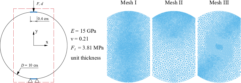
The force-displacement curves are shown in Figure 7. From the results it can be found:
- 1.
When , the stiffness of the structure are generally similar with different ;
- 2.
When , the stiffness of the structure are generally similar with different meshes;
- 3.
The values of the peak load increase considerably with the increasing of ;
- 4.
The values of the peak load are slightly different with different meshes;
- 5.
When , the values of the peak load approach the analytical value.
The final finding coincides with the common assumption used in most PD model using unified grid points that the horizon should be around three times of the spacing of the material points. On the other hand, for specific mesh, though the order of the global stiffness matrix is the same, the computing time will increase with the increasing of , see Figure 8. Because when increases, the global stiffness matrix becomes denser.


Furthermore, we follow the finding that the peak load changes with . Considering the results with Mesh I, we obtain the equivalent tensile strength from , depending on . The results is illustrated in Figure 9 where the fitting curve is
| (22) |

Finally, the damage degree and deformation plots are shown in Figures 10 to 12. Generally similar and reasonable failure patterns are found. The damage initiate from the middle of the disk, but not from the boundary. This is agreeable with the experiments. Moreover, it proves that the boundary weakness of PD model is greatly mitigated in the NHPD.


3.2 Brazilian disk tests with slots
Brazilian disk tests with a single slot and multiple slots were experimentally investigated in HAERI201420, Haeri2015. The models are shown in Figure 13. Mesh I shown in Figure 6 is used. The slots are not explicitly modeled but the bonds intersect with the slots are removed. About the material properties, same values of , , and as taken in the last example are used. On the other hand, we consider different values of . Hence the values of is adjusted based on Eq. 22, as: i) MPa, ii) MPa, and iii) MPa. is used for obtaining normalized peak loads for all cases.
For disk tests with an inclined slot, the force-displacement curves and normalized peak loads are shown in Figure 14, indicating agreeable results comparing to the results provided by phase field method Zhou2019 and Cracking Elements Method Yiming:20. The damage degree and deformation plots considering and are shown in Figures 15 and 16.


For disk tests with multiple slots, the force-displacement curves and normalized peak loads are shown in Figure 17, indicating weak dependency between the results and after using adjusted . The damage degree and deformation plots are shown in Figures 18 to 20, comparing to the experimental results provided in Haeri2015. Generally the patterns of cracking are similar.


3.3 Plate with an inclined slot
Plate made of PMMA with an inclined slot is a benchmark test for PD provided in Pdtheory, which was experimentally investigated in AYATOLLAHI20091563. In the experiments, the cracks propagate axis-symmetrically. The model, material and mesh of the test are shown in Figure 21. The bonds intersect with the slot are removed for implicitly modeling the slot. This strategy inevitably makes the crack tips a little coarse, see Figure 22. This example is used for testing the influences of mesh on crack propagation. There is a refined region on the left side of the model for checking whether the crack will be attracted by this region. Different values of are considered and the values of is adjusted based on Eq. 22, as: i) MPa, ii) MPa, and iii) MPa.
The relationship between the peak loads and the inclined angle is illustrated in Figure 23. Considering different values of , after adjusting , the obtained peak loads are generally similar. The damage degree plots are shown in Figure 24. In most cases, similar to the experiments, axis-symmetrical cracks (damaged regions) are obtained. The crack is not attracted by the refined region on the left side. Some unexpected branches are found in some cases, such as in the case with , , which we attribute mainly to the coarse modeling of the crack tips.


4 Conclusions
In this work, we present a micropolar peridynamics model with non-unified horizon (NHPD). The main features are summarized as
- 1.
In the pre-processing step, normal FEM discretization is used for providing material points. The horizon varies with different points the size of which depends on the shortest distance between neighboring points. The ratio of size of horizon to the shortest distance equals to a prescribed value . When increases, the non-local effects are enhanced;
- 2.
An iterative domain correction strategy is proposed for assuring the equivalence of strain energy density. Then, based on the maximum strain energy density, a novel failure criterion is proposed for the NHPD which bridges the critical stretch to the mechanical strength ;
- 3.
Considering numerical studies regarding different values of and different meshes, the results indicate NHPD shows generally weak mesh dependency. Moreover, it is found that if , has weak influences on the stiffness of the structure while has great influence on the equivalent strength of the structure . A linear relationship between and is obtained and when ;
- 4.
Considering the linear relationship between and then adjusting the inputed , similar results can be obtained regarding different values of .
The NHPD shows another routine for developing peridynamics models and the relationship between equivalent strength and indicates correlations between strength and local/non-local damages.
5 Acknowledgement
The authors gratefully acknowledge financial support by the National Natural Science Foundation of China (NSFC) (51809069) and by the Hebei Province Natural Science Fund E2019202441 and the 2019 Foreign Experts Plan of Hebei Province.
References
- [1] P. Areias, J. Reinoso, P. Camanho, and T. Rabczuk, “A constitutive-based element-by-element crack propagation algorithm with local mesh refinement,” Computational Mechanics, vol. 56, pp. 291–315, 2015.
- [2] P. Areias, T. Rabczuk, and D. Dias-da-Costa, “Element-wise fracture algorithm based on rotation of edges,” Engineering Fracture Mechanics, vol. 110, pp. 113–137, 2013.
- [3] E. C. Mejia Sanchez, L. F. Paullo Muñoz, and D. Roehl, “Discrete fracture propagation analysis using a robust combined continuation method,” International Journal of Solids and Structures, vol. 193-194, pp. 405 – 417, 2020.
- [4] H. Zheng and D. Xu, “New strategies for some issues of numerical manifold method in simulation of crack propagation,” International Journal for Numerical Methods in Engineering, vol. 97, pp. 986–1010, 2014.
- [5] Y. Yang, G. Sun, H. Zheng, and X. Fu, “A four-node quadrilateral element fitted to numerical manifold method with continuous nodal stress for crack analysis,” Computers and Structures, vol. 177, pp. 69–82, 2016.
- [6] Z. Wu, H. Sun, and L. N. Y. Wong, “A cohesive element-based numerical manifold method for hydraulic fracturing modelling with voronoi grains,” Rock Mechanics and Rock Engineering, vol. 52, pp. 2335–2359, 2019.
- [7] J.-H. Song, P. Areias, and T. Belytschko, “A method for dynamic crack and shear band propagation with phantom nodes,” International Journal for Numerical Methods in Engineering, vol. 67, pp. 868–893, 2006.
- [8] J.-Y. Wu and F.-B. Li, “An improved stable XFEM (Is-XFEM) with a novel enrichment function for the computational modeling of cohesive cracks,” Computer Methods in Applied Mechanics and Engineering, vol. 295, pp. 77–107, 2015.
- [9] Y. Zhang, R. Lackner, M. Zeiml, and H. Mang, “Strong discontinuity embedded approach with standard SOS formulation: Element formulation, energy-based crack-tracking strategy, and validations,” Computer Methods in Applied Mechanics and Engineering, vol. 287, pp. 335–366, 2015.
- [10] Y. Zhang and X. Zhuang, “Cracking elements: a self-propagating strong discontinuity embedded approach for quasi-brittle fracture,” Finite Elements in Analysis and Design, vol. 144, pp. 84–100, 2018.
- [11] Y. Zhang and H. A. Mang, “Global cracking elements: a novel tool for Galerkin-based approaches simulating quasi-brittle fracture,” International Journal for Numerical Methods in Engineering, vol. 121, pp. 2462–2480, 2020.
- [12] C. Miehe, L.-M. Schänzel, and H. Ulmer, “Phase field modeling of fracture in multi-physics problems. Part I. Balance of crack surface and failure criteria for brittle crack propagation in thermo-elastic solids,” Computer Methods in Applied Mechanics and Engineering, vol. 294, pp. 449–485, 2015.
- [13] J.-Y. Wu and V. P. Nguyen, “A length scale insensitive phase-field damage model for brittle fracture,” Journal of the Mechanics and Physics of Solids, vol. 119, pp. 20–42, 2018.
- [14] J.-Y. Wu, “A unified phase-field theory for the mechanics of damage and quasi-brittle failure,” Journal of the Mechanics and Physics of Solids, vol. 103, pp. 72–99, 2017.
- [15] T. Rabczuk and T. Belytschko, “Cracking particles: a simplified meshfree method for arbitrary evolving cracks,” International Journal for Numerical Methods in Engineering, vol. 61, pp. 2316–2343, 2004.
- [16] T. Rabczuk and T. Belytschko, “A three-dimensional large deformation meshfree method for arbitrary evolving cracks,” Computer Methods in Applied Mechanics and Engineering, vol. 196, pp. 2777–2799, 2007.
- [17] T. Rabczuk, G. Zi, S. Bordas, and H. Nguyen-Xuan, “A simple and robust three-dimensional cracking-particle method without enrichment,” Computer Methods in Applied Mechanics and Engineering, vol. 199, pp. 2437–2455, 2010.
- [18] S. Silling, “Reformulation of elasticity theory for discontinuities and long-range force,” Journal of the Mechanics and Physics of Solids, vol. 48, pp. 175–209, 2000.
- [19] H. Fei and L. Gilles, “Coupling of nonlocal and local continuum models by the arlequin approach,” International Journal for Numerical Methods in Engineering, vol. 89, no. 6, pp. 671–685, 2011.
- [20] D. Han, Y. Zhang, Q. Wang, W. Lu, and B. Jia, “The review of the bond-based peridynamics modeling,” Journal of Micromechanics and Molecular Physics, vol. 04, no. 01, p. 1830001, 2019.
- [21] J. Trageser and P. Seleson, “Bond-based peridynamics: a tale of two poisson’s ratios,” Journal of Peridynamics and Nonlocal Modeling, Apr 2020.
- [22] Q.-Z. Zhu and T. Ni, “Peridynamic formulations enriched with bond rotation effects,” International Journal of Engineering Science, vol. 121, pp. 118–129, 2017.
- [23] W.-J. Li, Q.-Z. Zhu, and T. Ni, “A local strain-based implementation strategy for the extended peridynamic model with bond rotation,” Computer Methods in Applied Mechanics and Engineering, vol. 358, p. 112625, 2020.
- [24] X. Gu and Q. Zhang, “A modified conjugated bond-based peridynamic analysis for impact failure of concrete gravity dam,” Meccanica, vol. 55, pp. 547–566, Mar 2020.
- [25] H. Yu, X. Chen, and Y. Sun, “A generalized bond-based peridynamic model for quasi-brittle materials enriched with bond tension–rotation–shear coupling effects,” Computer Methods in Applied Mechanics and Engineering, vol. 372, p. 113405, 2020.
- [26] G.-F. Zhao, “Developing a four-dimensional lattice spring model for mechanical responses of solids,” Computer Methods in Applied Mechanics and Engineering, vol. 315, pp. 881–895, 2017.
- [27] M. Nikolić, E. Karavelić, A. Ibrahimbegovic, and P. Miščević, “Lattice element models and their peculiarities,” Archives of Computational Methods in Engineering, vol. 25, pp. 753–784, Jul 2018.
- [28] M. A. Bessa, J. T. Foster, T. Belytschko, and W. K. Liu, “A meshfree unification: reproducing kernel peridynamics,” Computational Mechanics, vol. 53, pp. 1251–1264, Jun 2014.
- [29] H. Ren, X. Zhuang, Y. Cai, and T. Rabczuk, “Dual-horizon peridynamics,” International Journal for Numerical Methods in Engineering, vol. 108, pp. 1451–1476, 2016.
- [30] H. Ren, X. Zhuang, and T. Rabczuk, “Dual-horizon peridynamics: A stable solution to varying horizons,” Computer Methods in Applied Mechanics and Engineering, vol. 318, pp. 762–782, 2017.
- [31] V. Diana and S. Casolo, “A bond-based micropolar peridynamic model with shear deformability: Elasticity, failure properties and initial yield domains,” International Journal of Solids and Structures, vol. 160, pp. 201 – 231, 2019.
- [32] V. Diana and S. Casolo, “A full orthotropic micropolar peridynamic formulation for linearly elastic solids,” International Journal of Mechanical Sciences, vol. 160, pp. 140 – 155, 2019.
- [33] C. Geuzaine and J.-F. Remacle, “Gmsh: A 3-d finite element mesh generator with built-in pre- and post-processing facilities,” International Journal for Numerical Methods in Engineering, vol. 79, no. 11, pp. 1309–1331, 2009.
- [34] E. Madenci and E. Oterkus, Peridynamic theory and its applications. Springer, 2014.
- [35] H. Ren, X. Zhuang, and T. Rabczuk, “Nonlocal operator method with numerical integration for gradient solid,” Computers & Structures, vol. 233, p. 106235, 2020.
- [36] H. Ren, X. Zhuang, and T. Rabczuk, “A higher order nonlocal operator method for solving partial differential equations,” Computer Methods in Applied Mechanics and Engineering, vol. 367, p. 113132, 2020.
- [37] X. Gu, Q. Zhang, and X. Xia, “Voronoi-based peridynamics and cracking analysis with adaptive refinement,” International Journal for Numerical Methods in Engineering, vol. 112, no. 13, pp. 2087–2109, 2017.
- [38] Q. Le and F. Bobaru, “Surface corrections for peridynamic models in elasticity and fracture,” Computational Mechanics, vol. 61, pp. 499–518, 2018.
- [39] D. Yang, X. He, X. Liu, Y. Deng, and X. Huang, “A peridynamics-based cohesive zone model (pd-czm) for predicting cohesive crack propagation,” International Journal of Mechanical Sciences, vol. 184, p. 105830, 2020.
- [40] M. Zaccariotto, F. Luongo, G. sarego, and U. Galvanetto, “Examples of applications of the peridynamic theory to the solution of static equilibrium problems,” The Aeronautical Journal, vol. 119, no. 1216, p. 677–700, 2015.
- [41] J. T. Foster, S. A. Silling, and W. Chen, “An energy based failure criterion for use with peridynamic states,” International Journal for Multiscale Computational Engineering, vol. 9, no. 6, pp. 675–688, 2011.
- [42] D. Huang, G. Lu, and Y. Liu, “Nonlocal peridynamic modeling and simulation on crack propagation in concrete structures,” Mathematical Problems in Engineering, vol. 2015, p. 858723, Feb 2015.
- [43] Y. Zhang and P. Qiao, “A new bond failure criterion for ordinary state-based peridynamic mode II fracture analysis,” International Journal of Fracture, vol. 215, pp. 105–128, Jan 2019.
- [44] D. Dipasquale, G. Sarego, M. Zaccariotto, and U. Galvanetto, “A discussion on failure criteria for ordinary state-based peridynamics,” Engineering Fracture Mechanics, vol. 186, pp. 378 – 398, 2017.
- [45] T. Rabczuk and H. Ren, “A peridynamics formulation for quasi-static fracture and contact in rock,” Engineering Geology, vol. 225, pp. 42–48, 2017.
- [46] V. Diana, J. F. Labuz, and L. Biolzi, “Simulating fracture in rock using a micropolar peridynamic formulation,” Engineering Fracture Mechanics, vol. 230, p. 106985, 2020.
- [47] C. Xu, Y. Yuan, Y. Zhang, and Y. Xue, “Peridynamic modeling of prefabricated beams post-cast with steelfiber reinforced high-strength concrete,” Structural Concrete, vol. n/a, no. n/a.
- [48] Y. Tong, W. Shen, J. Shao, and J. Chen, “A new bond model in peridynamics theory for progressive failure in cohesive brittle materials,” Engineering Fracture Mechanics, vol. 223, p. 106767, 2020.
- [49] Y. Bie, S. Li, X. Hu, and X. Cui, “An implicit dual-based approach to couple peridynamics with classical continuum mechanics,” International Journal for Numerical Methods in Engineering, vol. 120, no. 12, pp. 1349–1379, 2019.
- [50] Y. Zhang and X. Zhuang, “A softening-healing law for self-healing quasi-brittle materials: analyzing with strong discontinuity embedded approach,” Engineering Fracture Mechanics, vol. 192, pp. 290–306, 2018.
- [51] Y. Zhang and X. Zhuang, “Cracking elements method for dynamic brittle fracture,” Theoretical and Applied Fracture Mechanics, vol. 102, pp. 1–9, 2019.
- [52] L. Mu and Y. Zhang, “Cracking elements method with 6-node triangular element,” Finite Elements in Analysis and Design, vol. 177, p. 103421, 2020.
- [53] H. Haeri, K. Shahriar, M. F. Marji, and P. Moarefvand, “Experimental and numerical study of crack propagation and coalescence in pre-cracked rock-like disks,” International Journal of Rock Mechanics and Mining Sciences, vol. 67, pp. 20 – 28, 2014.
- [54] H. Haeri, A. Khaloo, and M. F. Marji, “Experimental and numerical analysis of Brazilian discs with multiple parallel cracks,” Arabian Journal of Geosciences, vol. 8, pp. 5897–5908, 2015.
- [55] S.-W. Zhou and C.-C. Xia, “Propagation and coalescence of quasi-static cracks in Brazilian disks: an insight from a phase field model,” Acta Geotechnica, vol. 14, pp. 1195–1214, Aug 2019.
- [56] M. Ayatollahi and M. Aliha, “Analysis of a new specimen for mixed mode fracture tests on brittle materials,” Engineering Fracture Mechanics, vol. 76, no. 11, pp. 1563 – 1573, 2009.