跳到论文正文
W Papers独立论文阅读器 arXiv:2009.08071 论文正文 计算阅读时间 · 0%
引用这篇论文根据当前论文元数据生成,正式投稿前建议核对。


License: arXiv.org perpetual non-exclusive license
arXiv:2009.08071v2 [math.ST] 22 Apr 2021

Ridge Regression Revisited:
Debiasing, Thresholding and Bootstrap

Yunyi Zhang   and Dimitris N. Politis Thanks: Department of Mathematics, Univ.˜of California–San Diego, La Jolla, CA 92093-0112, USA; yuz334@ucsd.edu Thanks: Department of Mathematics and Halicioglu Data Science Institute, Univ.˜of California–San Diego, La Jolla, CA 92093-0112, USA; dpolitis@ucsd.edu
Abstract

The success of the Lasso in the era of high-dimensional data can be attributed to its conducting an implicit model selection, i.e., zeroing out regression coefficients that are not significant. By contrast, classical ridge regression can not reveal a potential sparsity of parameters, and may also introduce a large bias under the high-dimensional setting. Nevertheless, recent work on the Lasso involves debiasing and thresholding, the latter in order to further enhance the model selection. As a consequence, ridge regression may be worth another look since –after debiasing and thresholding– it may offer some advantages over the Lasso, e.g., it can be easily computed using a closed-form expression. In this paper, we define a debiased and thresholded ridge regression method, and prove a consistency result and a Gaussian approximation theorem. We further introduce a wild bootstrap algorithm to construct confidence regions and perform hypothesis testing for a linear combination of parameters. In addition to estimation, we consider the problem of prediction, and present a novel, hybrid bootstrap algorithm tailored for prediction intervals. Extensive numerical simulations further show that the debiased and thresholded ridge regression has favorable finite sample performance and may be preferable in some settings.

Keywords: Gaussian approximation, high-dimensional data, Lasso, prediction, regression, resampling.

1 Introduction

Linear regression is a fundamental topic in statistical inference. The classical setting assumes the dimension of parameters in a linear model is constant. However, in the modern era, observations may have a comparable or even larger dimension than the number of samples. To perform a consistent estimation with high-dimensional data, statisticians often assume the underlying parameters are sparse (i.e., the parameter vector contains lots of zeros), and proceed with statistical inference based on this assumption.

The success of the Lasso in the setting of high-dimensional data can be attributed to its conducting an implicit model selection, i.e., zeroing out regression coefficients that are not significant; see Tibshirani [1]. More recent work includes: Meinshausen and Bühlmann [2], Meinshausen and Yu [3], and van de Geer [4] for the Lasso estimator’s (model-selection) consistency and applications; Chatterjee and Lahiri [5], [6], Zhang and Cheng [7], and Dezeure et al. [8] for confidence interval construction and hypothesis testing; and Javanmard and Montanari [9], Fan and Li [10], and Chen and Zhou [11] for improvements of the Lasso estimator. Although the Lasso has the desirable property of zeroing out some regression coefficients, van de Geer et al. [12] proposed to further threshold the estimated coefficients, leading to a sparser fitted model. Furthermore, Javanmard and Montanari [13], and Dezeure et al. [8], proposed to debias the Lasso in constructing confidence intervals. See van de Geer [14] and Javanmard and Javadi [15] for recent works of debiased Lasso.

An alternative approach providing consistent estimators for a high dimensional linear model is the so-called post-selection inference. It first applies Lasso to select influential parameters, then fits an ordinary least squares regression on the selected parameters; see Lee et al. [16], Liu and Yu [17], and Tibshirani et al. [18]. We refer to Bühlmann and van de Geer [13] for a comprehensive overview of the Lasso method for high dimensional data.

Ridge regression is a classical method, and its estimator has a closed-form expression, making statistical inference easier than Lasso. However, there is relatively little research on the ridge regression under the high-dimensional setting. Shao and Deng [19] proposed a threshold ridge regression method and proved its consistency. Dai et al. [20] introduced a broken adaptive ridge estimator to approximate L0L_{0} penalized regression. Dobriban and Wager [21] derived the limit of high dimensional ridge regression’s expected predictive risk. Bühlmann [22] used Lasso to correct the bias in a ridge regression estimator, while Lopes [23] applied a residual-based bootstrap to construct confidence intervals.

Three issues have prevented ridge regression from being suitable for a high dimensional linear model:

1. The ridge regression cannot preserve/recover sparsity. Typically, a ridge regression estimator of the parameter vector will not contain any zeros, even though the parameters may be sparse.

2. Bias in the ridge regression estimator can be large. To illustrate this, suppose the parameter of interest is aT​βa^{T}\beta in a linear model y=X​β+ϵy=X\beta+\epsilon; here, the dimension p<np<n (the sample size), XX has rank pp, and aa is a known vector. The ridge estimator is aT​θ~⋆a^{T}\widetilde{\theta}^{\star} with θ~⋆=(XT​X+ρn​Ip)−1​XT​y\widetilde{\theta}^{\star}=(X^{T}X+\rho_{n}I_{p})^{-1}X^{T}y, for some ρn>0\rho_{n}>0, with IpI_{p} denoting the pp-dimensional identity matrix. Performing a thin singular value decomposition X=P​Λ​QTX=P\Lambda Q^{T} (as in Theorem 7.3.2 in Horn and Johnson [24]), and assuming the error vector ϵ\epsilon consists of independent identically distributed (i.i.d.) components, the bias and the standard deviation can be calculated (and controlled) as follows:

𝐄​aT​θ~⋆−aT​β=−ρn​aT​Q​(Λ2+ρn​Ip)−1​QT​β​ which implies ​|𝐄​aT​θ~⋆−aT​β|≤ρn​‖a‖2×‖β‖2λp2+ρn\displaystyle\mathbf{E}a^{T}\widetilde{\theta}^{\star}-a^{T}\beta=-\rho_{n}a^{T}Q(\Lambda^{2}+\rho_{n}I_{p})^{-1}Q^{T}\beta\ \mbox{ which implies }\ |\mathbf{E}a^{T}\widetilde{\theta}^{\star}-a^{T}\beta|\leq\frac{\rho_{n}\|a\|_{2}\times\|\beta\|_{2}}{\lambda^{2}_{p}+\rho_{n}} (1)
and ​V​a​r​(aT​θ~⋆)=V​a​r​(ϵ1)×aT​Q​(Λ2+ρn​Ip)−2​Λ2​QT​a≤V​a​r​(ϵ1)×‖a‖2λp.\displaystyle\mbox{ and }\ \sqrt{Var(a^{T}\widetilde{\theta}^{\star})}=\sqrt{Var(\epsilon_{1})\times a^{T}Q(\Lambda^{2}+\rho_{n}I_{p})^{-2}\Lambda^{2}Q^{T}a}\leq\frac{\sqrt{Var(\epsilon_{1})}\times\|a\|_{2}}{\lambda_{p}}.

In the above, λp\lambda_{p} is the smallest singular value of XX, and ∥⋅∥2\|\cdot\|_{2} is the Euclidean norm of a vector. If ‖β‖2\|\beta\|_{2} does not have a bounded order, the bias may tend to infinity. Another critical problem is that the absolute value of the bias can be significantly larger than the standard deviation, which makes constructing confidence intervals difficult.

3. When the dimension of parameters is larger than the sample size, ridge regression estimates the projection of parameters on the linear space spanned by rows of XX (Shao and Deng [19]). The projection (which can now be considered to be the ‘parameters’ of the linear model) is not sparse, bringing extra burdens for statistical inference.

The third issue comes from the nature of ridge regression, and it is not necessarily bad; our section 6 provides an example to illustrate this. The first two issues can be solved by thresholding and debiasing respectively, yielding an improved ridge regression that will be the focus of this paper. If the Lasso is in need of thresholding and debiasing –as van de Geer et al. [12], Dezeure et al. [8], and Bühlmann and van de Geer [13] seem to suggest– then it loses some of its attractiveness, in which case (improved) ridge regression may be worth another look. If (improved) ridge regression turns out to have comparable performance to threshold Lasso, then the former would be preferable since it can be easily computed using a closed-form expression. Indeed, numerical simulations in section 6 indicate that improved ridge regression has favorable finite-sample performance, and has a further advantage over the Lasso: it is robust against a non-optimal choice of the hyperparameters.

Apart from point estimation using improved ridge regression, this paper presents a Gaussian approximation theorem for the improved ridge regression estimator. Applying this result, we propose a wild bootstrap algorithm to construct a confidence region for γ=M​β\gamma=M\beta with MM a known matrix and/or test the null hypothesis γ=γ0\gamma=\gamma_{0} with γ0\gamma_{0} a known vector, versus the alternative hypothesis γ≠γ0\gamma\neq\gamma_{0}. The wild bootstrap was developed in the 1980s by Wu [25] and Liu [26]; its applicability to high-dimensional problems was recognized early on by Mammen [27]. Here we will use the wild bootstrap in its Gaussian residuals version that has been found useful in high-dimensional regression; see Chernozhukov et al. [28]. Estimating and testing γ\gamma are important problems in econometrics, e.g., Dolado and Lütkepohl [29], Sun [https://urldefense.com/v3/__https://doi.org/10.1111/j.1368-423X.2012.00390.x__;!!Mih3wA!Q9aoQVO8cn4eWInRmrOzFAYeiX19a7xKzrpyC3_noHS-Dc6SZcpIQu17FxU-vidS2g$], [30], and Gonçalves and Vogelsang [31]. Besides, estimating γ\gamma directly contributes to prediction, which is an important topic in modern age statistics.

Finally, we consider statistical prediction based on the improved ridge regression estimator for a high-dimensional linear model. For a regression problem, quantifying a predictor’s accuracy can be as important as predicting accurately. To do that, it is useful to be able to construct a prediction interval to accompany the point prediction; this is usually done by some form of bootstrap; see Stine [32] for a classical result, and Politis [33] for a comprehensive treatment of both model-based and model-free prediction intervals in regression. As an alternative to the bootstrap, conformal prediction may be a tool to yield prediction intervals; see e.g. Romano et al. [34] and Romano et al. [35]. In our point of view, however, the bootstrap is preferable as it captures the underlying variability of estimated quantities; Section 5 in what follows gives the details.

The remainder of this paper is organized as follows: Section 2 introduces frequently used notations and assumptions. Section 3 presents the consistency result and the Gaussian approximation theorem for the improved ridge regression estimator. Section 4 constructs a confidence region for γ=M​β\gamma=M\beta, and tests the null hypothesis γ=γ0\gamma=\gamma_{0} versus the alternative hypothesis γ≠γ0\gamma\neq\gamma_{0} via a bootstrap algorithm. Section 5 constructs bootstrap prediction intervals in our ridge regression setting using a novel, hybrid resampling procedure. Finally, Section 6 provides extensive simulations to illustrate the finite sample performance, while Section 7 gives some concluding remarks; technical proofs are deferred to the Appendix.

2 Preliminaries

Our work focuses on the fixed design linear model

y=X​β+ϵy=X\beta+\epsilon (2)

where the (unknown) parameter vector β\beta is pp-dimensional, and the n×pn\times p fixed (nonrandom) design matrix XX is assumed to have rank rr. Define the known matrix of linear combination coefficients as M=(mi​j)i=1,2,…,p1,j=1,2,…,pM=(m_{ij})_{i=1,2,...,p_{1},j=1,2,...,p} so that MM has p1p_{1} rows. The linear combination of interest are γ=(γ1,…,γp1)T=M​β\gamma=(\gamma_{1},...,\gamma_{p_{1}})^{T}=M\beta.

Perform a thin singular value decomposition X=P​Λ​QTX=P\Lambda Q^{T} as in Theorem 7.3.2 in Horn and Johnson [24]; here, PP and QQ respectively is n×rn\times r and p×rp\times r orthonormal matrices that satisfy PT​P=QT​Q=IrP^{T}P=Q^{T}Q=I_{r}, where IrI_{r} denotes the r×rr\times r identity matrix. Furthermore, Λ=d​i​a​g​(λ1,…,λr)\Lambda=diag(\lambda_{1},...,\lambda_{r}), and λ1≥λ2≥…≥λr>0\lambda_{1}\geq\lambda_{2}\geq...\geq\lambda_{r}>0 are positive singular values of XX.

Denote Q⟂Q_{\perp} as the p×(p−r)p\times(p-r) orthonormal complement of QQ; then we have

Q⟂T​Q⟂=Ip−r,QT​Q⟂=0,and ​Q​QT+Q⟂​Q⟂T=Ip;Q_{\perp}^{T}Q_{\perp}=I_{p-r},\ Q^{T}Q_{\perp}=0,\ \text{and }QQ^{T}+Q_{\perp}Q_{\perp}^{T}=I_{p}; (3)

in the above, 00 is the r×(p−r)r\times(p-r) matrix having all elements 00. Define ζ=QT​β\zeta=Q^{T}\beta and θ=(θ1,…,θp)T=Q​ζ=Q​QT​β\theta=(\theta_{1},...,\theta_{p})^{T}=Q\zeta=QQ^{T}\beta, then X​β=X​θX\beta=X\theta, θT​θ=ζT​QT​Q​ζ=ζT​ζ\theta^{T}\theta=\zeta^{T}Q^{T}Q\zeta=\zeta^{T}\zeta. According to Shao and Deng [19], the ridge regression estimates θ\theta rather than β\beta.

Define θ⟂=Q⟂​Q⟂T​β\theta_{\perp}=Q_{\perp}Q_{\perp}^{T}\beta, so β=θ+θ⟂\beta=\theta+\theta_{\perp}. If the design matrix XX has rank p≤np\leq n, then Q⟂Q_{\perp} does not exist. In this situation, we define θ⟂=0\theta_{\perp}=0, the pp dimensional vector with all elements 00. For a threshold bnb_{n}, define the set 𝒩bn={i||θi|>bn}\mathcal{N}_{b_{n}}=\{i\ ||\theta_{i}|>b_{n}\}. After selecting a suitable bnb_{n}, define

ci​k=∑j∈𝒩bnmi​jqj​k,∀i=1,2,…,p1,k=1,2,…,r,and ℳ={i|∑k=1rci​k2>0}c_{ik}=\sum_{j\in\mathcal{N}_{b_{n}}}m_{ij}q_{jk},\ \forall\ i=1,2,...,p_{1},\ k=1,2,...,r,\ \text{and }\mathcal{M}=\{i\ |\sum_{k=1}^{r}c_{ik}^{2}>0\} (4)

Define τi,i=1,2,…,p1\tau_{i},\ i=1,2,...,p_{1} as

τi=∑k=1rci​k2​(λkλk2+ρn+ρn​λk(λk2+ρn)2)2+1n\displaystyle\tau_{i}=\sqrt{\sum_{k=1}^{r}c_{ik}^{2}\left(\frac{\lambda_{k}}{\lambda_{k}^{2}+\rho_{n}}+\frac{\rho_{n}\lambda_{k}}{(\lambda_{k}^{2}+\rho_{n})^{2}}\right)^{2}+\frac{1}{n}} (5)

We will use the standard order notations O⁡(⋅),o⁡(⋅),Op​(⋅),O(\cdot),\ o(\cdot),\ O_{p}(\cdot), and op​(⋅)o_{p}(\cdot). For two numerical sequences an,bn,n=1,2,…a_{n},b_{n},n=1,2,..., we say an=O⁡(bn)a_{n}=O(b_{n}) if ∃\exists a constant C>0C>0 such that |an|≤C​|bn||a_{n}|\leq C|b_{n}| for all nn, and an=o⁡(bn)a_{n}=o(b_{n}) if limn→∞anbn=0\lim_{n\to\infty}\frac{a_{n}}{b_{n}}=0. For two random variable sequences Xn,YnX_{n},Y_{n}, we say Xn=Op​(Yn)X_{n}=O_{p}(Y_{n}) if for any 0<ϵ<10<\epsilon<1, ∃\exists a constant Cϵ>0C_{\epsilon}>0 such that supnP​r​o​b​(|Xn|≥Cϵ​|Yn|)≤ϵ\sup_{n}Prob(|X_{n}|\geq C_{\epsilon}|Y_{n}|)\leq\epsilon; and Xn=op​(Yn)X_{n}=o_{p}(Y_{n}) if XnYn→p0\frac{X_{n}}{Y_{n}}\to_{p}0; see e.g. Definition 1.9 and Chapter 1.5.1 of Shao [36]. All order notations and convergences in this paper will be understood to hold as the sample size n→∞n\to\infty.

For a finite set AA, |A||A| denotes the number of elements in AA. Notations ∃\exists and ∀\forall denote “there exists” and “for all” respectively. P​r​o​b∗​(⋅)Prob^{*}\left(\cdot\right) and 𝐄∗⋅\mathbf{E}^{*}\cdot respectively represent probability and expectation in the “bootstrap world”, i.e., they are the conditional probability Prob(⋅|y)Prob(\cdot|y) and the conditional expectation 𝐄(⋅|y)\mathbf{E}(\cdot|y).

Suppose H⁡(x)H(x) is a cumulative distribution function and 0<α<10<\alpha<1; then the 1−α1-\alpha quantile of HH is defined as

c1−α=inf{x∈𝐑|H⁡(x)≥1−α}.c_{1-\alpha}=\inf\{x\in\mathbf{R}|H(x)\geq 1-\alpha\}. (6)

In particular, given some order statistics X1≤X2≤…≤XBX_{1}\leq X_{2}\leq...\leq X_{B}, the 1−α1-\alpha sample quantile C1−αC_{1-\alpha} is defined as

C1−α=Xi∗such that ​i∗=min⁡{i|1B​∑j=1B𝟏Xj≤Xi≥1−α}.C_{1-\alpha}=X_{i_{*}}\ \ \text{such that }i_{*}=\min\left\{i\ \Big|\ \frac{1}{B}\sum_{j=1}^{B}\mathbf{1}_{X_{j}\leq X_{i}}\geq 1-\alpha\right\}. (7)

Other notations will be defined before being used. Without being explicitly specified, the convergence results in this paper assume the sample size n→∞n\to\infty.

The high dimensionality in this paper comes from two aspects: the number of parameters pp may increase with the sample size nn, and (for statistical inference/hypothesis testing) the number of simultaneous linear combinations p1p_{1} and |ℳ||\mathcal{M}| can also increase with nn.

Our work adopts the following assumptions:

Assumptions

1. Assume a fixed design, i.e., the design matrix XX is deterministic. Also assume that there exist constants cλ,Cλ>0c_{\lambda},C_{\lambda}>0, 0<η≤1/20<\eta\leq 1/2, such that the positive singular values of XX satisfy

Cλ​n1/2≥λ1≥λ2≥…≥λr≥cλ​nη.C_{\lambda}n^{1/2}\geq\lambda_{1}\geq\lambda_{2}\geq...\geq\lambda_{r}\geq c_{\lambda}n^{\eta}. (8)

Furthermore, the Euclidean norm of θ\theta is assumed to satisfy ‖θ‖2=∑i=1pθi2=O⁡(nαθ)\|\theta\|_{2}=\sqrt{\sum_{i=1}^{p}\theta_{i}^{2}}=O(n^{\alpha_{\theta}}) with 0<αθ<3​η0<\alpha_{\theta}<3\eta.

2. The ridge parameter satisfies ρn=O⁡(n2​η−δ)\rho_{n}=O(n^{2\eta-\delta}) with a positive constant δ\delta such that η+αθ2<δ<2​η\frac{\eta+\alpha_{\theta}}{2}<\delta<2\eta

3. The errors ϵ=(ϵ1,…,ϵn)T\epsilon=(\epsilon_{1},...,\epsilon_{n})^{T} driving regression (2) are assumed to be i.i.d., with 𝐄​ϵ1=0\mathbf{E}\epsilon_{1}=0, and 𝐄​|ϵ1|m<∞\mathbf{E}|\epsilon_{1}|^{m}<\infty for some m>4m>4.

4. The dimension of the parameter vector β\beta satisfies p=O⁡(nαp)p=O(n^{\alpha_{p}}) for some constant αp∈[0,m​η)\alpha_{p}\in[0,m\eta) where m,ηm,\eta are as defined in Assumptions 1–3. Furthermore, the threshold bnb_{n} is chosen as bn=Cb×n−νbb_{n}=C_{b}\times n^{-\nu_{b}} with constants Cb,νb>0C_{b},\nu_{b}>0 and νb+αpm−η<0\nu_{b}+\frac{\alpha_{p}}{m}-\eta<0. We assume ∃\exists a constant 0<cb<10<c_{b}<1 such that maxi∉𝒩bn⁡|θi|≤cb×bn\max_{i\not\in\mathcal{N}_{b_{n}}}|\theta_{i}|\leq c_{b}\times b_{n}, and mini∈𝒩bn⁡|θi|≥bncb\min_{i\in\mathcal{N}_{b_{n}}}|\theta_{i}|\geq\frac{b_{n}}{c_{b}}.

5. ℳ\mathcal{M} (defined in (4)) is not empty and |ℳ|=O⁡(nαℳ)|\mathcal{M}|=O(n^{\alpha_{\mathcal{M}}}) with αℳ<m​η\alpha_{\mathcal{M}}<m\eta where m,ηm,\eta are as defined in Assumptions 1–3. Besides, assume ∃\exists constants cℳ,Cℳc_{\mathcal{M}},C_{\mathcal{M}} such that 0<cℳ<∑k=1rci​k2≤Cℳ0<c_{\mathcal{M}}<\sum_{k=1}^{r}c_{ik}^{2}\leq C_{\mathcal{M}} for all i∈ℳi\in\mathcal{M}. Also assume

maxi=1,2,…,p1⁡|∑j∉𝒩bnmi​j​θj|=o⁡(1n​log⁡(n))​and​maxi=1,2,…,p1|∑j=1pmi​j​θ⟂,j|=o⁡(1n​log⁡(n))\max_{i=1,2,...,p_{1}}|\sum_{j\not\in\mathcal{N}_{b_{n}}}m_{ij}\theta_{j}|=o\left(\frac{1}{\sqrt{n\log(n)}}\right)\ \text{and}\ \max_{i=1,2,...,p_{1}}|\sum_{j=1}^{p}m_{ij}\theta_{\perp,j}|=o\left(\frac{1}{\sqrt{n\log(n)}}\right) (9)

6. ∃\exists a constant ασ\alpha_{\sigma} satisfying η≥ασ>0\eta\geq\alpha_{\sigma}>0 such that

n−νb​∑j∉𝒩bn|θj|=O⁡(n−ασ),|𝒩bn|nη=O⁡(n−ασ)n^{-\nu_{b}}\sum_{j\not\in\mathcal{N}_{b_{n}}}|\theta_{j}|=O(n^{-\alpha_{\sigma}}),\ \ \frac{\sqrt{|\mathcal{N}_{b_{n}}|}}{n^{\eta}}=O(n^{-\alpha_{\sigma}}) (10)

7. |ℳ|≤r|\mathcal{M}|\leq r, the matrix T=(ci​k)i∈ℳ,k=1,2,…,rT=(c_{ik})_{i\in\mathcal{M},k=1,2,...,r} has rank |ℳ||\mathcal{M}|, and one of the two following conditions holds true:

7.1.

maxi∈ℳ,l=1,2,…,n|1τi×∑k=1rci​kpl​k(λkλk2+ρn+ρn​λk(λk2+ρn)2)|=o(min(n(ασ−1)/2×log−3/2(n),n−1/3×log−3/2(n))\max_{i\in\mathcal{M},l=1,2,...,n}|\frac{1}{\tau_{i}}\times\sum_{k=1}^{r}c_{ik}p_{lk}\left(\frac{\lambda_{k}}{\lambda_{k}^{2}+\rho_{n}}+\frac{\rho_{n}\lambda_{k}}{(\lambda_{k}^{2}+\rho_{n})^{2}}\right)|=o(\min(n^{(\alpha_{\sigma}-1)/2}\times\log^{-3/2}(n),\ n^{-1/3}\times\log^{-3/2}(n)) (11)

7.2. ασ<1/2\alpha_{\sigma}<1/2 and

|ℳ|=o⁡(nασ×log−3⁡(n))\displaystyle|\mathcal{M}|=o(n^{\alpha_{\sigma}}\times\log^{-3}(n)) (12)
maxi∈ℳ,l=1,2,…,n|1τi×∑k=1rci​kpl​k(λkλk2+ρn+ρn​λk(λk2+ρn)2)|=O(n−ασ×log−3/2(n))\displaystyle\max_{i\in\mathcal{M},l=1,2,...,n}|\frac{1}{\tau_{i}}\times\sum_{k=1}^{r}c_{ik}p_{lk}\left(\frac{\lambda_{k}}{\lambda_{k}^{2}+\rho_{n}}+\frac{\rho_{n}\lambda_{k}}{(\lambda_{k}^{2}+\rho_{n})^{2}}\right)|=O(n^{-\alpha_{\sigma}}\times\log^{-3/2}(n))
Remark 1

The intuitive meaning of assumption 4 is that the θi\theta_{i}s that are not being truncated should be significantly larger than the θi\theta_{i} being truncated. Furthermore, note that

∑l=1n(∑k=1rci​k​pl​k​(λkλk2+ρn+ρn​λk(λk2+ρn)2))2=∑k=1rci​k2​(λkλk2+ρn+ρn​λk(λ2+ρn)2)2≤τi2.\sum_{l=1}^{n}\left(\sum_{k=1}^{r}c_{ik}p_{lk}\left(\frac{\lambda_{k}}{\lambda_{k}^{2}+\rho_{n}}+\frac{\rho_{n}\lambda_{k}}{(\lambda_{k}^{2}+\rho_{n})^{2}}\right)\right)^{2}=\sum_{k=1}^{r}c^{2}_{ik}\left(\frac{\lambda_{k}}{\lambda^{2}_{k}+\rho_{n}}+\frac{\rho_{n}\lambda_{k}}{(\lambda^{2}+\rho_{n})^{2}}\right)^{2}\leq\tau^{2}_{i}. (13)

Therefore, assumption 7 implies that no single element in the matrix (1τi​∑k=1rci​k​pl​k​(λkλk2+ρn+ρn​λk(λk2+ρn)2))i∈ℳ,l=1,…,n\left(\frac{1}{\tau_{i}}\sum_{k=1}^{r}c_{ik}p_{lk}\left(\frac{\lambda_{k}}{\lambda_{k}^{2}+\rho_{n}}+\frac{\rho_{n}\lambda_{k}}{(\lambda_{k}^{2}+\rho_{n})^{2}}\right)\right)_{i\in\mathcal{M},l=1,...,n} dominates the others. We use τi,i=1,…,p1\tau_{i},i=1,...,p_{1} to prevent the normalizing parameters from being 00. We do not require that the design matrix has rank min⁡(n,p)\min(n,p) or that p<np<n. However, when these conditions are not satisfied, the sparsity of θ\theta, i.e., assumption 6, can be violated. Section 6 uses a numerical simulation to illustrate this problem.

3 Consistency and the Gaussian approximation theorem

Throughout, we will use the notations developed in section 2. For a chosen ridge parameter ρn>0\rho_{n}>0, define the classical ridge regression estimator θ~⋆\widetilde{\theta}^{\star} and the de-biased estimator θ~\widetilde{\theta} as

θ~⋆=(XT​X+ρn​Ip)−1​XT​y\displaystyle\widetilde{\theta}^{\star}=(X^{T}X+\rho_{n}I_{p})^{-1}X^{T}y (14)
θ~=(θ~1,…,θ~p)T=θ~⋆+ρn×Q​(Λ2+ρn​Ir)−1​QT​θ~⋆\displaystyle\widetilde{\theta}=(\widetilde{\theta}_{1},...,\widetilde{\theta}_{p})^{T}=\widetilde{\theta}^{\star}+\rho_{n}\times Q(\Lambda^{2}+\rho_{n}I_{r})^{-1}Q^{T}\widetilde{\theta}^{\star}

Then we have

θ~−θ=−ρn2​Q​(Λ2+ρn​Ir)−2​ζ+Q⁡((Λ2+ρn​Ir)−1​Λ+ρn​(Λ2+ρn​Ir)−2​Λ)​PT​ϵ\displaystyle\widetilde{\theta}-\theta=-\rho_{n}^{2}Q(\Lambda^{2}+\rho_{n}I_{r})^{-2}\zeta+Q\left((\Lambda^{2}+\rho_{n}I_{r})^{-1}\Lambda+\rho_{n}(\Lambda^{2}+\rho_{n}I_{r})^{-2}\Lambda\right)P^{T}\epsilon (15)

Similar to 𝒩bn\mathcal{N}_{b_{n}}, define the set 𝒩^bn\widehat{\mathcal{N}}_{b_{n}}, the estimator θ^=(θ^1,…,θ^p)T\widehat{\theta}=(\widehat{\theta}_{1},...,\widehat{\theta}_{p})^{T} and γ^\widehat{\gamma} as

𝒩^bn={i||θ~i|>bn},θ^i=θ~i×𝟏i∈𝒩^bn,γ^=M​θ^\widehat{\mathcal{N}}_{b_{n}}=\left\{i\ \Big||\widetilde{\theta}_{i}|>b_{n}\right\},\ \ \widehat{\theta}_{i}=\widetilde{\theta}_{i}\times\mathbf{1}_{i\in\widehat{\mathcal{N}}_{b_{n}}},\ \ \widehat{\gamma}=M\widehat{\theta} (16)

Then, θ^\widehat{\theta} and γ^\widehat{\gamma} constitute the improved, i.e., debiased and thresholded, ridge regression estimator for the parameter vector θ\theta and γ=M​β\gamma=M\beta respectively. Apart from parameter estimation, we need to estimate the error variance σ2=𝐄​ϵ12\sigma^{2}=\mathbf{E}\epsilon^{2}_{1}. The estimator for σ2\sigma^{2} is

σ^2=1n​∑i=1n(yi−∑j=1pxi​j​θ^j)2\widehat{\sigma}^{2}=\frac{1}{n}\sum_{i=1}^{n}(y_{i}-\sum_{j=1}^{p}x_{ij}\widehat{\theta}_{j})^{2} (17)
Theorem 1

1. Suppose assumptions 1 to 5 hold true. Then

P​r​o​b​(𝒩^bn≠𝒩bn)=O⁡(nαp+m​νb−m​η)and ​maxi=1,2,…,p1​|γ^i−γi|=Op​(|ℳ|1/m×n−η)Prob\left(\widehat{\mathcal{N}}_{b_{n}}\neq\mathcal{N}_{b_{n}}\right)=O(n^{\alpha_{p}+m\nu_{b}-m\eta})\ \ \text{and }\max_{i=1,2,...,p_{1}}|\widehat{\gamma}_{i}-\gamma_{i}|=O_{p}(|\mathcal{M}|^{1/m}\times n^{-\eta}) (18)

where γi,i=1,…,p1\gamma_{i},i=1,...,p_{1} and 𝒩bn\mathcal{N}_{b_{n}} are defined in section 2.

2. Suppose assumptions 1 to 6 hold true. Then

|σ^2−σ2|=Op​(n−ασ).|\widehat{\sigma}^{2}-\sigma^{2}|=O_{p}(n^{-\alpha_{\sigma}}). (19)

Define τ^i,i=1,2,…,p1\widehat{\tau}_{i},\ i=1,2,...,p_{1} and H⁡(x),x∈𝐑H(x),x\in\mathbf{R} as

τ^i=∑k=1r(∑j∈𝒩^bnmi​j​qj​k)2×(λkλk2+ρn+ρn​λk(λk2+ρn)2)2+1n\displaystyle\widehat{\tau}_{i}=\sqrt{\sum_{k=1}^{r}\left(\sum_{j\in\widehat{\mathcal{N}}_{b_{n}}}m_{ij}q_{jk}\right)^{2}\times\left(\frac{\lambda_{k}}{\lambda_{k}^{2}+\rho_{n}}+\frac{\rho_{n}\lambda_{k}}{(\lambda_{k}^{2}+\rho_{n})^{2}}\right)^{2}+\frac{1}{n}} (20)
H⁡(x)=P​r​o​b​(maxi∈ℳ⁡1τi​|∑k=1rci​k​(λkλk2+ρn+ρn​λk(λk2+ρn)2)​ξk|≤x)\displaystyle H(x)=Prob\left(\max_{i\in\mathcal{M}}\frac{1}{\tau_{i}}|\sum_{k=1}^{r}c_{ik}\left(\frac{\lambda_{k}}{\lambda_{k}^{2}+\rho_{n}}+\frac{\rho_{n}\lambda_{k}}{(\lambda_{k}^{2}+\rho_{n})^{2}}\right)\xi_{k}|\leq x\right)
Here ξk,k=1,2,…,r are independent normal random variables with mean 0 and variance σ2=𝐄​ϵ12.\displaystyle\text{Here $\xi_{k},\ k=1,2,...,r$ are independent normal random variables with mean $0$ and variance $\sigma^{2}=\mathbf{E}\epsilon_{1}^{2}$. }

|ℳ||\mathcal{M}| (defined in (4)) and p1p_{1} may grow as the sample size increases. In this case, the estimator maxi=1,2,…,p1⁡|γ^i−γi|τ^i\max_{i=1,2,...,p_{1}}\frac{|\widehat{\gamma}_{i}-\gamma_{i}|}{\widehat{\tau}_{i}} does not have an asymptotic distribution. However, the cumulative distribution function of maxi=1,2,…,p1⁡|γ^i−γi|τ^i\max_{i=1,2,...,p_{1}}\frac{|\widehat{\gamma}_{i}-\gamma_{i}|}{\widehat{\tau}_{i}} still can be approximated by H⁡(x)H(x) (whose expression changes as the sample size increases as well). Define c1−αc_{1-\alpha} as the 1−α1-\alpha quantile of HH; theorem 2 implies that the set

{γ=(γ1,…,γp1)|maxi=1,…,p1⁡|γ^i−γi|τ^i≤c1−α}\left\{\gamma=(\gamma_{1},...,\gamma_{p_{1}})\Big|\max_{i=1,...,p_{1}}\frac{|\widehat{\gamma}_{i}-\gamma_{i}|}{\widehat{\tau}_{i}}\leq c_{1-\alpha}\right\} (21)

is an asymptotically valid (1−α)×100(1-\alpha)\times 100% confidence region for the parameter of interest γ\gamma.

Theorem 2

Suppose assumptions 1 to 7 hold true. Then

limn→∞supx≥0|P​r​o​b​(maxi=1,2,…,p1⁡|γ^i−γi|τ^i≤x)−H⁡(x)|=0\lim_{n\to\infty}\sup_{x\geq 0}|Prob\left(\max_{i=1,2,...,p_{1}}\frac{|\widehat{\gamma}_{i}-\gamma_{i}|}{\widehat{\tau}_{i}}\leq x\right)-H(x)|=0 (22)

where γi,i=1,…,p1\gamma_{i},i=1,...,p_{1} are defined in section 2.

Gaussian approximation theorems like theorem 2 are useful tools not only in linear models but also in other high dimensional statistics; e.g., Chernozhukov et al. [28] and Zhang and Wu [37].

4 Bootstrap inference and hypothesis testing

An obstacle for constructing a practical confidence region or testing a hypothesis via theorem 2 are the unknown ℳ\mathcal{M}, 𝒩bn\mathcal{N}_{b_{n}}, and σ\sigma. Besides, HH is too complicated to have a closed-form formula. Fortunately, statisticians can simulate normal random variables on a computer, so they may use Monte-Carlo simulations to find the 1−α1-\alpha quantile of HH. Based on this idea, this section develops a wild bootstrap algorithm similar to Mammen [27] and Chernozhukov et al. [28] for the following tasks: constructing the confidence region for the parameter of interest γ=M​β\gamma=M\beta; and testing the null hypothesis γ=γ0\gamma=\gamma_{0} (for a known γ0\gamma_{0}) versus the alternative hypothesis γ≠γ0\gamma\neq\gamma_{0}. Similar to Zhang and Cheng [7], Chernozhukov et al. [28], and Zhang and Wu [37], we use the maximum statistic maxi=1,2,…,p1⁡|γ^i−γi|τ^i\max_{i=1,2,...,p_{1}}\frac{|\widehat{\gamma}_{i}-\gamma_{i}|}{\widehat{\tau}_{i}} to construct a simultaneous confidence region.

Algorithm 1 (Wild bootstrap inference and hypothesis testing)

Input: Design matrix XX, dependent variables y=X​β+ϵy=X\beta+\epsilon, linear combination matrix MM, ridge parameter ρn\rho_{n}, threshold bnb_{n}, nominal coverage probability 1−α1-\alpha, number of bootstrap replicates BB

Additional input for testing: γ0=(γ0,1,…,γ0,p1)T\gamma_{0}=(\gamma_{0,1},...,\gamma_{0,p_{1}})^{T}

1. Calculate θ^,γ^=(γ^1,…,γ^p1)T\widehat{\theta},\ \widehat{\gamma}=(\widehat{\gamma}_{1},...,\widehat{\gamma}_{p_{1}})^{T} defined in (16), τ^i,i=1,2,…,p1\widehat{\tau}_{i},\ i=1,2,...,p_{1} defined in (20), and σ^\widehat{\sigma} defined in (17).

2. Generate i.i.d. errors ϵ∗=(ϵ1∗,…,ϵn∗)T\epsilon^{*}=(\epsilon^{*}_{1},...,\epsilon^{*}_{n})^{T} with ϵi∗,i=1,…,n\epsilon^{*}_{i},i=1,...,n having normal distribution with mean 00 and variance σ^2\widehat{\sigma}^{2}, then calculate y∗=X​θ^+ϵ∗y^{*}=X\widehat{\theta}+\epsilon^{*} and θ^⟂=Q⟂​Q⟂T​θ^\widehat{\theta}_{\perp}=Q_{\perp}Q_{\perp}^{T}\widehat{\theta} (Q⟂Q_{\perp} is defined in section 2).

3. Calculate θ~⋆⁣∗=(XT​X+ρn​Ip)−1​XT​y∗\widetilde{\theta}^{\star*}=(X^{T}X+\rho_{n}I_{p})^{-1}X^{T}y^{*} and θ~∗=(θ~1∗,…,θ~p∗)T=θ~⋆⁣∗+ρn×Q​(Λ2+ρn​Ir)−1​QT​θ~⋆⁣∗+θ^⟂\widetilde{\theta}^{*}=(\widetilde{\theta}^{*}_{1},...,\widetilde{\theta}^{*}_{p})^{T}=\widetilde{\theta}^{\star*}+\rho_{n}\times Q(\Lambda^{2}+\rho_{n}I_{r})^{-1}Q^{T}\widetilde{\theta}^{\star*}+\widehat{\theta}_{\perp}.

4. Calculate 𝒩^bn∗={i||θ~i∗|>bn}\widehat{\mathcal{N}}_{b_{n}}^{*}=\left\{i\Big||\widetilde{\theta}_{i}^{*}|>b_{n}\right\} and θ^∗=(θ^1∗,…,θ^p∗)T\widehat{\theta}^{*}=(\widehat{\theta}_{1}^{*},...,\widehat{\theta}_{p}^{*})^{T} with θ^i∗=θ~i∗×𝟏i∈𝒩^bn∗\widehat{\theta}_{i}^{*}=\widetilde{\theta}_{i}^{*}\times\mathbf{1}_{i\in\widehat{\mathcal{N}}^{*}_{b_{n}}} for i=1,2,…,pi=1,2,...,p.

5. Calculate γ^∗=M​θ^∗\widehat{\gamma}^{*}=M\widehat{\theta}^{*}, τ^i∗,i=1,2,…,p1\widehat{\tau}_{i}^{*},i=1,2,...,p_{1}, and Eb∗E_{b}^{*} such that

τ^i∗=∑k=1r(∑j∈𝒩^bn∗mi​j​qj​k)2×(λkλk2+ρn+ρn​λk(λk2+ρn)2)2+1n,Eb∗=maxi=1,2,…,p1⁡|γ^i∗−γ^i|τ^i∗\widehat{\tau}_{i}^{*}=\sqrt{\sum_{k=1}^{r}\left(\sum_{j\in\widehat{\mathcal{N}}^{*}_{b_{n}}}m_{ij}q_{jk}\right)^{2}\times\left(\frac{\lambda_{k}}{\lambda_{k}^{2}+\rho_{n}}+\frac{\rho_{n}\lambda_{k}}{(\lambda_{k}^{2}+\rho_{n})^{2}}\right)^{2}+\frac{1}{n}},\ \ E_{b}^{*}=\max_{i=1,2,...,p_{1}}\frac{|\widehat{\gamma}^{*}_{i}-\widehat{\gamma}_{i}|}{\widehat{\tau}_{i}^{*}} (23)

6.a (For constructing a confidence region) Repeat steps 2 to 5 for BB times to generate Eb∗,b=1,2,…,BE^{*}_{b},\ b=1,2,...,B; then calculate the 1−α1-\alpha sample quantile C1−α∗C^{*}_{1-\alpha} of Eb∗E^{*}_{b}. The 1−α1-\alpha confidence region for the parameter of interest γ=M​β\gamma=M\beta is given by the set

{γ=(γ1,…,γp1)T|maxi=1,2,…,p1⁡|γ^i−γi|τ^i≤C1−α∗}\left\{\gamma=(\gamma_{1},...,\gamma_{p_{1}})^{T}\Big|\max_{i=1,2,...,p_{1}}\frac{|\widehat{\gamma}_{i}-\gamma_{i}|}{\widehat{\tau}_{i}}\leq C^{*}_{1-\alpha}\right\} (24)

6.b (For hypothesis testing) Repeat steps 2 to 5 for BB times to generate Eb∗,b=1,2,…,BE^{*}_{b},\ b=1,2,...,B; then calculate the 1−α1-\alpha sample quantile C1−α∗C^{*}_{1-\alpha} of Eb∗E^{*}_{b}. Reject the null hypothesis γ=γ0\gamma=\gamma_{0} when

maxi=1,2,…,p1⁡|γ^i−γ0,i|τ^i>C1−α∗.\max_{i=1,2,...,p_{1}}\frac{|\widehat{\gamma}_{i}-\gamma_{0,i}|}{\widehat{\tau}_{i}}>C^{*}_{1-\alpha}. (25)

As in section 2, if XX has rank p≤np\leq n, we define θ^⟂=0\widehat{\theta}_{\perp}=0, the pp dimensional vector with all elements 00.

According to theorem 1.2.1 in Politis et al. [38], the consistency of algorithm 25 –either for asymptotic validity of confidence regions or consistency of the hypothesis test– is ensured if

P​r​o​b​(maxi=1,2,…,p1⁡|γ^i−γi|τ^i≤c1−α∗)→1−αProb\left(\max_{i=1,2,...,p_{1}}\frac{|\widehat{\gamma}_{i}-\gamma_{i}|}{\widehat{\tau}_{i}}\leq c^{*}_{1-\alpha}\right)\to 1-\alpha (26)

where c1−α∗c^{*}_{1-\alpha} is the 1−α1-\alpha quantile of the conditional distribution P​r​o​b∗​(maxi=1,2,…,p1⁡|γ^i∗−γ^i|τ^i∗≤x)Prob^{*}\left(\max_{i=1,2,...,p_{1}}\frac{|\widehat{\gamma}^{*}_{i}-\widehat{\gamma}_{i}|}{\widehat{\tau}_{i}^{*}}\leq x\right); we prove this in theorem 3 below.

Theorem 3

Suppose assumptions 1 to 7 hold true. Then

supx≥0|P​r​o​b∗​(maxi=1,2,…,p1⁡|γ^i∗−γ^i|τ^i∗≤x)−H⁡(x)|=oP​(1).\sup_{x\geq 0}|Prob^{*}\left(\max_{i=1,2,...,p_{1}}\frac{|\widehat{\gamma}^{*}_{i}-\widehat{\gamma}_{i}|}{\widehat{\tau}_{i}^{*}}\leq x\right)-H(x)|=o_{P}(1). (27)

In addition, for any given 0<α<10<\alpha<1, (26) holds true.

Theorem 3 has two implications. On the one hand, the confidence region introduced in step 6.a of algorithm 25 is asymptotically valid, i.e., its coverage tends to 1−α1-\alpha. On the other hand, consider the hypothesis test of step 6.b of algorithm 25; Theorem 3 implies that, if the null hypothesis is true, them the probability for incorrectly rejecting the null hypothesis is asymptotically α\alpha, i.e., the test is consistent.

5 Bootstrap interval prediction

Given our data from the linear model y=X​β+ϵy=X\beta+\epsilon, consider a new p1×pp_{1}\times p regressor matrix XfX_{f}, i.e., a collection of regressor (column) vectors that happen to be of interest; as with XX itself, XfX_{f} is assumed given, i.e., deterministic. The prediction problem involves (a) finding a predictor for the future (still unobserved) vector yf=Xf​β+ϵfy_{f}=X_{f}\beta+\epsilon_{f}, and (b) finding a 1−α1-\alpha prediction region A⊂Rp1A\subset R^{p_{1}} so that P​r​o​b​(yf∈A)→1−αProb(y_{f}\in A)\to 1-\alpha as the (original) sample size n→∞n\to\infty. Here ϵf=(ϵf,1,…,ϵf,p1)T\epsilon_{f}=(\epsilon_{f,1},...,\epsilon_{f,p_{1}})^{T} are i.i.d. errors with the same marginal distribution as ϵ1\epsilon_{1}, and ϵf\epsilon_{f} is independent with ϵ\epsilon.

The predictor of yfy_{f} that is optimal with respect to total mean squared error is Xf​βX_{f}\beta; since β\beta is unknown, we can estimate it by θ^\widehat{\theta} as in (16), yielding the practical predictor Xf​θ^X_{f}\widehat{\theta}. However, finding a 1−α1-\alpha prediction region for yfy_{f} is more challenging. We adopt definition 2.4.1 of Politis [33], and define a consistent prediction region in terms of conditional coverage as follows.

Definition 1 (Consistent prediction region)

A set Γ=Γ⁡(X,y,Xf)\Gamma=\Gamma(X,y,X_{f}) is called a 1−α1-\alpha consistent prediction region for the future observation yf=Xf​β+ϵfy_{f}=X_{f}\beta+\epsilon_{f} if

Prob(yf∈Γ|y)→p1−αas n→∞.Prob\left(y_{f}\in\Gamma|y\right)\to_{p}1-\alpha\ \ \text{as }n\to\infty. (28)

Note that the convergence (28) is “in probability” since P​r​o​b​(yf∈Γ|y)Prob\left(y_{f}\in\Gamma|y\right) is a function of yy, and therefore random; see also Lei and Wasserman [39] for more on the notion of conditional validity.

Other authors, including Stine [32], Romano et al. [34], and Chernozhukov et al. [40], considered another definition of prediction interval consistency focusing on unconditional coverage, i.e., insisting that

P​r​o​b​(yf∈Γ)→1−α.Prob(y_{f}\in\Gamma)\to 1-\alpha. (29)

However, the conditional coverage of definition 28 is a stronger property. To see why, define the random variables Un=P​r​o​b​(yf∈Γ|y)U_{n}=Prob\left(y_{f}\in\Gamma|y\right), noting that yy has dimension nn. Then, the boundedness of UnU_{n} can be invoked to show that if Un→p1−αU_{n}\to_{p}1-\alpha, then 𝐄​Un→1−α\mathbf{E}U_{n}\to 1-\alpha as well. Hence, (28) implies (29); see Zhang and Politis [41] for a further discussion on conditional vs. unconditional coverage.

Consider the prediction error yf−Xf​θ^=ϵf−Xf​(θ^−β)y_{f}-X_{f}\widehat{\theta}=\epsilon_{f}-X_{f}(\widehat{\theta}-\beta). If we can put bounds on the prediction error that are valid with conditional probability 1−α1-\alpha (asymptotically), then a consistent prediction region ensues. Note that the prediction error has two parts: ϵf\epsilon_{f} and −Xf​(θ^−β)-X_{f}(\widehat{\theta}-\beta). Although the latter may be asymptotically negligible, it is important in practice to not approximate it by zero as it would yield finite-sample undercoverage; see e.g. Ch. 3 of Politis [33] for an extensive discussion.

Theorem 2 indicates that the asymptotically negligible estimation error can be approximated by normal random variables. On the other hand, the non-negligible error ϵf\epsilon_{f} may not have a normal distribution; so in order to approximate the distribution of ϵf−Xf​(θ^−β)\epsilon_{f}-X_{f}(\widehat{\theta}-\beta), we need to estimate the errors’ marginal distribution as well.

This section requires some additional assumptions.

Additional assumptions

8. The cumulative distribution function of errors F⁡(x)=P​r​o​b​(ϵ1≤x)F(x)=Prob\left(\epsilon_{1}\leq x\right) is continuous

9. The number of regressors of interest is bounded, i.e., p1=O⁡(1)p_{1}=O(1)

Since FF is increasing and bounded, if F⁡(x)F(x) is continuous, then FF is uniformly continuous on 𝐑\mathbf{R}. this property is useful in the proof of lemma 30.

Lemma 1

Suppose assumption 1 to 6 and 8 hold true. Define the residuals ϵ^′=(ϵ^1′,…,ϵ^n′)T=y−Xθ^\widehat{\epsilon}^{{}^{\prime}}=(\widehat{\epsilon}_{1}^{{}^{\prime}},...,\widehat{\epsilon}_{n}^{{}^{\prime}})^{T}=y-X\widehat{\theta}, as well as the centered residuals ϵ^=(ϵ^1,…,ϵ^n)T\widehat{\epsilon}=(\widehat{\epsilon}_{1},...,\widehat{\epsilon}_{n})^{T} with ϵ^i=ϵ^i′−1n∑i=1nϵ^i′\widehat{\epsilon}_{i}=\widehat{\epsilon}_{i}^{{}^{\prime}}-\frac{1}{n}\sum_{i=1}^{n}\widehat{\epsilon}_{i}^{{}^{\prime}}. If we let F^​(x)=1n​∑i=1n𝟏ϵ^i≤x\widehat{F}(x)=\frac{1}{n}\sum_{i=1}^{n}\mathbf{1}_{\widehat{\epsilon}_{i}\leq x}, then

supx∈𝐑|F^(x)−F(x)|→p0as n→∞. \sup_{x\in\mathbf{R}}|\widehat{F}(x)-F(x)|\to_{p}0\ \text{as $n\to\infty$. }\ (30)

We emphasize that the dimension of parameters pp in lemma 30 can grow to infinity as long as assumption 4 is satisfied. Furthermore, the validity of lemma 30 –as well as that of theorem 4 that follows– does not require assumption 7.

We will resample the centered residuals ϵ^i,i=1,2,…,n\widehat{\epsilon}_{i},i=1,2,...,n (in other words, generate random variables with distribution F^\widehat{F}) in algorithm 31. Lemma 30 will ensure that the centered residuals can capture the distribution of the non-negligible errors.

For a high dimensional linear model, lemma 30 is not an obvious result; see Mammen [42] for a detailed explanation. Lemma 30 is the foundation for a new resampling procedure as follows; this is a hybrid bootstrap as it combines the residual-based bootstrap to replicate the new error ϵf\epsilon_{f} with the normal approximation to the estimation error −Xf​(θ^−β)-X_{f}(\widehat{\theta}-\beta).

Algorithm 2 (Hybrid bootstrap for prediction region)

Input: Design matrix XX, dependent variables y=X​β+ϵy=X\beta+\epsilon, a new p1×pp_{1}\times p linear combination matrix XfX_{f}, ridge parameter ρn\rho_{n}, threshold bnb_{n}, nominal coverage probability 0<1−α<10<1-\alpha<1, the number of bootstrap replicates BB

1. Calculate θ^\widehat{\theta} defined in (16), σ^\widehat{\sigma} defined in (17), ϵ^\widehat{\epsilon} defined in lemma 30, y^f=(y^f,1,…,y^f,p1)T=Xf​θ^\widehat{y}_{f}=(\widehat{y}_{f,1},...,\widehat{y}_{f,p_{1}})^{T}=X_{f}\widehat{\theta}, and θ^⟂=Q⟂​Q⟂T​θ^\widehat{\theta}_{\perp}=Q_{\perp}Q_{\perp}^{T}\widehat{\theta}.

2. Generate i.i.d. errors ϵ∗=(ϵ1∗,…,ϵn∗)T\epsilon^{*}=(\epsilon^{*}_{1},...,\epsilon^{*}_{n})^{T} with ϵi∗,i=1,…,n\epsilon^{*}_{i},i=1,...,n having normal distribution with mean 00 and variance σ^2\widehat{\sigma}^{2}. Then generate i.i.d. errors ϵf∗=(ϵf,1∗,…,ϵf,p1∗)T\epsilon^{*}_{f}=(\epsilon^{*}_{f,1},...,\epsilon^{*}_{f,p_{1}})^{T} with ϵf,i,i=1,…,p1\epsilon_{f,i},i=1,...,p_{1} having cumulative distribution function F^\widehat{F} defined in lemma 30. Calculate y∗=X​θ^+ϵ∗y^{*}=X\widehat{\theta}+\epsilon^{*}.

3. Calculate θ~⋆⁣∗=(XT​X+ρn​Ip)−1​XT​y∗\widetilde{\theta}^{\star*}=(X^{T}X+\rho_{n}I_{p})^{-1}X^{T}y^{*} and θ~∗=θ~⋆⁣∗+ρn×Q​(Λ2+ρn​Ir)−1​QT​θ~⋆⁣∗+θ^⟂\widetilde{\theta}^{*}=\widetilde{\theta}^{\star*}+\rho_{n}\times Q(\Lambda^{2}+\rho_{n}I_{r})^{-1}Q^{T}\widetilde{\theta}^{\star*}+\widehat{\theta}_{\perp}. Then derive 𝒩^bn∗={i||θ~i∗|>bn}\widehat{\mathcal{N}}_{b_{n}}^{*}=\left\{i\Big||\widetilde{\theta}_{i}^{*}|>b_{n}\right\}, θ^∗=(θ^1∗,…,θ^p∗)T\widehat{\theta}^{*}=(\widehat{\theta}_{1}^{*},...,\widehat{\theta}_{p}^{*})^{T} with θ^i∗=θ~i∗×𝟏i∈𝒩^bn∗\widehat{\theta}_{i}^{*}=\widetilde{\theta}_{i}^{*}\times\mathbf{1}_{i\in\widehat{\mathcal{N}}^{*}_{b_{n}}} for i=1,2,…,pi=1,2,...,p.

4. Calculate yf∗=(yf,1∗,…,yf,p1∗)T=Xf​θ^+ϵf∗y^{*}_{f}=(y^{*}_{f,1},...,y^{*}_{f,p_{1}})^{T}=X_{f}\widehat{\theta}+\epsilon^{*}_{f} and y^f∗=(y^f,1∗,…,y^f,p1∗)T=Xf​θ^∗\widehat{y}^{*}_{f}=(\widehat{y}^{*}_{f,1},...,\widehat{y}^{*}_{f,p_{1}})^{T}=X_{f}\widehat{\theta}^{*}. Define Eb∗=maxi=1,2,…,p1⁡|yf,i∗−y^f,i∗|E^{*}_{b}=\max_{i=1,2,...,p_{1}}|y^{*}_{f,i}-\widehat{y}^{*}_{f,i}|.

5. Repeat steps 2 to 4 for BB times, and generate Eb∗,b=1,2,…,BE^{*}_{b},\ b=1,2,...,B. Calculate the 1−α1-\alpha sample quantile C1−α∗C^{*}_{1-\alpha} of Eb∗E^{*}_{b}. Then, the 1−α1-\alpha prediction region for yf=Xf​β+ϵfy_{f}=X_{f}\beta+\epsilon_{f} is given by

{yf=(yf,1,…,yf,p1)T​|maxi=1,2,…,p1|​yf,i−y^f,i|≤C1−α∗}.\left\{y_{f}=(y_{f,1},...,y_{f,p_{1}})^{T}\Big|\max_{i=1,2,...,p_{1}}|y_{f,i}-\widehat{y}_{f,i}|\leq C^{*}_{1-\alpha}\right\}. (31)

If the design matrix XX has rank pp, then θ^⟂\widehat{\theta}_{\perp} is defined to be 00.

Similar to section 4, here we define c1−α∗c^{*}_{1-\alpha} as the 1−α1-\alpha quantile of the conditional distribution P​r​o​b∗​(maxi=1,…,p1⁡|yf,i∗−y^f,i∗|≤x)Prob^{*}\left(\max_{i=1,...,p_{1}}|y^{*}_{f,i}-\widehat{y}^{*}_{f,i}|\leq x\right), which can be approximated by C1−α∗C^{*}_{1-\alpha} by letting B→∞B\to\infty. Theorem 4 below proves P​r​o​b​(maxi=1,2,…,p1⁡|yf,i−y^f,i|≤c1−α∗)→1−αProb\left(\max_{i=1,2,...,p_{1}}|y_{f,i}-\widehat{y}_{f,i}|\leq c^{*}_{1-\alpha}\right)\to 1-\alpha as the sample size n→∞n\to\infty, which justifies the consistency of the prediction region (31).

Theorem 4

Suppose assumptions 1 to 6 and 8 to 9 hold true(here consider M=(mi​j)i=1,…,p1,j=1,…,pM=(m_{ij})_{i=1,...,p_{1},j=1,...,p} in assumption 5 as XfX_{f}). Then

supx≥0|P​r​o​b∗​(maxi=1,2,…,p1⁡|yf,i∗−y^f,i∗|≤x)−P​r​o​b∗​(maxi=1,2,…,p1⁡|yf,i−y^f,i|≤x)|=op​(1).\sup_{x\geq 0}|Prob^{*}\left(\max_{i=1,2,...,p_{1}}|y^{*}_{f,i}-\widehat{y}^{*}_{f,i}|\leq x\right)-Prob^{*}\left(\max_{i=1,2,...,p_{1}}|y_{f,i}-\widehat{y}_{f,i}|\leq x\right)|=o_{p}(1). (32)

For any fixed 0<α<10<\alpha<1, it follows that

Prob∗(maxi=1,2,…,p1|yf,i−y^f,i|≤c1−α∗)→p1−αas n→∞.Prob^{*}\left(\max_{i=1,2,...,p_{1}}|y_{f,i}-\widehat{y}_{f,i}|\leq c^{*}_{1-\alpha}\right)\to_{p}1-\alpha\ \text{as }n\to\infty. (33)

Note that the bootstrap probability P​r​o​b∗​(⋅)Prob^{*}(\cdot) is probability conditional on the data yy, thus justifying the notion of conditional validity of our definition 28.

A version of the algorithm 31 can be constructed where the residual-based bootstrap part is conducted by resampling from the empirical distribution of the (centered) predictive, i.e., leave-one-out, residuals instead of the fitted residuals ϵ^i\widehat{\epsilon}_{i}; see Ch. 3 of Politis [33] for a discussion.

6 Numerical Simulations

We define kn=n​log⁡(n)k_{n}=\sqrt{n\log(n)} and the following four terms

𝒦1=maxi=1,2,…,p1kn|∑j∉𝒩bnmi​jθj|,𝒦2=maxi=1,2,…,p1kn|∑j=1rmi​jθ⟂,j|,𝒦3=bn∑j∉𝒩bn|θj|,𝒦4=|𝒩bn|λr;\displaystyle\mathcal{K}_{1}=\max_{i=1,2,...,p_{1}}k_{n}|\sum_{j\not\in\mathcal{N}_{b_{n}}}m_{ij}\theta_{j}|,\ \ \ \mathcal{K}_{2}=\max_{i=1,2,...,p_{1}}k_{n}|\sum_{j=1}^{r}m_{ij}\theta_{\perp,j}|,\ \ \ \mathcal{K}_{3}=b_{n}\sum_{j\not\in\mathcal{N}_{b_{n}}}|\theta_{j}|,\ \ \ \mathcal{K}_{4}=\frac{\sqrt{|\mathcal{N}_{b_{n}}|}}{\lambda_{r}}; (34)

see section 2 for the meaning of notations in the above. Assumptions 5 and 6 imply that these terms converge to 0 as the sample size n→∞n\to\infty. Indeed, if one of the 𝒦i\mathcal{K}_{i} is large, the debiased and threshold ridge regression estimator may have a large bias, which affects the performance of the bootstrap algorithms.

In this section, we generate the design matrix XX, the linear combination matrix MM, and the parameters β\beta through the following strategies:
Design matrix XX: define X=(x1T,…,xnT)TX=(x_{1}^{T},...,x^{T}_{n})^{T} with xi=(xi​1,…,xi​p)T∈𝐑p,i=1,…,nx_{i}=(x_{i1},...,x_{ip})^{T}\in\mathbf{R}^{p},i=1,...,n. Generate x1,x2,…x_{1},x_{2},\ldots as i.i.d. normal random vectors with mean 00 and covariance matrix Σ∈𝐑p×p\Sigma\in\mathbf{R}^{p\times p}. We choose Σ\Sigma with diagonal elements equal to 2.02.0 and off-diagonal equal to 0.50.5.

M=[m11m12...m1​τm1​τ+1...m1​pm21m22...m2​τm2​τ+1...m2​p......m|ℳ|​1m|ℳ|​2...m|ℳ|​τm|ℳ|​τ+1...m|ℳ|​p00...0m|ℳ|+1​τ+1...m|ℳ|+1​p......00...0mp1​τ+1...mp1​p]M=\left[\begin{matrix}m_{11}&m_{12}&...&m_{1\tau}&m_{1\tau+1}&...&m_{1p}\\ m_{21}&m_{22}&...&m_{2\tau}&m_{2\tau+1}&...&m_{2p}\\ \vdots&\vdots&...&\vdots&\vdots&...&\vdots\\ m_{|\mathcal{M}|1}&m_{|\mathcal{M}|2}&...&m_{|\mathcal{M}|\tau}&m_{|\mathcal{M}|\tau+1}&...&m_{|\mathcal{M}|p}\\ 0&0&...&0&m_{|\mathcal{M}|+1\tau+1}&...&m_{|\mathcal{M}|+1p}\\ \vdots&\vdots&...&\vdots&\vdots&...&\vdots\\ 0&0&...&0&m_{p_{1}\tau+1}&...&m_{p_{1}p}\end{matrix}\right] (35)

MM and β\beta when p<np<n: choose τ=50\tau=50 in (35). Generate mi​j′,i=1,2,…,|ℳ|,j=1,2,…,τm_{ij}^{{}^{\prime}},i=1,2,...,|\mathcal{M}|,\ j=1,2,...,\tau as i.i.d. normal with mean 0.50.5 and variance 1.01.0, and generate mi​j′,i=1,2,…,p1,j=τ+1,…,pm_{ij}^{{}^{\prime}},i=1,2,...,p_{1},j=\tau+1,...,p as i.i.d. normal with mean 1.01.0 and variance 4.04.0. Use mi​j=2.0×mi​j′/∑j=1τmi​j2′m_{ij}=2.0\times m_{ij}^{{}^{\prime}}/\sqrt{\sum_{j=1}^{\tau}m^{{}^{\prime}2}_{ij}} for i=1,2,…,|ℳ|,j=1,2,…,τi=1,2,...,|\mathcal{M}|,\ j=1,2,...,\tau; mi​j=4.0×m′i​j/∑j=τ+1pmi​j2′m_{ij}=4.0\times m^{{}^{\prime}}_{ij}/\sqrt{\sum_{j=\tau+1}^{p}m^{{}^{\prime}2}_{ij}} for i=1,2,…,|ℳ|,j=τ+1,…,pi=1,2,...,|\mathcal{M}|,\ j=\tau+1,...,p; and mi​j=6.0×m′i​j/∑j=τ+1pmi​j2′m_{ij}=6.0\times m^{{}^{\prime}}_{ij}/\sqrt{\sum_{j=\tau+1}^{p}m^{{}^{\prime}2}_{ij}} for i=|ℳ|+1,…,p1,j=τ+1,…,pi=|\mathcal{M}|+1,...,p_{1},j=\tau+1,...,p. Choose β=(β1,…,βp)T\beta=(\beta_{1},...,\beta_{p})^{T} with βi=2.0,i=1,2,3\beta_{i}=2.0,i=1,2,3, βi=−2.0,i=4,5,6\beta_{i}=-2.0,i=4,5,6, βi=1.0,i=7,8,9\beta_{i}=1.0,i=7,8,9, βi=−1.0,i=10,11,12\beta_{i}=-1.0,i=10,11,12, βi=0.01,i=13,14,15,16\beta_{i}=0.01,i=13,14,15,16, and 00 otherwise.

MM and β\beta when p>np>n: choose τ=6\tau=6 in (35). Generate mi​j′,i=1,2,…,|ℳ|,j=1,2,…,τm_{ij}^{{}^{\prime}},i=1,2,...,|\mathcal{M}|,\ j=1,2,...,\tau as i.i.d. normal with mean 0.50.5 and variance 1.01.0, and generate mi​j′,i=1,2,…,p1,j=τ+1,…,pm_{ij}^{{}^{\prime}},i=1,2,...,p_{1},\ j=\tau+1,...,p as i.i.d. normal with mean 1.01.0 and variance 4.04.0. Use mi​j=2.0×mi​j′/∑j=1τmi​j2′m_{ij}=2.0\times m_{ij}^{{}^{\prime}}/\sqrt{\sum_{j=1}^{\tau}m^{{}^{\prime}2}_{ij}} for i=1,2,…,|ℳ|,j=1,2,…,τi=1,2,...,|\mathcal{M}|,\ j=1,2,...,\tau; and mi​j=m′i​j/∑j=τ+1pmi​j2′m_{ij}=m^{{}^{\prime}}_{ij}/\sqrt{\sum_{j=\tau+1}^{p}m^{{}^{\prime}2}_{ij}} for i=1,2,…,p1,j=τ+1,…,pi=1,2,...,p_{1},\ j=\tau+1,...,p. Choose βi=1.0,i=1,2,3\beta_{i}=1.0,i=1,2,3, βi=−1.0,i=4,5,6\beta_{i}=-1.0,i=4,5,6, and 00 otherwise. When p>np>n, β\beta may not be identifiable [19], and β\beta may not equal θ\theta(defined in section 2) despite X​β=X​θX\beta=X\theta. We consider both situations and evaluate the performance of proposed methods on the linear model y=X​β+ϵy=X\beta+\epsilon and y=X​θ+ϵy=X\theta+\epsilon. We fix XX and MM in each simulation.

The different regression algorithms considered are the debiased and threshold ridge regression(Deb Thr), the ridge regression, Lasso, threshold ridge regression (Thr Ridge), threshold Lasso (Thr Lasso), and the post-selection algorithms, i.e., Lasso + OLS (Post OLS), and Lasso + Ridge (Post Ridge). We consider 6 cases for simulation involving a different p/np/n ratio, and Normal vs. Laplace (2-sided exponential) errors; we present detailed information about each simulation case in table 1, compare the performance of different regression algorithms in figure 1, and record the performance of bootstrap algorithms on estimation/hypothesis testing and interval-prediction in table 2. The optimal ridge parameter ρn\rho_{n} and threshold bnb_{n} are chosen by 5-fold cross validation. To adapt to assumption 9, we choose XfX_{f} as the first 100 lines of MM for prediction.

Table 1: Information about XX, MM and ϵ\epsilon in each simulation case. For the normal distribution we choose variance 44, for the Laplace distribution we choose the scale 2\sqrt{2}. By doing this, the variance of residuals is 44. When p>np>n, β≠θ\beta\neq\theta. The left(right) side of the slashes represent 𝒦2\mathcal{K}_{2} calculated by the linear model y=X​β+ϵy=X\beta+\epsilon(y=X​θ+ϵy=X\theta+\epsilon). The difference between β\beta and θ\theta does not change other terms in case 5 and 6.
Case nn pp Residual p1p_{1} |ℳ||\mathcal{M}| λr\lambda_{r} ρn\rho_{n} bnb_{n} 𝒦1\mathcal{K}_{1} 𝒦2\mathcal{K}_{2} 𝒦3\mathcal{K}_{3} 𝒦4\mathcal{K}_{4}
1 1000 500 Normal 800 300 12.978 56.453 0.343 1.370 0.0 0.013 1.712
2 1000 500 Laplace 800 300 12.561 36.728 0.354 1.636 0.0 0.014 1.769
3 1000 650 Laplace 800 300 8.226 56.432 0.396 1.553 0.0 0.016 3.085
4 1000 500 Laplace 800 700 12.847 55.317 0.346 1.510 0.0 0.014 1.730
5 1000 1500 Normal 800 300 9.766 1.201 0.228 6.938 129 / 0.0 8.214 3.962
6 1000 1500 Laplace 800 300 9.766 1.201 0.228 6.938 129 / 0.0 8.214 3.962

Case 5 and 6 consider both the linear model y=X​β+ϵy=X\beta+\epsilon and y=X​θ+ϵy=X\theta+\epsilon, here β≠θ=Q​QT​β\beta\neq\theta=QQ^{T}\beta. The difference in β\beta and θ\theta affects the value of 𝒦2\mathcal{K}_{2}(but does not affect others), so we have two values in table 1.

Refer to caption
(a) Case 1
Refer to caption
(b) Case 2
Refer to caption
(c) Case 3
Refer to caption
(d) Case 4
Refer to caption
(e) Case 5(use β\beta)
Refer to caption
(f) Case 5(use θ\theta)
Refer to caption
(g) Case 6(use β\beta)
Refer to caption
(h) Case 6(use θ\theta)
Figure 1: Estimation performance of various linear regression methods over the different cases. ’Deb’ abbreviates ’Debiased’, ’Thr’ abbreviates ’Threshold’, ’Post’ abbreviates ’Post-selection’, and ’OLS’ abbreviates ’ordinary least square’. Red dots represent the ridge/Lasso parameters selected by 5-fold cross validation. The optimal threshold bnb_{n} was also selected by 5-fold cross validation. The vertical axis represents the Euclidean norm of γ^−γ\widehat{\gamma}-\gamma where γ^\widehat{\gamma} is defined in (16), and γ\gamma is defined in Section 2. The little graphs below each of the eight graphs shows a zoomed-in part of the graph above it.

Figure 1 plots the Euclidean norm ‖γ^−γ‖2\|\widehat{\gamma}-\gamma\|_{2}, with γ^\widehat{\gamma} defined in (16), and γ\gamma defined in Section 2, for various linear regression methods. When the underlying linear model is sparse, thresholding decreases the ridge regression estimator’s error(from around 10 to around 2 in our experiment). However, the performance of the threshold ridge regression method is sensitive to the ridge parameter ρn\rho_{n}, i.e., ‖γ^−γ‖2\|\widehat{\gamma}-\gamma\|_{2} can be significantly larger than its minimum despite ρn\rho_{n} is close to the minimizer of ‖γ^−γ‖2\|\widehat{\gamma}-\gamma\|_{2}.

In reality, cross validation does not necessarily guarantee selection of the optimal ρn\rho_{n}, so it is risky to use the threshold ridge regression method. Debiasing helps decrease the ridge regression estimator’s error; more importantly, it is robust to changes in the choice of ρn\rho_{n}. Even if a cross validation selects a sub-optimal ρn\rho_{n}, the error of the debiased and threshold ridge regression estimator does not surge, and the estimator’s performance does not notably deteriorate. Therefore, we consider the debiased and threshold ridge regression as a practical method to handle real-life data.

Thresholding also helps improve the performance of Lasso, especially when the Lasso parameter is small. However, when the Lasso parameter becomes large, Lasso method already recovers the underlying sparsity of the linear model, and thresholding becomes unnecessary.

When the dimension of parameters pp is greater than the sample size nn, both parameters β\beta and θ\theta(see section 2) could be considered as the ‘parameters’ for the linear model. Lasso methods estimate linear combinations of β\beta, while ridge regression methods estimate linear combinations of θ\theta. Under this situation, the difference between β\beta and θ\theta is the main factor for the estimators’ error. In reality, statisticians cannot distinguish between β\beta and θ\theta based on data. So they need to design which parameters to estimate a priori and select a suitable regression method (e.g., Lasso, ridge regression, or their variations) reflecting their preferences.

As a summary of Figure 1, apart from having a closed-form formula, the debiased and threshold ridge regression has the smallest estimation error among all ridge regression variations, and has comparable performance to the threshold Lasso. Furthermore, it is not overly sensitive on changes in the ridge parameter ρn\rho_{n}. Therefore, even when a sub-optimal ρn\rho_{n} is selected, the performance of the debiased and threshold ridge regression is not severely affected. When p>np>n, this method (and other ridge regression methods) considers θ\theta rather than β\beta to be the parameter of the linear model. So, in this case, ridge regression methods are suitable if the underlying linear model is indeed y=X​θ+ϵy=X\theta+\epsilon(in other words, the projection does not have effect on the parameters of the linear model).

Table 2 records the average errors of the proposed statistics γ^\widehat{\gamma}(defined in (16)), σ^2\widehat{\sigma}^{2}(defined in (17)), and the coverage probability of the confidence region (24) as well as the coverage probability of the prediction region (31), in 1000 numerical simulations. We also record the frequency of model misspecification(i.e., 𝒩^bn≠𝒩bn\widehat{\mathcal{N}}_{b_{n}}\neq\mathcal{N}_{b_{n}}), P⁡(𝒩^bn≠𝒩bn)P(\widehat{\mathcal{N}}_{b_{n}}\neq\mathcal{N}_{b_{n}}). When the sample size nn is greater than the dimension of parameters pp, thresholding is likely to recover the sparsity of the parameters. In all these cases, i.e., Case 1–4, our confidence intervals achieve near-perfect coverage. The slight under-coverage in prediction intervals is a well-known phenomenon; see e.g. Ch. 3.7 of Politis [33].

However, in cases 5 and 6 where p>np>n, θ\theta is not necessarily sparse, and model misspecification may happen. Notably, γ^\widehat{\gamma}’s error in estimating linear combinations of θ\theta does not surge even when p>np>n. However, the difference between β\beta and θ\theta introduces a large bias to γ^\widehat{\gamma}. Besides, when p>np>n, assumption 6 can be violated. Correspondingly the variance estimator σ^2\widehat{\sigma}^{2} may have a large error. The difference between β\beta and θ\theta invalidates the confidence region (24). For prediction region (31), this problem still exists. However, the prediction region catches non-negligible errors apart from the asymptotically negligible errors and it is wider than the confidence region. Consequently, as long as the absolute values of difference are small, the prediction interval’s performance will not be severely affected.

Table 2: Frequency of model misspecification; average errors of γ^\widehat{\gamma} and σ^2\widehat{\sigma}^{2}; and the coverage probability for the confidence region (24) and the prediction region (31). The nominal coverage probability is 1−α=95%1-\alpha=95\%. The overscore represents calculating the sample mean among 10001000 simulations. We choose the number of bootstrap replicates B=500B=500.
Estimation and Confidence region construction Prediction
Case #\# P⁡(𝒩^bn≠𝒩bn)P(\widehat{\mathcal{N}}_{b_{n}}\neq\mathcal{N}_{b_{n}}) maxi=1,2,…,p1⁡|γ^i−γi|¯\overline{\max_{i=1,2,...,p_{1}}|\widehat{\gamma}_{i}-\gamma_{i}|} |σ^2−σ2|¯\overline{|\widehat{\sigma}^{2}-\sigma^{2}|} coverage coverage
1 0.00.0 0.185 0.144 95.4%95.4\% 91.5%91.5\%
2 0.00.0 0.183 0.228 93.6%93.6\% 90.4%90.4\%
3 0.00.0 0.209 0.232 95.9%95.9\% 92.6%92.6\%
4 0.00.0 0.191 0.224 95.3%95.3\% 90.6%90.6\%
5(use β\beta) 0.2410.241 1.580 1.351 0.0%0.0\% 97.2%97.2\%
5(use θ\theta) 0.2230.223 0.259 1.349 97.6%97.6\% 98.2%98.2\%
6(use β\beta) 0.2250.225 2.259 1.353 0.0%0.0\% 94.6%94.6\%
6(use θ\theta) 0.2540.254 0.260 1.352 97.3%97.3\% 92.8%92.8\%

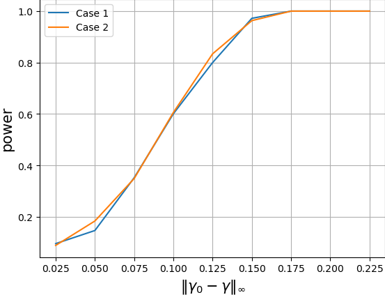
Figure 2 plots the power curve of the hypothesis test of γ=γ0\gamma=\gamma_{0} versus γ≠γ0\gamma\neq\gamma_{0}; here, we use γ0=γ+δ×(1,1,…,1)T\gamma_{0}=\gamma+\delta\times(1,1,...,1)^{T} and δ>0\delta>0.

Refer to caption
Figure 2: Power of the test for cases 1 and 2; the x-axis represents maxi=1,…,p1⁡|γ0,i−γi|\max_{i=1,...,p_{1}}|\gamma_{0,i}-\gamma_{i}|. Nominal size for the test is 5%5\%; see algorithm 25 for the meaning of notations.

7 Conclusion

The paper at hand proposes an improved, i.e., debiased and thresholded, ridge regression method that recovers the sparsity of parameters and avoids introducing a large bias. Besides, it derives a consistency result and the Gaussian approximation theorem for the improved ridge estimator. An asymptotically valid confidence region for γ=M​β\gamma=M\beta and a hypothesis test of γ=γ0\gamma=\gamma_{0} are also constructed based on a wild bootstrap algorithm. In addition, a novel, hybrid resampling procedure was proposed that can be used to perform interval prediction based on the improved ridge regression.

Numerical simulations indicate that improved ridge regression has comparable performance to the threshold Lasso while having at least two major advantages: (a) Ridge regression is easily computed using a closed-form expression, and (b) it appears to be quite robust against a non-optimal choice of the ridge parameter ρn\rho_{n}. Therefore, ridge regression may be found useful again in applied work using high-dimensional data as long as practitioners make sure to include debiasing and thresholding.

References

  • [1] Robert Tibshirani. Regression shrinkage and selection via the lasso. Journal of the Royal Statistical Society: Series B (Methodological), 58(1):267–288, 1996.
  • [2] Nicolai Meinshausen and Peter Bühlmann. High-dimensional graphs and variable selection with the lasso. Ann. Statist., 34(3):1436–1462, 06 2006.
  • [3] Nicolai Meinshausen and Bin Yu. Lasso-type recovery of sparse representations for high-dimensional data. Ann. Statist., 37(1):246–270, 02 2009.
  • [4] Sara A. van de Geer. High-dimensional generalized linear models and the lasso. Ann. Statist., 36(2):614–645, 04 2008.
  • [5] A. Chatterjee and S. N. Lahiri. Asymptotic properties of the residual bootstrap for lasso estimators. Proceedings of the American Mathematical Society, 138(12):4497–4509, 2010.
  • [6] A. Chatterjee and S. N. Lahiri. Bootstrapping lasso estimators. Journal of the American Statistical Association, 106(494):608–625, 2011.
  • [7] Xianyang Zhang and Guang Cheng. Simultaneous inference for high-dimensional linear models. Journal of the American Statistical Association, 112(518):757–768, 2017.
  • [8] Ruben Dezeure, Peter Bühlmann, and Cun-Hui Zhang. High-dimensional simultaneous inference with the bootstrap. TEST, 26(4):685–719, Dec 2017.
  • [9] Adel Javanmard and Andrea Montanari. Debiasing the lasso: Optimal sample size for gaussian designs. Ann. Statist., 46(6A):2593–2622, 12 2018.
  • [10] Jianqing Fan and Runze Li. Variable selection via nonconcave penalized likelihood and its oracle properties. Journal of the American Statistical Association, 96(456):1348–1360, 2001.
  • [11] Xi Chen and Wen-Xin Zhou. Robust inference via multiplier bootstrap. Ann. Statist., 48(3):1665–1691, 06 2020.
  • [12] Sara van de Geer, Peter Bühlmann, and Shuheng Zhou. The adaptive and the thresholded Lasso for potentially misspecified models (and a lower bound for the Lasso). Electronic Journal of Statistics, 5(none):688 – 749, 2011.
  • [13] Peter Bühlmann and Sara van de Geer. Statistics for High-Dimensional Data: Methods, Theory and Applications. Springer-Verlag Berlin Heidelberg, 1st edition, 2011.
  • [14] Sara van de Geer. On the asymptotic variance of the debiased Lasso. Electronic Journal of Statistics, 13(2):2970 – 3008, 2019.
  • [15] Adel Javanmard and Hamid Javadi. False discovery rate control via debiased lasso. Electronic Journal of Statistics, 13(1):1212 – 1253, 2019.
  • [16] Jason D. Lee, Dennis L. Sun, Yuekai Sun, and Jonathan E. Taylor. Exact post-selection inference, with application to the lasso. Ann. Statist., 44(3):907–927, 06 2016.
  • [17] Hanzhong Liu and Bin Yu. Asymptotic properties of lasso+mls and lasso+ridge in sparse high-dimensional linear regression. Electron. J. Statist., 7:3124–3169, 2013.
  • [18] Ryan J. Tibshirani, Alessandro Rinaldo, Rob Tibshirani, and Larry Wasserman. Uniform asymptotic inference and the bootstrap after model selection. Ann. Statist., 46(3):1255–1287, 06 2018.
  • [19] Jun Shao and Xinwei Deng. Estimation in high-dimensional linear models with deterministic design matrices. Ann. Statist., 40(2):812–831, 04 2012.
  • [20] Linlin Dai, Kani Chen, Zhihua Sun, Zhenqiu Liu, and Gang Li. Broken adaptive ridge regression and its asymptotic properties. Journal of Multivariate Analysis, 168:334 – 351, 2018.
  • [21] Edgar Dobriban and Stefan Wager. High-dimensional asymptotics of prediction: Ridge regression and classification. Ann. Statist., 46(1):247–279, 02 2018.
  • [22] Peter Bühlmann. Statistical significance in high-dimensional linear models. Bernoulli, 19(4):1212–1242, 09 2013.
  • [23] Miles Lopes. A residual bootstrap for high-dimensional regression with near low-rank designs. In Advances in Neural Information Processing Systems 27, pages 3239–3247, 2014.
  • [24] Roger A. Horn and Charles R. Johnson. Matrix Analysis. Cambridge University Press, 2012.
  • [25] C. F. J. Wu. Jackknife, Bootstrap and Other Resampling Methods in Regression Analysis. The Annals of Statistics, 14(4):1261 – 1295, 1986.
  • [26] Regina Y. Liu. Bootstrap Procedures under some Non-I.I.D. Models. The Annals of Statistics, 16(4):1696 – 1708, 1988.
  • [27] Enno Mammen. Bootstrap and Wild Bootstrap for High Dimensional Linear Models. The Annals of Statistics, 21(1):255 – 285, 1993.
  • [28] Victor Chernozhukov, Denis Chetverikov, and Kengo Kato. Gaussian approximations and multiplier bootstrap for maxima of sums of high-dimensional random vectors. Ann. Statist., 41(6):2786–2819, 12 2013.
  • [29] Juan J. Dolado and Helmut Lütkepohl. Making wald tests work for cointegrated var systems. Econometric Reviews, 15(4):369–386, 1996.
  • [30] Yixiao Sun. Robust trend inference with series variance estimator and testing-optimal smoothing parameter. Journal of Econometrics, 164(2):345 – 366, 2011.
  • [31] Sílvia Gonçalves and Timothy J. Vogelsang. Block bootstrap hac robust tests: the sophistication of the naive bootstrap. Econometric Theory, 27(4):745 – 791, 2011.
  • [32] Robert A. Stine. Bootstrap prediction intervals for regression. Journal of the American Statistical Association, 80(392):1026–1031, 1985.
  • [33] Dimitris N. Politis. Model-Free Prediction and Regression. Springer-Verlag New York, 2015.
  • [34] Yaniv Romano, Evan Patterson, and Emmanuel Candès. Conformalized quantile regression. In Advances in Neural Information Processing Systems, volume 32, pages 3543–3553. Curran Associates, Inc., 2019.
  • [35] Yaniv Romano, Matteo Sesia, and Emmanuel Candès. Deep knockoffs. Journal of the American Statistical Association, 115(532):1861–1872, 2020.
  • [36] Jun Shao. Mathematical Statistics. Springer-Verlag New York, 2003.
  • [37] Danna Zhang and Wei Biao Wu. Gaussian approximation for high dimensional time series. Ann. Statist., 45(5):1895–1919, 10 2017.
  • [38] Dimitris N. Politis, Joseph P. Romano, and Michael Wolf. Subsampling. Springer-Verlag New York, 1999.
  • [39] Jing Lei and Larry Wasserman. Distribution-free prediction bands for non-parametric regression. Journal of the Royal Statistical Society. Series B (Statistical Methodology), 76(1):71–96, 2014.
  • [40] Victor Chernozhukov, Kaspar Wüthrich, and Yinchu Zhu. Distributional conformal prediction, 2019.
  • [41] Yunyi Zhang and Dimitris N. Politis. Bootstrap prediction intervals with asymptotic conditional validity and unconditional guarantees. (arXiv:2005.09145), 2021.
  • [42] Enno Mammen. Empirical process of residuals for high-dimensional linear models. Ann. Statist., 24(1):307 – 335, 1996.
  • [43] Peter Whittle. Bounds for the moments of linear and quadratic forms in independent variables. Theory of Probability & Its Applications, 5(3):302–305, 1960.
  • [44] Victor Chernozhukov, Denis Chetverikov, and Kengo Kato. Comparison and anti-concentration bounds for maxima of gaussian random vectors. Probability Theory and Related Fields, 162:47–70, 2015.
  • [45] Mengyu Xu, Danna Zhang, and Wei Biao Wu. Pearson’s chi-squared statistics: approximation theory and beyond. Biometrika, 106(3):716–723, 04 2019.

Appendix A Some important lemmas

This section introduces three useful lemmas. Lemma 37 comes from Whittle [43], which directly contributes to the model selection consistency. Lemma 3 and 50 are similar to Chernozhukov et al. [28], they used a joint normal distribution to approximate the distribution of linear combinations of independent random variables.

Lemma 2

Suppose random variables ϵ1,…,ϵn\epsilon_{1},...,\epsilon_{n} are i.i.d., 𝐄​ϵ1=0\mathbf{E}\epsilon_{1}=0, and ∃\exists a constant m>0m>0 such that 𝐄​|ϵ1|m<∞\mathbf{E}|\epsilon_{1}|^{m}<\infty. In addition suppose the matrix Γ=(γi​j)i=1,2,…,k,j=1,2,…,n\Gamma=(\gamma_{ij})_{i=1,2,...,k,j=1,2,...,n} satisfies

max⁡∑j=1ni=1,2,…,k⁡γi​j2≤D,D>0\max_{i=1,2,...,k}\sum_{j=1}^{n}\gamma_{ij}^{2}\leq D,\ D>0 (36)

Then ∃\exists a constant EE which only depends on mm and 𝐄​|ϵ1|m\mathbf{E}|\epsilon_{1}|^{m} such that for ∀δ>0\forall\delta>0,

P​r​o​b​(maxi=1,2,…,k⁡|∑j=1nγi​j​ϵj|>δ)≤k​E​Dm/2δmProb\left(\max_{i=1,2,...,k}|\sum_{j=1}^{n}\gamma_{ij}\epsilon_{j}|>\delta\right)\leq\frac{kED^{m/2}}{\delta^{m}} (37)
Proof.

From theorem 2 in [43], for any i=1,2,…,ki=1,2,...,k,

P​r​o​b​(|∑j=1nγi​j​ϵj|>δ)≤𝐄​|∑j=1nγi​j​ϵj|mδm≤2m​C​(m)​𝐄​|ϵ1|m​(∑j=1nγi​j2)m/2δm≤2m​C​(m)​𝐄​|ϵ1|m​Dm/2δmProb\left(|\sum_{j=1}^{n}\gamma_{ij}\epsilon_{j}|>\delta\right)\leq\frac{\mathbf{E}|\sum_{j=1}^{n}\gamma_{ij}\epsilon_{j}|^{m}}{\delta^{m}}\leq\frac{2^{m}C(m)\mathbf{E}|\epsilon_{1}|^{m}(\sum_{j=1}^{n}\gamma_{ij}^{2})^{m/2}}{\delta^{m}}\leq\frac{2^{m}C(m)\mathbf{E}|\epsilon_{1}|^{m}D^{m/2}}{\delta^{m}} (38)

Choose E=2m​C​(m)​𝐄​|ϵ1|mE=2^{m}C(m)\mathbf{E}|\epsilon_{1}|^{m},

P​r​o​b​(maxi=1,2,…,k⁡|∑j=1nγi​j​ϵj|>δ)≤∑i=1kP​r​o​b​(|∑j=1nγi​j​ϵj|>δ)≤k​E​Dm/2δmProb\left(\max_{i=1,2,...,k}|\sum_{j=1}^{n}\gamma_{ij}\epsilon_{j}|>\delta\right)\leq\sum_{i=1}^{k}Prob\left(|\sum_{j=1}^{n}\gamma_{ij}\epsilon_{j}|>\delta\right)\leq\frac{kED^{m/2}}{\delta^{m}} (39)

∎

Lemma 3

Suppose ϵ=(ϵ1,…,ϵn)T\epsilon=(\epsilon_{1},...,\epsilon_{n})^{T} are joint normal random variables with mean 𝐄​ϵ=0\mathbf{E}\epsilon=0, non-singular covariance matrix 𝐄​ϵ​ϵT\mathbf{E}\epsilon\epsilon^{T}, and positive marginal variance σi2=𝐄​ϵi2>0\sigma_{i}^{2}=\mathbf{E}\epsilon_{i}^{2}>0, i=1,2,…,ni=1,2,...,n. In addition, suppose ∃\exists two constants 0<c0≤C0<∞0<c_{0}\leq C_{0}<\infty such that c0≤σi≤C0c_{0}\leq\sigma_{i}\leq C_{0} for i=1,2,…,ni=1,2,...,n. Then for any given δ>0\delta>0,

supx∈𝐑(P​r​o​b​(maxi=1,2,…,n⁡|ϵi|≤x+δ)−P​r​o​b​(maxi=1,2,…,n⁡|ϵi|≤x))≤C​δ​(log⁡(n)+|log⁡(δ)|+1)\sup_{x\in\mathbf{R}}\left(Prob(\max_{i=1,2,...,n}|\epsilon_{i}|\leq x+\delta)-Prob(\max_{i=1,2,...,n}|\epsilon_{i}|\leq x)\right)\leq C\delta(\sqrt{\log(n)}+\sqrt{|\log(\delta)|}+1) (40)

CC only depends on c0c_{0} and C0C_{0}.

Proof of lemma 3.

First for any i=1,2,…,ni=1,2,...,n,

|ϵi|=max⁡(ϵi,−ϵi)⇒maxi=1,…,n|ϵi|=max⁡(maxi=1,…,n⁡ϵi,maxi=1,…,n−ϵi)\displaystyle|\epsilon_{i}|=\max(\epsilon_{i},-\epsilon_{i})\Rightarrow\max_{i=1,...,n}|\epsilon_{i}|=\max(\max_{i=1,...,n}\epsilon_{i},\max_{i=1,...,n}-\epsilon_{i}) (41)

Therefore, for any x∈𝐑x\in\mathbf{R},

P​r​o​b​(maxi=1,2,…,n⁡|ϵi|≤x+δ)−P​r​o​b​(maxi=1,2,…,n⁡|ϵi|≤x)=P​r​o​b​(0<max⁡(maxi=1,…,n⁡ϵi,maxi=1,…,n−ϵi)−x≤δ)\displaystyle Prob(\max_{i=1,2,...,n}|\epsilon_{i}|\leq x+\delta)-Prob(\max_{i=1,2,...,n}|\epsilon_{i}|\leq x)=Prob(0<\max(\max_{i=1,...,n}\epsilon_{i},\max_{i=1,...,n}-\epsilon_{i})-x\leq\delta) (42)
≤P​r​o​b​(0<maxi=1,…,n⁡ϵi−x≤δ)+P​r​o​b​(0<maxi=1,…,n−ϵi−x≤δ)\displaystyle\leq Prob(0<\max_{i=1,...,n}\epsilon_{i}-x\leq\delta)+Prob(0<\max_{i=1,...,n}-\epsilon_{i}-x\leq\delta)
≤P​r​o​b​(|maxi=1,…,n⁡ϵi−x|≤δ)+P​r​o​b​(|maxi=1,…,n−ϵi−x|≤δ)\displaystyle\leq Prob(|\max_{i=1,...,n}\epsilon_{i}-x|\leq\delta)+Prob(|\max_{i=1,...,n}-\epsilon_{i}-x|\leq\delta)

−ϵ-\epsilon is also joint normal with mean 00 and marginal variance 𝐄​(−ϵj)2=σj2\mathbf{E}(-\epsilon_{j})^{2}=\sigma_{j}^{2}. From theorem 3 and (18), (19) in [44], by defining σ¯=mini=1,2,…,n⁡σi≤maxi=1,2,…,n⁡σi=σ¯\underline{\sigma}=\min_{i=1,2,...,n}\sigma_{i}\leq\max_{i=1,2,...,n}\sigma_{i}=\overline{\sigma}, we have

supx∈𝐑P​r​o​b​(|maxi=1,2,…,n⁡ϵi−x|≤δ)≤2​δσ¯​(log⁡(n)+max⁡(1,log⁡(σ¯)−log⁡(δ)))\displaystyle\sup_{x\in\mathbf{R}}Prob\left(|\max_{i=1,2,...,n}\epsilon_{i}-x|\leq\delta\right)\leq\frac{\sqrt{2}\delta}{\underline{\sigma}}\left(\sqrt{\log(n)}+\sqrt{\max(1,\log(\underline{\sigma})-\log(\delta))}\right) (43)
+4​2​δσ¯×(σ¯σ¯log⁡(n)+2+σ¯σ¯max⁡(0,log⁡(σ¯)−log⁡(δ)))\displaystyle+\frac{4\sqrt{2}\delta}{\underline{\sigma}}\times\left(\frac{\overline{\sigma}}{\underline{\sigma}}\sqrt{\log(n)}+2+\frac{\overline{\sigma}}{\underline{\sigma}}\sqrt{\max(0,\log(\underline{\sigma})-\log(\delta))}\right)
≤2​δc0​(log⁡(n)+1+|log⁡(c0)|+|log⁡(C0)|+|log⁡(δ)|)\displaystyle\leq\frac{\sqrt{2}\delta}{c_{0}}\left(\sqrt{\log(n)}+\sqrt{1+|\log(c_{0})|+|\log(C_{0})|}+\sqrt{|\log(\delta)|}\right)
+4​2​δ​C0c02​(log⁡(n)+2+|log⁡(c0)|+|log⁡(C0)|+|log⁡(δ)|)\displaystyle+\frac{4\sqrt{2}\delta C_{0}}{c_{0}^{2}}\left(\sqrt{\log(n)}+2+\sqrt{|\log(c_{0})|+|\log(C_{0})|}+\sqrt{|\log(\delta)|}\right)
≤(2×(1+|log⁡(c0)|+|log⁡(C0)|)c0+4​2​C0c02​(2+|log⁡(c0)|+|log⁡(C0)|))×δ⁡(log⁡(n)+1+|log⁡(δ)|)\displaystyle\leq\left(\frac{\sqrt{2\times(1+|\log(c_{0})|+|\log(C_{0})|)}}{c_{0}}+\frac{4\sqrt{2}C_{0}}{c_{0}^{2}}(2+\sqrt{|\log(c_{0})|+|\log(C_{0})|})\right)\times\delta\left(\sqrt{\log(n)}+1+\sqrt{|\log(\delta)|}\right)

Choose C=2×(1+|log⁡(c0)|+|log⁡(C0)|)c0+4​2​C0c02​(2+|log⁡(c0)|+|log⁡(C0)|)C=\frac{\sqrt{2\times(1+|\log(c_{0})|+|\log(C_{0})|)}}{c_{0}}+\frac{4\sqrt{2}C_{0}}{c_{0}^{2}}(2+\sqrt{|\log(c_{0})|+|\log(C_{0})|}), which only depends on c0,C0c_{0},\ C_{0}. Then

supx∈𝐑(P​r​o​b​(maxi=1,2,…,n⁡|ϵi|≤x+δ)−P​r​o​b​(maxi=1,2,…,n⁡|ϵi|≤x))≤2​C​δ​(1+log⁡(n)+|log⁡(δ)|)\sup_{x\in\mathbf{R}}(Prob(\max_{i=1,2,...,n}|\epsilon_{i}|\leq x+\delta)-Prob(\max_{i=1,2,...,n}|\epsilon_{i}|\leq x))\leq 2C\delta(1+\sqrt{\log(n)}+\sqrt{|\log(\delta)|}) (44)

∎

Lemma 4

Suppose ϵ=(ϵ1,…​ϵn)T\epsilon=(\epsilon_{1},...\epsilon_{n})^{T} are i.i.d. random variables with 𝐄​ϵ1=0\mathbf{E}\epsilon_{1}=0, 𝐄​ϵ12=σ2\mathbf{E}\epsilon_{1}^{2}=\sigma^{2} and 𝐄​|ϵ1|3<∞\mathbf{E}|\epsilon_{1}|^{3}<\infty. Γ=(γi​j)i=1,2,…,n,j=1,2,…,k\Gamma=(\gamma_{ij})_{i=1,2,...,n,j=1,2,...,k} is an n×kn\times k (1≤k≤n1\leq k\leq n) rank kk matrix. And ∃\exists constants 0<cΓ≤CΓ<∞0<c_{\Gamma}\leq C_{\Gamma}<\infty such that cΓ2≤∑j=1nγj​i2≤CΓ2c_{\Gamma}^{2}\leq\sum_{j=1}^{n}\gamma_{ji}^{2}\leq C_{\Gamma}^{2} for i=1,2,…,ki=1,2,...,k. σ^2=σ^2​(ϵ)\widehat{\sigma}^{2}=\widehat{\sigma}^{2}(\epsilon) is an estimator of σ2\sigma^{2} and random variables ϵ∗|ϵ=(ϵ1∗,…,ϵn∗)T|ϵ\epsilon^{*}|\epsilon=(\epsilon_{1}^{*},...,\epsilon_{n}^{*})^{T}|\epsilon are i.i.d. with ϵ1∗\epsilon^{*}_{1} having normal distribution 𝒩⁡(0,σ^2)\mathcal{N}(0,\widehat{\sigma}^{2}). ϵi∗σ^\frac{\epsilon_{i}^{*}}{\widehat{\sigma}} is independent of ϵ\epsilon for i=1,2,…,ni=1,2,...,n. In addition, suppose one of the following conditions:

C1. ∃\exists a constant 0<ασ≤1/20<\alpha_{\sigma}\leq 1/2 such that

|σ2−σ^2|=Op(n−ασ)and maxj=1,2,…,n,i=1,2,…,k|γj​i|=o(min(n(ασ−1)/2×log−3/2(n),n−1/3×log−3/2(n))|\sigma^{2}-\widehat{\sigma}^{2}|=O_{p}(n^{-\alpha_{\sigma}})\ \ \text{and }\max_{j=1,2,...,n,\ i=1,2,...,k}|\gamma_{ji}|=o(\min(n^{(\alpha_{\sigma}-1)/2}\times\log^{-3/2}(n),\ n^{-1/3}\times\log^{-3/2}(n)) (45)

C2. ∃\exists a constant 0<ασ<1/20<\alpha_{\sigma}<1/2 such that

|σ2−σ^2|=Op(n−ασ),k=o(nασ×log−3(n)),maxj=1,…,n,i=1,…,k|γj​i|=O(n−ασ×log−3/2(n))|\sigma^{2}-\widehat{\sigma}^{2}|=O_{p}(n^{-\alpha_{\sigma}}),\ k=o(n^{\alpha_{\sigma}}\times\log^{-3}(n)),\ \max_{j=1,...,n,i=1,...,k}|\gamma_{ji}|=O(n^{-\alpha_{\sigma}}\times\log^{-3/2}(n)) (46)

Then we have

supx∈[0,∞)|P​r​o​b​(maxi=1,2,…,k⁡|∑j=1nγj​i​ϵj|≤x)−P​r​o​b∗​(maxi=1,2,…,k⁡|∑j=1nγj​i​ϵj∗|≤x)|=oP​(1)\sup_{x\in[0,\infty)}|Prob(\max_{i=1,2,...,k}|\sum_{j=1}^{n}\gamma_{ji}\epsilon_{j}|\leq x)-Prob^{*}(\max_{i=1,2,...,k}|\sum_{j=1}^{n}\gamma_{ji}\epsilon_{j}^{*}|\leq x)|=o_{P}(1) (47)

In particular, if σ^=σ\widehat{\sigma}=\sigma, by assuming one of the following conditions,

C1′.C_{1}^{{}^{\prime}}.

maxj=1,2,…,n,i=1,2,…,k|γj​i|=o(n−1/3×log−3/2(n))\max_{j=1,2,...,n,i=1,2,...,k}|\gamma_{ji}|=o(n^{-1/3}\times\log^{-3/2}(n)) (48)

C2′.C_{2}^{{}^{\prime}}.

k×maxj=1,2,…,n,i=1,2,…,k|γj​i|=o(log−9/2(n))k\times\max_{j=1,2,...,n,i=1,2,...,k}|\gamma_{ji}|=o(\log^{-9/2}(n)) (49)

Then we have

supx∈[0,∞)|P​r​o​b​(maxi=1,2,…,k⁡|∑j=1nγj​i​ϵj|≤x)−P​r​o​b​(maxi=1,2,…,k⁡|∑j=1nγj​i​ϵj∗|≤x)|=o⁡(1)\sup_{x\in[0,\infty)}|Prob(\max_{i=1,2,...,k}|\sum_{j=1}^{n}\gamma_{ji}\epsilon_{j}|\leq x)-Prob(\max_{i=1,2,...,k}|\sum_{j=1}^{n}\gamma_{ji}\epsilon_{j}^{*}|\leq x)|=o(1) (50)
Proof of lemma 50.

In this proof we define Γ=(γ1,…,γk)\Gamma=(\gamma_{1},...,\gamma_{k}) with γi=(γ1​i,γ2​i,…,γn​i)T∈𝐑n\gamma_{i}=(\gamma_{1i},\gamma_{2i},...,\gamma_{ni})^{T}\in\mathbf{R}^{n}. For i=1,2,…,ki=1,2,...,k, γiT​ϵ=∑j=1nγj​i​ϵj\gamma_{i}^{T}\epsilon=\sum_{j=1}^{n}\gamma_{ji}\epsilon_{j}. From lemma A.2 and (8) in [28], and (S1) to (S5) in [45], for x=(x1,…,xn)x=(x_{1},...,x_{n}) and y,z∈𝐑y,z\in\mathbf{R}, define

Fβ​(x)=1β​log⁡(∑i=1nexp⁡(β​xi)),g0​(y)=(1−min⁡(1,max⁡(y,0))4)4,gψ,z​(y)=g0​(ψ⁡(y−z))F_{\beta}(x)=\frac{1}{\beta}\log\left(\sum_{i=1}^{n}\exp(\beta x_{i})\right),\ g_{0}(y)=(1-\min(1,\max(y,0))^{4})^{4},\ g_{\psi,z}(y)=g_{0}(\psi(y-z)) (51)

Here β,ψ>0\beta,\psi>0. Then gψ,z∈𝐂3g_{\psi,z}\in\mathbf{C}^{3} is nonincreasing function. g0=1g_{0}=1 with y≤0y\leq 0, 00 with y≥1y\geq 1, and

g∗=maxy∈𝐑(|g0′(y)|+|g0′′(y)|+|g0′′′(y)|)<∞, 1y≤z≤gψ,z(y)≤𝟏y≤z+ψ−1\displaystyle g_{*}=\max_{y\in\mathbf{R}}(|g_{0}^{{}^{\prime}}(y)|+|g_{0}^{{}^{\prime\prime}}(y)|+|g_{0}^{{}^{\prime\prime\prime}}(y)|)<\infty,\ \mathbf{1}_{y\leq z}\leq g_{\psi,z}(y)\leq\mathbf{1}_{y\leq z+\psi^{-1}} (52)
supy,z∈𝐑|gψ,z′(y)|≤g∗ψ,supy,z∈𝐑|gψ,z′′(y)|≤g∗ψ2,supy,z∈𝐑|gψ,z′′′(y)|≤g∗ψ3\displaystyle\sup_{y,z\in\mathbf{R}}|g_{\psi,z}^{{}^{\prime}}(y)|\leq g_{*}\psi,\ \sup_{y,z\in\mathbf{R}}|g_{\psi,z}^{{}^{\prime\prime}}(y)|\leq g_{*}\psi^{2},\ \sup_{y,z\in\mathbf{R}}|g_{\psi,z}^{{}^{\prime\prime\prime}}(y)|\leq g_{*}\psi^{3}
∂Fβ∂xi=exp⁡(β​xi)∑j=1nexp⁡(β​xj)⇒∂Fβ∂xi≥0,∑i=1n∂Fβ∂xi=1,∑i=1n∑j=1n|∂2Fβ∂xi​∂xj|≤2​β,∑i=1n∑j=1n∑k=1n|∂3Fβ∂xi​∂xj​∂xk|≤6​β2\displaystyle\frac{\partial F_{\beta}}{\partial x_{i}}=\frac{\exp(\beta x_{i})}{\sum_{j=1}^{n}\exp(\beta x_{j})}\Rightarrow\frac{\partial F_{\beta}}{\partial x_{i}}\geq 0,\ \sum_{i=1}^{n}\frac{\partial F_{\beta}}{\partial x_{i}}=1,\ \sum_{i=1}^{n}\sum_{j=1}^{n}|\frac{\partial^{2}F_{\beta}}{\partial x_{i}\partial x_{j}}|\leq 2\beta,\ \sum_{i=1}^{n}\sum_{j=1}^{n}\sum_{k=1}^{n}|\frac{\partial^{3}F_{\beta}}{\partial x_{i}\partial x_{j}\partial x_{k}}|\leq 6\beta^{2}
Fβ​(x1,…,xn)−log⁡(n)β≤maxi=1,…,n⁡xi≤Fβ​(x1,…,xn)\displaystyle F_{\beta}(x_{1},...,x_{n})-\frac{\log(n)}{\beta}\leq\max_{i=1,...,n}x_{i}\leq F_{\beta}(x_{1},...,x_{n})

For any given x=(x1,…,xn)∈𝐑nx=(x_{1},...,x_{n})\in\mathbf{R}^{n}, define function

Gβ​(x)=1β​log⁡(∑i=1nexp⁡(β​xi)+∑i=1nexp⁡(−β​xi))=Fβ​(x1,…,xn,−x1,…,−xn)G_{\beta}(x)=\frac{1}{\beta}\log(\sum_{i=1}^{n}\exp(\beta x_{i})+\sum_{i=1}^{n}\exp(-\beta x_{i}))=F_{\beta}(x_{1},...,x_{n},-x_{1},...,-x_{n}). From (52) and (41), for i,j,k=1,…,ni,j,k=1,...,n

Gβ​(x)−log⁡(2​n)β≤maxi=1,…,n⁡|xi|≤Gβ​(x),∂Gβ∂xi=∂Fβ∂xi−∂Fβ∂xi+n⇒∑i=1n|∂Gβ∂xi|≤∑i=1n∂Fβ∂xi+∂Fβ∂xi+n=1\displaystyle G_{\beta}(x)-\frac{\log(2n)}{\beta}\leq\max_{i=1,...,n}|x_{i}|\leq G_{\beta}(x),\ \frac{\partial G_{\beta}}{\partial x_{i}}=\frac{\partial F_{\beta}}{\partial x_{i}}-\frac{\partial F_{\beta}}{\partial x_{i+n}}\Rightarrow\sum_{i=1}^{n}|\frac{\partial G_{\beta}}{\partial x_{i}}|\leq\sum_{i=1}^{n}\frac{\partial F_{\beta}}{\partial x_{i}}+\frac{\partial F_{\beta}}{\partial x_{i+n}}=1 (53)
∂2Gβ∂xi​∂xj=∂2Fβ∂xi​∂xj−∂2Fβ∂xi​∂xj+n−∂2Fβ∂xi+n​∂xj+∂2Fβ∂xi+n​∂xj+n⇒∑i=1n∑j=1n|∂2Gβ∂xi​∂xj|≤∑i=12​n∑j=12​n|∂2Fβ∂xi​∂xj|≤2​β\displaystyle\frac{\partial^{2}G_{\beta}}{\partial x_{i}\partial x_{j}}=\frac{\partial^{2}F_{\beta}}{\partial x_{i}\partial x_{j}}-\frac{\partial^{2}F_{\beta}}{\partial x_{i}\partial x_{j+n}}-\frac{\partial^{2}F_{\beta}}{\partial x_{i+n}\partial x_{j}}+\frac{\partial^{2}F_{\beta}}{\partial x_{i+n}\partial x_{j+n}}\Rightarrow\sum_{i=1}^{n}\sum_{j=1}^{n}|\frac{\partial^{2}G_{\beta}}{\partial x_{i}\partial x_{j}}|\leq\sum_{i=1}^{2n}\sum_{j=1}^{2n}|\frac{\partial^{2}F_{\beta}}{\partial x_{i}\partial x_{j}}|\leq 2\beta
∂3Gβ∂xi​∂xj​∂xk=∂3Fβ∂xi​∂xj​∂xk−∂3Fβ∂xi​∂xj​∂xk+n−∂3Fβ∂xi​∂xj+n​∂xk+∂3Fβ∂xi​∂xj+n​∂xk+n−∂3Fβ∂xi+n​∂xj​∂xk+∂3Fβ∂xi+n​∂xj​∂xk+n\displaystyle\frac{\partial^{3}G_{\beta}}{\partial x_{i}\partial x_{j}\partial x_{k}}=\frac{\partial^{3}F_{\beta}}{\partial x_{i}\partial x_{j}\partial x_{k}}-\frac{\partial^{3}F_{\beta}}{\partial x_{i}\partial x_{j}\partial x_{k+n}}-\frac{\partial^{3}F_{\beta}}{\partial x_{i}\partial x_{j+n}\partial x_{k}}+\frac{\partial^{3}F_{\beta}}{\partial x_{i}\partial x_{j+n}\partial x_{k+n}}-\frac{\partial^{3}F_{\beta}}{\partial x_{i+n}\partial x_{j}\partial x_{k}}+\frac{\partial^{3}F_{\beta}}{\partial x_{i+n}\partial x_{j}\partial x_{k+n}}
+∂3Fβ∂xi+n​∂xj+n​∂xk−∂3Fβ∂xi+n​∂xj+n​∂xk+n⇒∑i=1n∑j=1n∑k=1n|∂3Gβ∂xi​∂xj​∂xk|≤∑i=12​n∑j=12​n∑k=12​n|∂3Fβ∂xi​∂xj​∂xk|≤6​β2\displaystyle+\frac{\partial^{3}F_{\beta}}{\partial x_{i+n}\partial x_{j+n}\partial x_{k}}-\frac{\partial^{3}F_{\beta}}{\partial x_{i+n}\partial x_{j+n}\partial x_{k+n}}\Rightarrow\sum_{i=1}^{n}\sum_{j=1}^{n}\sum_{k=1}^{n}|\frac{\partial^{3}G_{\beta}}{\partial x_{i}\partial x_{j}\partial x_{k}}|\leq\sum_{i=1}^{2n}\sum_{j=1}^{2n}\sum_{k=1}^{2n}|\frac{\partial^{3}F_{\beta}}{\partial x_{i}\partial x_{j}\partial x_{k}}|\leq 6\beta^{2}

Define hβ,ψ,x​(x1,…,xn)=gψ,x​(Gβ​(x1,…,xn))h_{\beta,\psi,x}(x_{1},...,x_{n})=g_{\psi,x}(G_{\beta}(x_{1},...,x_{n})). Direct calculation shows ∂hβ,ψ,x​(x1,…,xn)∂xi=gψ,x′(Gβ(x1,…,xn))∂Gβ∂xi⇒∑i=1n|∂hβ,ψ,x​(x1,…,xn)∂xi|≤g∗ψ\frac{\partial h_{\beta,\psi,x}(x_{1},...,x_{n})}{\partial x_{i}}=g^{{}^{\prime}}_{\psi,x}(G_{\beta}(x_{1},...,x_{n}))\frac{\partial G_{\beta}}{\partial x_{i}}\Rightarrow\sum_{i=1}^{n}|\frac{\partial h_{\beta,\psi,x}(x_{1},...,x_{n})}{\partial x_{i}}|\leq g_{*}\psi;

∂2hβ,ψ,x​(x1,…,xn)∂xi​∂xj=g′′ψ,x(Gβ(x1,…,xn))∂Gβ∂xi∂Gβ∂xj+g′ψ,x(Gβ(x1,…,xn))∂2Gβ∂xi​∂xj\displaystyle\frac{\partial^{2}h_{\beta,\psi,x}(x_{1},...,x_{n})}{\partial x_{i}\partial x_{j}}=g^{{}^{\prime\prime}}_{\psi,x}(G_{\beta}(x_{1},...,x_{n}))\frac{\partial G_{\beta}}{\partial x_{i}}\frac{\partial G_{\beta}}{\partial x_{j}}+g^{{}^{\prime}}_{\psi,x}(G_{\beta}(x_{1},...,x_{n}))\frac{\partial^{2}G_{\beta}}{\partial x_{i}\partial x_{j}} (54)
⇒∑i=1n∑j=1n|∂2hβ,ψ,x​(x1,…,xn)∂xi​∂xj|≤g∗​ψ2​(∑i=1n|∂Gβ∂xi|)2+g∗​ψ​∑i=1n∑j=1n|∂2Gβ∂xi​∂xj|≤g∗​ψ2+2​g∗​ψ​β\displaystyle\Rightarrow\sum_{i=1}^{n}\sum_{j=1}^{n}|\frac{\partial^{2}h_{\beta,\psi,x}(x_{1},...,x_{n})}{\partial x_{i}\partial x_{j}}|\leq g_{*}\psi^{2}\left(\sum_{i=1}^{n}|\frac{\partial G_{\beta}}{\partial x_{i}}|\right)^{2}+g_{*}\psi\sum_{i=1}^{n}\sum_{j=1}^{n}|\frac{\partial^{2}G_{\beta}}{\partial x_{i}\partial x_{j}}|\leq g_{*}\psi^{2}+2g_{*}\psi\beta
and ∂3hβ,ψ,x​(x1,…,xn)∂xi​∂xj​∂xk=g′′′ψ,x(Gβ(x1,…,xn))∂Gβ∂xi∂Gβ∂xj∂Gβ∂xk+g′′ψ,x(Gβ(x1,…,xn))∂2Gβ∂xi​∂xk∂Gβ∂xj\displaystyle\text{and }\frac{\partial^{3}h_{\beta,\psi,x}(x_{1},...,x_{n})}{\partial x_{i}\partial x_{j}\partial x_{k}}=g^{{}^{\prime\prime\prime}}_{\psi,x}(G_{\beta}(x_{1},...,x_{n}))\frac{\partial G_{\beta}}{\partial x_{i}}\frac{\partial G_{\beta}}{\partial x_{j}}\frac{\partial G_{\beta}}{\partial x_{k}}+g^{{}^{\prime\prime}}_{\psi,x}(G_{\beta}(x_{1},...,x_{n}))\frac{\partial^{2}G_{\beta}}{\partial x_{i}\partial x_{k}}\frac{\partial G_{\beta}}{\partial x_{j}}
+g′′ψ,x(Gβ(x1,…,xn))∂Gβ∂xi∂2Gβ∂xj​∂xk+g′′ψ,x(Gβ(x1,…,xn))∂2Gβ∂xi​∂xj∂Gβ∂xk+g′ψ,x(Gβ(x1,…,xn))∂3Gβ∂xi​∂xj​∂xk\displaystyle+g^{{}^{\prime\prime}}_{\psi,x}(G_{\beta}(x_{1},...,x_{n}))\frac{\partial G_{\beta}}{\partial x_{i}}\frac{\partial^{2}G_{\beta}}{\partial x_{j}\partial x_{k}}+g^{{}^{\prime\prime}}_{\psi,x}(G_{\beta}(x_{1},...,x_{n}))\frac{\partial^{2}G_{\beta}}{\partial x_{i}\partial x_{j}}\frac{\partial G_{\beta}}{\partial x_{k}}+g^{{}^{\prime}}_{\psi,x}(G_{\beta}(x_{1},...,x_{n}))\frac{\partial^{3}G_{\beta}}{\partial x_{i}\partial x_{j}\partial x_{k}}
⇒∑i=1n∑j=1n∑k=1n|∂3hβ,ψ,x​(x1,…,xn)∂xi​∂xj​∂xk|≤g∗​ψ3​(∑i=1n|∂Gβ∂xi|)3+3​g∗​ψ2​(∑i=1n∑j=1n|∂2Gβ∂xi​∂xj|)×(∑k=1n|∂Gβ∂xk|)\displaystyle\Rightarrow\sum_{i=1}^{n}\sum_{j=1}^{n}\sum_{k=1}^{n}|\frac{\partial^{3}h_{\beta,\psi,x}(x_{1},...,x_{n})}{\partial x_{i}\partial x_{j}\partial x_{k}}|\leq g_{*}\psi^{3}\left(\sum_{i=1}^{n}|\frac{\partial G_{\beta}}{\partial x_{i}}|\right)^{3}+3g_{*}\psi^{2}\left(\sum_{i=1}^{n}\sum_{j=1}^{n}|\frac{\partial^{2}G_{\beta}}{\partial x_{i}\partial x_{j}}|\right)\times\left(\sum_{k=1}^{n}|\frac{\partial G_{\beta}}{\partial x_{k}}|\right)
+g∗ψ∑i=1n∑j=1n∑k=1n|∂3Gβ∂xi​∂xj​∂xk|≤g∗ψ3+6g∗ψ2β+6g∗ψβ2\displaystyle+g_{*}\psi\sum_{i=1}^{n}\sum_{j=1}^{n}\sum_{k=1}^{n}|\frac{\partial^{3}G_{\beta}}{\partial x_{i}\partial x_{j}\partial x_{k}}|\leq g_{*}\psi^{3}+6g_{*}\psi^{2}\beta+6g_{*}\psi\beta^{2}

Define ξ=(ξ1,…,ξn)\xi=(\xi_{1},...,\xi_{n}) as i.i.d. random variables with the same marginal distribution as ϵ1\epsilon_{1}, and is independent of ϵ,ϵ∗\epsilon,\epsilon^{*}. Therefore, P​r​o​b​(maxi=1,2,…,k⁡|γiT​ϵ|≤x)=P​r​o​b∗​(maxi=1,2,…,k⁡|∑j=1nγiT​ξ|≤x)Prob(\max_{i=1,2,...,k}|\gamma_{i}^{T}\epsilon|\leq x)=Prob^{*}(\max_{i=1,2,...,k}|\sum_{j=1}^{n}\gamma_{i}^{T}\xi|\leq x) for any xx. Since cΓ2≤𝐄∗​(∑l=1nγi​l​ϵl∗σ^)2=∑l=1nγi​l2≤CΓ2​for i=1,2,…,kc_{\Gamma}^{2}\leq\mathbf{E}^{*}\left(\sum_{l=1}^{n}\frac{\gamma_{il}\epsilon^{*}_{l}}{\widehat{\sigma}}\right)^{2}=\sum_{l=1}^{n}\gamma_{il}^{2}\leq C_{\Gamma}^{2}\ \text{for $i=1,2,...,k$}. According to (41), (53) and lemma 3, ∃\exists a constant CC which only depends on cΓc_{\Gamma} and CΓC_{\Gamma} such that for any given ψ,β,σ^>0\psi,\beta,\widehat{\sigma}>0,

supx∈𝐑(P​r​o​b∗​(maxi=1,2,…,k⁡|γiT​ϵ∗|≤x+1ψ+log⁡(2​k)β)−P​r​o​b∗​(maxi=1,2,…,k⁡|γiT​ϵ∗|≤x))\displaystyle\sup_{x\in\mathbf{R}}\left(Prob^{*}\left(\max_{i=1,2,...,k}|\gamma_{i}^{T}\epsilon^{*}|\leq x+\frac{1}{\psi}+\frac{\log(2k)}{\beta}\right)-Prob^{*}\left(\max_{i=1,2,...,k}|\gamma_{i}^{T}\epsilon^{*}|\leq x\right)\right) (55)
=supx∈𝐑(P​r​o​b∗​(maxi=1,2,…,k⁡|γiT​ϵ∗σ^|≤xσ^+1ψ​σ^+log⁡(2​k)β​σ^)−P​r​o​b∗​(maxi=1,2,…,k⁡|γiT​ϵ∗σ^|≤xσ^))\displaystyle=\sup_{x\in\mathbf{R}}\left(Prob^{*}\left(\max_{i=1,2,...,k}|\frac{\gamma_{i}^{T}\epsilon^{*}}{\widehat{\sigma}}|\leq\frac{x}{\widehat{\sigma}}+\frac{1}{\psi\widehat{\sigma}}+\frac{\log(2k)}{\beta\widehat{\sigma}}\right)-Prob^{*}\left(\max_{i=1,2,...,k}|\frac{\gamma_{i}^{T}\epsilon^{*}}{\widehat{\sigma}}|\leq\frac{x}{\widehat{\sigma}}\right)\right)
≤C×(1ψ​σ^+log⁡(2​k)β​σ^)×(1+log⁡(n)+|log⁡(1ψ​σ^+log⁡(2​k)β​σ^)|)\displaystyle\leq C\times\left(\frac{1}{\psi\widehat{\sigma}}+\frac{\log(2k)}{\beta\widehat{\sigma}}\right)\times\left(1+\sqrt{\log(n)}+\sqrt{|\log\left(\frac{1}{\psi\widehat{\sigma}}+\frac{\log(2k)}{\beta\widehat{\sigma}}\right)|}\right)

Define z=C×(1ψ​σ^+log⁡(2​k)β​σ^)×(1+log⁡(n)+|log⁡(1ψ​σ^+log⁡(2​k)β​σ^)|)z=C\times\left(\frac{1}{\psi\widehat{\sigma}}+\frac{\log(2k)}{\beta\widehat{\sigma}}\right)\times\left(1+\sqrt{\log(n)}+\sqrt{|\log\left(\frac{1}{\psi\widehat{\sigma}}+\frac{\log(2k)}{\beta\widehat{\sigma}}\right)|}\right). For any x≥0x\geq 0,

P​r​o​b​(maxi=1,2,…,k⁡|γiT​ϵ|≤x)−P​r​o​b∗​(maxi=1,2,…,k⁡|γiT​ϵ∗|≤x)\displaystyle Prob(\max_{i=1,2,...,k}|\gamma_{i}^{T}\epsilon|\leq x)-Prob^{*}(\max_{i=1,2,...,k}|\gamma_{i}^{T}\epsilon^{*}|\leq x) (56)
≤P​r​o​b∗​(maxi=1,2,…,k⁡|γiT​ξ|≤x)−P​r​o​b∗​(maxi=1,2,…,k⁡|γiT​ϵ∗|≤x+1ψ+log⁡(2​k)β)+z\displaystyle\leq Prob^{*}(\max_{i=1,2,...,k}|\gamma_{i}^{T}\xi|\leq x)-Prob^{*}(\max_{i=1,2,...,k}|\gamma_{i}^{T}\epsilon^{*}|\leq x+\frac{1}{\psi}+\frac{\log(2k)}{\beta})+z
≤P​r​o​b∗​(Gβ​(γ1T​ξ,…,γkT​ξ)≤x+log⁡(2​k)β)−P​r​o​b∗​(Gβ​(γ1T​ϵ∗,…,γkT​ϵ∗)≤x+1ψ+log⁡(2​k)β)+z\displaystyle\leq Prob^{*}(G_{\beta}(\gamma_{1}^{T}\xi,...,\gamma_{k}^{T}\xi)\leq x+\frac{\log(2k)}{\beta})-Prob^{*}(G_{\beta}(\gamma_{1}^{T}\epsilon^{*},...,\gamma_{k}^{T}\epsilon^{*})\leq x+\frac{1}{\psi}+\frac{\log(2k)}{\beta})+z
≤𝐄∗​hβ,ψ,x+log⁡(2​k)β​(γ1T​ξ,…,γkT​ξ)−hβ,ψ,x+log⁡(2​k)β​(γ1T​ϵ∗,…,γkT​ϵ∗)+z\displaystyle\leq\mathbf{E}^{*}h_{\beta,\psi,x+\frac{\log(2k)}{\beta}}(\gamma_{1}^{T}\xi,...,\gamma_{k}^{T}\xi)-h_{\beta,\psi,x+\frac{\log(2k)}{\beta}}(\gamma_{1}^{T}\epsilon^{*},...,\gamma_{k}^{T}\epsilon^{*})+z
P​r​o​b​(maxi=1,2,…,k⁡|γiT​ϵ|≤x)−P​r​o​b∗​(maxi=1,2,…,k⁡|γiT​ϵ∗|≤x)\displaystyle Prob(\max_{i=1,2,...,k}|\gamma_{i}^{T}\epsilon|\leq x)-Prob^{*}(\max_{i=1,2,...,k}|\gamma_{i}^{T}\epsilon^{*}|\leq x)
≥P​r​o​b∗​(maxi=1,2,…,k⁡|γiT​ξ|≤x)−P​r​o​b∗​(maxi=1,2,…,k⁡|γiT​ϵ∗|≤x−1ψ−log⁡(2​k)β)−z\displaystyle\geq Prob^{*}(\max_{i=1,2,...,k}|\gamma_{i}^{T}\xi|\leq x)-Prob^{*}(\max_{i=1,2,...,k}|\gamma_{i}^{T}\epsilon^{*}|\leq x-\frac{1}{\psi}-\frac{\log(2k)}{\beta})-z
≥P​r​o​b∗​(Gβ​(γ1T​ξ,…,γkT​ξ)≤x)−P​r​o​b∗​(Gβ​(γ1T​ϵ∗,…,γkT​ϵ∗)≤x−1ψ)−z\displaystyle\geq Prob^{*}(G_{\beta}(\gamma_{1}^{T}\xi,...,\gamma_{k}^{T}\xi)\leq x)-Prob^{*}(G_{\beta}(\gamma_{1}^{T}\epsilon^{*},...,\gamma_{k}^{T}\epsilon^{*})\leq x-\frac{1}{\psi})-z
≥𝐄∗​hβ,ψ,x−1ψ​(γ1T​ξ,…,γkT​ξ)−hβ,ψ,x−1ψ​(γ1T​ϵ∗,…,γkT​ϵ∗)−z\displaystyle\geq\mathbf{E}^{*}h_{\beta,\psi,x-\frac{1}{\psi}}(\gamma_{1}^{T}\xi,...,\gamma_{k}^{T}\xi)-h_{\beta,\psi,x-\frac{1}{\psi}}(\gamma_{1}^{T}\epsilon^{*},...,\gamma_{k}^{T}\epsilon^{*})-z

Therefore, we have

supx∈[0,∞)|P​r​o​b​(maxi=1,2,…,k⁡|γiT​ϵ|≤x)−P​r​o​b∗​(maxi=1,2,…,k⁡|γiT​ϵ∗|≤x)|≤z+supx∈𝐑|𝐄∗​hβ,ψ,x​(γ1T​ξ,…,γkT​ξ)−hβ,ψ,x​(γ1T​ϵ∗,…,γkT​ϵ∗)|\displaystyle\sup_{x\in[0,\infty)}|Prob(\max_{i=1,2,...,k}|\gamma_{i}^{T}\epsilon|\leq x)-Prob^{*}(\max_{i=1,2,...,k}|\gamma_{i}^{T}\epsilon^{*}|\leq x)|\leq z+\sup_{x\in\mathbf{R}}|\mathbf{E}^{*}h_{\beta,\psi,x}(\gamma_{1}^{T}\xi,...,\gamma_{k}^{T}\xi)-h_{\beta,\psi,x}(\gamma_{1}^{T}\epsilon^{*},...,\gamma_{k}^{T}\epsilon^{*})| (57)

For any i=1,2,…,k,j=1,2,…,ni=1,2,...,k,j=1,2,...,n, define Hi​j=∑s=1j−1γs​i​ξs+∑s=j+1nγs​i​ϵs∗H_{ij}=\sum_{s=1}^{j-1}\gamma_{si}\xi_{s}+\sum_{s=j+1}^{n}\gamma_{si}\epsilon_{s}^{*}, mi​j=γj​i​ξjm_{ij}=\gamma_{ji}\xi_{j} and mi​j∗=γj​i​ϵj∗m^{*}_{ij}=\gamma_{ji}\epsilon^{*}_{j}, we have Hi​j+mi​j=Hi​j+1+mi​j+1∗H_{ij}+m_{ij}=H_{ij+1}+m^{*}_{ij+1}, and

supx∈𝐑|𝐄∗​hβ,ψ,x​(γ1T​ξ,…,γkT​ξ)−hβ,ψ,x​(γ1T​ϵ∗,…,γkT​ϵ∗)|\displaystyle\sup_{x\in\mathbf{R}}|\mathbf{E}^{*}h_{\beta,\psi,x}(\gamma_{1}^{T}\xi,...,\gamma_{k}^{T}\xi)-h_{\beta,\psi,x}(\gamma_{1}^{T}\epsilon^{*},...,\gamma_{k}^{T}\epsilon^{*})| (58)
=supx∈𝐑|∑s=1n𝐄∗​hβ,ψ,x​(H1​s+m1​s,…,Hk​s+mk​s)−hβ,ψ,x​(H1​s+m1​s∗,…,Hk​s+mk​s∗)|\displaystyle=\sup_{x\in\mathbf{R}}|\sum_{s=1}^{n}\mathbf{E}^{*}h_{\beta,\psi,x}(H_{1s}+m_{1s},...,H_{ks}+m_{ks})-h_{\beta,\psi,x}(H_{1s}+m_{1s}^{*},...,H_{ks}+m_{ks}^{*})|
≤∑s=1nsupx∈𝐑|𝐄∗​hβ,ψ,x​(H1​s+m1​s,…,Hk​s+mk​s)−hβ,ψ,x​(H1​s+m1​s∗,…,Hk​s+mk​s∗)|\displaystyle\leq\sum_{s=1}^{n}\sup_{x\in\mathbf{R}}|\mathbf{E}^{*}h_{\beta,\psi,x}(H_{1s}+m_{1s},...,H_{ks}+m_{ks})-h_{\beta,\psi,x}(H_{1s}+m_{1s}^{*},...,H_{ks}+m_{ks}^{*})|

Since 𝐄⁡(ξs|ϵ,ξb,ϵb∗,b≠s)=𝐄⁡(ϵs∗|ϵ,ξb,ϵb∗,b≠s)=0\mathbf{E}(\xi_{s}|\epsilon,\xi_{b},\epsilon^{*}_{b},b\neq s)=\mathbf{E}(\epsilon^{*}_{s}|\epsilon,\xi_{b},\epsilon^{*}_{b},b\neq s)=0, 𝐄⁡(ξs2−ϵs∗2|ϵ,ξb,ϵb∗,b≠s)=σ2−σ^2\mathbf{E}(\xi_{s}^{2}-\epsilon^{*2}_{s}|\epsilon,\xi_{b},\epsilon^{*}_{b},b\neq s)=\sigma^{2}-\widehat{\sigma}^{2}, from multivariate Taylor’s theorem and (54), for any s=1,2,…,ns=1,2,...,n and x∈𝐑x\in\mathbf{R},

|𝐄(hβ,ψ,x(H1​s+m1​s,…,Hk​s+mk​s)−hβ,ψ,x(H1​s+m1​s∗,…,Hk​s+mk​s∗))|ϵ,ξb,ϵ∗b,b≠s|\displaystyle|\mathbf{E}\left(h_{\beta,\psi,x}(H_{1s}+m_{1s},...,H_{ks}+m_{ks})-h_{\beta,\psi,x}(H_{1s}+m_{1s}^{*},...,H_{ks}+m_{ks}^{*})\right)\Big|\epsilon,\xi_{b},\epsilon^{*}_{b},b\neq s| (59)
≤|∑i=1k∂hβ,ψ,x​(H1​s,…,Hk​s)∂xi​γs​i​𝐄​(ξs−ϵs∗|ϵ,ξb,ϵb∗,b≠s)|+12​|∑i=1k∑j=1k∂2hβ,ψ,x​(H1​s,…,Hk​s)∂xi​∂xj​γs​i​γs​j​𝐄​(ξs2−ϵs∗2|ϵ,ξb,ϵb∗,b≠s)|\displaystyle\leq|\sum_{i=1}^{k}\frac{\partial h_{\beta,\psi,x}(H_{1s},...,H_{ks})}{\partial x_{i}}\gamma_{si}\mathbf{E}(\xi_{s}-\epsilon^{*}_{s}|\epsilon,\xi_{b},\epsilon^{*}_{b},b\neq s)|+\frac{1}{2}|\sum_{i=1}^{k}\sum_{j=1}^{k}\frac{\partial^{2}h_{\beta,\psi,x}(H_{1s},...,H_{ks})}{\partial x_{i}\partial x_{j}}\gamma_{si}\gamma_{sj}\mathbf{E}(\xi_{s}^{2}-\epsilon^{*2}_{s}|\epsilon,\xi_{b},\epsilon^{*}_{b},b\neq s)|
+(g∗ψ3+g∗ψ2β+g∗ψβ2)maxi=1,2,…,k|γs​i|3×(𝐄|ϵ1|3+σ^3D)\displaystyle+(g_{*}\psi^{3}+g_{*}\psi^{2}\beta+g_{*}\psi\beta^{2})\max_{i=1,2,...,k}|\gamma_{si}|^{3}\times(\mathbf{E}|\epsilon_{1}|^{3}+\widehat{\sigma}^{3}D)
⇒supx∈𝐑|𝐄hβ,ψ,x(H1​s+m1​s,…,Hk​s+mk​s)−hβ,ψ,x(H1​s+m1​s∗,…,Hk​s+mk​s∗)|ϵ,ξb,ϵ∗b,b≠s|\displaystyle\Rightarrow\sup_{x\in\mathbf{R}}|\mathbf{E}h_{\beta,\psi,x}(H_{1s}+m_{1s},...,H_{ks}+m_{ks})-h_{\beta,\psi,x}(H_{1s}+m_{1s}^{*},...,H_{ks}+m_{ks}^{*})|\epsilon,\xi_{b},\epsilon^{*}_{b},b\neq s|
≤g∗​(ψ2+ψ​β)​|σ2−σ^2|×maxi=1,…,k⁡γs​i2+(𝐄​|ϵ1|3+σ^3​D)×g∗​(ψ3+ψ2​β+ψ​β2)×maxi=1,…,k⁡|γs​i|3\displaystyle\leq g_{*}(\psi^{2}+\psi\beta)|\sigma^{2}-\widehat{\sigma}^{2}|\times\max_{i=1,...,k}\gamma_{si}^{2}+(\mathbf{E}|\epsilon_{1}|^{3}+\widehat{\sigma}^{3}D)\times g_{*}(\psi^{3}+\psi^{2}\beta+\psi\beta^{2})\times\max_{i=1,...,k}|\gamma_{si}|^{3}

Here D=𝐄​|Y|3D=\mathbf{E}|Y|^{3} with YY having normal distribution with mean 00 and variance 11. Then

supx∈[0,∞)|P​r​o​b​(maxi=1,2,…,k⁡|γiT​ϵ|≤x)−P​r​o​b∗​(maxi=1,2,…,k⁡|γiT​ϵ∗|≤x)|\displaystyle\sup_{x\in[0,\infty)}|Prob(\max_{i=1,2,...,k}|\gamma_{i}^{T}\epsilon|\leq x)-Prob^{*}(\max_{i=1,2,...,k}|\gamma_{i}^{T}\epsilon^{*}|\leq x)| (60)
≤z+(g∗​ψ2+g∗​ψ​β)​|σ2−σ^2|×∑s=1nmaxi=1,…,k⁡γs​i2+(𝐄​|ϵ1|3+σ^3​D)×g∗​(ψ3+ψ2​β+ψ​β2)×∑s=1nmaxi=1,…,k⁡|γs​i|3\displaystyle\leq z+(g_{*}\psi^{2}+g_{*}\psi\beta)|\sigma^{2}-\widehat{\sigma}^{2}|\times\sum_{s=1}^{n}\max_{i=1,...,k}\gamma_{si}^{2}+(\mathbf{E}|\epsilon_{1}|^{3}+\widehat{\sigma}^{3}D)\times g_{*}(\psi^{3}+\psi^{2}\beta+\psi\beta^{2})\times\sum_{s=1}^{n}\max_{i=1,...,k}|\gamma_{si}|^{3}

In particular, for any given δ>0\delta>0, choose ψ=β=log3/2⁡(n)/δ1/4\psi=\beta=\log^{3/2}(n)/\delta^{1/4} and suppose 3​σ2>σ^>σ2\frac{3\sigma}{2}>\widehat{\sigma}>\frac{\sigma}{2}. For sufficiently large nn we have 1ψ​σ^+log⁡(2​k)β​σ^≤4​log⁡(n)ψ​σ≤4​δ1/4σ​log⁡(n)<1\frac{1}{\psi\widehat{\sigma}}+\frac{\log(2k)}{\beta\widehat{\sigma}}\leq\frac{4\log(n)}{\psi\sigma}\leq\frac{4\delta^{1/4}}{\sigma\sqrt{\log(n)}}<1 and

z≤4​C​log⁡(n)ψ​σ×(2log⁡(n)+log⁡(ψ​σ^))≤4​C​δ1/4σ(2+32​log⁡(log⁡(n))+log⁡(3​σ/2​δ1/4)log⁡(n))≤C′δ1/4,C′=12​Cσz\leq\frac{4C\log(n)}{\psi\sigma}\times\left(2\sqrt{\log(n)}+\sqrt{\log(\psi\widehat{\sigma})}\right)\leq\frac{4C\delta^{1/4}}{\sigma}\left(2+\sqrt{\frac{\frac{3}{2}\log(\log(n))+\log(3\sigma/2\delta^{1/4})}{\log(n)}}\right)\leq C^{{}^{\prime}}\delta^{1/4},\ C^{{}^{\prime}}=\frac{12C}{\sigma} (61)

Suppose condition C1. For any 1>δ>01>\delta>0, ∃Dδ>0\exists D_{\delta}>0 such that for sufficiently large nn,

Prob(|σ2−σ^2|≤Dδ×n−ασ)>1−δ,maxj=1,2,…,n,i=1,2,…,k|γj​i|<δ×n(ασ−1)/2×log−3/2(n),\displaystyle Prob\left(|\sigma^{2}-\widehat{\sigma}^{2}|\leq D_{\delta}\times n^{-\alpha_{\sigma}}\right)>1-\delta,\ \ \ \max_{j=1,2,...,n,i=1,2,...,k}|\gamma_{ji}|<\delta\times n^{(\alpha_{\sigma}-1)/2}\times\log^{-3/2}(n), (62)
maxj=1,2,…,n,i=1,2,…,k|γj​i|<δ×n−1/3×log−3/2(n)\displaystyle\max_{j=1,2,...,n,i=1,2,...,k}|\gamma_{ji}|<\delta\times n^{-1/3}\times\log^{-3/2}(n)

Choose ψ=β=log3/2⁡(n)/δ1/4\psi=\beta=\log^{3/2}(n)/\delta^{1/4}. According to (60), for sufficiently large nn, (62) happens and 12​σ<σ^<32​σ\frac{1}{2}\sigma<\widehat{\sigma}<\frac{3}{2}\sigma with probability 1−δ1-\delta. If (62) happens,

supx∈[0,∞)|P​r​o​b​(maxi=1,2,…,k⁡|γiT​ϵ|≤x)−P​r​o​b∗​(maxi=1,2,…,k⁡|γiT​ϵ∗|≤x)|\displaystyle\sup_{x\in[0,\infty)}|Prob(\max_{i=1,2,...,k}|\gamma_{i}^{T}\epsilon|\leq x)-Prob^{*}(\max_{i=1,2,...,k}|\gamma_{i}^{T}\epsilon^{*}|\leq x)| (63)
≤C′δ1/4+2g∗ψ2×Dδ×n−ασ×δ2×nασlog3⁡(n)+(𝐄|ϵ1|3+27​D8σ3)×3g∗ψ3×δ3×n×1n​log9/2​(n)\displaystyle\leq C^{{}^{\prime}}\delta^{1/4}+2g_{*}\psi^{2}\times D_{\delta}\times n^{-\alpha_{\sigma}}\times\frac{\delta^{2}\times n^{\alpha_{\sigma}}}{\log^{3}(n)}+(\mathbf{E}|\epsilon_{1}|^{3}+\frac{27D}{8}\sigma^{3})\times 3g_{*}\psi^{3}\times\delta^{3}\times n\times\frac{1}{n\log^{9/2}(n)}
=C′δ1/4+2g∗Dδδ3/2+3g∗(𝐄|ϵ1|3+27​D8σ3)×δ9/4\displaystyle=C^{{}^{\prime}}\delta^{1/4}+2g_{*}D_{\delta}\delta^{3/2}+3g_{*}(\mathbf{E}|\epsilon_{1}|^{3}+\frac{27D}{8}\sigma^{3})\times\delta^{9/4}

For δ>0\delta>0 can be arbitrarily small, we prove (47).

Suppose condition C2. For any δ>0\delta>0, there exists Dδ>0D_{\delta}>0 such that

P​r​o​b​(|σ2−σ^2|≤Dδ×n−ασ)≥1−δ,k≤δ​nασlog3⁡(n),max⁡∑j=1ni=1,2,…,k⁡γj​i2≤Dδ,maxj=1,2,…,n,i=1,2,…,k⁡|γj​i|≤Dδ×n−ασlog3/2⁡(n)\displaystyle Prob\left(|\sigma^{2}-\widehat{\sigma}^{2}|\leq D_{\delta}\times n^{-\alpha_{\sigma}}\right)\geq 1-\delta,\ \ \ k\leq\frac{\delta n^{\alpha_{\sigma}}}{\log^{3}(n)},\ \ \ \max_{i=1,2,...,k}\sum_{j=1}^{n}\gamma_{ji}^{2}\leq D_{\delta},\ \max_{j=1,2,...,n,i=1,2,...,k}|\gamma_{ji}|\leq\frac{D_{\delta}\times n^{-\alpha_{\sigma}}}{\log^{3/2}(n)} (64)

Since

∑j=1nmaxi=1,…,k⁡γj​i2≤∑j=1n∑i=1kγj​i2≤k​Dδ\displaystyle\sum_{j=1}^{n}\max_{i=1,...,k}\gamma_{ji}^{2}\leq\sum_{j=1}^{n}\sum_{i=1}^{k}\gamma_{ji}^{2}\leq kD_{\delta} (65)
∑j=1nmaxi=1,…,k⁡γj​i3≤maxj=1,2,…,n,i=1,2,…,k⁡|γj​i|×∑j=1nmaxi=1,…,k⁡γj​i2≤k​Dδ×maxj=1,2,…,n,i=1,2,…,k⁡|γj​i|\displaystyle\sum_{j=1}^{n}\max_{i=1,...,k}\gamma_{ji}^{3}\leq\max_{j=1,2,...,n,i=1,2,...,k}|\gamma_{ji}|\times\sum_{j=1}^{n}\max_{i=1,...,k}\gamma_{ji}^{2}\leq kD_{\delta}\times\max_{j=1,2,...,n,i=1,2,...,k}|\gamma_{ji}|

If (64) happens, by choosing ψ=β=log3/2⁡(n)/δ1/4\psi=\beta=\log^{3/2}(n)/\delta^{1/4}

supx∈[0,∞)|P​r​o​b​(maxi=1,2,…,k⁡|γiT​ϵ|≤x)−P​r​o​b∗​(maxi=1,2,…,k⁡|γiT​ϵ∗|≤x)|\displaystyle\sup_{x\in[0,\infty)}|Prob(\max_{i=1,2,...,k}|\gamma_{i}^{T}\epsilon|\leq x)-Prob^{*}(\max_{i=1,2,...,k}|\gamma_{i}^{T}\epsilon^{*}|\leq x)| (66)
≤C′δ1/4+2g∗ψ2Dδn−ασ×kDδ+(𝐄|ϵ1|3+27​D8σ3)×3g∗ψ3×kDδmaxj=1,2,…,n,i=1,2,…,k|γj​i|\displaystyle\leq C^{{}^{\prime}}\delta^{1/4}+2g_{*}\psi^{2}D_{\delta}n^{-\alpha_{\sigma}}\times kD_{\delta}+(\mathbf{E}|\epsilon_{1}|^{3}+\frac{27D}{8}\sigma^{3})\times 3g_{*}\psi^{3}\times kD_{\delta}\max_{j=1,2,...,n,i=1,2,...,k}|\gamma_{ji}|
≤C′δ1/4+2g∗Dδ2×log3⁡(n)δ1/2×δ​nασlog3⁡(n)×n−ασ+3(𝐄|ϵ1|3+27​D8σ3)g∗Dδ2×log9/2⁡(n)δ3/4×δ​nασlog3⁡(n)×n−ασlog3/2⁡(n)\displaystyle\leq C^{{}^{\prime}}\delta^{1/4}+2g_{*}D_{\delta}^{2}\times\frac{\log^{3}(n)}{\delta^{1/2}}\times\frac{\delta n^{\alpha_{\sigma}}}{\log^{3}(n)}\times n^{-\alpha_{\sigma}}+3(\mathbf{E}|\epsilon_{1}|^{3}+\frac{27D}{8}\sigma^{3})g_{*}D_{\delta}^{2}\times\frac{\log^{9/2}(n)}{\delta^{3/4}}\times\frac{\delta n^{\alpha_{\sigma}}}{\log^{3}(n)}\times\frac{n^{-\alpha_{\sigma}}}{\log^{3/2}(n)}
=C′δ1/4+2g∗Dδ2δ1/2+3(𝐄|ϵ1|3+27​D8σ3)g∗Dδ2×δ1/4\displaystyle=C^{{}^{\prime}}\delta^{1/4}+2g_{*}D_{\delta}^{2}\delta^{1/2}+3(\mathbf{E}|\epsilon_{1}|^{3}+\frac{27D}{8}\sigma^{3})g_{*}D_{\delta}^{2}\times\delta^{1/4}

and we prove (47).

If σ^=σ\widehat{\sigma}=\sigma. We choose ψ=β=log3/2⁡(n)/δ1/4\psi=\beta=\log^{3/2}(n)/\delta^{1/4}, (60) can be modified to

supx∈[0,∞)|Prob(maxi=1,2,…,k|γiTϵ|≤x)−Prob(maxi=1,2,…,k|γiTϵ∗|≤x)|≤C′δ1/4+(𝐄|ϵ1|3+Dσ3)g∗ψ(ψ2+ψβ+β2)∑s=1nmaxi=1,…,k|γs​i|3\displaystyle\sup_{x\in[0,\infty)}|Prob(\max_{i=1,2,...,k}|\gamma_{i}^{T}\epsilon|\leq x)-Prob(\max_{i=1,2,...,k}|\gamma_{i}^{T}\epsilon^{*}|\leq x)|\leq C^{{}^{\prime}}\delta^{1/4}+(\mathbf{E}|\epsilon_{1}|^{3}+D\sigma^{3})g_{*}\psi(\psi^{2}+\psi\beta+\beta^{2})\sum_{s=1}^{n}\max_{i=1,...,k}|\gamma_{si}|^{3} (67)

Suppose condition C1′C1^{{}^{\prime}}. For any δ>0\delta>0 and sufficiently large nn, maxj=1,2,…,n,i=1,2,…,k|γj​i|≤δ×n−1/3log−3/2(n)\max_{j=1,2,...,n,i=1,2,...,k}|\gamma_{ji}|\leq\delta\times n^{-1/3}\log^{-3/2}(n),

supx∈[0,∞)|Prob(maxi=1,2,…,k|∑j=1nγj​iϵj|≤x)−Prob(maxi=1,2,…,k|∑j=1nγj​iϵj∗|≤x)|≤C′δ1/4+3(𝐄|ϵ1|3+Dσ3)g∗×δ9/4\displaystyle\sup_{x\in[0,\infty)}|Prob(\max_{i=1,2,...,k}|\sum_{j=1}^{n}\gamma_{ji}\epsilon_{j}|\leq x)-Prob(\max_{i=1,2,...,k}|\sum_{j=1}^{n}\gamma_{ji}\epsilon_{j}^{*}|\leq x)|\leq C^{{}^{\prime}}\delta^{1/4}+3(\mathbf{E}|\epsilon_{1}|^{3}+D\sigma^{3})g_{*}\times\delta^{9/4} (68)

and we prove (50).

Suppose condition C2′C2^{{}^{\prime}}. For any δ>0\delta>0 and sufficiently large nn, k×maxj=1,2,…,n,i=1,2,…,k|γj​i|≤δlog−9/2(n)k\times\max_{j=1,2,...,n,i=1,2,...,k}|\gamma_{ji}|\leq\delta\log^{-9/2}(n). According to (65), for sufficiently large nn we have

supx∈[0,∞)|Prob(maxi=1,2,…,k|∑j=1nγj​iϵj|≤x)−Prob(maxi=1,2,…,k|∑j=1nγj​iϵj∗|≤x)|≤C′δ1/4+3(𝐄|ϵ1|3+Dσ3)g∗Dδ×δ1/4\displaystyle\sup_{x\in[0,\infty)}|Prob(\max_{i=1,2,...,k}|\sum_{j=1}^{n}\gamma_{ji}\epsilon_{j}|\leq x)-Prob(\max_{i=1,2,...,k}|\sum_{j=1}^{n}\gamma_{ji}\epsilon_{j}^{*}|\leq x)|\leq C^{{}^{\prime}}\delta^{1/4}+3(\mathbf{E}|\epsilon_{1}|^{3}+D\sigma^{3})g_{*}D_{\delta}\times\delta^{1/4} (69)

and we prove (50). ∎

Condition C1 implies C1′C1^{{}^{\prime}}, and condition C2 implies C2′C2^{{}^{\prime}}. The additional proportions in C1 and C2 accommodate the error introduced in estimating errors’ variance. Condition C1 is designed for the situation when the number of linear combinations kk is as large as the sample size nn; and condition C2 can be used when kk is significantly smaller than nn.

The difference between lemma 50 and the classical central limit theorem is that kk can grow as nn increases. The maximum maxi=1,2,…,k⁡|∑j=1nγj​i​ϵj|\max_{i=1,2,...,k}|\sum_{j=1}^{n}\gamma_{ji}\epsilon_{j}| does not have an asymptotic distribution if k→∞k\to\infty. However, if the random variables are mixed well, approximating the distribution of maxi=1,2,…,k⁡|∑j=1nγj​i​ϵj|\max_{i=1,2,...,k}|\sum_{j=1}^{n}\gamma_{ji}\epsilon_{j}| by the distribution of the maximum of normal random variables is still applicable. With the help of lemma 50, we can establish the normal approximation theorem and construct the simultaneous confidence region for γ^\widehat{\gamma}(defined in (16)).

Appendix B Proofs of theorems in section 3

This section applies notations in section 2.

Proof of theorem 1.

From (15),

P​r​o​b​(𝒩^bn≠𝒩bn)≤P​r​o​b​(mini∈𝒩bn⁡|θ~i|≤bn)+P​r​o​b​(maxi∉𝒩bn⁡|θ~i|>bn)\displaystyle Prob\left(\widehat{\mathcal{N}}_{b_{n}}\neq\mathcal{N}_{b_{n}}\right)\leq Prob\left(\min_{i\in\mathcal{N}_{b_{n}}}|\widetilde{\theta}_{i}|\leq b_{n}\right)+Prob\left(\max_{i\not\in\mathcal{N}_{b_{n}}}|\widetilde{\theta}_{i}|>b_{n}\right) (70)
≤P​r​o​b​(mini∈𝒩bn⁡|θi|−maxi∈𝒩bn⁡ρn2​|∑j=1rqi​j​ζj(λj2+ρn)2|−maxi∈𝒩bn⁡|∑j=1rqi​j​(λjλj2+ρn+ρn​λj(λj2+ρn)2)​∑l=1npl​j​ϵl|≤bn)\displaystyle\leq Prob\left(\min_{i\in\mathcal{N}_{b_{n}}}|\theta_{i}|-\max_{i\in\mathcal{N}_{b_{n}}}\rho_{n}^{2}|\sum_{j=1}^{r}\frac{q_{ij}\zeta_{j}}{(\lambda_{j}^{2}+\rho_{n})^{2}}|-\max_{i\in\mathcal{N}_{b_{n}}}|\sum_{j=1}^{r}q_{ij}\left(\frac{\lambda_{j}}{\lambda_{j}^{2}+\rho_{n}}+\frac{\rho_{n}\lambda_{j}}{(\lambda_{j}^{2}+\rho_{n})^{2}}\right)\sum_{l=1}^{n}p_{lj}\epsilon_{l}|\leq b_{n}\right)
+P​r​o​b​(maxi∉𝒩bn⁡|θi|+maxi∉𝒩bn⁡ρn2​|∑j=1rqi​j​ζj(λj2+ρn)2|+maxi∉𝒩bn⁡|∑j=1rqi​j​(λjλj2+ρn+ρn​λj(λj2+ρn)2)​∑l=1npl​j​ϵl|>bn)\displaystyle+Prob\left(\max_{i\not\in\mathcal{N}_{b_{n}}}|\theta_{i}|+\max_{i\not\in\mathcal{N}_{b_{n}}}\rho_{n}^{2}|\sum_{j=1}^{r}\frac{q_{ij}\zeta_{j}}{(\lambda_{j}^{2}+\rho_{n})^{2}}|+\max_{i\not\in\mathcal{N}_{b_{n}}}|\sum_{j=1}^{r}q_{ij}\left(\frac{\lambda_{j}}{\lambda_{j}^{2}+\rho_{n}}+\frac{\rho_{n}\lambda_{j}}{(\lambda_{j}^{2}+\rho_{n})^{2}}\right)\sum_{l=1}^{n}p_{lj}\epsilon_{l}|>b_{n}\right)

From Cauchy inequality,

maxi=1,2,…,p⁡ρn2​|∑j=1rqi​j​ζj(λj2+ρn)2|≤maxi=1,2,…,p⁡ρn2​∑j=1rqi​j2×∑j=1rζj2(λj2+ρn)4=O⁡(nαθ−2​δ)\displaystyle\max_{i=1,2,...,p}\rho_{n}^{2}|\sum_{j=1}^{r}\frac{q_{ij}\zeta_{j}}{(\lambda_{j}^{2}+\rho_{n})^{2}}|\leq\max_{i=1,2,...,p}\rho_{n}^{2}\sqrt{\sum_{j=1}^{r}q_{ij}^{2}}\times\sqrt{\sum_{j=1}^{r}\frac{\zeta_{j}^{2}}{(\lambda_{j}^{2}+\rho_{n})^{4}}}=O(n^{\alpha_{\theta}-2\delta}) (71)
max⁡∑l=1ni=1,2,…,p⁡(∑j=1rqi​j​(λjλj2+ρn+ρn​λj(λj2+ρn)2)​pl​j)2=max⁡∑j=1ri=1,2,…,p⁡qi​j2​(λjλj2+ρn+ρn​λj(λj2+ρn)2)2≤maxi=1,2,…,p⁡4​∑j=1rqi​j2λr2\displaystyle\max_{i=1,2,...,p}\sum_{l=1}^{n}\left(\sum_{j=1}^{r}q_{ij}\left(\frac{\lambda_{j}}{\lambda_{j}^{2}+\rho_{n}}+\frac{\rho_{n}\lambda_{j}}{(\lambda_{j}^{2}+\rho_{n})^{2}}\right)p_{lj}\right)^{2}=\max_{i=1,2,...,p}\sum_{j=1}^{r}q_{ij}^{2}\left(\frac{\lambda_{j}}{\lambda_{j}^{2}+\rho_{n}}+\frac{\rho_{n}\lambda_{j}}{(\lambda_{j}^{2}+\rho_{n})^{2}}\right)^{2}\leq\max_{i=1,2,...,p}\frac{4\sum_{j=1}^{r}q_{ij}^{2}}{\lambda_{r}^{2}}

Therefore, for sufficiently large nn, from assumption 4 and lemma 37

mini∈𝒩bn⁡|θi|−maxi∈𝒩bn⁡ρn2​|∑j=1rqi​j​ζj(λj2+ρn)2|−bn>12​(1cb−1)​bn\displaystyle\min_{i\in\mathcal{N}_{b_{n}}}|\theta_{i}|-\max_{i\in\mathcal{N}_{b_{n}}}\rho_{n}^{2}|\sum_{j=1}^{r}\frac{q_{ij}\zeta_{j}}{(\lambda_{j}^{2}+\rho_{n})^{2}}|-b_{n}>\frac{1}{2}(\frac{1}{c_{b}}-1)b_{n} (72)
bn−maxi∉𝒩bn⁡|θi|−maxi∈𝒩bn⁡ρn2​|∑j=1rqi​j​ζj(λj2+ρn)2|>12​(1−cb)​bn\displaystyle b_{n}-\max_{i\not\in\mathcal{N}_{b_{n}}}|\theta_{i}|-\max_{i\in\mathcal{N}_{b_{n}}}\rho_{n}^{2}|\sum_{j=1}^{r}\frac{q_{ij}\zeta_{j}}{(\lambda_{j}^{2}+\rho_{n})^{2}}|>\frac{1}{2}(1-c_{b})b_{n}
⇒P​r​o​b​(𝒩^bn≠𝒩bn)≤|𝒩bn|×E×2mλrm×(12​(1cb−1)​bn)m+(p−|𝒩bn|)×E×2mλrm×(12​(1−cb)​bn)m=O⁡(nαp+m​νb−m​η)\displaystyle\Rightarrow Prob\left(\widehat{\mathcal{N}}_{b_{n}}\neq\mathcal{N}_{b_{n}}\right)\leq\frac{|\mathcal{N}_{b_{n}}|\times E\times 2^{m}}{\lambda_{r}^{m}\times(\frac{1}{2}(\frac{1}{c_{b}}-1)b_{n})^{m}}+\frac{(p-|\mathcal{N}_{b_{n}}|)\times E\times 2^{m}}{\lambda_{r}^{m}\times(\frac{1}{2}(1-c_{b})b_{n})^{m}}=O(n^{\alpha_{p}+m\nu_{b}-m\eta})

Define γ^=M​θ^=(γ^1,…,γ^p1)T\widehat{\gamma}=M\widehat{\theta}=(\widehat{\gamma}_{1},...,\widehat{\gamma}_{p_{1}})^{T} and γ=M​β=(γ1,…,γp1)T\gamma=M\beta=(\gamma_{1},...,\gamma_{p_{1}})^{T}. For β=θ+θ⟂\beta=\theta+\theta_{\perp}, if 𝒩^bn=𝒩bn\widehat{\mathcal{N}}_{b_{n}}=\mathcal{N}_{b_{n}}, (15) and (4) imply

maxi=1,2,…,p1⁡|γ^i−γi|=maxi=1,2,…,p1⁡|∑j∈𝒩bnmi​j​θ~j−∑j∈𝒩bnmi​j​θj−∑j∉𝒩bnmi​j​θj−∑j=1pmi​j​θ⟂,j|\displaystyle\max_{i=1,2,...,p_{1}}|\widehat{\gamma}_{i}-\gamma_{i}|=\max_{i=1,2,...,p_{1}}|\sum_{j\in\mathcal{N}_{b_{n}}}m_{ij}\widetilde{\theta}_{j}-\sum_{j\in\mathcal{N}_{b_{n}}}m_{ij}\theta_{j}-\sum_{j\not\in\mathcal{N}_{b_{n}}}m_{ij}\theta_{j}-\sum_{j=1}^{p}m_{ij}\theta_{\perp,j}| (73)
≤maxi=1,2,…,p1⁡ρn2​|∑k=1rci​k​ζk(λk2+ρn)2|+maxi=1,2,…,p1⁡|∑k=1rci​k​(λkλk2+ρn+ρn​λk(λ2+ρn)2)​∑l=1npl​k​ϵl|\displaystyle\leq\max_{i=1,2,...,p_{1}}\rho_{n}^{2}|\sum_{k=1}^{r}\frac{c_{ik}\zeta_{k}}{(\lambda_{k}^{2}+\rho_{n})^{2}}|+\max_{i=1,2,...,p_{1}}|\sum_{k=1}^{r}c_{ik}\left(\frac{\lambda_{k}}{\lambda_{k}^{2}+\rho_{n}}+\frac{\rho_{n}\lambda_{k}}{(\lambda^{2}+\rho_{n})^{2}}\right)\sum_{l=1}^{n}p_{lk}\epsilon_{l}|
+maxi=1,2,…,p1⁡|∑j∉𝒩bnmi​j​θj|+maxi=1,2,…,p1⁡|∑j=1pmi​j​θ⟂,j|\displaystyle+\max_{i=1,2,...,p_{1}}|\sum_{j\not\in\mathcal{N}_{b_{n}}}m_{ij}\theta_{j}|+\max_{i=1,2,...,p_{1}}|\sum_{j=1}^{p}m_{ij}\theta_{\perp,j}|

From (4) and assumption 5, if i∉ℳi\not\in\mathcal{M}, then ci​k=0c_{ik}=0 for k=1,2,…,rk=1,2,...,r, so from Cauchy inequality and lemma 37,

maxi=1,2,…,p1⁡ρn2​|∑k=1rci​k​ζk(λk2+ρn)2|≤maxi∈ℳ⁡ρn2​∑k=1rci​k2×∑k=1rζk2(λk2+ρn)4≤Cℳ​ρn2×‖θ‖2λr4=O⁡(nαθ−2​δ)\displaystyle\max_{i=1,2,...,p_{1}}\rho_{n}^{2}|\sum_{k=1}^{r}\frac{c_{ik}\zeta_{k}}{(\lambda_{k}^{2}+\rho_{n})^{2}}|\leq\max_{i\in\mathcal{M}}\rho_{n}^{2}\sqrt{\sum_{k=1}^{r}c_{ik}^{2}}\times\sqrt{\sum_{k=1}^{r}\frac{\zeta_{k}^{2}}{(\lambda_{k}^{2}+\rho_{n})^{4}}}\leq\sqrt{C_{\mathcal{M}}}\rho_{n}^{2}\times\frac{\|\theta\|_{2}}{\lambda_{r}^{4}}=O(n^{\alpha_{\theta}-2\delta}) (74)
max⁡∑l=1ni∈ℳ⁡(∑k=1rci​k​pl​k​(λkλk2+ρn+ρn​λk(λk2+ρn)2))2=max⁡∑k=1ri∈ℳ⁡ci​k2​(λkλk2+ρn+ρn​λk(λk2+ρn)2)2≤4​Cℳλr2\displaystyle\max_{i\in\mathcal{M}}\sum_{l=1}^{n}\left(\sum_{k=1}^{r}c_{ik}p_{lk}\left(\frac{\lambda_{k}}{\lambda_{k}^{2}+\rho_{n}}+\frac{\rho_{n}\lambda_{k}}{(\lambda_{k}^{2}+\rho_{n})^{2}}\right)\right)^{2}=\max_{i\in\mathcal{M}}\sum_{k=1}^{r}c^{2}_{ik}\left(\frac{\lambda_{k}}{\lambda_{k}^{2}+\rho_{n}}+\frac{\rho_{n}\lambda_{k}}{(\lambda_{k}^{2}+\rho_{n})^{2}}\right)^{2}\leq\frac{4C_{\mathcal{M}}}{\lambda_{r}^{2}}
⇒Prob(maxi=1,2,…,p1|∑k=1rci​k(λkλk2+ρn+ρn​λk(λ2+ρn)2)∑l=1npl​kϵl|>δ)≤|ℳ|×E×2m​Cℳm/2λrm​δmfor ∀δ>0\displaystyle\Rightarrow Prob\left(\max_{i=1,2,...,p_{1}}|\sum_{k=1}^{r}c_{ik}\left(\frac{\lambda_{k}}{\lambda_{k}^{2}+\rho_{n}}+\frac{\rho_{n}\lambda_{k}}{(\lambda^{2}+\rho_{n})^{2}}\right)\sum_{l=1}^{n}p_{lk}\epsilon_{l}|>\delta\right)\leq\frac{|\mathcal{M}|\times E\times 2^{m}C_{\mathcal{M}}^{m/2}}{\lambda_{r}^{m}\delta^{m}}\ \ \text{for $\forall\delta>0$}
⇒maxi=1,2,…,p1⁡|∑k=1rci​k​(λkλk2+ρn+ρn​λk(λ2+ρn)2)​∑l=1npl​k​ϵl|=Op​(|ℳ|1/m×n−η)\displaystyle\Rightarrow\max_{i=1,2,...,p_{1}}|\sum_{k=1}^{r}c_{ik}\left(\frac{\lambda_{k}}{\lambda_{k}^{2}+\rho_{n}}+\frac{\rho_{n}\lambda_{k}}{(\lambda^{2}+\rho_{n})^{2}}\right)\sum_{l=1}^{n}p_{lk}\epsilon_{l}|=O_{p}(|\mathcal{M}|^{1/m}\times n^{-\eta})

Here EE is the constant defined in lemma 37. Combine with assumption 2, assumption 5, and (72), we prove (18).

If 𝒩^bn=𝒩bn\widehat{\mathcal{N}}_{b_{n}}=\mathcal{N}_{b_{n}}, since X​β=X​θX\beta=X\theta, we have

σ^2−σ2=1n​∑i=1n(ϵi−∑j∈𝒩bnxi​j​(θ~j−θj)+∑j∉𝒩bnxi​j​θj)2−σ2\displaystyle\widehat{\sigma}^{2}-\sigma^{2}=\frac{1}{n}\sum_{i=1}^{n}\left(\epsilon_{i}-\sum_{j\in\mathcal{N}_{b_{n}}}x_{ij}(\widetilde{\theta}_{j}-\theta_{j})+\sum_{j\not\in\mathcal{N}_{b_{n}}}x_{ij}\theta_{j}\right)^{2}-\sigma^{2} (75)
=1n​∑i=1nϵi2−σ2+1n​∑i=1n(∑j∈𝒩bnxi​j​(θ~j−θj))2+1n​∑i=1n(∑j∉𝒩bnxi​j​θj)2−2n​∑i=1n∑j∈𝒩bnϵi​xi​j​(θ~j−θj)\displaystyle=\frac{1}{n}\sum_{i=1}^{n}\epsilon_{i}^{2}-\sigma^{2}+\frac{1}{n}\sum_{i=1}^{n}\left(\sum_{j\in\mathcal{N}_{b_{n}}}x_{ij}(\widetilde{\theta}_{j}-\theta_{j})\right)^{2}+\frac{1}{n}\sum_{i=1}^{n}\left(\sum_{j\not\in\mathcal{N}_{b_{n}}}x_{ij}\theta_{j}\right)^{2}-\frac{2}{n}\sum_{i=1}^{n}\sum_{j\in\mathcal{N}_{b_{n}}}\epsilon_{i}x_{ij}(\widetilde{\theta}_{j}-\theta_{j})
+2n∑i=1n∑j∉𝒩bnϵixi​jθj−2n∑i=1n(∑j∈𝒩bnxi​j(θ~j−θj))×(∑j∉𝒩bnxi​jθj)\displaystyle+\frac{2}{n}\sum_{i=1}^{n}\sum_{j\not\in\mathcal{N}_{b_{n}}}\epsilon_{i}x_{ij}\theta_{j}-\frac{2}{n}\sum_{i=1}^{n}\left(\sum_{j\in\mathcal{N}_{b_{n}}}x_{ij}(\widetilde{\theta}_{j}-\theta_{j})\right)\times\left(\sum_{j\not\in\mathcal{N}_{b_{n}}}x_{ij}\theta_{j}\right)

From assumption 3, 𝐄​(1n​∑i=1nϵi2−σ2)2≤2n​(𝐄​ϵ14+σ4)=O⁡(1/n)⇒1n​∑i=1nϵi2−σ2=Op​(1/n)\mathbf{E}\left(\frac{1}{n}\sum_{i=1}^{n}\epsilon_{i}^{2}-\sigma^{2}\right)^{2}\leq\frac{2}{n}(\mathbf{E}\epsilon_{1}^{4}+\sigma^{4})=O(1/n)\Rightarrow\frac{1}{n}\sum_{i=1}^{n}\epsilon_{i}^{2}-\sigma^{2}=O_{p}(1/\sqrt{n}). For the second term, from assumption 1 and (71),

1n​∑i=1n(∑j∈𝒩bnxi​j​(θ~j−θj))2≤Cλ2​∑j∈𝒩bn(θ~j−θj)2\displaystyle\frac{1}{n}\sum_{i=1}^{n}\left(\sum_{j\in\mathcal{N}_{b_{n}}}x_{ij}(\widetilde{\theta}_{j}-\theta_{j})\right)^{2}\leq C_{\lambda}^{2}\sum_{j\in\mathcal{N}_{b_{n}}}(\widetilde{\theta}_{j}-\theta_{j})^{2} (76)
≤2​Cλ2​∑j∈𝒩bn(ρn4​(∑k=1rqj​k​ζk(λk2+ρn)2)2+(∑k=1rqj​k​(λkλk2+ρn+ρn​λk(λk2+ρn)2)​∑l=1npl​k​ϵl)2)\displaystyle\leq 2C_{\lambda}^{2}\sum_{j\in\mathcal{N}_{b_{n}}}\left(\rho_{n}^{4}\left(\sum_{k=1}^{r}\frac{q_{jk}\zeta_{k}}{(\lambda_{k}^{2}+\rho_{n})^{2}}\right)^{2}+\left(\sum_{k=1}^{r}q_{jk}\left(\frac{\lambda_{k}}{\lambda_{k}^{2}+\rho_{n}}+\frac{\rho_{n}\lambda_{k}}{(\lambda_{k}^{2}+\rho_{n})^{2}}\right)\sum_{l=1}^{n}p_{lk}\epsilon_{l}\right)^{2}\right)
=O⁡(|𝒩bn|×n2​αθ−4​δ)+2​Cλ2​∑j∈𝒩bn(∑k=1rqj​k​(λkλk2+ρn+ρn​λk(λk2+ρn)2)​∑l=1npl​k​ϵl)2\displaystyle=O(|\mathcal{N}_{b_{n}}|\times n^{2\alpha_{\theta}-4\delta})+2C_{\lambda}^{2}\sum_{j\in\mathcal{N}_{b_{n}}}\left(\sum_{k=1}^{r}q_{jk}\left(\frac{\lambda_{k}}{\lambda_{k}^{2}+\rho_{n}}+\frac{\rho_{n}\lambda_{k}}{(\lambda_{k}^{2}+\rho_{n})^{2}}\right)\sum_{l=1}^{n}p_{lk}\epsilon_{l}\right)^{2}

Since

𝐄​∑j∈𝒩bn(∑k=1rqj​k​(λkλk2+ρn+ρn​λk(λk2+ρn)2)​∑l=1npl​k​ϵl)2=σ2​∑j∈𝒩bn∑l=1n(∑k=1rqj​k​(λkλk2+ρn+ρn​λk(λk2+ρn)2)​pl​k)2\displaystyle\mathbf{E}\sum_{j\in\mathcal{N}_{b_{n}}}\left(\sum_{k=1}^{r}q_{jk}\left(\frac{\lambda_{k}}{\lambda_{k}^{2}+\rho_{n}}+\frac{\rho_{n}\lambda_{k}}{(\lambda_{k}^{2}+\rho_{n})^{2}}\right)\sum_{l=1}^{n}p_{lk}\epsilon_{l}\right)^{2}=\sigma^{2}\sum_{j\in\mathcal{N}_{b_{n}}}\sum_{l=1}^{n}\left(\sum_{k=1}^{r}q_{jk}\left(\frac{\lambda_{k}}{\lambda_{k}^{2}+\rho_{n}}+\frac{\rho_{n}\lambda_{k}}{(\lambda_{k}^{2}+\rho_{n})^{2}}\right)p_{lk}\right)^{2} (77)
=σ2​∑j∈𝒩bn∑k=1rqj​k2​(λkλk2+ρn+ρn​λk(λk2+ρn)2)2≤4​σ2​|𝒩bn|λr2\displaystyle=\sigma^{2}\sum_{j\in\mathcal{N}_{b_{n}}}\sum_{k=1}^{r}q_{jk}^{2}\left(\frac{\lambda_{k}}{\lambda_{k}^{2}+\rho_{n}}+\frac{\rho_{n}\lambda_{k}}{(\lambda_{k}^{2}+\rho_{n})^{2}}\right)^{2}\leq\frac{4\sigma^{2}|\mathcal{N}_{b_{n}}|}{\lambda_{r}^{2}}

We have 1n​∑i=1n(∑j∈𝒩bnxi​j​(θ~j−θj))2=Op​(|𝒩bn|×n2​αθ−4​δ+|𝒩bn|×n−2​η)\frac{1}{n}\sum_{i=1}^{n}\left(\sum_{j\in\mathcal{N}_{b_{n}}}x_{ij}(\widetilde{\theta}_{j}-\theta_{j})\right)^{2}=O_{p}(|\mathcal{N}_{b_{n}}|\times n^{2\alpha_{\theta}-4\delta}+|\mathcal{N}_{b_{n}}|\times n^{-2\eta}). For the third term, from assumption 6. we have

1n∑i=1n(∑j∉𝒩bnxi​jθj)2≤Cλ2∑j∉𝒩bnθj2≤Cλ2×bn∑j∉𝒩bn|θj|=O(n−ασ)\displaystyle\frac{1}{n}\sum_{i=1}^{n}\left(\sum_{j\not\in\mathcal{N}_{b_{n}}}x_{ij}\theta_{j}\right)^{2}\leq C_{\lambda}^{2}\sum_{j\not\in\mathcal{N}_{b_{n}}}\theta_{j}^{2}\leq C_{\lambda}^{2}\times b_{n}\sum_{j\not\in\mathcal{N}_{b_{n}}}|\theta_{j}|=O(n^{-\alpha_{\sigma}}) (78)

For the fourth term, from Cauchy inequality and (76),

𝐄​1n​|∑i=1n∑j∈𝒩bnϵi​xi​j​(θ~j−θj)|≤1n​𝐄​∑i=1nϵi2×∑i=1n(∑j∈𝒩bnxi​j​(θ~j−θj))2\displaystyle\mathbf{E}\frac{1}{n}|\sum_{i=1}^{n}\sum_{j\in\mathcal{N}_{b_{n}}}\epsilon_{i}x_{ij}(\widetilde{\theta}_{j}-\theta_{j})|\leq\frac{1}{n}\mathbf{E}\sqrt{\sum_{i=1}^{n}\epsilon_{i}^{2}}\times\sqrt{\sum_{i=1}^{n}(\sum_{j\in\mathcal{N}_{b_{n}}}x_{ij}(\widetilde{\theta}_{j}-\theta_{j}))^{2}} (79)
≤𝐄​∑i=1nϵi2n×1n​𝐄​∑i=1n(∑j∈𝒩bnxi​j​(θ~j−θj))2=σ×O⁡(|𝒩bn|×n2​αθ−4​δ+|𝒩bn|×n−2​η)\displaystyle\leq\sqrt{\frac{\mathbf{E}\sum_{i=1}^{n}\epsilon_{i}^{2}}{n}}\times\sqrt{\frac{1}{n}\mathbf{E}\sum_{i=1}^{n}(\sum_{j\in\mathcal{N}_{b_{n}}}x_{ij}(\widetilde{\theta}_{j}-\theta_{j}))^{2}}=\sigma\times O(\sqrt{|\mathcal{N}_{b_{n}}|\times n^{2\alpha_{\theta}-4\delta}+|\mathcal{N}_{b_{n}}|\times n^{-2\eta}})
⇒1n​|∑i=1n∑j∈𝒩bnϵi​xi​j​(θ~j−θj)|=Op​(|𝒩bn|×nαθ−2​δ+|𝒩bn|×n−η)\displaystyle\Rightarrow\frac{1}{n}|\sum_{i=1}^{n}\sum_{j\in\mathcal{N}_{b_{n}}}\epsilon_{i}x_{ij}(\widetilde{\theta}_{j}-\theta_{j})|=O_{p}(\sqrt{|\mathcal{N}_{b_{n}}|}\times n^{\alpha_{\theta}-2\delta}+\sqrt{|\mathcal{N}_{b_{n}}|}\times n^{-\eta})

For the fifth term,

𝐄|1n∑i=1n∑j∉𝒩bnϵixi​jθj|2=σ2n2∑i=1n(∑j∉𝒩bnxi​jθj)2≤σ2​Cλ2n∑j∉𝒩bnθj2⇒1n∑i=1n∑j∉𝒩bnϵixi​jθj=Op(n−(1+ασ)/2)\displaystyle\mathbf{E}|\frac{1}{n}\sum_{i=1}^{n}\sum_{j\not\in\mathcal{N}_{b_{n}}}\epsilon_{i}x_{ij}\theta_{j}|^{2}=\frac{\sigma^{2}}{n^{2}}\sum_{i=1}^{n}\left(\sum_{j\not\in\mathcal{N}_{b_{n}}}x_{ij}\theta_{j}\right)^{2}\leq\frac{\sigma^{2}C_{\lambda}^{2}}{n}\sum_{j\not\in\mathcal{N}_{b_{n}}}\theta_{j}^{2}\Rightarrow\frac{1}{n}\sum_{i=1}^{n}\sum_{j\not\in\mathcal{N}_{b_{n}}}\epsilon_{i}x_{ij}\theta_{j}=O_{p}(n^{-(1+\alpha_{\sigma})/2}) (80)

For the last term,

1n​|∑i=1n(∑j∈𝒩bnxi​j​(θ~j−θj))×(∑j∉𝒩bnxi​j​θj)|≤Cλ2​∑j∈𝒩bn(θ~j−θj)2×∑j∉𝒩bnθj2\displaystyle\frac{1}{n}|\sum_{i=1}^{n}\left(\sum_{j\in\mathcal{N}_{b_{n}}}x_{ij}(\widetilde{\theta}_{j}-\theta_{j})\right)\times\left(\sum_{j\not\in\mathcal{N}_{b_{n}}}x_{ij}\theta_{j}\right)|\leq C_{\lambda}^{2}\sqrt{\sum_{j\in\mathcal{N}_{b_{n}}}(\widetilde{\theta}_{j}-\theta_{j})^{2}}\times\sqrt{\sum_{j\not\in\mathcal{N}_{b_{n}}}\theta_{j}^{2}} (81)
=Op​(|𝒩bn|×nαθ−2​δ−ασ/2+|𝒩bn|×n−η−ασ/2)\displaystyle=O_{p}(\sqrt{|\mathcal{N}_{b_{n}}|}\times n^{\alpha_{\theta}-2\delta-\alpha_{\sigma}/2}+\sqrt{|\mathcal{N}_{b_{n}}|}\times n^{-\eta-\alpha_{\sigma}/2})

From (18), P​r​o​b​(𝒩^bn≠𝒩bn)→0Prob(\widehat{\mathcal{N}}_{b_{n}}\neq\mathcal{N}_{b_{n}})\to 0. So we have

σ^2−σ2=Op​(1n+|𝒩bn|×nαθ−2​δ+|𝒩bn|×n−η+n−ασ)\widehat{\sigma}^{2}-\sigma^{2}=O_{p}\left(\frac{1}{\sqrt{n}}+\sqrt{|\mathcal{N}_{b_{n}}|}\times n^{\alpha_{\theta}-2\delta}+\sqrt{|\mathcal{N}_{b_{n}}|}\times n^{-\eta}+n^{-\alpha_{\sigma}}\right) (82)

From assumption 2 and 6, we prove the second result. ∎

Define T=(ci​k)i∈ℳ,k=1,2,…,rT=(c_{ik})_{i\in\mathcal{M},k=1,2,...,r}. From assumption 7, since the matrix (1τi​ci​k​(λkλk2+ρn+ρn​λk(λk2+ρn)2))i∈ℳ,j=1,2,…,r=D1​T​D2\left(\frac{1}{\tau_{i}}c_{ik}\left(\frac{\lambda_{k}}{\lambda_{k}^{2}+\rho_{n}}+\frac{\rho_{n}\lambda_{k}}{(\lambda_{k}^{2}+\rho_{n})^{2}}\right)\right)_{i\in\mathcal{M},j=1,2,...,r}=D_{1}TD_{2} with D1=d​i​a​g​(1/τi,i∈ℳ)D_{1}=diag(1/\tau_{i},i\in\mathcal{M}) and D2=d​i​a​g​(λ1λ12+ρn+ρn​λ1(λ12+ρn)2,…,λrλr2+ρn+ρn​λr(λr2+ρn)2)D_{2}=diag\left(\frac{\lambda_{1}}{\lambda_{1}^{2}+\rho_{n}}+\frac{\rho_{n}\lambda_{1}}{(\lambda_{1}^{2}+\rho_{n})^{2}},...,\frac{\lambda_{r}}{\lambda_{r}^{2}+\rho_{n}}+\frac{\rho_{n}\lambda_{r}}{(\lambda_{r}^{2}+\rho_{n})^{2}}\right), the matrix

(1τi​ci​k​(λkλk2+ρn+ρn​λk(λk2+ρn)2))i∈ℳ,j=1,2,…,r\left(\frac{1}{\tau_{i}}c_{ik}\left(\frac{\lambda_{k}}{\lambda_{k}^{2}+\rho_{n}}+\frac{\rho_{n}\lambda_{k}}{(\lambda_{k}^{2}+\rho_{n})^{2}}\right)\right)_{i\in\mathcal{M},j=1,2,...,r} also has rank |ℳ||\mathcal{M}|. The proof of theorem 2 uses this result.

Proof of theorem 2.

From Cauchy inequality and assumption 2, suppose δ=η+αθ+δ12\delta=\frac{\eta+\alpha_{\theta}+\delta_{1}}{2} with δ1>0\delta_{1}>0. For i∈ℳi\in\mathcal{M},

|∑k=1rci​k​ζk(λk2+ρn)2|≤∑k=1rci​k2​λk2(λk2+ρn)2×∑k=1rζk2λk2​(λk2+ρn)2≤τi×‖θ‖2λr3⇒maxi∈ℳ⁡ρn2τi​|∑k=1rci​k​ζk(λk2+ρn)2|=O⁡(n−δ1)\displaystyle|\sum_{k=1}^{r}\frac{c_{ik}\zeta_{k}}{(\lambda_{k}^{2}+\rho_{n})^{2}}|\leq\sqrt{\sum_{k=1}^{r}\frac{c_{ik}^{2}\lambda_{k}^{2}}{(\lambda_{k}^{2}+\rho_{n})^{2}}}\times\sqrt{\sum_{k=1}^{r}\frac{\zeta_{k}^{2}}{\lambda_{k}^{2}(\lambda_{k}^{2}+\rho_{n})^{2}}}\leq\tau_{i}\times\frac{\|\theta\|_{2}}{\lambda_{r}^{3}}\Rightarrow\max_{i\in\mathcal{M}}\frac{\rho_{n}^{2}}{\tau_{i}}|\sum_{k=1}^{r}\frac{c_{ik}\zeta_{k}}{(\lambda_{k}^{2}+\rho_{n})^{2}}|=O(n^{-\delta_{1}}) (83)

Define ti​l=1τi×∑k=1rci​k​pl​k​(λkλk2+ρn+ρn​λk(λk2+ρn)2)t_{il}=\frac{1}{\tau_{i}}\times\sum_{k=1}^{r}c_{ik}p_{lk}\left(\frac{\lambda_{k}}{\lambda_{k}^{2}+\rho_{n}}+\frac{\rho_{n}\lambda_{k}}{(\lambda_{k}^{2}+\rho_{n})^{2}}\right) for i∈ℳi\in\mathcal{M} and l=1,2,…,nl=1,2,...,n. From (15), (5), (73) and assumption 5, if 𝒩^bn=𝒩bn\widehat{\mathcal{N}}_{b_{n}}=\mathcal{N}_{b_{n}}, we have τ^i=τi≥1/n\widehat{\tau}_{i}=\tau_{i}\geq 1/\sqrt{n} and ∃\exists a constant C>0C>0, for any a>0a>0 and sufficiently large nn,

maxi=1,2,…,p1⁡|γ^i−γi|τ^i≤maxi∈ℳ⁡ρn2τi​|∑k=1rci​k​ζk(λk2+ρn)2|+maxi∈ℳ⁡|∑l=1nti​l​ϵl|+maxi=1,2,…,p1⁡|∑j∉𝒩bnmi​j​θj|τi+maxi=1,2,…,p1⁡|∑j=1pmi​j​θ⟂,j|τi\displaystyle\max_{i=1,2,...,p_{1}}\frac{|\widehat{\gamma}_{i}-\gamma_{i}|}{\widehat{\tau}_{i}}\leq\max_{i\in\mathcal{M}}\frac{\rho_{n}^{2}}{\tau_{i}}|\sum_{k=1}^{r}\frac{c_{ik}\zeta_{k}}{(\lambda_{k}^{2}+\rho_{n})^{2}}|+\max_{i\in\mathcal{M}}|\sum_{l=1}^{n}t_{il}\epsilon_{l}|+\max_{i=1,2,...,p_{1}}\frac{|\sum_{j\not\in\mathcal{N}_{b_{n}}}m_{ij}\theta_{j}|}{\tau_{i}}+\max_{i=1,2,...,p_{1}}\frac{|\sum_{j=1}^{p}m_{ij}\theta_{\perp,j}|}{\tau_{i}} (84)
≤maxi∈ℳ⁡|∑l=1nti​l​ϵl|+C​n−δ1+alog⁡(n)\displaystyle\leq\max_{i\in\mathcal{M}}|\sum_{l=1}^{n}t_{il}\epsilon_{l}|+Cn^{-\delta_{1}}+\frac{a}{\sqrt{\log(n)}}
maxi=1,2,…,p1⁡|γ^i−γi|τ^i≥maxi∈ℳ⁡|∑l=1nti​l​ϵl|−maxi∈ℳ⁡ρn2τi​|∑k=1rci​k​ζk(λk2+ρn)2|−maxi=1,2,…,p1⁡|∑j∉𝒩bnmi​j​θj|τi−maxi=1,2,…,p1⁡|∑j=1pmi​j​θ⟂,j|τi\displaystyle\max_{i=1,2,...,p_{1}}\frac{|\widehat{\gamma}_{i}-\gamma_{i}|}{\widehat{\tau}_{i}}\geq\max_{i\in\mathcal{M}}|\sum_{l=1}^{n}t_{il}\epsilon_{l}|-\max_{i\in\mathcal{M}}\frac{\rho_{n}^{2}}{\tau_{i}}|\sum_{k=1}^{r}\frac{c_{ik}\zeta_{k}}{(\lambda_{k}^{2}+\rho_{n})^{2}}|-\max_{i=1,2,...,p_{1}}\frac{|\sum_{j\not\in\mathcal{N}_{b_{n}}}m_{ij}\theta_{j}|}{\tau_{i}}-\max_{i=1,2,...,p_{1}}\frac{|\sum_{j=1}^{p}m_{ij}\theta_{\perp,j}|}{\tau_{i}}
≥maxi∈ℳ⁡|∑l=1nti​l​ϵl|−C​n−δ1−alog⁡(n)\displaystyle\geq\max_{i\in\mathcal{M}}|\sum_{l=1}^{n}t_{il}\epsilon_{l}|-Cn^{-\delta_{1}}-\frac{a}{\sqrt{\log(n)}}

According to theorem 19 and lemma 1, ∃\exists a constant CC and for any given a>0a>0, for sufficiently large nn and any x≥0x\geq 0,

P​r​o​b​(maxi=1,2,…,p1⁡|γ^i−γi|τ^i≤x)≤P​r​o​b​(maxi=1,2,…,p1⁡|γ^i−γi|τ^i≤x∩𝒩^bn=𝒩bn)+P​r​o​b​(𝒩^bn≠𝒩bn)\displaystyle Prob\left(\max_{i=1,2,...,p_{1}}\frac{|\widehat{\gamma}_{i}-\gamma_{i}|}{\widehat{\tau}_{i}}\leq x\right)\leq Prob\left(\max_{i=1,2,...,p_{1}}\frac{|\widehat{\gamma}_{i}-\gamma_{i}|}{\widehat{\tau}_{i}}\leq x\cap\widehat{\mathcal{N}}_{b_{n}}=\mathcal{N}_{b_{n}}\right)+Prob\left(\widehat{\mathcal{N}}_{b_{n}}\neq\mathcal{N}_{b_{n}}\right) (85)
≤P​r​o​b​(maxi∈ℳ⁡|∑l=1nti​l​ϵl|≤x+C​n−δ1+alog⁡(n))+C​nαp+m​νb−m​η\displaystyle\leq Prob\left(\max_{i\in\mathcal{M}}|\sum_{l=1}^{n}t_{il}\epsilon_{l}|\leq x+Cn^{-\delta_{1}}+\frac{a}{\sqrt{\log(n)}}\right)+Cn^{\alpha_{p}+m\nu_{b}-m\eta}
≤P​r​o​b​(maxi∈ℳ⁡|∑l=1nti​l​ϵl∗|≤x)+C​nαp+m​νb−m​η+supx≥0|P​r​o​b​(maxi∈ℳ⁡|∑l=1nti​l​ϵl|≤x)−P​r​o​b​(maxi∈ℳ⁡|∑l=1nti​l​ϵl∗|≤x)|\displaystyle\leq Prob\left(\max_{i\in\mathcal{M}}|\sum_{l=1}^{n}t_{il}\epsilon_{l}^{*}|\leq x\right)+Cn^{\alpha_{p}+m\nu_{b}-m\eta}+\sup_{x\geq 0}|Prob\left(\max_{i\in\mathcal{M}}|\sum_{l=1}^{n}t_{il}\epsilon_{l}|\leq x\right)-Prob\left(\max_{i\in\mathcal{M}}|\sum_{l=1}^{n}t_{il}\epsilon_{l}^{*}|\leq x\right)|
+supx∈𝐑(Prob(maxi∈ℳ|∑l=1nti​lϵl∗|≤x+Cn−δ1+alog⁡(n))−Prob(maxi∈ℳ|∑l=1nti​lϵl∗|≤x))\displaystyle+\sup_{x\in\mathbf{R}}\left(Prob\left(\max_{i\in\mathcal{M}}|\sum_{l=1}^{n}t_{il}\epsilon_{l}^{*}|\leq x+Cn^{-\delta_{1}}+\frac{a}{\sqrt{\log(n)}}\right)-Prob\left(\max_{i\in\mathcal{M}}|\sum_{l=1}^{n}t_{il}\epsilon_{l}^{*}|\leq x\right)\right)
P​r​o​b​(maxi=1,2,…,p1⁡|γ^i−γi|τ^i≤x)≥P​r​o​b​(maxi=1,2,…,p1⁡|γ^i−γi|τ^i≤x∩𝒩^bn=𝒩bn)\displaystyle Prob\left(\max_{i=1,2,...,p_{1}}\frac{|\widehat{\gamma}_{i}-\gamma_{i}|}{\widehat{\tau}_{i}}\leq x\right)\geq Prob\left(\max_{i=1,2,...,p_{1}}\frac{|\widehat{\gamma}_{i}-\gamma_{i}|}{\widehat{\tau}_{i}}\leq x\cap\widehat{\mathcal{N}}_{b_{n}}=\mathcal{N}_{b_{n}}\right)
≥P​r​o​b​(maxi∈ℳ⁡|∑l=1nti​l​ϵl|≤x−C​n−δ1−alog⁡(n))−P​r​o​b​(𝒩^bn≠𝒩bn)\displaystyle\geq Prob\left(\max_{i\in\mathcal{M}}|\sum_{l=1}^{n}t_{il}\epsilon_{l}|\leq x-Cn^{-\delta_{1}}-\frac{a}{\sqrt{\log(n)}}\right)-Prob\left(\widehat{\mathcal{N}}_{b_{n}}\neq\mathcal{N}_{b_{n}}\right)
≥P​r​o​b​(maxi∈ℳ⁡|∑l=1nti​l​ϵl∗|≤x)−C​nαp+m​νb−m​η\displaystyle\geq Prob\left(\max_{i\in\mathcal{M}}|\sum_{l=1}^{n}t_{il}\epsilon_{l}^{*}|\leq x\right)-Cn^{\alpha_{p}+m\nu_{b}-m\eta}
−supx∈𝐑(Prob(maxi∈ℳ|∑l=1nti​lϵl∗|≤x)−Prob(maxi∈ℳ|∑l=1nti​lϵl∗|≤x−Cn−δ1−alog⁡(n)))\displaystyle-\sup_{x\in\mathbf{R}}\left(Prob\left(\max_{i\in\mathcal{M}}|\sum_{l=1}^{n}t_{il}\epsilon_{l}^{*}|\leq x\right)-Prob\left(\max_{i\in\mathcal{M}}|\sum_{l=1}^{n}t_{il}\epsilon_{l}^{*}|\leq x-Cn^{-\delta_{1}}-\frac{a}{\sqrt{\log(n)}}\right)\right)
−|P​r​o​b​(maxi∈ℳ⁡|∑l=1nti​l​ϵl|≤x−C​n−δ1−alog⁡(n))−P​r​o​b​(maxi∈ℳ⁡|∑l=1nti​l​ϵl∗|≤x−C​n−δ1−alog⁡(n))|\displaystyle-|Prob\left(\max_{i\in\mathcal{M}}|\sum_{l=1}^{n}t_{il}\epsilon_{l}|\leq x-Cn^{-\delta_{1}}-\frac{a}{\sqrt{\log(n)}}\right)-Prob\left(\max_{i\in\mathcal{M}}|\sum_{l=1}^{n}t_{il}\epsilon_{l}^{*}|\leq x-Cn^{-\delta_{1}}-\frac{a}{\sqrt{\log(n)}}\right)|

From assumption 1, 2, 5 and 7, for sufficiently large nn we have

maxi∈ℳ⁡𝐄​(∑l=1nti​l​ϵl∗)2=σ2​max⁡∑l=1ni∈ℳ⁡ti​l2=σ2​maxi∈ℳ​∑k=1rci​k2​(λkλk2+ρn+ρn​λk(λk2+ρn)2)2τi2≤σ2\displaystyle\max_{i\in\mathcal{M}}\mathbf{E}\left(\sum_{l=1}^{n}t_{il}\epsilon_{l}^{*}\right)^{2}=\sigma^{2}\max_{i\in\mathcal{M}}\sum_{l=1}^{n}t_{il}^{2}=\sigma^{2}\max_{i\in\mathcal{M}}\frac{\sum_{k=1}^{r}c_{ik}^{2}\left(\frac{\lambda_{k}}{\lambda_{k}^{2}+\rho_{n}}+\frac{\rho_{n}\lambda_{k}}{(\lambda_{k}^{2}+\rho_{n})^{2}}\right)^{2}}{\tau_{i}^{2}}\leq\sigma^{2} (86)
mini∈ℳ⁡𝐄​(∑l=1nti​l​ϵl∗)2=σ2​mini∈ℳ​11+1n​∑k=1rci​k2​(λkλk2+ρn+ρn​λk(λk2+ρn)2)2≥σ2​mini∈ℳ​11+1n​∑k=1rci​k2​λk2(λk2+ρn)2≥σ21+4​Cλ2cℳ>0\displaystyle\min_{i\in\mathcal{M}}\mathbf{E}\left(\sum_{l=1}^{n}t_{il}\epsilon_{l}^{*}\right)^{2}=\sigma^{2}\min_{i\in\mathcal{M}}\frac{1}{1+\frac{1}{n\sum_{k=1}^{r}c_{ik}^{2}\left(\frac{\lambda_{k}}{\lambda_{k}^{2}+\rho_{n}}+\frac{\rho_{n}\lambda_{k}}{(\lambda_{k}^{2}+\rho_{n})^{2}}\right)^{2}}}\geq\sigma^{2}\min_{i\in\mathcal{M}}\frac{1}{1+\frac{1}{n\sum_{k=1}^{r}c_{ik}^{2}\frac{\lambda_{k}^{2}}{(\lambda_{k}^{2}+\rho_{n})^{2}}}}\geq\frac{\sigma^{2}}{1+\frac{4C_{\lambda}^{2}}{c_{\mathcal{M}}}}>0

and (ti​l)i∈ℳ,l=1,2,…,n=D1​T​D2​PT(t_{il})_{i\in\mathcal{M},l=1,2,...,n}=D_{1}TD_{2}P^{T}, here T=(ci​k)i∈ℳ,k=1,2,…,rT=(c_{ik})_{i\in\mathcal{M},k=1,2,...,r}, D1=d​i​a​g​(1/τi,i∈ℳ)D_{1}=diag(1/\tau_{i},i\in\mathcal{M}), and

D2=d​i​a​g​(λ1λ12+ρn+ρn​λ1(λ12+ρn)2,…,λrλr2+ρn+ρn​λr(λr2+ρn)2)D_{2}=diag\left(\frac{\lambda_{1}}{\lambda_{1}^{2}+\rho_{n}}+\frac{\rho_{n}\lambda_{1}}{(\lambda_{1}^{2}+\rho_{n})^{2}},...,\frac{\lambda_{r}}{\lambda_{r}^{2}+\rho_{n}}+\frac{\rho_{n}\lambda_{r}}{(\lambda_{r}^{2}+\rho_{n})^{2}}\right). So (ti​l)i∈ℳ,l=1,2,…,n(t_{il})_{i\in\mathcal{M},l=1,2,...,n} has full rank(rank |ℳ||\mathcal{M}|). From lemma 3, ∃\exists a constant C′C^{{}^{\prime}} which only depends on σ,cℳ,Cλ\sigma,c_{\mathcal{M}},C_{\lambda} such that

supx∈𝐑(P​r​o​b​(maxi∈ℳ⁡|∑l=1nti​l​ϵl∗|≤x+C​n−δ1+alog⁡(n))−P​r​o​b​(maxi∈ℳ⁡|∑l=1nti​l​ϵl∗|≤x))\displaystyle\sup_{x\in\mathbf{R}}\left(Prob\left(\max_{i\in\mathcal{M}}|\sum_{l=1}^{n}t_{il}\epsilon_{l}^{*}|\leq x+Cn^{-\delta_{1}}+\frac{a}{\sqrt{\log(n)}}\right)-Prob\left(\max_{i\in\mathcal{M}}|\sum_{l=1}^{n}t_{il}\epsilon_{l}^{*}|\leq x\right)\right) (87)
≤C′(Cn−δ1+alog⁡(n))×(1+log⁡(|ℳ|)+|log⁡(C​n−δ1+alog⁡(n))|)\displaystyle\leq C^{{}^{\prime}}\left(Cn^{-\delta_{1}}+\frac{a}{\sqrt{\log(n)}}\right)\times\left(1+\sqrt{\log(|\mathcal{M}|)}+\sqrt{|\log(Cn^{-\delta_{1}}+\frac{a}{\sqrt{\log(n)}})|}\right)

For sufficiently large nn, we have C​n−δ1+alog⁡(n)<1Cn^{-\delta_{1}}+\frac{a}{\sqrt{\log(n)}}<1 and

|log⁡(C​n−δ1+alog⁡(n))|≤log⁡(log⁡(n)a)=log⁡(log⁡(n))2−log⁡(a)≤log⁡(log⁡(n))\displaystyle|\log(Cn^{-\delta_{1}}+\frac{a}{\sqrt{\log(n)}})|\leq\log(\frac{\sqrt{\log(n)}}{a})=\frac{\log(\log(n))}{2}-\log(a)\leq\log(\log(n)) (88)
⇒supx∈𝐑(P​r​o​b​(maxi∈ℳ⁡|∑l=1nti​l​ϵl∗|≤x+C​n−δ1+alog⁡(n))−P​r​o​b​(maxi∈ℳ⁡|∑l=1nti​l​ϵl∗|≤x))\displaystyle\Rightarrow\sup_{x\in\mathbf{R}}\left(Prob\left(\max_{i\in\mathcal{M}}|\sum_{l=1}^{n}t_{il}\epsilon_{l}^{*}|\leq x+Cn^{-\delta_{1}}+\frac{a}{\sqrt{\log(n)}}\right)-Prob\left(\max_{i\in\mathcal{M}}|\sum_{l=1}^{n}t_{il}\epsilon_{l}^{*}|\leq x\right)\right)
≤C′(Cn−δ1+alog⁡(n))×(1+log⁡(n)+log⁡(log⁡(n)))≤6C′a\displaystyle\leq C^{{}^{\prime}}\left(Cn^{-\delta_{1}}+\frac{a}{\sqrt{\log(n)}}\right)\times\left(1+\sqrt{\log(n)}+\sqrt{\log(\log(n))}\right)\leq 6C^{{}^{\prime}}a

From assumption 7, (86) and lemma 50, we have

supx≥0|P​r​o​b​(maxi∈ℳ⁡|∑l=1nti​l​ϵl|≤x)−P​r​o​b​(maxi∈ℳ⁡|∑l=1nti​l​ϵl∗|≤x)|<a​for sufficiently large n\sup_{x\geq 0}|Prob\left(\max_{i\in\mathcal{M}}|\sum_{l=1}^{n}t_{il}\epsilon_{l}|\leq x\right)-Prob\left(\max_{i\in\mathcal{M}}|\sum_{l=1}^{n}t_{il}\epsilon_{l}^{*}|\leq x\right)|<a\ \text{for sufficiently large $n$} (89)

If x<C​n−δ1+alog⁡(n)x<Cn^{-\delta_{1}}+\frac{a}{\sqrt{\log(n)}}, then P​r​o​b​(maxi∈ℳ⁡|∑l=1nti​l​ϵl|≤x−C​n−δ1−alog⁡(n))=0Prob\left(\max_{i\in\mathcal{M}}|\sum_{l=1}^{n}t_{il}\epsilon_{l}|\leq x-Cn^{-\delta_{1}}-\frac{a}{\sqrt{\log(n)}}\right)=0 and

P​r​o​b​(maxi∈ℳ⁡|∑l=1nti​l​ϵl∗|≤x−C​n−δ1−alog⁡(n))=0Prob\left(\max_{i\in\mathcal{M}}|\sum_{l=1}^{n}t_{il}\epsilon_{l}^{*}|\leq x-Cn^{-\delta_{1}}-\frac{a}{\sqrt{\log(n)}}\right)=0. Combine with (85) to (89), we have

supx≥0|Prob(maxi=1,2,…,p1|γ^i−γi|τ^i≤x)−Prob(maxi∈ℳ|∑l=1nti​lϵl∗|≤x)|≤Cnαp+m​νb−m​η+6C′a+a\sup_{x\geq 0}|Prob\left(\max_{i=1,2,...,p_{1}}\frac{|\widehat{\gamma}_{i}-\gamma_{i}|}{\widehat{\tau}_{i}}\leq x\right)-Prob\left(\max_{i\in\mathcal{M}}|\sum_{l=1}^{n}t_{il}\epsilon_{l}^{*}|\leq x\right)|\leq Cn^{\alpha_{p}+m\nu_{b}-m\eta}+6C^{{}^{\prime}}a+a (90)

and we prove (22). ∎

Define c1−αc_{1-\alpha} as the 1−α1-\alpha quantile of HH. The density of a multivariate normal random variable with a full rank covariance matrix is positive for ∀x∈ℛ|ℳ|\forall x\in\mathcal{R}^{|\mathcal{M}|}. And ∀x≥0,δ>0\forall x\geq 0,\ \delta>0, the set {t=(ti,i∈ℳ)|x<maxi=1,2,…,|ℳ|⁡|ti|≤x+δ}\{t=(t_{i},i\in\mathcal{M})|\ x<\max_{i=1,2,...,|\mathcal{M}|}|t_{i}|\leq x+\delta\} has positive Lebesgue measure. Therefore, H⁡(x)H(x) is strictly increasing, and for any 0<α<10<\alpha<1, H⁡(c1−α)=1−αH(c_{1-\alpha})=1-\alpha. From theorem 2, for any given 0<α0<α1<10<\alpha_{0}<\alpha_{1}<1,

supα0≤α≤α1|P​r​o​b​(maxi=1,2,…,p1⁡|γ^i−γi|τ^i≤c1−α)−(1−α)|≤supx≥0|P​r​o​b​(maxi=1,2,…,p1⁡|γ^i−γi|τ^i≤x)−H⁡(x)|→0\sup_{\alpha_{0}\leq\alpha\leq\alpha_{1}}|Prob\left(\max_{i=1,2,...,p_{1}}\frac{|\widehat{\gamma}_{i}-\gamma_{i}|}{\widehat{\tau}_{i}}\leq c_{1-\alpha}\right)-(1-\alpha)|\leq\sup_{x\geq 0}|Prob\left(\max_{i=1,2,...,p_{1}}\frac{|\widehat{\gamma}_{i}-\gamma_{i}|}{\widehat{\tau}_{i}}\leq x\right)-H(x)|\to 0 (91)

as n→∞n\to\infty.

Appendix C Proofs of theorems in section 4

Proof of theorem 3.

According to theorem 1, P​r​o​b​(𝒩^bn≠𝒩bn)=O⁡(nαp+m​νb−m​η)Prob\left(\widehat{\mathcal{N}}_{b_{n}}\neq\mathcal{N}_{b_{n}}\right)=O(n^{\alpha_{p}+m\nu_{b}-m\eta}). If 𝒩^bn=𝒩bn\widehat{\mathcal{N}}_{b_{n}}=\mathcal{N}_{b_{n}}, from (15)

‖θ^‖22=∑i∈𝒩bnθ~i2≤3​∑i∈𝒩bn|θi|2+3​ρn4​∑i∈𝒩bn(∑j=1rqi​j​ζj(λj2+ρn)2)2+3​∑i∈𝒩bn(∑j=1r∑l=1nqi​j​(λjλj2+ρn+ρn​λj(λj2+ρn)2)​pl​j​ϵl)2\displaystyle\|\widehat{\theta}\|_{2}^{2}=\sum_{i\in\mathcal{N}_{b_{n}}}\widetilde{\theta}_{i}^{2}\leq 3\sum_{i\in\mathcal{N}_{b_{n}}}|\theta_{i}|^{2}+3\rho_{n}^{4}\sum_{i\in\mathcal{N}_{b_{n}}}\left(\sum_{j=1}^{r}\frac{q_{ij}\zeta_{j}}{(\lambda_{j}^{2}+\rho_{n})^{2}}\right)^{2}+3\sum_{i\in\mathcal{N}_{b_{n}}}\left(\sum_{j=1}^{r}\sum_{l=1}^{n}q_{ij}\left(\frac{\lambda_{j}}{\lambda_{j}^{2}+\rho_{n}}+\frac{\rho_{n}\lambda_{j}}{(\lambda_{j}^{2}+\rho_{n})^{2}}\right)p_{lj}\epsilon_{l}\right)^{2} (92)

From assumption 2, ∑i∈𝒩bn|θi|2≤‖θ‖22=O⁡(n2​αθ)\sum_{i\in\mathcal{N}_{b_{n}}}|\theta_{i}|^{2}\leq\|\theta\|_{2}^{2}=O(n^{2\alpha_{\theta}}). Similarly

ρn4​∑i∈𝒩bn(∑j=1rqi​j​ζj(λj2+ρn)2)2≤ρn4λr8​∑i∈𝒩bn∑j=1rqi​j2​∑j=1rζj2=ρn4×|𝒩bn|×‖θ‖22λr8=o⁡(n−2​ασ)\displaystyle\rho_{n}^{4}\sum_{i\in\mathcal{N}_{b_{n}}}\left(\sum_{j=1}^{r}\frac{q_{ij}\zeta_{j}}{(\lambda_{j}^{2}+\rho_{n})^{2}}\right)^{2}\leq\frac{\rho_{n}^{4}}{\lambda_{r}^{8}}\sum_{i\in\mathcal{N}_{b_{n}}}\sum_{j=1}^{r}q_{ij}^{2}\sum_{j=1}^{r}\zeta_{j}^{2}=\frac{\rho_{n}^{4}\times|\mathcal{N}_{b_{n}}|\times\|\theta\|_{2}^{2}}{\lambda_{r}^{8}}=o(n^{-2\alpha_{\sigma}}) (93)

From assumption 6,

𝐄​∑i∈𝒩bn(∑j=1r∑l=1nqi​j​(λjλj2+ρn+ρn​λj(λj2+ρn)2)​pl​j​ϵl)2=σ2​∑i∈𝒩bn∑l=1n(∑j=1rqi​j​(λjλj2+ρn+ρn​λj(λj2+ρn)2)​pl​j)2\displaystyle\mathbf{E}\sum_{i\in\mathcal{N}_{b_{n}}}\left(\sum_{j=1}^{r}\sum_{l=1}^{n}q_{ij}\left(\frac{\lambda_{j}}{\lambda_{j}^{2}+\rho_{n}}+\frac{\rho_{n}\lambda_{j}}{(\lambda_{j}^{2}+\rho_{n})^{2}}\right)p_{lj}\epsilon_{l}\right)^{2}=\sigma^{2}\sum_{i\in\mathcal{N}_{b_{n}}}\sum_{l=1}^{n}\left(\sum_{j=1}^{r}q_{ij}\left(\frac{\lambda_{j}}{\lambda_{j}^{2}+\rho_{n}}+\frac{\rho_{n}\lambda_{j}}{(\lambda_{j}^{2}+\rho_{n})^{2}}\right)p_{lj}\right)^{2} (94)
=σ2​∑i∈𝒩bn∑j=1rqi​j2​(λjλj2+ρn+ρn​λj(λj2+ρn)2)2≤4​σ2​|𝒩bn|λr2⇒∑i∈𝒩bn(∑j=1r∑l=1nqi​j​(λjλj2+ρn+ρn​λj(λj2+ρn)2)​pl​j​ϵl)2=Op​(n−2​ασ)\displaystyle=\sigma^{2}\sum_{i\in\mathcal{N}_{b_{n}}}\sum_{j=1}^{r}q_{ij}^{2}\left(\frac{\lambda_{j}}{\lambda_{j}^{2}+\rho_{n}}+\frac{\rho_{n}\lambda_{j}}{(\lambda_{j}^{2}+\rho_{n})^{2}}\right)^{2}\leq\frac{4\sigma^{2}|\mathcal{N}_{b_{n}}|}{\lambda_{r}^{2}}\Rightarrow\sum_{i\in\mathcal{N}_{b_{n}}}\left(\sum_{j=1}^{r}\sum_{l=1}^{n}q_{ij}\left(\frac{\lambda_{j}}{\lambda_{j}^{2}+\rho_{n}}+\frac{\rho_{n}\lambda_{j}}{(\lambda_{j}^{2}+\rho_{n})^{2}}\right)p_{lj}\epsilon_{l}\right)^{2}=O_{p}\left(n^{-2\alpha_{\sigma}}\right)

Since αθ,ασ≥0\alpha_{\theta},\alpha_{\sigma}\geq 0, ‖θ^‖2=Op​(nαθ)\|\widehat{\theta}\|_{2}=O_{p}(n^{\alpha_{\theta}}). According to (14) and (15), define ζ^=QT​θ^\widehat{\zeta}=Q^{T}\widehat{\theta},

θ~∗−θ^=(Ip+ρn​Q​(Λ2+ρn​Ir)−1​QT)​Q​(Λ2+ρn​Ir)−1​(Λ2​QT​θ^+Λ​PT​ϵ∗)+θ^⟂−Q​QT​θ^−Q⟂​Q⟂T​θ^\displaystyle\widetilde{\theta}^{*}-\widehat{\theta}=\left(I_{p}+\rho_{n}Q(\Lambda^{2}+\rho_{n}I_{r})^{-1}Q^{T}\right)Q(\Lambda^{2}+\rho_{n}I_{r})^{-1}\left(\Lambda^{2}Q^{T}\widehat{\theta}+\Lambda P^{T}\epsilon^{*}\right)+\widehat{\theta}_{\perp}-QQ^{T}\widehat{\theta}-Q_{\perp}Q^{T}_{\perp}\widehat{\theta} (95)
⇒θ~∗i−θ^i=−ρn2∑j=1rqi​j​ζ^j(λj2+ρn)2+∑j=1r∑l=1nqi​j(λjλj2+ρn+ρn​λj(λj2+ρn)2)pl​jϵ∗l\displaystyle\Rightarrow\widetilde{\theta}^{*}_{i}-\widehat{\theta}_{i}=-\rho_{n}^{2}\sum_{j=1}^{r}\frac{q_{ij}\widehat{\zeta}_{j}}{(\lambda_{j}^{2}+\rho_{n})^{2}}+\sum_{j=1}^{r}\sum_{l=1}^{n}q_{ij}\left(\frac{\lambda_{j}}{\lambda_{j}^{2}+\rho_{n}}+\frac{\rho_{n}\lambda_{j}}{(\lambda_{j}^{2}+\rho_{n})^{2}}\right)p_{lj}\epsilon^{*}_{l}

Similar to (74), rewrite δ\delta in assumption 2 as δ=η+αθ+δ12\delta=\frac{\eta+\alpha_{\theta}+\delta_{1}}{2} with δ1>0\delta_{1}>0, we have

maxi=1,2,…,p⁡|ρn2​∑j=1rqi​j​ζ^j(λj2+ρn)2|≤maxi=1,2,…,p⁡ρn2λr4​∑j=1rqi​j2×∑j=1rζ^j2≤ρn2​‖θ^‖2cλ4​n4​η=Op​(n−η−δ1)\max_{i=1,2,...,p}|\rho_{n}^{2}\sum_{j=1}^{r}\frac{q_{ij}\widehat{\zeta}_{j}}{(\lambda_{j}^{2}+\rho_{n})^{2}}|\leq\max_{i=1,2,...,p}\frac{\rho_{n}^{2}}{\lambda_{r}^{4}}\sqrt{\sum_{j=1}^{r}q_{ij}^{2}}\times\sqrt{\sum_{j=1}^{r}\widehat{\zeta}_{j}^{2}}\leq\frac{\rho_{n}^{2}\|\widehat{\theta}\|_{2}}{c_{\lambda}^{4}n^{4\eta}}=O_{p}\left(n^{-\eta-\delta_{1}}\right) (96)

ϵi∗|ϵ,i=1,2,…,n\epsilon^{*}_{i}|\epsilon,i=1,2,...,n are normal random variables with mean 00 and variance σ^2\widehat{\sigma}^{2}. Therefore 𝐄∗​|ϵ1∗|m=σ^m​D\mathbf{E}^{*}|\epsilon^{*}_{1}|^{m}=\widehat{\sigma}^{m}D, D=𝐄​|Y|mD=\mathbf{E}|Y|^{m} with YY a normal random variable with mean 00 and variance 11. If σ^>0\widehat{\sigma}>0, from (71) and lemma 37, ∃\exists a constant EE which depends on mm and DD such that for any a>0a>0,

P​r​o​b∗​(maxi=1,2,…,p⁡|∑j=1r∑l=1nqi​j​(λjλj2+ρn+ρn​λj(λj2+ρn)2)​pl​j​ϵl∗σ^|>aσ^)≤p​E​σ^mλrm​am\displaystyle Prob^{*}\left(\max_{i=1,2,...,p}|\sum_{j=1}^{r}\sum_{l=1}^{n}q_{ij}\left(\frac{\lambda_{j}}{\lambda_{j}^{2}+\rho_{n}}+\frac{\rho_{n}\lambda_{j}}{(\lambda_{j}^{2}+\rho_{n})^{2}}\right)p_{lj}\frac{\epsilon^{*}_{l}}{\widehat{\sigma}}|>\frac{a}{\widehat{\sigma}}\right)\leq\frac{pE\widehat{\sigma}^{m}}{\lambda_{r}^{m}a^{m}} (97)

Suppose 𝒩^bn=𝒩bn\widehat{\mathcal{N}}_{b_{n}}=\mathcal{N}_{b_{n}}, σ2<σ^<3​σ2\frac{\sigma}{2}<\widehat{\sigma}<\frac{3\sigma}{2}, and maxi=1,2,…,p⁡|ρn2​∑j=1rqi​j​ζ^j(λj2+ρn)2|≤C×n−η−δ1\max_{i=1,2,...,p}|\rho_{n}^{2}\sum_{j=1}^{r}\frac{q_{ij}\widehat{\zeta}_{j}}{(\lambda_{j}^{2}+\rho_{n})^{2}}|\leq C\times n^{-\eta-\delta_{1}} for a constant CC. Since θ^i=0\widehat{\theta}_{i}=0 if i∉𝒩^bni\not\in\widehat{\mathcal{N}}_{b_{n}},

P​r​o​b∗​(𝒩^bn∗≠𝒩bn)≤P​r​o​b∗​(mini∈𝒩bn⁡|θ~i∗|≤bn)+P​r​o​b∗​(maxi∉𝒩bn⁡|θ~i∗|>bn)\displaystyle Prob^{*}\left(\widehat{\mathcal{N}}_{b_{n}}^{*}\neq\mathcal{N}_{b_{n}}\right)\leq Prob^{*}\left(\min_{i\in\mathcal{N}_{b_{n}}}|\widetilde{\theta}_{i}^{*}|\leq b_{n}\right)+Prob^{*}\left(\max_{i\not\in\mathcal{N}_{b_{n}}}|\widetilde{\theta}_{i}^{*}|>b_{n}\right) (98)
≤P​r​o​b∗​(mini∈𝒩bn⁡|θ^i|−maxi∈𝒩bn⁡|ρn2​∑j=1rqi​j​ζ^j(λj2+ρn)2|−bn≤maxi∈𝒩bn⁡|∑j=1r∑l=1nqi​j​(λjλj2+ρn+ρn​λj(λj2+ρn)2)​pl​j​ϵl∗|)\displaystyle\leq Prob^{*}\left(\min_{i\in\mathcal{N}_{b_{n}}}|\widehat{\theta}_{i}|-\max_{i\in\mathcal{N}_{b_{n}}}|\rho_{n}^{2}\sum_{j=1}^{r}\frac{q_{ij}\widehat{\zeta}_{j}}{(\lambda_{j}^{2}+\rho_{n})^{2}}|-b_{n}\leq\max_{i\in\mathcal{N}_{b_{n}}}|\sum_{j=1}^{r}\sum_{l=1}^{n}q_{ij}\left(\frac{\lambda_{j}}{\lambda_{j}^{2}+\rho_{n}}+\frac{\rho_{n}\lambda_{j}}{(\lambda_{j}^{2}+\rho_{n})^{2}}\right)p_{lj}\epsilon^{*}_{l}|\right)
+P​r​o​b∗​(maxi∉𝒩bn⁡|∑j=1r∑l=1nqi​j​(λjλj2+ρn+ρn​λj(λj2+ρn)2)​pl​j​ϵl∗|>bn−ρn2​maxi∉𝒩bn​|∑j=1rqi​j​ζ^j(λj2+ρn)2|)\displaystyle+Prob^{*}\left(\max_{i\not\in\mathcal{N}_{b_{n}}}|\sum_{j=1}^{r}\sum_{l=1}^{n}q_{ij}\left(\frac{\lambda_{j}}{\lambda_{j}^{2}+\rho_{n}}+\frac{\rho_{n}\lambda_{j}}{(\lambda_{j}^{2}+\rho_{n})^{2}}\right)p_{lj}\epsilon^{*}_{l}|>b_{n}-\rho_{n}^{2}\max_{i\not\in\mathcal{N}_{b_{n}}}|\sum_{j=1}^{r}\frac{q_{ij}\widehat{\zeta}_{j}}{(\lambda_{j}^{2}+\rho_{n})^{2}}|\right)

From assumption 4, for sufficiently large nn,

bn−ρn2​maxi∉𝒩bn​|∑j=1rqi​j​ζ^j(λj2+ρn)2|≥Cb​n−νb−C​n−η−δ1≥bn2\displaystyle b_{n}-\rho_{n}^{2}\max_{i\not\in\mathcal{N}_{b_{n}}}|\sum_{j=1}^{r}\frac{q_{ij}\widehat{\zeta}_{j}}{(\lambda_{j}^{2}+\rho_{n})^{2}}|\geq C_{b}n^{-\nu_{b}}-Cn^{-\eta-\delta_{1}}\geq\frac{b_{n}}{2} (99)

From (71), lemma 37, assumption 1 and 4, we have

maxi=1,2,…,p⁡|∑j=1rqi​j​(λjλj2+ρn+ρn​λj(λj2+ρn)2)​∑l=1npl​j​ϵl|=Op​(nαp/m−η)\displaystyle\max_{i=1,2,...,p}|\sum_{j=1}^{r}q_{ij}\left(\frac{\lambda_{j}}{\lambda_{j}^{2}+\rho_{n}}+\frac{\rho_{n}\lambda_{j}}{(\lambda_{j}^{2}+\rho_{n})^{2}}\right)\sum_{l=1}^{n}p_{lj}\epsilon_{l}|=O_{p}\left(n^{\alpha_{p}/m-\eta}\right) (100)

Suppose a constant CC such that maxi=1,2,…,p⁡|∑j=1rqi​j​(λjλj2+ρn+ρn​λj(λj2+ρn)2)​∑l=1npl​j​ϵl|≤C​nαp/m−η\max_{i=1,2,...,p}|\sum_{j=1}^{r}q_{ij}\left(\frac{\lambda_{j}}{\lambda_{j}^{2}+\rho_{n}}+\frac{\rho_{n}\lambda_{j}}{(\lambda_{j}^{2}+\rho_{n})^{2}}\right)\sum_{l=1}^{n}p_{lj}\epsilon_{l}|\leq Cn^{\alpha_{p}/m-\eta}(from lemma 37), and (since ρn2​‖θ‖2λr4=O⁡(n−η−δ1)\frac{\rho_{n}^{2}\|\theta\|_{2}}{\lambda_{r}^{4}}=O(n^{-\eta-\delta_{1}})) ρn2​‖θ‖2λr4≤C​n−η−δ1\frac{\rho_{n}^{2}\|\theta\|_{2}}{\lambda_{r}^{4}}\leq Cn^{-\eta-\delta_{1}}. From assumption 4, for sufficiently large nn,

mini∈𝒩bn⁡|θ^i|≥mini∈𝒩bn|θi|−maxi∈𝒩bn⁡ρn2​|∑j=1rqi​j​ζj(λj2+ρn)2|−maxi∈𝒩bn⁡|∑j=1rqi​j​(λjλj2+ρn+ρn​λj(λj2+ρn)2)​∑l=1npl​j​ϵl|\displaystyle\min_{i\in\mathcal{N}_{b_{n}}}|\widehat{\theta}_{i}|\geq\min_{i\in\mathcal{N}_{b_{n}}}|\theta_{i}|-\max_{i\in\mathcal{N}_{b_{n}}}\rho_{n}^{2}|\sum_{j=1}^{r}\frac{q_{ij}\zeta_{j}}{(\lambda_{j}^{2}+\rho_{n})^{2}}|-\max_{i\in\mathcal{N}_{b_{n}}}|\sum_{j=1}^{r}q_{ij}\left(\frac{\lambda_{j}}{\lambda_{j}^{2}+\rho_{n}}+\frac{\rho_{n}\lambda_{j}}{(\lambda_{j}^{2}+\rho_{n})^{2}}\right)\sum_{l=1}^{n}p_{lj}\epsilon_{l}| (101)
≥bncb−ρn2​‖θ‖2λr4−C​nαp/m−η⇒mini∈𝒩bn⁡|θ^i|−maxi∈𝒩bn⁡|ρn2​∑j=1rqi​j​ζ^j(λj2+ρn)2|−bn\displaystyle\geq\frac{b_{n}}{c_{b}}-\frac{\rho_{n}^{2}\|\theta\|_{2}}{\lambda_{r}^{4}}-Cn^{\alpha_{p}/m-\eta}\Rightarrow\min_{i\in\mathcal{N}_{b_{n}}}|\widehat{\theta}_{i}|-\max_{i\in\mathcal{N}_{b_{n}}}|\rho_{n}^{2}\sum_{j=1}^{r}\frac{q_{ij}\widehat{\zeta}_{j}}{(\lambda_{j}^{2}+\rho_{n})^{2}}|-b_{n}
≥(1cb−1)​bn−C​n−η−δ1−C​nαp/m−η−C​n−η−δ1>bn2​(1cb−1)\displaystyle\geq\left(\frac{1}{c_{b}}-1\right)b_{n}-Cn^{-\eta-\delta_{1}}-Cn^{\alpha_{p}/m-\eta}-Cn^{-\eta-\delta_{1}}>\frac{b_{n}}{2}\left(\frac{1}{c_{b}}-1\right)

Correspondingly

P​r​o​b∗​(𝒩^bn∗≠𝒩bn)≤P​r​o​b∗​(maxi∈𝒩bn⁡|∑j=1r∑l=1nqi​j​(λjλj2+ρn+ρn​λj(λj2+ρn)2)​pl​j​ϵl∗|>bn2​(1cb−1))\displaystyle Prob^{*}\left(\widehat{\mathcal{N}}_{b_{n}}^{*}\neq\mathcal{N}_{b_{n}}\right)\leq Prob^{*}\left(\max_{i\in\mathcal{N}_{b_{n}}}|\sum_{j=1}^{r}\sum_{l=1}^{n}q_{ij}\left(\frac{\lambda_{j}}{\lambda_{j}^{2}+\rho_{n}}+\frac{\rho_{n}\lambda_{j}}{(\lambda_{j}^{2}+\rho_{n})^{2}}\right)p_{lj}\epsilon^{*}_{l}|>\frac{b_{n}}{2}(\frac{1}{c_{b}}-1)\right) (102)
+P​r​o​b∗​(maxi∉𝒩bn⁡|∑j=1r∑l=1nqi​j​(λjλj2+ρn+ρn​λj(λj2+ρn)2)​pl​j​ϵl∗|>bn/2)≤p​E​σ^mcλm​nm​η​bnm×(2m(1/cb−1)m+2m)\displaystyle+Prob^{*}\left(\max_{i\not\in\mathcal{N}_{b_{n}}}|\sum_{j=1}^{r}\sum_{l=1}^{n}q_{ij}\left(\frac{\lambda_{j}}{\lambda_{j}^{2}+\rho_{n}}+\frac{\rho_{n}\lambda_{j}}{(\lambda_{j}^{2}+\rho_{n})^{2}}\right)p_{lj}\epsilon^{*}_{l}|>b_{n}/2\right)\leq\frac{pE\widehat{\sigma}^{m}}{c_{\lambda}^{m}n^{m\eta}b_{n}^{m}}\times\left(\frac{2^{m}}{(1/c_{b}-1)^{m}}+2^{m}\right)

which has order Op​(nαp+m​νb−m​η)O_{p}(n^{\alpha_{p}+m\nu_{b}-m\eta}). If 𝒩^bn∗=𝒩bn\widehat{\mathcal{N}}^{*}_{b_{n}}=\mathcal{N}_{b_{n}}, then τ^i∗=τi\widehat{\tau}^{*}_{i}=\tau_{i} for i=1,2,…,p1i=1,2,...,p_{1}. Similar to (83),

maxi=1,2,…,p1⁡|γ^i∗−γ^i|τ^i∗=maxi=1,2,…,p1⁡|−ρn2∑k=1rci​k​ζ^k(λk2+ρn)2+∑l=1n∑k=1rci​k(λkλk2+ρn+ρn​λk(λk2+ρn)2)pl​kϵ∗l|τi\displaystyle\max_{i=1,2,...,p_{1}}\frac{|\widehat{\gamma}^{*}_{i}-\widehat{\gamma}_{i}|}{\widehat{\tau}_{i}^{*}}=\max_{i=1,2,...,p_{1}}\frac{|-\rho_{n}^{2}\sum_{k=1}^{r}\frac{c_{ik}\widehat{\zeta}_{k}}{(\lambda_{k}^{2}+\rho_{n})^{2}}+\sum_{l=1}^{n}\sum_{k=1}^{r}c_{ik}\left(\frac{\lambda_{k}}{\lambda_{k}^{2}+\rho_{n}}+\frac{\rho_{n}\lambda_{k}}{(\lambda_{k}^{2}+\rho_{n})^{2}}\right)p_{lk}\epsilon^{*}_{l}|}{\tau_{i}} (103)
≤maxi∈ℳ⁡ρn2​|∑k=1rci​k​ζ^k(λk2+ρn)2|τi+maxi∈ℳ⁡|∑l=1n∑k=1rci​k​(λkλk2+ρn+ρn​λk(λk2+ρn)2)​pl​k​ϵl∗|τi\displaystyle\leq\max_{i\in\mathcal{M}}\rho_{n}^{2}\frac{|\sum_{k=1}^{r}\frac{c_{ik}\widehat{\zeta}_{k}}{(\lambda_{k}^{2}+\rho_{n})^{2}}|}{\tau_{i}}+\max_{i\in\mathcal{M}}\frac{|\sum_{l=1}^{n}\sum_{k=1}^{r}c_{ik}\left(\frac{\lambda_{k}}{\lambda_{k}^{2}+\rho_{n}}+\frac{\rho_{n}\lambda_{k}}{(\lambda_{k}^{2}+\rho_{n})^{2}}\right)p_{lk}\epsilon^{*}_{l}|}{\tau_{i}}
≤ρn2​‖θ^‖2λr3+maxi∈ℳ⁡|∑l=1n∑k=1rci​k​(λkλk2+ρn+ρn​λk(λk2+ρn)2)​pl​k​ϵl∗|τi\displaystyle\leq\frac{\rho_{n}^{2}\|\widehat{\theta}\|_{2}}{\lambda_{r}^{3}}+\max_{i\in\mathcal{M}}\frac{|\sum_{l=1}^{n}\sum_{k=1}^{r}c_{ik}\left(\frac{\lambda_{k}}{\lambda_{k}^{2}+\rho_{n}}+\frac{\rho_{n}\lambda_{k}}{(\lambda_{k}^{2}+\rho_{n})^{2}}\right)p_{lk}\epsilon^{*}_{l}|}{\tau_{i}}
maxi=1,2,…,p1⁡|γ^i∗−γ^i|τ^i∗≥maxi∈ℳ⁡|∑l=1n∑k=1rci​k​(λkλk2+ρn+ρn​λk(λk2+ρn)2)​pl​k​ϵl∗|τi−ρn2​‖θ^‖2λr3\displaystyle\max_{i=1,2,...,p_{1}}\frac{|\widehat{\gamma}^{*}_{i}-\widehat{\gamma}_{i}|}{\widehat{\tau}_{i}^{*}}\geq\max_{i\in\mathcal{M}}\frac{|\sum_{l=1}^{n}\sum_{k=1}^{r}c_{ik}\left(\frac{\lambda_{k}}{\lambda_{k}^{2}+\rho_{n}}+\frac{\rho_{n}\lambda_{k}}{(\lambda_{k}^{2}+\rho_{n})^{2}}\right)p_{lk}\epsilon^{*}_{l}|}{\tau_{i}}-\frac{\rho_{n}^{2}\|\widehat{\theta}\|_{2}}{\lambda^{3}_{r}}

From theorem 1, for any a>0a>0 , ∃\exists constant DaD_{a} such that |σ^2−σ2|≤Da​n−ασ|\widehat{\sigma}^{2}-\sigma^{2}|\leq D_{a}n^{-\alpha_{\sigma}} and 12​σ<σ^<32​σ\frac{1}{2}\sigma<\widehat{\sigma}<\frac{3}{2}\sigma with probability 1−a1-a,

|σ−σ^|=|σ2−σ^2|σ+σ^≤Da​n−ασσ|\sigma-\widehat{\sigma}|=\frac{|\sigma^{2}-\widehat{\sigma}^{2}|}{\sigma+\widehat{\sigma}}\leq\frac{D_{a}n^{-\alpha_{\sigma}}}{\sigma} (104)

If 0<x≤nασ/20<x\leq n^{\alpha_{\sigma}/2}, according to lemma 3, assumption 7 and (86), ∃\exists a constant C′C^{{}^{\prime}} which only depends on σ,cℳ,Cλ\sigma,c_{\mathcal{M}},C_{\lambda} such that

|P​r​o​b∗​(maxi∈ℳ⁡|∑l=1n∑k=1rci​k​(λkλk2+ρn+ρn​λk(λk2+ρn)2)​pl​k​ϵl∗|τi≤x)−H⁡(x)|=|H⁡(x​σσ^)−H⁡(x)|\displaystyle|Prob^{*}\left(\max_{i\in\mathcal{M}}\frac{|\sum_{l=1}^{n}\sum_{k=1}^{r}c_{ik}\left(\frac{\lambda_{k}}{\lambda_{k}^{2}+\rho_{n}}+\frac{\rho_{n}\lambda_{k}}{(\lambda_{k}^{2}+\rho_{n})^{2}}\right)p_{lk}\epsilon^{*}_{l}|}{\tau_{i}}\leq x\right)-H(x)|=|H(\frac{x\sigma}{\widehat{\sigma}})-H(x)| (105)
≤C′(1+log⁡(|ℳ|)+|log⁡(x​|σ−σ^|σ^)|)x​|σ−σ^|σ^\displaystyle\leq C^{{}^{\prime}}\left(1+\sqrt{\log(|\mathcal{M}|)}+\sqrt{|\log(\frac{x|\sigma-\widehat{\sigma}|}{\widehat{\sigma}})|}\right)\frac{x|\sigma-\widehat{\sigma}|}{\widehat{\sigma}}
≤2DaC′σ2(1+log⁡(n))n−ασ/2+C′x​|σ−σ^|σ^​|log⁡(x​|σ−σ^|σ^)|×2​Daσ2n−ασ/4\displaystyle\leq\frac{2D_{a}C^{{}^{\prime}}}{\sigma^{2}}\left(1+\sqrt{\log(n)}\right)n^{-\alpha_{\sigma}/2}+C^{{}^{\prime}}\sqrt{\frac{x|\sigma-\widehat{\sigma}|}{\widehat{\sigma}}|\log(\frac{x|\sigma-\widehat{\sigma}|}{\widehat{\sigma}})|}\times\sqrt{\frac{2D_{a}}{\sigma^{2}}}n^{-\alpha_{\sigma}/4}

Function x​log⁡(x)x\log(x) is continuous when x>0x>0, x​log⁡(x)→0x\log(x)\to 0 as x→0x\to 0, and x​|σ−σ^|σ^≤2Dan−ασ/2σ2→0\frac{x|\sigma-\widehat{\sigma}|}{\widehat{\sigma}}\leq\frac{2D_{a}n^{-\alpha_{\sigma}/2}}{\sigma^{2}}\to 0 as n→∞n\to\infty. So x​|σ−σ^|σ^​|log⁡(x​|σ−σ^|σ^)|≤supx∈(0,1]|x​log⁡(x)|<∞\sqrt{\frac{x|\sigma-\widehat{\sigma}|}{\widehat{\sigma}}|\log(\frac{x|\sigma-\widehat{\sigma}|}{\widehat{\sigma}})|}\leq\sup_{x\in(0,1]}\sqrt{|x\log(x)|}<\infty for sufficiently large nn.

On the other hand, if x>nασ/2x>n^{\alpha_{\sigma}/2}, then x​σσ^>2​nασ/23\frac{x\sigma}{\widehat{\sigma}}>\frac{2n^{\alpha_{\sigma}/2}}{3}. From lemma 37, we may choose sufficiently large m1m_{1} such that m1​ασ/2>2m_{1}\alpha_{\sigma}/2>2, since 𝐄​|ξ1|m1<∞\mathbf{E}|\xi_{1}|^{m_{1}}<\infty(Here ξ1\xi_{1} is a normal random variable with mean 00 and variance σ2\sigma^{2}) is a constant for given m1m_{1} and max⁡∑k=1ri∈ℳ⁡1τi2​ci​k2​(λkλk2+ρn+ρn​λk(λk2+ρn)2)2≤1\max_{i\in\mathcal{M}}\sum_{k=1}^{r}\frac{1}{\tau_{i}^{2}}c_{ik}^{2}\left(\frac{\lambda_{k}}{\lambda_{k}^{2}+\rho_{n}}+\frac{\rho_{n}\lambda_{k}}{(\lambda_{k}^{2}+\rho_{n})^{2}}\right)^{2}\leq 1, we have

P​r​o​b​(maxi∈ℳ⁡|∑k=1rci​k​(λkλk2+ρn+ρn​λk(λk2+ρn)2)​ξk|τi>2​nασ/23)≤3m1​|ℳ|×E2m1​nm1​ασ/2\displaystyle Prob\left(\max_{i\in\mathcal{M}}\frac{|\sum_{k=1}^{r}c_{ik}\left(\frac{\lambda_{k}}{\lambda_{k}^{2}+\rho_{n}}+\frac{\rho_{n}\lambda_{k}}{(\lambda_{k}^{2}+\rho_{n})^{2}}\right)\xi_{k}|}{\tau_{i}}>\frac{2n^{\alpha_{\sigma}/2}}{3}\right)\leq\frac{3^{m_{1}}|\mathcal{M}|\times E}{2^{m_{1}}n^{m_{1}\alpha_{\sigma}/2}} (106)
⇒|P​r​o​b∗​(maxi∈ℳ⁡|∑l=1n∑k=1rci​k​(λkλk2+ρn+ρn​λk(λk2+ρn)2)​pl​k​ϵl∗|τi≤x)−H⁡(x)|\displaystyle\Rightarrow|Prob^{*}\left(\max_{i\in\mathcal{M}}\frac{|\sum_{l=1}^{n}\sum_{k=1}^{r}c_{ik}\left(\frac{\lambda_{k}}{\lambda_{k}^{2}+\rho_{n}}+\frac{\rho_{n}\lambda_{k}}{(\lambda_{k}^{2}+\rho_{n})^{2}}\right)p_{lk}\epsilon^{*}_{l}|}{\tau_{i}}\leq x\right)-H(x)|
≤P​r​o​b​(maxi∈ℳ⁡|∑k=1rci​k​(λkλk2+ρn+ρn​λk(λk2+ρn)2)​ξk|τi>2​nασ/23)+P​r​o​b​(maxi∈ℳ⁡|∑k=1rci​k​(λkλk2+ρn+ρn​λk(λk2+ρn)2)​ξk|τi>nασ/2)\displaystyle\leq Prob\left(\max_{i\in\mathcal{M}}\frac{|\sum_{k=1}^{r}c_{ik}\left(\frac{\lambda_{k}}{\lambda_{k}^{2}+\rho_{n}}+\frac{\rho_{n}\lambda_{k}}{(\lambda_{k}^{2}+\rho_{n})^{2}}\right)\xi_{k}|}{\tau_{i}}>\frac{2n^{\alpha_{\sigma}/2}}{3}\right)+Prob\left(\max_{i\in\mathcal{M}}\frac{|\sum_{k=1}^{r}c_{ik}\left(\frac{\lambda_{k}}{\lambda_{k}^{2}+\rho_{n}}+\frac{\rho_{n}\lambda_{k}}{(\lambda_{k}^{2}+\rho_{n})^{2}}\right)\xi_{k}|}{\tau_{i}}>n^{\alpha_{\sigma}/2}\right)
≤2×3m1​|ℳ|×E2m1​nm1​ασ/2\displaystyle\leq 2\times\frac{3^{m_{1}}|\mathcal{M}|\times E}{2^{m_{1}}n^{m_{1}\alpha_{\sigma}/2}}

Since H⁡(0)=0H(0)=0, from (105) and (106), for any given a>0a>0 and sufficiently large nn,

supx≥0|P​r​o​b∗​(maxi∈ℳ⁡|∑l=1n∑k=1rci​k​(λkλk2+ρn+ρn​λk(λk2+ρn)2)​pl​k​ϵl∗|τi≤x)−H⁡(x)|<a\sup_{x\geq 0}|Prob^{*}\left(\max_{i\in\mathcal{M}}\frac{|\sum_{l=1}^{n}\sum_{k=1}^{r}c_{ik}\left(\frac{\lambda_{k}}{\lambda_{k}^{2}+\rho_{n}}+\frac{\rho_{n}\lambda_{k}}{(\lambda_{k}^{2}+\rho_{n})^{2}}\right)p_{lk}\epsilon^{*}_{l}|}{\tau_{i}}\leq x\right)-H(x)|<a (107)

As a summary, for any given a>0a>0, ∃\exists a constant DaD_{a} such that for sufficiently large nn, the event |σ^2−σ2|≤Da​n−ασ|\widehat{\sigma}^{2}-\sigma^{2}|\leq D_{a}n^{-\alpha_{\sigma}}, 12​σ<σ^<32​σ\frac{1}{2}\sigma<\widehat{\sigma}<\frac{3}{2}\sigma, 𝒩^bn=𝒩bn\widehat{\mathcal{N}}_{b_{n}}=\mathcal{N}_{b_{n}}, ∥θ^∥2≤Da×nαθ⇒ρn2​‖θ^‖2λr3≤Da′n−δ1\|\widehat{\theta}\|_{2}\leq D_{a}\times n^{\alpha_{\theta}}\Rightarrow\frac{\rho_{n}^{2}\|\widehat{\theta}\|_{2}}{\lambda_{r}^{3}}\leq D_{a}^{{}^{\prime}}n^{-\delta_{1}} for constant Da′D_{a}^{{}^{\prime}} and maxi=1,2,…,p⁡|ρn2​∑j=1rqi​j​ζ^j(λj2+ρn)2|≤Da×n−η−δ1\max_{i=1,2,...,p}|\rho_{n}^{2}\sum_{j=1}^{r}\frac{q_{ij}\widehat{\zeta}_{j}}{(\lambda_{j}^{2}+\rho_{n})^{2}}|\leq D_{a}\times n^{-\eta-\delta_{1}} happen with probability 1−a1-a. From (103), assumption 5 and lemma 3, we have for any x≥0x\geq 0, there exists a constant C′C^{{}^{\prime}} such that

Prob∗(maxi=1,2,…,p1|γ^i∗−γ^i|τ^i∗≤x)−H(x)≤Prob∗(𝒩^bn∗≠𝒩bn)+C′ρn2​‖θ^‖2λr3×(1+log⁡(|ℳ|)+|log⁡(ρn2​‖θ^‖2λr3)|)\displaystyle Prob^{*}\left(\max_{i=1,2,...,p_{1}}\frac{|\widehat{\gamma}^{*}_{i}-\widehat{\gamma}_{i}|}{\widehat{\tau}_{i}^{*}}\leq x\right)-H(x)\leq Prob^{*}\left(\widehat{\mathcal{N}}_{b_{n}}^{*}\neq\mathcal{N}_{b_{n}}\right)+C^{{}^{\prime}}\frac{\rho_{n}^{2}\|\widehat{\theta}\|_{2}}{\lambda^{3}_{r}}\times\left(1+\sqrt{\log(|\mathcal{M}|)}+\sqrt{|\log(\frac{\rho_{n}^{2}\|\widehat{\theta}\|_{2}}{\lambda^{3}_{r}})|}\right) (108)
+P​r​o​b∗​(maxi∈ℳ⁡|∑l=1n∑k=1rci​k​(λkλk2+ρn+ρn​λk(λk2+ρn)2)​pl​k​ϵl∗|τi≤x+ρn2​‖θ^‖2λr3)−H⁡(x+ρn2​‖θ^‖2λr3)\displaystyle+Prob^{*}\left(\max_{i\in\mathcal{M}}\frac{|\sum_{l=1}^{n}\sum_{k=1}^{r}c_{ik}\left(\frac{\lambda_{k}}{\lambda_{k}^{2}+\rho_{n}}+\frac{\rho_{n}\lambda_{k}}{(\lambda_{k}^{2}+\rho_{n})^{2}}\right)p_{lk}\epsilon^{*}_{l}|}{\tau_{i}}\leq x+\frac{\rho_{n}^{2}\|\widehat{\theta}\|_{2}}{\lambda^{3}_{r}}\right)-H(x+\frac{\rho_{n}^{2}\|\widehat{\theta}\|_{2}}{\lambda^{3}_{r}})
≤a+C′Da′(1+log⁡(n))n−δ1+C′Da′n−δ1/2|log⁡(ρn2​‖θ^‖2λr3)×ρn2​‖θ^‖2λr3|+Prob∗(𝒩^bn∗≠𝒩bn)\displaystyle\leq a+C^{{}^{\prime}}D_{a}^{{}^{\prime}}(1+\sqrt{\log(n)})n^{-\delta_{1}}+C^{{}^{\prime}}\sqrt{D_{a}^{{}^{\prime}}}n^{-\delta_{1}/2}\sqrt{|\log(\frac{\rho_{n}^{2}\|\widehat{\theta}\|_{2}}{\lambda^{3}_{r}})\times\frac{\rho_{n}^{2}\|\widehat{\theta}\|_{2}}{\lambda^{3}_{r}}|}+Prob^{*}\left(\widehat{\mathcal{N}}_{b_{n}}^{*}\neq\mathcal{N}_{b_{n}}\right)
P​r​o​b∗​(maxi=1,2,…,p1⁡|γ^i∗−γ^i|τ^i∗≤x)−H⁡(x)≥P​r​o​b∗​(maxi=1,2,…,p1⁡|γ^i∗−γ^i|τ^i∗≤x∩𝒩^bn∗=𝒩bn)−H⁡(x)\displaystyle Prob^{*}\left(\max_{i=1,2,...,p_{1}}\frac{|\widehat{\gamma}^{*}_{i}-\widehat{\gamma}_{i}|}{\widehat{\tau}_{i}^{*}}\leq x\right)-H(x)\geq Prob^{*}\left(\max_{i=1,2,...,p_{1}}\frac{|\widehat{\gamma}^{*}_{i}-\widehat{\gamma}_{i}|}{\widehat{\tau}_{i}^{*}}\leq x\cap\widehat{\mathcal{N}}_{b_{n}}^{*}=\mathcal{N}_{b_{n}}\right)-H(x)
≥P​r​o​b∗​(maxi∈ℳ⁡|∑l=1n∑k=1rci​k​(λkλk2+ρn+ρn​λk(λk2+ρn)2)​pl​k​ϵl∗|τi≤x−ρn2​‖θ^‖2λr3)−H⁡(x−ρn2​‖θ^‖2λr3)\displaystyle\geq Prob^{*}\left(\max_{i\in\mathcal{M}}\frac{|\sum_{l=1}^{n}\sum_{k=1}^{r}c_{ik}\left(\frac{\lambda_{k}}{\lambda_{k}^{2}+\rho_{n}}+\frac{\rho_{n}\lambda_{k}}{(\lambda_{k}^{2}+\rho_{n})^{2}}\right)p_{lk}\epsilon^{*}_{l}|}{\tau_{i}}\leq x-\frac{\rho_{n}^{2}\|\widehat{\theta}\|_{2}}{\lambda_{r}^{3}}\right)-H(x-\frac{\rho_{n}^{2}\|\widehat{\theta}\|_{2}}{\lambda_{r}^{3}})
−Prob∗(𝒩^bn∗≠𝒩bn)−C′Da′(1+log⁡(n))n−δ1−C′Da′n−δ1/2|log⁡(ρn2​‖θ^‖2λr3)×ρn2​‖θ^‖2λr3|\displaystyle-Prob^{*}\left(\widehat{\mathcal{N}}_{b_{n}}^{*}\neq\mathcal{N}_{b_{n}}\right)-C^{{}^{\prime}}D_{a}^{{}^{\prime}}(1+\sqrt{\log(n)})n^{-\delta_{1}}-C^{{}^{\prime}}\sqrt{D_{a}^{{}^{\prime}}}n^{-\delta_{1}/2}\sqrt{|\log(\frac{\rho_{n}^{2}\|\widehat{\theta}\|_{2}}{\lambda^{3}_{r}})\times\frac{\rho_{n}^{2}\|\widehat{\theta}\|_{2}}{\lambda^{3}_{r}}|}

If 0≤x≤ρn2​‖θ^‖2λr30\leq x\leq\frac{\rho_{n}^{2}\|\widehat{\theta}\|_{2}}{\lambda_{r}^{3}}, then P​r​o​b∗​(maxi∈ℳ⁡|∑l=1n∑k=1rci​k​(λkλk2+ρn+ρn​λk(λk2+ρn)2)​pl​k​ϵl∗|τi≤x−ρn2​‖θ^‖2λr3)=H⁡(x−ρn2​‖θ^‖2λr3)=0Prob^{*}\left(\max_{i\in\mathcal{M}}\frac{|\sum_{l=1}^{n}\sum_{k=1}^{r}c_{ik}\left(\frac{\lambda_{k}}{\lambda_{k}^{2}+\rho_{n}}+\frac{\rho_{n}\lambda_{k}}{(\lambda_{k}^{2}+\rho_{n})^{2}}\right)p_{lk}\epsilon^{*}_{l}|}{\tau_{i}}\leq x-\frac{\rho_{n}^{2}\|\widehat{\theta}\|_{2}}{\lambda_{r}^{3}}\right)=H(x-\frac{\rho_{n}^{2}\|\widehat{\theta}\|_{2}}{\lambda_{r}^{3}})=0. Therefore, for sufficiently large nn, from (107) and (102), ∃\exists a constant CC such that

supx≥0|P​r​o​b∗​(maxi=1,2,…,p1⁡|γ^i∗−γ^i|τ^i∗≤x)−H⁡(x)|≤p​E​σ^mcλm​nm​η​bnm×(2m+2m(1/cb−1)m)+a\displaystyle\sup_{x\geq 0}|Prob^{*}\left(\max_{i=1,2,...,p_{1}}\frac{|\widehat{\gamma}^{*}_{i}-\widehat{\gamma}_{i}|}{\widehat{\tau}_{i}^{*}}\leq x\right)-H(x)|\leq\frac{pE\widehat{\sigma}^{m}}{c_{\lambda}^{m}n^{m\eta}b_{n}^{m}}\times\left(2^{m}+\frac{2^{m}}{(1/c_{b}-1)^{m}}\right)+a (109)
+C′Da′(1+log⁡(n))n−δ1+C′Da′n−δ1/2supx∈(0,1]|x​log⁡(x)|≤Cnm⁡(νb+αp/m−η)+2a\displaystyle+C^{{}^{\prime}}D_{a}^{{}^{\prime}}(1+\sqrt{\log(n)})n^{-\delta_{1}}+C^{{}^{\prime}}\sqrt{D_{a}^{{}^{\prime}}}n^{-\delta_{1}/2}\sqrt{\sup_{x\in(0,1]}|x\log(x)|}\leq Cn^{m(\nu_{b}+\alpha_{p}/m-\eta)}+2a

and we prove (27).

For any given a>0a>0, from the first result, for sufficiently large nn, we have

P​r​o​b​(supx≥0|P​r​o​b∗​(maxi=1,2,…,p1⁡|γ^i∗−γ^i|τ^i∗≤x)−H⁡(x)|≤a)>1−aProb\left(\sup_{x\geq 0}|Prob^{*}\left(\max_{i=1,2,...,p_{1}}\frac{|\widehat{\gamma}^{*}_{i}-\widehat{\gamma}_{i}|}{\widehat{\tau}_{i}^{*}}\leq x\right)-H(x)|\leq a\right)>1-a (110)

Choose sufficiently small aa such that 0<1−α−2​a<1−α+2​a<10<1-\alpha-2a<1-\alpha+2a<1. If (110) happens, for any 1>α>01>\alpha>0, define c1−αc_{1-\alpha} as the 1−α1-\alpha quantile of H⁡(x)H(x),

P​r​o​b∗​(maxi=1,2,…,p1⁡|γ^i∗−γ^i|τ^i∗≤c1−α+2​a)−(1−α+2​a)≥−a⇒c1−α∗≤c1−α+2​a\displaystyle Prob^{*}\left(\max_{i=1,2,...,p_{1}}\frac{|\widehat{\gamma}^{*}_{i}-\widehat{\gamma}_{i}|}{\widehat{\tau}_{i}^{*}}\leq c_{1-\alpha+2a}\right)-(1-\alpha+2a)\geq-a\Rightarrow c^{*}_{1-\alpha}\leq c_{1-\alpha+2a} (111)
P​r​o​b∗​(maxi=1,2,…,p1⁡|γ^i∗−γ^i|τ^i∗≤c1−α−2​a)−(1−α−2​a)≤a⇒c1−α∗>c1−α−2​a\displaystyle Prob^{*}\left(\max_{i=1,2,...,p_{1}}\frac{|\widehat{\gamma}^{*}_{i}-\widehat{\gamma}_{i}|}{\widehat{\tau}_{i}^{*}}\leq c_{1-\alpha-2a}\right)-(1-\alpha-2a)\leq a\Rightarrow c^{*}_{1-\alpha}>c_{1-\alpha-2a}

From theorem 2, we have for sufficiently large nn,

P​r​o​b​(maxi=1,2,…,p1⁡|γ^i−γi|τ^i≤c1−α∗)\displaystyle Prob\left(\max_{i=1,2,...,p_{1}}\frac{|\widehat{\gamma}_{i}-\gamma_{i}|}{\widehat{\tau}_{i}}\leq c^{*}_{1-\alpha}\right) (112)
≤P​r​o​b​(supx≥0|P​r​o​b∗​(maxi=1,2,…,p1⁡|γ^i∗−γ^i|τ^i∗≤x)−H⁡(x)|>a)+P​r​o​b​(maxi=1,2,…,p1⁡|γ^i−γi|τ^i≤c1−α+2​a)\displaystyle\leq Prob\left(\sup_{x\geq 0}|Prob^{*}\left(\max_{i=1,2,...,p_{1}}\frac{|\widehat{\gamma}^{*}_{i}-\widehat{\gamma}_{i}|}{\widehat{\tau}_{i}^{*}}\leq x\right)-H(x)|>a\right)+Prob\left(\max_{i=1,2,...,p_{1}}\frac{|\widehat{\gamma}_{i}-\gamma_{i}|}{\widehat{\tau}_{i}}\leq c_{1-\alpha+2a}\right)
≤a+(H⁡(c1−α+2​a)+a)=1−α+4​a\displaystyle\leq a+(H(c_{1-\alpha+2a})+a)=1-\alpha+4a
P​r​o​b​(maxi=1,2,…,p1⁡|γ^i−γi|τ^i≤c1−α∗)≥P​r​o​b​(maxi=1,2,…,p1⁡|γ^i−γi|τ^i≤c1−α∗∩supx≥0|P​r​o​b∗​(maxi=1,2,…,p1⁡|γ^i∗−γ^i|τ^i∗≤x)−H⁡(x)|≤a)\displaystyle Prob\left(\max_{i=1,2,...,p_{1}}\frac{|\widehat{\gamma}_{i}-\gamma_{i}|}{\widehat{\tau}_{i}}\leq c^{*}_{1-\alpha}\right)\geq Prob\left(\max_{i=1,2,...,p_{1}}\frac{|\widehat{\gamma}_{i}-\gamma_{i}|}{\widehat{\tau}_{i}}\leq c^{*}_{1-\alpha}\cap\sup_{x\geq 0}|Prob^{*}\left(\max_{i=1,2,...,p_{1}}\frac{|\widehat{\gamma}^{*}_{i}-\widehat{\gamma}_{i}|}{\widehat{\tau}_{i}^{*}}\leq x\right)-H(x)|\leq a\right)
≥P​r​o​b​(maxi=1,2,…,p1⁡|γ^i−γi|τ^i≤c1−α−2​a)−P​r​o​b​(supx≥0|P​r​o​b∗​(maxi=1,2,…,p1⁡|γ^i∗−γ^i|τ^i∗≤x)−H⁡(x)|>a)\displaystyle\geq Prob\left(\max_{i=1,2,...,p_{1}}\frac{|\widehat{\gamma}_{i}-\gamma_{i}|}{\widehat{\tau}_{i}}\leq c_{1-\alpha-2a}\right)-Prob\left(\sup_{x\geq 0}|Prob^{*}\left(\max_{i=1,2,...,p_{1}}\frac{|\widehat{\gamma}^{*}_{i}-\widehat{\gamma}_{i}|}{\widehat{\tau}_{i}^{*}}\leq x\right)-H(x)|>a\right)
≥(H⁡(c1−α−2​a)−a)−a=1−α−4​a⇒|P​r​o​b​(maxi=1,2,…,p1⁡|γ^i−γi|τ^i≤c1−α∗)−(1−α)|≤4​a\displaystyle\geq(H(c_{1-\alpha-2a})-a)-a=1-\alpha-4a\Rightarrow|Prob\left(\max_{i=1,2,...,p_{1}}\frac{|\widehat{\gamma}_{i}-\gamma_{i}|}{\widehat{\tau}_{i}}\leq c^{*}_{1-\alpha}\right)-(1-\alpha)|\leq 4a

For a>0a>0 can be arbitrarily small, we prove (26). ∎

Appendix D Proofs of theorems in section 5

Proof of lemma 30.

Define the design matrix X=(xi​j)i=1,…,n,j=1,…,pX=(x_{ij})_{i=1,...,n,j=1,...,p}, x¯j=1n​∑i=1nxi​j\overline{x}_{j}=\frac{1}{n}\sum_{i=1}^{n}x_{ij}, and xi​j′=xi​j−x¯jx_{ij}^{{}^{\prime}}=x_{ij}-\overline{x}_{j}. If 𝒩^bn=𝒩bn\widehat{\mathcal{N}}_{b_{n}}=\mathcal{N}_{b_{n}}, for i=1,2,…,ni=1,2,...,n,

ϵ^i′=ϵi+∑j∉𝒩bnxi​jθj−∑j∈𝒩bnxi​j(θ~j−θj)⇒ϵ^i=ϵi−1n∑i=1nϵi+∑j∉𝒩bnxi​j′θj−∑j∈𝒩bnxi​j′(θ~j−θj)\widehat{\epsilon}_{i}^{{}^{\prime}}=\epsilon_{i}+\sum_{j\not\in\mathcal{N}_{b_{n}}}x_{ij}\theta_{j}-\sum_{j\in\mathcal{N}_{b_{n}}}x_{ij}(\widetilde{\theta}_{j}-\theta_{j})\Rightarrow\widehat{\epsilon}_{i}=\epsilon_{i}-\frac{1}{n}\sum_{i=1}^{n}\epsilon_{i}+\sum_{j\not\in\mathcal{N}_{b_{n}}}x_{ij}^{{}^{\prime}}\theta_{j}-\sum_{j\in\mathcal{N}_{b_{n}}}x_{ij}^{{}^{\prime}}(\widetilde{\theta}_{j}-\theta_{j}) (113)

Define F~​(x)=1n​∑i=1n𝟏ϵi≤x,x∈𝐑\widetilde{F}(x)=\frac{1}{n}\sum_{i=1}^{n}\mathbf{1}_{\epsilon_{i}\leq x},\ x\in\mathbf{R}. From (52), for any given ψ>0\psi>0,

F^​(x)−F⁡(x)=(F^​(x)−F~​(x+1/ψ))+(F~​(x+1/ψ)−F⁡(x+1/ψ))+(F⁡(x+1/ψ)−F⁡(x))\displaystyle\widehat{F}(x)-F(x)=\left(\widehat{F}(x)-\widetilde{F}(x+1/\psi)\right)+\left(\widetilde{F}(x+1/\psi)-F(x+1/\psi)\right)+\left(F(x+1/\psi)-F(x)\right) (114)
≤1n​∑i=1n(gψ,x​(ϵ^i)−gψ,x​(ϵi))+supx∈𝐑|F~​(x)−F⁡(x)|+(F⁡(x+1/ψ)−F⁡(x))\displaystyle\leq\frac{1}{n}\sum_{i=1}^{n}(g_{\psi,x}(\widehat{\epsilon}_{i})-g_{\psi,x}(\epsilon_{i}))+\sup_{x\in\mathbf{R}}|\widetilde{F}(x)-F(x)|+\left(F(x+1/\psi)-F(x)\right)
≤g∗​ψ​1n​∑i=1n(ϵ^i−ϵi)2+supx∈𝐑|F~​(x)−F⁡(x)|+(F⁡(x+1/ψ)−F⁡(x))\displaystyle\leq g_{*}\psi\sqrt{\frac{1}{n}\sum_{i=1}^{n}(\widehat{\epsilon}_{i}-\epsilon_{i})^{2}}+\sup_{x\in\mathbf{R}}|\widetilde{F}(x)-F(x)|+\left(F(x+1/\psi)-F(x)\right)
F^​(x)−F⁡(x)=(F^​(x)−F~​(x−1/ψ))+(F~​(x−1/ψ)−F⁡(x−1/ψ))−(F⁡(x)−F⁡(x−1/ψ))\displaystyle\widehat{F}(x)-F(x)=\left(\widehat{F}(x)-\widetilde{F}(x-1/\psi)\right)+\left(\widetilde{F}(x-1/\psi)-F(x-1/\psi)\right)-\left(F(x)-F(x-1/\psi)\right)
≥1n​∑i=1n(gψ,x−1/ψ​(ϵ^i)−gψ,x−1/ψ​(ϵi))−supx∈𝐑|F~​(x)−F⁡(x)|−(F⁡(x)−F⁡(x−1/ψ))\displaystyle\geq\frac{1}{n}\sum_{i=1}^{n}(g_{\psi,x-1/\psi}(\widehat{\epsilon}_{i})-g_{\psi,x-1/\psi}(\epsilon_{i}))-\sup_{x\in\mathbf{R}}|\widetilde{F}(x)-F(x)|-\left(F(x)-F(x-1/\psi)\right)
≥−g∗​ψ​1n​∑i=1n(ϵ^i−ϵi)2−supx∈𝐑|F~​(x)−F⁡(x)|−(F⁡(x)−F⁡(x−1/ψ))\displaystyle\geq-g_{*}\psi\sqrt{\frac{1}{n}\sum_{i=1}^{n}(\widehat{\epsilon}_{i}-\epsilon_{i})^{2}}-\sup_{x\in\mathbf{R}}|\widetilde{F}(x)-F(x)|-\left(F(x)-F(x-1/\psi)\right)
⇒supx∈𝐑|F^​(x)−F⁡(x)|≤g∗​ψ​1n​∑i=1n(ϵ^i−ϵi)2+supx∈𝐑|F~​(x)−F⁡(x)|+supx∈𝐑|F⁡(x+1/ψ)−F⁡(x)|\displaystyle\Rightarrow\sup_{x\in\mathbf{R}}|\widehat{F}(x)-F(x)|\leq g_{*}\psi\sqrt{\frac{1}{n}\sum_{i=1}^{n}(\widehat{\epsilon}_{i}-\epsilon_{i})^{2}}+\sup_{x\in\mathbf{R}}|\widetilde{F}(x)-F(x)|+\sup_{x\in\mathbf{R}}|F(x+1/\psi)-F(x)|

Suppose assumption 1 to 6. From (76), (77), (78) and 1n​∑i=1nϵi=Op​(1/n)\frac{1}{n}\sum_{i=1}^{n}\epsilon_{i}=O_{p}(1/\sqrt{n}), for any 0<a<10<a<1, ∃\exists a constant CaC_{a} such that with probability at least 1−a1-a

1n∑i=1n(ϵ^i−ϵi)2=1n∑i=1n(∑j∉𝒩bnxi​j′θj−∑j∈𝒩bnxi​j′(θ~j−θj)−1n∑j=1nϵj)2\displaystyle\frac{1}{n}\sum_{i=1}^{n}(\widehat{\epsilon}_{i}-\epsilon_{i})^{2}=\frac{1}{n}\sum_{i=1}^{n}\left(\sum_{j\not\in\mathcal{N}_{b_{n}}}x_{ij}^{{}^{\prime}}\theta_{j}-\sum_{j\in\mathcal{N}_{b_{n}}}x_{ij}^{{}^{\prime}}(\widetilde{\theta}_{j}-\theta_{j})-\frac{1}{n}\sum_{j=1}^{n}\epsilon_{j}\right)^{2} (115)
≤3n∑i=1n(∑j∉𝒩bnxi​j′θj)2+3n∑i=1n(∑j∈𝒩bnxi​j′(θ~j−θj))2+3(1n∑j=1nϵj)2\displaystyle\leq\frac{3}{n}\sum_{i=1}^{n}\left(\sum_{j\not\in\mathcal{N}_{b_{n}}}x_{ij}^{{}^{\prime}}\theta_{j}\right)^{2}+\frac{3}{n}\sum_{i=1}^{n}\left(\sum_{j\in\mathcal{N}_{b_{n}}}x_{ij}^{{}^{\prime}}(\widetilde{\theta}_{j}-\theta_{j})\right)^{2}+3\left(\frac{1}{n}\sum_{j=1}^{n}\epsilon_{j}\right)^{2}
≤6n​∑i=1n(∑j∉𝒩bnxi​j​θj)2+6​(∑j∉𝒩bnx¯j​θj)2+6n​∑i=1n(∑j∈𝒩bnxi​j​(θ~j−θj))2+6​(∑j∈𝒩bnx¯j​(θ~j−θj))2+3​(1n​∑j=1nϵj)2\displaystyle\leq\frac{6}{n}\sum_{i=1}^{n}\left(\sum_{j\not\in\mathcal{N}_{b_{n}}}x_{ij}\theta_{j}\right)^{2}+6\left(\sum_{j\not\in\mathcal{N}_{b_{n}}}\overline{x}_{j}\theta_{j}\right)^{2}+\frac{6}{n}\sum_{i=1}^{n}\left(\sum_{j\in\mathcal{N}_{b_{n}}}x_{ij}(\widetilde{\theta}_{j}-\theta_{j})\right)^{2}+6\left(\sum_{j\in\mathcal{N}_{b_{n}}}\overline{x}_{j}(\widetilde{\theta}_{j}-\theta_{j})\right)^{2}+3\left(\frac{1}{n}\sum_{j=1}^{n}\epsilon_{j}\right)^{2}
≤Ca​n−ασ+6n2​(∑i=1n∑j∉𝒩bnxi​j​θj)2+Ca​|𝒩bn|​(n2​αθ−4​δ+n−2​η)+6n2​(∑i=1n∑j∈𝒩bnxi​j​(θ~j−θj))2+Can\displaystyle\leq C_{a}n^{-\alpha_{\sigma}}+\frac{6}{n^{2}}\left(\sum_{i=1}^{n}\sum_{j\not\in\mathcal{N}_{b_{n}}}x_{ij}\theta_{j}\right)^{2}+C_{a}|\mathcal{N}_{b_{n}}|(n^{2\alpha_{\theta}-4\delta}+n^{-2\eta})+\frac{6}{n^{2}}\left(\sum_{i=1}^{n}\sum_{j\in\mathcal{N}_{b_{n}}}x_{ij}(\widetilde{\theta}_{j}-\theta_{j})\right)^{2}+\frac{C_{a}}{n}
≤Ca​n−ασ+6n​∑i=1n(∑j∉𝒩bnxi​j​θj)2+Ca​|𝒩bn|​(n2​αθ−4​δ+n−2​η)+6n​∑i=1n(∑j∈𝒩bnxi​j​(θ~j−θj))2+Can\displaystyle\leq C_{a}n^{-\alpha_{\sigma}}+\frac{6}{n}\sum_{i=1}^{n}\left(\sum_{j\not\in\mathcal{N}_{b_{n}}}x_{ij}\theta_{j}\right)^{2}+C_{a}|\mathcal{N}_{b_{n}}|(n^{2\alpha_{\theta}-4\delta}+n^{-2\eta})+\frac{6}{n}\sum_{i=1}^{n}\left(\sum_{j\in\mathcal{N}_{b_{n}}}x_{ij}(\widetilde{\theta}_{j}-\theta_{j})\right)^{2}+\frac{C_{a}}{n}
⇒1n​∑i=1n(ϵ^i−ϵi)2=Op(n−ασ/2)\displaystyle\Rightarrow\sqrt{\frac{1}{n}\sum_{i=1}^{n}(\widehat{\epsilon}_{i}-\epsilon_{i})^{2}}=O_{p}(n^{-\alpha_{\sigma}/2})

According to Gilvenko-Cantelli lemma, supx∈𝐑|F~​(x)−F⁡(x)|→0\sup_{x\in\mathbf{R}}|\widetilde{F}(x)-F(x)|\to 0 almost surely. Therefore, for any a>0a>0 and sufficiently large nn, P​r​o​b​(supx∈𝐑|F~​(x)−F⁡(x)|≤a)>1−aProb\left(\sup_{x\in\mathbf{R}}|\widetilde{F}(x)-F(x)|\leq a\right)>1-a. Choose sufficiently small aa and ψ=1/a\psi=1/a, from assumption 8. and (115), we prove (30). ∎

Proof of theorem 4.

Define Xf=(xf,i​j)i=1,…,p1,j=1,…,pX_{f}=(x_{f,ij})_{i=1,...,p_{1},j=1,...,p}. From theorem 19, since p1=O⁡(1)p_{1}=O(1),

maxi=1,2,…,p1⁡|∑j=1pxf,i​j​θ^j−∑j=1pxf,i​j​βj|=Op​(n−η)\max_{i=1,2,...,p_{1}}|\sum_{j=1}^{p}x_{f,ij}\widehat{\theta}_{j}-\sum_{j=1}^{p}x_{f,ij}\beta_{j}|=O_{p}(n^{-\eta}) (116)

For any given 0<a<10<a<1, choose a constant CaC_{a} such that P​r​o​b​(maxi=1,2,…,p1⁡|∑j=1pxf,i​j​θ^j−∑j=1pxf,i​j​βj|≤Ca​n−η)≥1−aProb\left(\max_{i=1,2,...,p_{1}}|\sum_{j=1}^{p}x_{f,ij}\widehat{\theta}_{j}-\sum_{j=1}^{p}x_{f,ij}\beta_{j}|\leq C_{a}n^{-\eta}\right)\geq 1-a for any n=1,2,…n=1,2,.... Define F−​(x)=limy<x,y→xF⁡(y)F^{-}(x)=\lim_{y<x,y\to x}F(y) for any x∈𝐑x\in\mathbf{R}, and G⁡(x)=P​r​o​b​(maxi=1,2,…,p1⁡|ϵf,i|≤x)=(F⁡(x)−F−​(−x))p1G(x)=Prob\left(\max_{i=1,2,...,p_{1}}|\epsilon_{f,i}|\leq x\right)=(F(x)-F^{-}(-x))^{p_{1}} for x≥0x\geq 0. GG is continuous according to assumption 8. With probability at least 1−a1-a

supx≥0|P​r​o​b∗​(maxi=1,2,…,p1⁡|yf,i−∑j=1pxf,i​j​θ^j|≤x)−G⁡(x)|\displaystyle\sup_{x\geq 0}|Prob^{*}\left(\max_{i=1,2,...,p_{1}}|y_{f,i}-\sum_{j=1}^{p}x_{f,ij}\widehat{\theta}_{j}|\leq x\right)-G(x)| (117)
≤supx≥0|P​r​o​b∗​(maxi=1,2,…,p1⁡|ϵf,i|≤x+maxi=1,2,…,p1⁡|∑j=1pxf,i​j​(βj−θ^j)|)−G⁡(x)|\displaystyle\leq\sup_{x\geq 0}|Prob^{*}\left(\max_{i=1,2,...,p_{1}}|\epsilon_{f,i}|\leq x+\max_{i=1,2,...,p_{1}}|\sum_{j=1}^{p}x_{f,ij}(\beta_{j}-\widehat{\theta}_{j})|\right)-G(x)|
+supx≥0|Prob∗(maxi=1,2,…,p1|ϵf,i|≤x−maxi=1,2,…,p1|∑j=1pxf,i​j(βj−θ^j)|)−G(x)|\displaystyle+\sup_{x\geq 0}|Prob^{*}\left(\max_{i=1,2,...,p_{1}}|\epsilon_{f,i}|\leq x-\max_{i=1,2,...,p_{1}}|\sum_{j=1}^{p}x_{f,ij}(\beta_{j}-\widehat{\theta}_{j})|\right)-G(x)|
≤supx≥0|G⁡(x+Ca​n−η)−G⁡(x)|+supx≥0|G⁡(x)−G⁡(max⁡(0,x−Ca​n−η))|\displaystyle\leq\sup_{x\geq 0}|G(x+C_{a}n^{-\eta})-G(x)|+\sup_{x\geq 0}|G(x)-G(\max(0,x-C_{a}n^{-\eta}))|

For any δ>0\delta>0 and any x≥0x\geq 0

G⁡(x+δ)−G⁡(x)=∑i=1p1(F⁡(x+δ)−F⁡(−x−δ))i−1×(F⁡(x)−F⁡(−x))p1−i×(F⁡(x+δ)−F⁡(−x−δ)−F⁡(x)+F⁡(−x))\displaystyle G(x+\delta)-G(x)=\sum_{i=1}^{p_{1}}(F(x+\delta)-F(-x-\delta))^{i-1}\times(F(x)-F(-x))^{p_{1}-i}\times(F(x+\delta)-F(-x-\delta)-F(x)+F(-x)) (118)
≤2​p1×supx∈𝐑(F⁡(x+δ)−F⁡(x))⇒supx≥0(G⁡(x+δ)−G⁡(x))≤2​p1×supx∈𝐑(F⁡(x+δ)−F⁡(x))\displaystyle\leq 2p_{1}\times\sup_{x\in\mathbf{R}}(F(x+\delta)-F(x))\Rightarrow\sup_{x\geq 0}\left(G(x+\delta)-G(x)\right)\leq 2p_{1}\times\sup_{x\in\mathbf{R}}(F(x+\delta)-F(x))

From (117) and assumption 8

supx≥0|P​r​o​b∗​(maxi=1,2,…,p1⁡|yf,i−∑j=1pxf,i​j​θ^j|≤x)−G⁡(x)|=op​(1)\displaystyle\sup_{x\geq 0}|Prob^{*}\left(\max_{i=1,2,...,p_{1}}|y_{f,i}-\sum_{j=1}^{p}x_{f,ij}\widehat{\theta}_{j}|\leq x\right)-G(x)|=o_{p}(1) (119)

If 𝒩^bn=𝒩bn\widehat{\mathcal{N}}_{b_{n}}=\mathcal{N}_{b_{n}}, σ2<σ^<3​σ2\frac{\sigma}{2}<\widehat{\sigma}<\frac{3\sigma}{2}, and ‖θ^‖2≤C×nαθ\|\widehat{\theta}\|_{2}\leq C\times n^{\alpha_{\theta}}, then

maxi=1,2,…,p⁡|ρn2​∑j=1rqi​j​ζ^j(λj2+ρn)2|≤C​n−η−δ1,and ​maxi=1,2,…,p​|∑j=1rqi​j​(λjλj2+ρn+ρn​λj(λj2+ρn)2)​∑l=1npl​j​ϵl|≤C​nαp/m−η\max_{i=1,2,...,p}|\rho_{n}^{2}\sum_{j=1}^{r}\frac{q_{ij}\widehat{\zeta}_{j}}{(\lambda_{j}^{2}+\rho_{n})^{2}}|\leq Cn^{-\eta-\delta_{1}},\ \text{and }\max_{i=1,2,...,p}|\sum_{j=1}^{r}q_{ij}\left(\frac{\lambda_{j}}{\lambda_{j}^{2}+\rho_{n}}+\frac{\rho_{n}\lambda_{j}}{(\lambda_{j}^{2}+\rho_{n})^{2}}\right)\sum_{l=1}^{n}p_{lj}\epsilon_{l}|\leq Cn^{\alpha_{p}/m-\eta} (120)

for some constant CC. Here 2​δ=η+αθ+δ12\delta=\eta+\alpha_{\theta}+\delta_{1}. From (102), ∃\exists a constant EE such that

P​r​o​b∗​(𝒩^bn∗≠𝒩bn)≤E​pnm​η​bnmProb^{*}\left(\widehat{\mathcal{N}}_{b_{n}}^{*}\neq\mathcal{N}_{b_{n}}\right)\leq\frac{Ep}{n^{m\eta}b_{n}^{m}} (121)

If 𝒩^bn∗=𝒩bn\widehat{\mathcal{N}}_{b_{n}}^{*}=\mathcal{N}_{b_{n}},

|∑j=1pxf,i​j​θ^j∗−∑j=1pxf,i​j​θ^j|=|∑j∈𝒩bnxf,i​j​(θ~j∗−θ^j)|≤ρn2​|∑k=1rci​k​ζ~k(λk2+ρn)2|+|∑k=1r∑l=1nci​k​(λkλk2+ρn+ρn​λk(λk2+ρn)2)​pl​k​ϵl∗|\displaystyle|\sum_{j=1}^{p}x_{f,ij}\widehat{\theta}^{*}_{j}-\sum_{j=1}^{p}x_{f,ij}\widehat{\theta}_{j}|=|\sum_{j\in\mathcal{N}_{b_{n}}}x_{f,ij}(\widetilde{\theta}^{*}_{j}-\widehat{\theta}_{j})|\leq\rho_{n}^{2}|\sum_{k=1}^{r}\frac{c_{ik}\widetilde{\zeta}_{k}}{(\lambda_{k}^{2}+\rho_{n})^{2}}|+|\sum_{k=1}^{r}\sum_{l=1}^{n}c_{ik}\left(\frac{\lambda_{k}}{\lambda_{k}^{2}+\rho_{n}}+\frac{\rho_{n}\lambda_{k}}{(\lambda_{k}^{2}+\rho_{n})^{2}}\right)p_{lk}\epsilon^{*}_{l}| (122)
≤ρn2​Cℳ​‖θ^‖2λr4+|∑k=1r∑l=1nci​k​(λkλk2+ρn+ρn​λk(λk2+ρn)2)​pl​k​ϵl∗|\displaystyle\leq\rho_{n}^{2}\frac{\sqrt{C_{\mathcal{M}}}\|\widehat{\theta}\|_{2}}{\lambda_{r}^{4}}+|\sum_{k=1}^{r}\sum_{l=1}^{n}c_{ik}\left(\frac{\lambda_{k}}{\lambda_{k}^{2}+\rho_{n}}+\frac{\rho_{n}\lambda_{k}}{(\lambda_{k}^{2}+\rho_{n})^{2}}\right)p_{lk}\epsilon^{*}_{l}|

Form (74) and lemma 37, ∃\exists a constant EE which only depends on mm, and for any 1>a>01>a>0 with a sufficiently large Ca>0C_{a}>0,

P​r​o​b∗​(maxi=1,2,…,p1⁡|∑k=1r∑l=1nci​k​(λkλk2+ρn+ρn​λk(λk2+ρn)2)​pl​k​ϵl∗σ^|>Ca​n−ησ^)≤p1​E​σ^mnm​η​Cam​n−m​η<aProb^{*}\left(\max_{i=1,2,...,p_{1}}|\sum_{k=1}^{r}\sum_{l=1}^{n}c_{ik}\left(\frac{\lambda_{k}}{\lambda_{k}^{2}+\rho_{n}}+\frac{\rho_{n}\lambda_{k}}{(\lambda_{k}^{2}+\rho_{n})^{2}}\right)p_{lk}\frac{\epsilon^{*}_{l}}{\widehat{\sigma}}|>\frac{C_{a}n^{-\eta}}{\widehat{\sigma}}\right)\leq\frac{p_{1}E\widehat{\sigma}^{m}}{n^{m\eta}C_{a}^{m}n^{-m\eta}}<a (123)

Combine with (121), there exists a constant CaC_{a}, with conditional probability at least 1−a1-a

maxi=1,2,…,p1⁡|∑j=1pxf,i​j​θ^j∗−∑j=1pxf,i​j​θ^j|≤Ca​n−η\displaystyle\max_{i=1,2,...,p_{1}}|\sum_{j=1}^{p}x_{f,ij}\widehat{\theta}^{*}_{j}-\sum_{j=1}^{p}x_{f,ij}\widehat{\theta}_{j}|\leq C_{a}n^{-\eta} (124)
⇒P​r​o​b∗​(maxi=1,2,…,p1⁡|yf,i∗−y^f,i∗|≤x)−G⁡(x)≤a+P​r​o​b∗​(maxi=1,2,…,p1⁡|ϵf,i∗|≤x+Ca​n−η)−G⁡(x)\displaystyle\Rightarrow Prob^{*}\left(\max_{i=1,2,...,p_{1}}|y^{*}_{f,i}-\widehat{y}^{*}_{f,i}|\leq x\right)-G(x)\leq a+Prob^{*}\left(\max_{i=1,2,...,p_{1}}|\epsilon^{*}_{f,i}|\leq x+C_{a}n^{-\eta}\right)-G(x)
≤a+supx≥0|P​r​o​b∗​(maxi=1,2,…,p1⁡|ϵf,i∗|≤x)−G⁡(x)|+2​p1​supx∈𝐑(F⁡(x+Ca​n−η)−F⁡(x))\displaystyle\leq a+\sup_{x\geq 0}|Prob^{*}\left(\max_{i=1,2,...,p_{1}}|\epsilon^{*}_{f,i}|\leq x\right)-G(x)|+2p_{1}\sup_{x\in\mathbf{R}}(F(x+C_{a}n^{-\eta})-F(x))
P​r​o​b∗​(maxi=1,2,…,p1⁡|yf,i∗−y^f,i∗|≤x)−G⁡(x)≥−a+P​r​o​b∗​(maxi=1,2,…,p1⁡|ϵf,i∗|≤x−Ca​n−η)−G⁡(x)\displaystyle Prob^{*}\left(\max_{i=1,2,...,p_{1}}|y^{*}_{f,i}-\widehat{y}^{*}_{f,i}|\leq x\right)-G(x)\geq-a+Prob^{*}\left(\max_{i=1,2,...,p_{1}}|\epsilon^{*}_{f,i}|\leq x-C_{a}n^{-\eta}\right)-G(x)
≥−a+P​r​o​b∗​(maxi=1,2,…,p1⁡|ϵf,i∗|≤x−Ca​n−η)−G⁡(x−Ca​n−η)−2​p1​supx∈𝐑(F⁡(x+Ca​n−η)−F⁡(x))\displaystyle\geq-a+Prob^{*}\left(\max_{i=1,2,...,p_{1}}|\epsilon^{*}_{f,i}|\leq x-C_{a}n^{-\eta}\right)-G(x-C_{a}n^{-\eta})-2p_{1}\sup_{x\in\mathbf{R}}(F(x+C_{a}n^{-\eta})-F(x))

Since G⁡(x)=0G(x)=0 and P​r​o​b∗​(maxi=1,2,…,p1⁡|ϵf,i∗|≤x)=0Prob^{*}\left(\max_{i=1,2,...,p_{1}}|\epsilon^{*}_{f,i}|\leq x\right)=0 if x<0x<0, we have

supx≥0|P​r​o​b∗​(maxi=1,2,…,p1⁡|yf,i∗−y^f,i∗|≤x)−G⁡(x)|≤a+supx≥0|P​r​o​b∗​(maxi=1,2,…,p1⁡|ϵf,i∗|≤x)−G⁡(x)|+2​p1​supx∈𝐑(F⁡(x+Ca​n−η)−F⁡(x))\sup_{x\geq 0}|Prob^{*}\left(\max_{i=1,2,...,p_{1}}|y^{*}_{f,i}-\widehat{y}^{*}_{f,i}|\leq x\right)-G(x)|\leq a+\sup_{x\geq 0}|Prob^{*}\left(\max_{i=1,2,...,p_{1}}|\epsilon^{*}_{f,i}|\leq x\right)-G(x)|+2p_{1}\sup_{x\in\mathbf{R}}(F(x+C_{a}n^{-\eta})-F(x)) (125)

From lemma 30, for any x≥0x\geq 0,

|P​r​o​b∗​(maxi=1,2,…,p1⁡|ϵf,i∗|≤x)−G⁡(x)|=|(F^​(x)−F^−​(−x))p1−(F⁡(x)−F⁡(−x))p1|\displaystyle|Prob^{*}\left(\max_{i=1,2,...,p_{1}}|\epsilon^{*}_{f,i}|\leq x\right)-G(x)|=|\left(\widehat{F}(x)-\widehat{F}^{-}(-x)\right)^{p_{1}}-(F(x)-F(-x))^{p_{1}}| (126)
≤∑i=1p1|F^(x)−F^−(−x)|i−1×|F(x)−F(−x)|p1−i×(|F^(x)−F(x)|+|F^−(−x)−F−(−x)|)≤2p1supx∈𝐑|F^(x)−F(x)|→p0\displaystyle\leq\sum_{i=1}^{p_{1}}|\widehat{F}(x)-\widehat{F}^{-}(-x)|^{i-1}\times|F(x)-F(-x)|^{p_{1}-i}\times\left(|\widehat{F}(x)-F(x)|+|\widehat{F}^{-}(-x)-F^{-}(-x)|\right)\leq 2p_{1}\sup_{x\in\mathbf{R}}|\widehat{F}(x)-F(x)|\to_{p}0

as n→∞n\to\infty. From theorem 1 and (92) to (94), for any 1>a>01>a>0, with probability at least 1−a1-a ∃\exists a constant Ca>0C_{a}>0 such that for sufficiently large nn, (120) happens with C=CaC=C_{a} and supx≥0|P​r​o​b∗​(maxi=1,2,…,p1⁡|ϵf,i∗|≤x)−G⁡(x)|<a\sup_{x\geq 0}|Prob^{*}\left(\max_{i=1,2,...,p_{1}}|\epsilon^{*}_{f,i}|\leq x\right)-G(x)|<a. Correspondingly for sufficiently large nn, with probability at least 1−a1-a,

supx≥0|P​r​o​b∗​(maxi=1,2,…,p1⁡|yf,i∗−y^f,i∗|≤x)−P​r​o​b∗​(maxi=1,2,…,p1⁡|yf,i−y^f,i|≤x)|\displaystyle\sup_{x\geq 0}|Prob^{*}\left(\max_{i=1,2,...,p_{1}}|y^{*}_{f,i}-\widehat{y}^{*}_{f,i}|\leq x\right)-Prob^{*}\left(\max_{i=1,2,...,p_{1}}|y_{f,i}-\widehat{y}_{f,i}|\leq x\right)| (127)
≤supx≥0|P​r​o​b∗​(maxi=1,2,…,p1⁡|yf,i∗−y^f,i∗|≤x)−G⁡(x)|+supx≥0|P​r​o​b∗​(maxi=1,2,…,p1⁡|yf,i−y^f,i|≤x)−G⁡(x)|\displaystyle\leq\sup_{x\geq 0}|Prob^{*}\left(\max_{i=1,2,...,p_{1}}|y^{*}_{f,i}-\widehat{y}^{*}_{f,i}|\leq x\right)-G(x)|+\sup_{x\geq 0}|Prob^{*}\left(\max_{i=1,2,...,p_{1}}|y_{f,i}-\widehat{y}_{f,i}|\leq x\right)-G(x)|
≤a+supx≥0|P​r​o​b∗​(maxi=1,2,…,p1⁡|ϵf,i∗|≤x)−G⁡(x)|+2​p1​supx∈𝐑(F⁡(x+Ca​n−η)−F⁡(x))+a≤4​a\displaystyle\leq a+\sup_{x\geq 0}|Prob^{*}\left(\max_{i=1,2,...,p_{1}}|\epsilon^{*}_{f,i}|\leq x\right)-G(x)|+2p_{1}\sup_{x\in\mathbf{R}}(F(x+C_{a}n^{-\eta})-F(x))+a\leq 4a

and we prove (32).

For given 0<α<10<\alpha<1 and sufficiently small a>0a>0 such that 0<1−α−a<1−α+a<10<1-\alpha-a<1-\alpha+a<1, define c1−αc_{1-\alpha} as the 1−α1-\alpha quantile of G⁡(x)G(x). For G⁡(x)G(x) is continuous, G⁡(c1−α)=1−αG(c_{1-\alpha})=1-\alpha. With probability at least 1−a1-a, supx≥0|P​r​o​b∗​(maxi=1,2,…,p1⁡|yf,i∗−y^f,i∗|≤x)−G⁡(x)|<a/2\sup_{x\geq 0}|Prob^{*}\left(\max_{i=1,2,...,p_{1}}|y^{*}_{f,i}-\widehat{y}^{*}_{f,i}|\leq x\right)-G(x)|<a/2. Correspondingly with probability at least 1−a1-a

P​r​o​b∗​(maxi=1,2,…,p1⁡|yf,i∗−y^f,i∗|≤c1−α+a)≥1−α+a/2⇒c1−α∗≤c1−α+a\displaystyle Prob^{*}\left(\max_{i=1,2,...,p_{1}}|y^{*}_{f,i}-\widehat{y}^{*}_{f,i}|\leq c_{1-\alpha+a}\right)\geq 1-\alpha+a/2\Rightarrow c^{*}_{1-\alpha}\leq c_{1-\alpha+a} (128)
P​r​o​b∗​(maxi=1,2,…,p1⁡|yf,i∗−y^f,i∗|≤c1−α−a)≤1−α−a/2⇒c1−α∗≥c1−α−a\displaystyle Prob^{*}\left(\max_{i=1,2,...,p_{1}}|y^{*}_{f,i}-\widehat{y}^{*}_{f,i}|\leq c_{1-\alpha-a}\right)\leq 1-\alpha-a/2\Rightarrow c^{*}_{1-\alpha}\geq c_{1-\alpha-a}

From (119), for sufficiently large nn, with probability at least 1−a1-a

P​r​o​b∗​(maxi=1,2,…,p1⁡|yf,i−y^f,i|≤c1−α∗)≤P​r​o​b∗​(maxi=1,2,…,p1⁡|yf,i−y^f,i|≤c1−α+a)≤1−α+2​a\displaystyle Prob^{*}\left(\max_{i=1,2,...,p_{1}}|y_{f,i}-\widehat{y}_{f,i}|\leq c^{*}_{1-\alpha}\right)\leq Prob^{*}\left(\max_{i=1,2,...,p_{1}}|y_{f,i}-\widehat{y}_{f,i}|\leq c_{1-\alpha+a}\right)\leq 1-\alpha+2a (129)
P​r​o​b∗​(maxi=1,2,…,p1⁡|yf,i−y^f,i|≤c1−α∗)≥P​r​o​b∗​(maxi=1,2,…,p1⁡|yf,i−y^f,i|≤c1−α−a)≥1−α−2​a\displaystyle Prob^{*}\left(\max_{i=1,2,...,p_{1}}|y_{f,i}-\widehat{y}_{f,i}|\leq c^{*}_{1-\alpha}\right)\geq Prob^{*}\left(\max_{i=1,2,...,p_{1}}|y_{f,i}-\widehat{y}_{f,i}|\leq c_{1-\alpha-a}\right)\geq 1-\alpha-2a

For a>0a>0 can be arbitrarily small, we prove (33). ∎