跳到论文正文
W Papers独立论文阅读器 arXiv:2009.07979 论文正文 计算阅读时间 · 0%
引用这篇论文根据当前论文元数据生成,正式投稿前建议核对。


License: arXiv.org perpetual non-exclusive license
arXiv:2009.07979v2 [physics.comp-ph] 13 Jan 2021

An Eulerian Vlasov-Fokker-Planck Algorithm for Spherical Implosion Simulations of Inertial Confinement Fusion Capsules

W. T. Taitano Email: taitano@lanl.gov Corresponding author: Corresponding author Address: T-5 Applied Mathematics and Plasma Physics Group, Theoretical Division Los Alamos National Laboratory, Los Alamos, NM 87545    B. D. Keenan Address: XCP-6 Plasma Theory and Applications Group, Computational Physics Division, Los Alamos National Laboratory, Los Alamos, NM 87545    L. Chacón Address: T-5 Applied Mathematics and Plasma Physics Group, Theoretical Division Los Alamos National Laboratory, Los Alamos, NM 87545    S. E. Anderson Address: T-5 Applied Mathematics and Plasma Physics Group, Theoretical Division Los Alamos National Laboratory, Los Alamos, NM 87545    H. R. Hammer Address: T-3 Fluid Dynamics and Solid Mechanics Group, Theoretical Division Los Alamos National Laboratory, Los Alamos, NM 87545    A. N. Simakov Address: Theoretical Design Division, Los Alamos National Laboratory, Los Alamos, NM 87545
Abstract

We present a numerical algorithm that enables a phase-space adaptive Eulerian Vlasov-Fokker-Planck (VFP) simulation of inertial confinement fusion (ICF) capsule implosions. The approach relies on extending a recent mass, momentum, and energy conserving phase-space moving-mesh adaptivity strategy to spherical geometry. In configuration space, we employ a mesh motion partial differential equation (MMPDE) strategy while, in velocity space, the mesh is expanded/contracted and shifted with the plasma’s evolving temperature and drift velocity. The mesh motion is dealt with by transforming the underlying VFP equations into a computational (logical) coordinate, with the resulting inertial terms carefully discretized to ensure conservation. To deal with the spatial and temporally varying dynamics in a spherically imploding system, we have developed a novel nonlinear stabilization strategy for MMPDE in the configuration space. The strategy relies on a nonlinear optimization procedure that optimizes between mesh quality and the volumetric rate change of the mesh to ensure both accuracy and stability of the solution. Implosions of ICF capsules are driven by several boundary conditions: 1) an elastic moving wall boundary; 2) a time-dependent Maxwellian Dirichlet boundary; and 3) a pressure-driven Lagrangian boundary. Of these, the pressure-driven Lagrangian boundary driver is new to our knowledge. The implementation of our strategy is verified through a set of test problems, including the Guderley and Van-Dyke implosion problems –the first-ever reported using a Vlasov-Fokker-Planck model.

Keywords:
ICF , spherical implosion , nonlinearly-stabilized MMPDE , 1D2V , Moving Grid , Vlasov-Fokker-Planck

1 Introduction

In many high-energy-density (HED) laboratory experiments –including inertial confinement fusion (ICF) ones– experimental design employs single-fluid radiation hydrodynamic models (rad-hydro for short), where the constituent ions are modeled as a single-average fluid with an additional electron energy equation (for a comprehensive description overview, see Refs. [1, 2, 3]). Contrary to the rad-hydro predictions, however, the National Ignition Facility (NIF) has not achieved ignition of ICF targets to date. Various authors have proposed the importance and observations of kinetic effects [4, 5, 6, 7, 8, 9, 10, 11, 12, 13, 14, 15, 16, 17, 18, 19, 20, 21, 22, 23, 24, 25, 26, 27, 28, 29, 30, 31, 32] and their potential role in altering the rad-hydro predictions. Some of these effects include, but are not limited to: 1) plasma ion stratification due to differential motion of multiple ions; 2) long-mean-free path modification to transport physics (e.g., heat flux and viscosity); and 3) laser-plasma interactions.

The Vlasov-Fokker-Planck (VFP) kinetic equation, coupled with the Maxwell equations is regarded as the first-principles model for describing the dynamic evolution of weakly collisional (i.e., classical) plasma particle distribution function in 6-dimensional phase-space (3-dimensional in configuration and 3-dimensional in velocity). Consequently, there is wide applicability of the VFP-Maxwell equation set to laboratory (e.g., fusion experiments, space propulsion) and astrophysical systems. However, VFP simulations of ICF capsules are challenged by the disparate length and velocity scales supported, which must be efficiently and accurately dealt with. In configuration space, there exist over 9 orders of magnitude of separation between the Debye length (∼10−12\sim 10^{-12} m), and capsule size (10−310^{-3} m). In velocity space, there exists more than 3 orders of magnitude separation between the thermal speed, vt​h=2​T/mv_{th}=\sqrt{2T/m} (where TT is the temperature, and mm is the particle mass) of the initially preheated fuel, the compressed heated fuel, cold shell, electrons, and fusion-produced α\alpha-particles. Even if one considers fluid electrons (thus analytically removing kinetic electron length and velocity scales), more than 6 orders of magnitude of separation remains in space between the ion mean free path and the capsule size.

As far as we are aware, in the literature there are only three codes capable of performing Eulerian and Semi-Lagrangian VFP implosion simulation of ICF capsules: 1) The FPion and FUSE code by the Commissariat à l’ènergie atomique et aux ènergies alternatives (CEA) group [33, 34, 35, 36, 37, 38, 39, 40, 41, 42, 43, 44], which includes α\alpha-particle transport and burn physics capabilities; 2) the HIMICO code by the Institute for Laser Energetics (ILE) group [45, 46, 47, 48], which in addition to burn physics, includes the treatment of multi-group radiation transport; and 3) the iFP code at the Los Alamos National Laboratory (LANL) [49, 17, 50, 22, 21, 51, 52, 53, 25, 54, 55, 56, 57]. The approach taken by the CEA group relies on a 1D-2V semi-Lagrangian formalism with a periodic remapping of solution in the phase-space to track heating/cooling of plasmas and implosion of the capsule, while that by the ILE group relies, effectively, on a spherically symmetric (1D), multi-energy group P1 approximation, where the energy space is discretized in a finite difference fashion while a first order Legendre polynomial expansion is used in the pitch-angle coordinate. The CEA approach can handle arbitrary distribution functions in phase-space and can thus investigate capsules that are effectively collisionless such as exploding pushers. However, the formalism (which relies on remapping) is not conservative. On the other hand, the ILE approach relies on an Eulerian discretization –on a static energy grid– hence conservation symmetries related to the Vlasov spatial advection operator are trivially satisfied. However, their approach assumes linear deviations from isotropic plasmas, and is thus limited in the distributions that it can describe. Further, the ILE approach relies on a Lagrangian formalism for the configuration space grid, where the grid is evolved according to the single-fluid hydrodynamic velocity, and is thus neither able to selectively adapt the grid near regions where strong kinetic features may evolve (i.e., the shock front), nor handle multiple species.

In this study, we present a multiscale 1D2V phase-space moving-grid kinetic-ion/fluid-electron hybrid algorithm, used in iFP to simulate spherical implosions of ICF capsules. The algorithm addresses the limitations of the previous approaches by FPION/FUSE and HIMICO by allowing the description of arbitrary distribution functions for an arbitrary number of plasma species while enforcing conservation of mass and energy (note that, global linear momentum conservation is enforced automatically by spherical symmetry), and moving the grid to resolve evolving sharp gradient structures. In the proposed algorithm, we extend to spherical geometry a recent moving phase-space grid strategy developed for Cartesian geometry [56]. The hybrid equations are formulated in Cartesian logical coordinates in phase-space, resulting in several additional inertial terms –representing mesh motion– that are discretized so as to enforce the underlying continuum conservation symmetries discretely. In velocity space, the grid is normalized and shifted based on the local and instantaneous plasma thermal speed and drift velocity, while in configuration space a mesh-motion partial differential equation (MMPDE) formalism [58, 59, 60] is used to track evolving macroscopic moment structures. The MMPDE strategy employed in our previous study, Ref. [56], defines a fixed grid relaxation time scale to provide a temporal smoothing mechanism for grid evolution. However, in realistic problems where different parts of the domain evolve at different rates, a constant relaxation time scale often leads to disparate cell volume evolution rate that can cause numerical brittleness and accuracy degradation [61]. To address these limitations, we develop the nonlinearly stabilized (NS)-MMPDE algorithm, which nonlinearly optimizes the MMPDE grid with the local rate of change of volume. The algorithm’s advertised capabilities are demonstrated with known Guderley and Van-Dyke asymptotic hydrodynamic solutions as well as published implosion results. For reproducibility purposes, we also provide details on the numerical implementations of several implosion driving boundary conditions, namely: 1) elastic moving wall; 2) time-dependent Maxwellian Dirichlet; and 3) pressure-driven Lagrangian boundaries.

The rest of paper is organized as follows. Section 2 introduces hybrid ion-VFP and fluid-electron equations in a 1D2V spherical geometry. In Sec. 3, we introduce the transformed VFP ion and the fluid-electron equations in terms of the logical phase-space coordinates. In Sec. 4, we discuss our NS-MMPDE algorithm. In Sec. 5, we discuss in detail the numerical implementation of the proposed scheme in the following order: 1) the conservative finite differencing discretization of the ion VFP equation; 2) the discretization of the fluid-electron energy equation; 3) the discretization of the NS-MMPDE algorithm ; 4) the various implosion driving boundary conditions; 5) our adaptive time-stepping strategy; and 6) a brief description of the solver and overall algorithm combining the various components. The numerical performances and properties of the new algorithm are demonstrated with various implosion tests of varying degrees of complexity in Sec. 6. Finally, we conclude in Sec. 7.

2 Hybrid Vlasov-Fokker-Planck Ion and Fluid Electron Formulation

In this study, we employ an electrostatic hybrid formulation with a Vlasov-Fokker-Planck kinetic description for the ions and a fluid description for electrons. The Vlasov-Fokker-Planck (VFP) equation describes the particle distribution function for ion species α\alpha, fα=fα​(𝐱,𝐯,t)f_{\alpha}=f_{\alpha}\left(\mathbf{x},\mathbf{v},t\right), interacting with the electric field, 𝐄\mathbf{E}, and colliding with β\beta species (which includes both ions and electrons), given as:

∂tfα+𝐯⋅∇xfα+qαmα​𝐄⋅∇vfα=∑βNs+1Cα​β​(fβ,fα).\partial_{t}f_{\alpha}+\mathbf{v}\cdot\nabla_{x}f_{\alpha}+\frac{q_{\alpha}}{m_{\alpha}}\mathbf{E}\cdot\nabla_{v}f_{\alpha}=\sum_{\beta}^{N_{s}+1}C_{\alpha\beta}\left(f_{\beta},f_{\alpha}\right). (1)

Here, mαm_{\alpha} is the mass, qαq_{\alpha} is the charge, 𝐯\mathbf{v} is the particle velocity, ∇x={∂x,∂y,∂z}\nabla_{x}=\left\{\partial_{x},\partial_{y},\partial_{z}\right\} (∇v={∂vx,∂vy,∂vz})\left(\nabla_{v}=\left\{\partial_{v_{x}},\partial_{v_{y}},\partial_{v_{z}}\right\}\right) is the configuration- (velocity-) space gradient operator, Cα​βC_{\alpha\beta} is the bilinear Fokker-Planck collision operator of species α\alpha colliding with species β\beta,

Cα​β=Γα​β∇v⋅[𝘋β↔⋅∇vfα−𝐀βfα],C_{\alpha\beta}=\Gamma_{\alpha\beta}\nabla_{v}\cdot\left[\stackrel{{\scriptstyle\leftrightarrow}}{{\mathsfsl{D}}}_{\beta}\cdot\nabla_{v}f_{\alpha}-\mathbf{A}_{\beta}f_{\alpha}\right], (2)

NsN_{s} is the total number of ion species, Γα​β=qα2​qβ2​Λα​β8​π​ϵ02​mα2\Gamma_{\alpha\beta}=\frac{q_{\alpha}^{2}q_{\beta}^{2}\Lambda_{\alpha\beta}}{8\pi\epsilon_{0}^{2}m_{\alpha}^{2}}, Λα​β\Lambda_{\alpha\beta} is the Coulomb logarithm, ϵ0\epsilon_{0} is the permittivity of vacuum, 𝘋↔β\stackrel{{\scriptstyle\leftrightarrow}}{{\mathsfsl{D}}}_{\beta} and 𝐀β\mathbf{A}_{\beta} are the collisional velocity space tensor diffusion and friction coefficients of species β\beta, and the detailed numerical treatments are discussed in Refs. [62, 50, 53]. Electrons are described by quasi-neutrality,

ne=−∑αNsqα​nαqe,n_{e}=-\frac{\sum_{\alpha}^{N_{s}}q_{\alpha}n_{\alpha}}{q_{e}}, (3)

ambipolarity,

𝐮e=−∑αNsqα​nα​𝐮αqe​ne,\mathbf{u}_{e}=-\frac{\sum_{\alpha}^{N_{s}}q_{\alpha}n_{\alpha}\mathbf{u}_{\alpha}}{q_{e}n_{e}}, (4)

in conjunction with a temperature equation:

32​∂t(ne​Te)+52​∇x⋅(𝐮e​ne​Te)+∇x⋅𝐐e−qe​ne​𝐮e⋅𝐄=∑αNsWe​α.\frac{3}{2}\partial_{t}\left(n_{e}T_{e}\right)+\frac{5}{2}\nabla_{x}\cdot\left(\mathbf{u}_{e}n_{e}T_{e}\right)+\nabla_{x}\cdot\mathbf{Q}_{e}-q_{e}n_{e}\mathbf{u}_{e}\cdot\mathbf{E}=\sum_{\alpha}^{N_{s}}W_{e\alpha}. (5)

Here, nen_{e} (nαn_{\alpha}) is the electron (α\alpha-ion species) number density, 𝐮e\mathbf{u}_{e} (𝐮α)(\mathbf{u}_{\alpha}) is the electron (α\alpha-ion species) drift velocity, TeT_{e} is the electron temperature, 𝐐e\mathbf{Q}_{e} is the electron heat flux, We​αW_{e\alpha} is the electron-ion energy exchange, and 𝐄\mathbf{E} is computed from the generalized Ohm’s law which includes the friction contributions with ions. For completeness, we provide the expressions for 𝐐e\mathbf{Q}_{e}, We​αW_{e\alpha}, and 𝐄\mathbf{E} in (A). For detailed descriptions, we refer the readers to Ref. [63], and to Ref. [53] for numerical implementations in the context of our hybrid VFP ions/fluid electrons.

For spherical implosion problems, we adopt a spherically symmetric radial coordinate system in the configuration space and an azimuthally symmetric cylindrical velocity coordinate system. The transformed ion VFP equation reads:

∂t(JSfα)+∂r(JSv|⁣|fα)+qαmαE|⁣|∂v|⁣|(JSfα)+r∂𝐯⋅(𝐚~fα)=JS[∑βNsC(fβ,fα)+Cα​e(ne,u||,eTe,fα)]\displaystyle\partial_{t}\left(J_{S}f_{\alpha}\right)+\partial_{r}\left(J_{S}v_{||}f_{\alpha}\right)+\frac{q_{\alpha}}{m_{\alpha}}E_{||}\partial_{v_{||}}\left(J_{S}f_{\alpha}\right)+r\partial_{\mathbf{v}}\cdot\left(\mathbf{\widetilde{a}}f_{\alpha}\right)=J_{S}\left[\sum_{\beta}^{N_{s}}C\left(f_{\beta},f_{\alpha}\right)+C_{\alpha e}\left(n_{e},u_{||,e}T_{e},f_{\alpha}\right)\right] (6)

and the fluid electron equation reads:

32∂t(JSneTe)+52∂r(JSu||,eneTe)+∂r(JSQ||,e)−JSqeneu||,eE|⁣|=JS∑αNsWe​α.\frac{3}{2}\partial_{t}\left(J_{S}n_{e}T_{e}\right)+\frac{5}{2}\partial_{r}\left(J_{S}u_{||,e}n_{e}T_{e}\right)+\partial_{r}\left(J_{S}Q_{||,e}\right)-J_{S}q_{e}n_{e}u_{||,e}E_{||}=J_{S}\sum_{\alpha}^{N_{s}}W_{e\alpha}. (7)

Here, JS=r2J_{S}=r^{2} is the Jacobian of transformation going from Cartesian to a spherical coordinate system; v|⁣|v_{||} and v⟂v_{\perp} are the parallel (to the radial coordinate) and perpendicular particle velocity; rr is the radial coordinate; u||,eu_{||,e} is the parallel electron bulk velocity; Te←kB​TeT_{e}\leftarrow k_{B}T_{e} is the electron temperature in units of energy and kBk_{B} is the Boltzmann constant; Q||,eQ_{||,e} is the parallel electron heat flux; E|⁣|E_{||} is the parallel electric field; and Cα​eC_{\alpha e} is the reduced ion-electron collision operator (for details, refer to Ref. [53]). The fourth term on the left-hand-side of Eq. (6) is the inertial term that arises from the coordinate transformation, with 𝐚~=[v⟂2,−v|⁣|​v⟂]T\widetilde{\mathbf{a}}=\left[v_{\perp}^{2},-v_{||}v_{\perp}\right]^{T} the associated pseudo-acceleration vector and ∂𝐯⋅𝐀=∂v|⁣|A|⁣|+v⟂−1∂v⟂(v⟂A⟂)\partial_{\mathbf{v}}\cdot\mathbf{A}=\partial_{v_{||}}A_{||}+v_{\perp}^{-1}\partial_{v_{\perp}}\left(v_{\perp}A_{\perp}\right) the velocity-space divergence operator on a vector 𝐀=[A|⁣|,A⟂]T\mathbf{A}=\left[A_{||},A_{\perp}\right]^{T}. The details of the transformation are provided in B.

3 Transformation of the Governing Equations with Moving Phase-Space Grid

To accommodate the disparate spatio-temporal variation in the thermal speed and drift velocity encountered during the course of ICF capsule implosions, we adopt a moving phase-space grid strategy similar to that proposed in Refs. [56]. For this, we transform the governing equations on a static-computational grid, (ξ,v~|⁣|,v~⟂)\left(\xi,\widetilde{v}_{||},\widetilde{v}_{\perp}\right), where ξ∈[0,1]\xi\in[0,1] is the logical coordinate in configuration space with a mapping to the physical coordinate given as

r⁡(ξ,t)=rm​i​n+∫0ξJξ​(ξ′,t)​d​ξ′,r\left(\xi,t\right)=r_{min}+\int_{0}^{\xi}J_{\xi}\left(\xi^{\prime},t\right)d\xi^{\prime}, (8)

and v~|⁣|\widetilde{v}_{||} and v~⟂\widetilde{v}_{\perp} are the transformed velocity-space coordinates related to the physical coordinates [64, 50, 65, 53, 56] as:

v|⁣|=vα∗v~|⁣|+u||,α∗v_{||}=v_{\alpha}^{*}\widetilde{v}_{||}+u_{||,\alpha}^{*} (9)

and

v⟂=vα∗​v~⟂.v_{\perp}=v_{\alpha}^{*}\widetilde{v}_{\perp}. (10)

Here, rm​i​nr_{min} is the inner-radial domain in the configuration space (rm​i​n=0r_{min}=0 for a sphere), Jξ=∂ξrJ_{\xi}=\partial_{\xi}r is the Jacobian of transformation from physical to logical coordinates in the configuration space, vα∗v_{\alpha}^{*} is the normalization speed and u||,α∗u_{||,\alpha}^{*} is the transformation velocity. Accordingly, the VFP equation in the transformed computational-coordinate system is given as (details shown in C):

∂t(JS​ξf~α)+∂ξ[(JSv|⁣|−J˙r3)f~α]−vα∗−1∂𝐯~⋅{[JS​ξ∂t𝐯+(Jr2v|⁣|−J˙r3)∂ξ𝐯]f~α}\displaystyle\partial_{t}\left(J_{S\xi}\widetilde{f}_{\alpha}\right)+\partial_{\xi}\left[\left(J_{S}v_{||}-\dot{J}_{r^{3}}\right)\widetilde{f}_{\alpha}\right]-v_{\alpha}^{*^{-1}}\partial_{\mathbf{\widetilde{v}}}\cdot\left\{\left[J_{S\xi}\partial_{t}\mathbf{v}+\left(J_{r^{2}}v_{||}-\dot{J}_{r^{3}}\right)\partial_{\xi}\mathbf{v}\right]\widetilde{f}_{\alpha}\right\}
+rvα∗−1Jξ∂𝐯~⋅(𝐚~f~α)−qαmαE|⁣|JS​ξvα∗−1∂v~|⁣|f~α=JS​ξ[∑βNsC~α​β+C~α​e].\displaystyle+rv_{\alpha}^{*^{-1}}J_{\xi}\partial_{\mathbf{\widetilde{v}}}\cdot\left(\widetilde{\mathbf{a}}\widetilde{f}_{\alpha}\right)-\frac{q_{\alpha}}{m_{\alpha}}E_{||}J_{S\xi}v_{\alpha}^{*^{-1}}\partial_{\widetilde{v}_{||}}\widetilde{f}_{\alpha}=J_{S\xi}\left[\sum_{\beta}^{N_{s}}\widetilde{C}_{\alpha\beta}+\widetilde{C}_{\alpha e}\right]. (11)

Here, f~α=(vα∗)3​fα\widetilde{f}_{\alpha}=\left(v_{\alpha}^{*}\right)^{3}f_{\alpha} is the normalized distribution function, JS​ξ=JS​JξJ_{S\xi}=J_{S}J_{\xi} is the composite Jacobian, J˙r3=13​∂tr3\dot{J}_{r^{3}}=\frac{1}{3}\partial_{t}r^{3} is the local volumetric rate of change in configuration space; ∂𝐯~⋅𝐀=∂v~|⁣|A|⁣|+v~⟂−1∂v~⟂(v~⟂A⟂)\partial_{\mathbf{\widetilde{v}}}\cdot\mathbf{A}=\partial_{\widetilde{v}_{||}}A_{||}+\widetilde{v}_{\perp}^{-1}\partial_{\widetilde{v}_{\perp}}\left(\widetilde{v}_{\perp}A_{\perp}\right) is the velocity-space divergence operator on a vector, 𝐀=[A|⁣|,A⟂]T\mathbf{A}=\left[A_{||},A_{\perp}\right]^{T}, in the transformed coordinate system; and 𝐯=vα∗𝐯~+u||,α∗𝐞|⁣|\mathbf{v}=v_{\alpha}^{*}\mathbf{\widetilde{v}}+u_{||,\alpha}^{*}\mathbf{e}_{||}, where 𝐞|⁣|=[1,0]T\mathbf{e}_{||}=[1,0]^{T} is the unit vector along the parallel velocity. For convenience, we define commonly used velocity moments of the normalized ion distribution function such as the number density,

nα=⟨1,f~α⟩𝐯,n_{\alpha}=\left\langle 1,\widetilde{f}_{\alpha}\right\rangle_{\mathbf{v}}, (12)

the drift velocity

𝐮α=u||,α𝐞|⁣|=⟨v|⁣|,f~α⟩𝐯⟨1,f~α⟩𝐯𝐞|⁣|,\mathbf{u}_{\alpha}=u_{||,\alpha}\mathbf{e}_{||}=\frac{\left\langle v_{||},\widetilde{f}_{\alpha}\right\rangle_{\mathbf{v}}}{\left\langle 1,\widetilde{f}_{\alpha}\right\rangle_{\mathbf{v}}}\mathbf{e}_{||}, (13)

and the temperature,

Tα=mα3​⟨(𝐯−𝐮α)2,f~α⟩𝐯⟨1,f~α⟩𝐯,T_{\alpha}=\frac{m_{\alpha}}{3}\frac{\left\langle\left(\mathbf{v}-\mathbf{u}_{\alpha}\right)^{2},\widetilde{f}_{\alpha}\right\rangle_{\mathbf{v}}}{\left\langle 1,\widetilde{f}_{\alpha}\right\rangle_{\mathbf{v}}}, (14)

where ⟨A⁡(𝐯),B⁡(𝐯)⟩𝐯=2​π​∫0∞d​v~⟂​∫−∞∞v~⟂​A​(𝐯~)​B​(𝐯~)​d​v~|⁣|\left\langle A\left(\mathbf{v}\right),B\left(\mathbf{v}\right)\right\rangle_{\mathbf{v}}=2\pi\int_{0}^{\infty}d\widetilde{v}_{\perp}\int_{-\infty}^{\infty}\widetilde{v}_{\perp}A\left(\mathbf{\widetilde{v}}\right)B\left(\mathbf{\widetilde{v}}\right)d\widetilde{v}_{||} denotes the transformed velocity-space inner product operation between AA and BB, and 𝐞|⁣|=[1,0]\mathbf{e}_{||}=[1,0] is the unit vector along the radial axis. Similarly, the fluid electron equation is transformed as:

32∂t(JS​ξneTe)+∂ξ[(52JSu||,e−32J˙r3)neTe]+∂ξ(JSQ||,e)−JS​ξqeneu||,eE|⁣|=JS​ξ∑αNsWe​α.\frac{3}{2}\partial_{t}\left(J_{S\xi}n_{e}T_{e}\right)+\partial_{\xi}\left[\left(\frac{5}{2}J_{S}u_{||,e}-\frac{3}{2}\dot{J}_{r^{3}}\right)n_{e}T_{e}\right]+\partial_{\xi}\left(J_{S}Q_{||,e}\right)-J_{S\xi}q_{e}n_{e}u_{||,e}E_{||}=J_{S\xi}\sum_{\alpha}^{N_{s}}W_{e\alpha}. (15)

4 Nonlinearly-Stabilized Moving Mesh Partial Differential Equation (NS-MMPDE)

We evolve the configuration-space grid by a predictor-corrector strategy. In the predictor stage, we numerically solve the MMPDE [58, 59]:

∂tr∗=τr−1​∂ξ[ω​∂ξr∗],\partial_{t}r^{*}=\tau_{r}^{-1}\partial_{\xi}\left[\omega\partial_{\xi}r^{*}\right], (16)

where r∗r^{*} is the predictor grid location (to be discussed shortly) in configuration space with boundary conditions, r∗|ξ=0=rm​i​n=0\left.r^{*}\right|_{\xi=0}=r_{min}=0 and r∗|ξ=1=R\left.r^{*}\right|_{\xi=1}=R, and τr\tau_{r} is the grid-equilibration time-scale. The grid evolves according to a given monitor function, ω=ω⁡(ξ,t)\omega=\omega\left(\xi,t\right). The monitor function depends on inverse gradient-length scales of number density, nn, drift velocity, u|⁣|u_{||}, thermal speed, vt​hv_{th}, and electron temperature, TeT_{e}, as:

ω∗=12​∑αNs[(Ln,α−1)2+(Lvt​h,α−1)2+(Lu|⁣|,α−1)2]+12​(LTe−1)2,\omega^{*}=\sqrt{\frac{1}{2}\sum_{\alpha}^{N_{s}}\left[\left(L_{n,\alpha}^{-1}\right)^{2}+\left(L_{v_{th},\alpha}^{-1}\right)^{2}+\left(L_{u_{||},\alpha}^{-1}\right)^{2}\right]+\frac{1}{2}\left(L_{T_{e}}^{-1}\right)^{2}}, (17)

where the (∗*) superscript denotes the pre-smoothed (to be discussed shortly) monitor function. The inverse-gradient-length scales, L−1L^{-1}, are computed as:

Ln,α−1=|δξ​ln⁡nα|+δm​i​n,Lvt​h,α−1=|δξ​ln⁡vt​h,α|+δm​i​n,\displaystyle L_{n,\alpha}^{-1}=\left|\delta_{\xi}\ln n_{\alpha}\right|+\delta_{min},\;\;\;\;L_{v_{th},\alpha}^{-1}=\left|\delta_{\xi}\ln v_{th,\alpha}\right|+\delta_{min}, (18)
Lu|⁣|,α−1=|δξu||,αvt​h,α|+δm​i​n,LTe−1=|δξ​ln⁡Te|+δm​i​n,\displaystyle L_{u_{||},\alpha}^{-1}=\left|\frac{\delta_{\xi}u_{||,\alpha}}{v_{th,\alpha}}\right|+\delta_{min},\;\;\;\;L_{T_{e}}^{-1}=\left|\delta_{\xi}\ln T_{e}\right|+\delta_{min},

where δm​i​n\delta_{min} is the user-specified floor for the relative variation (δm​i​n=0.01\delta_{min}=0.01 unless otherwise specified). To avoid an arbitrarily fine mesh, we limit the minimum-to-maximum ratio of the monitor function, ωm​i​n∗/ωm​a​x∗\omega_{min}^{*}/\omega_{max}^{*}, to a cutoff value, η\eta, by modifying the monitor function by a constant, aa,

ω∗:=ω∗+a,\omega^{*}:=\omega^{*}+a, (19)

where a=(η​ωm​a​x∗−ωm​i​n∗)/(1−η)a=\left(\eta\omega_{max}^{*}-\omega_{min}^{*}\right)/\left(1-\eta\right). Note that this limiting is performed only when ωm​i​n∗/ωm​a​x∗≤η\omega_{min}^{*}/\omega_{max}^{*}\leq\eta. Unless otherwise stated, η=10−2\eta=10^{-2} is used in this study. Further, during singular events (e.g., shock collapse), to avoid the grid from being unnecessarily concentrated near r=0r=0 –where the volume vanishes– we modify the monitor function as:

ω∗:=θ​ωa​v​g∗+(1−θ)​ω∗.\omega^{*}:=\theta\omega_{avg}^{*}+\left(1-\theta\right)\omega^{*}. (20)

Here ωa​v​g∗=∫01d​ξ​ω∗\omega_{avg}^{*}=\int_{0}^{1}d\xi\omega^{*} is the average monitor function, the θ=exp⁡[−(r(p)/Δ​ra​v​g(p))2]\theta=\exp\left[-(r^{(p)}/\Delta r_{avg}^{(p)})^{2}\right] weights the monitor function between the average and local value, and r(p)r^{(p)} and Δ​r(p)\Delta r^{(p)} are the cell-center location and size (to be discussed in Sec. 5.1) at the previous time, pp, respectively. The intuition behind Eq. (20) is, if the distance between the previous-time cell location and r=0r=0 is within the average cell size, ω∗\omega^{*} will be floored to ωa​v​g\omega_{avg} and otherwise retained. Finally, we employ a Winslow smoothing operation [66] for the monitor function to ensure the smoothness of the mesh:

[1−λω∂ξ​ξ2]ω=ω∗.\left[1-\lambda_{\omega}\partial_{\xi\xi}^{2}\right]\omega=\omega^{*}. (21)

Here, ω\omega is the smoothed monitor function, and λω\lambda_{\omega} is an empirically chosen constant smoothing coefficient (10−310^{-3} in this study).

In problems where the boundary deforms (i.e., imploding ICF capsules), we prevent the grid from tangling at the boundary by evolving the MMPDE equation in terms of the normalized radial coordinate,

∂tr^∗=τr−1​∂ξ[ω⁡(ξ,t)​∂ξr^∗],\partial_{t}\widehat{r}^{*}=\tau_{r}^{-1}\partial_{\xi}\left[\omega\left(\xi,t\right)\partial_{\xi}\widehat{r}^{*}\right], (22)

where r^∗​(ξ,t)=r∗​(ξ,t)/R⁡(t)\widehat{r}^{*}\left(\xi,t\right)=r^{*}\left(\xi,t\right)/R\left(t\right) is the normalized radial coordinate with boundary conditions, r^∗|ξ=0=0\left.\widehat{r}^{*}\right|_{\xi=0}=0 and r^∗|ξ=1=1\left.\widehat{r}^{*}\right|_{\xi=1}=1, and R⁡(t)R(t) is the instantaneous radial domain size (determined by the implosion boundary conditions – to be discussed in Sec. 5.4). Since r^∗∈[0,1]\widehat{r}^{*}\in\left[0,1\right] at all times, the regularity of the renormalized grid, ri+1/2∗=r^i+1/2∗​Rr_{i+1/2}^{*}=\widehat{r}_{i+1/2}^{*}R, is trivially ensured.

In ICF capsule implosions, where a variety of time-scales exist, it is often not possible to choose a single value for τr\tau_{r} that simultaneously ensures 1) a stable grid variation that does not excite numerical instabilities, and 2) a fast enough grid velocity that tracks important physical features (e.g., shocks). To address these limitations with the classic MMPDE scheme, we apply a corrector step where the predicted grid obtained from solving Eq. (22) is optimized by minimizing the following cost function:

ℱ=12​∫01d​ξ​{(ln​ζ)2+ψv​o​l2​[(1−JS​ξ(p)ζ​JS​ξ∗)2+(1−ζ​JS​ξ∗JS​ξ(p))2]}−λ⁡[∫01d​ξ​ζ​JS​ξ∗−∫01d​ξ​JS​ξ∗],\displaystyle{\cal F}=\frac{1}{2}\int_{0}^{1}d\xi\left\{\left(\textnormal{ln}\zeta\right)^{2}+\psi_{vol}^{2}\left[\left(1-\frac{J_{S\xi}^{(p)}}{\zeta J_{S\xi}^{*}}\right)^{2}+\left(1-\frac{\zeta J_{S\xi}^{*}}{J_{S\xi}^{(p)}}\right)^{2}\right]\right\}-\lambda\left[\int_{0}^{1}d\xi\zeta J_{S\xi}^{*}-\int_{0}^{1}d\xi J_{S\xi}^{*}\right], (23)

for the modifier function, ζ⁡(ξ)\zeta\left(\xi\right), and the Lagrange multiplier, λ\lambda, for the total volume preservation constraint (both discussed shortly). This is achieved by solving the following system of nonlinear equations,

[∂ζℱ∂λℱ]=𝟎,\left[\begin{array}[]{c}\partial_{\mathbf{\zeta}}{\cal F}\\ \partial_{\lambda}{\cal F}\end{array}\right]=\mathbf{0}, (24)

as described later in this study (Sec. 5.3). Here, the function ζ∈(0,∞)\zeta\in\left(0,\infty\right) is the modification function for the Jacobian of the predicted grid (i.e., JS​ξ=ζ​JS​ξ∗J_{S\xi}=\zeta J_{S\xi}^{*}), ψv​o​l=0.05\psi_{vol}=0.05 is the empirically chosen penalty factor for the cost function based on the volumetric-rate-of-change of the grid with respect to the previous time step, pp, and Jr2​ξ∗=(r∗)2​∂ξr∗J_{r^{2}\xi}^{*}=\left(r^{*}\right)^{2}\partial_{\xi}r^{*} is the composite Jacobian for the predicted grid. We remark that the form of the cost function includes ln​ζ\textnormal{ln}\zeta to ensure the positivity of ζ\zeta, and the last term in the Eq. (23) is a constraint that ensures that the optimized grid preserves the total volume of the domain determined by the predicted grid (inspired by similar considerations by Ref. [67]), which is dictated by the boundary conditions for r∗r^{*}. The optimized grid is finally computed from,

r(ξ)=rm​i​n+∫0ξζ(ξ′)Jξ∗(ξ′)dξ.′r\left(\xi\right)=r_{min}+\int_{0}^{\xi}\zeta\left(\xi^{\prime}\right)J_{\xi}^{*}\left(\xi^{\prime}\right)d\xi.^{\prime} (25)

We close the section by noting that, although the introduction of the optimization procedure may tempt one to remove τr\tau_{r} entirely, we have discovered that a small amount of temporal smoothing provides enhanced robustness for grid evolution. The NS-MMPDE allows one to choose τr\tau_{r} to be closer to the dynamical time-scale of the problem (as will be shown in Sec. 6.4). Additionally, due to the need to use several hyperparameters for the NS-MMPDE scheme (δm​i​n\delta_{min}, η\eta, λω\lambda_{\omega}), we provide in F visualizations and intuitions on how these parameters and the normalization procedure affect the resulting grid.

5 Numerical Implementation

5.1 Finite Difference Discretization of the Vlasov-Fokker-Planck Equation

We employ a conservative finite-difference discretization in the 1D2V phase space, where the phase-space cell volume is defined on the grid (ξi,v~||,j,v~⟂,k)\left(\xi_{i},\widetilde{v}_{||,j},\widetilde{v}_{\perp,k}\right) as:

Δ​Vi,j,k=2​π​JS​ξ,i​v~⟂,k​Δ​v~|⁣|​Δ​v~⟂,\Delta V_{i,j,k}=2\pi J_{S\xi,i}\widetilde{v}_{\perp,k}\Delta\widetilde{v}_{||}\Delta\widetilde{v}_{\perp}, (26)

with, Δ​v~|⁣|=L~|⁣|N|⁣|\Delta\widetilde{v}_{||}=\frac{\widetilde{L}_{||}}{N_{||}} (Δ​v⟂=L~⟂N⟂)\left(\Delta v_{\perp}=\frac{\widetilde{L}_{\perp}}{N_{\perp}}\right) the parallel- (perpendicular-) velocity cell size, L~|⁣|=v~||,max−v~||,min\widetilde{L}_{||}=\text{$\widetilde{v}_{||,max}-\widetilde{v}_{||,min}$} (L~⟂=v~⟂,m​a​x\widetilde{L}_{\perp}=\widetilde{v}_{\perp,max}) is the transformed parallel- (perpendicular-) velocity domain size, v~||,max\widetilde{v}_{||,max} (v~⟂,m​a​x\widetilde{v}_{\perp,max}) is the maximum transformed parallel- (perpendicular-) velocity bound, v~||,min\widetilde{v}_{||,min} is the minimum transformed parallel velocity bound, N|⁣|N_{||} (N⟂N_{\perp}) is the number of cells in the parallel (perpendicular) velocity space, JS​ξ,i=JS,i​Jξ,iJ_{S\xi,i}=J_{S,i}J_{\xi,i}, JS,i=ri2J_{S,i}=r_{i}^{2}, and Jξ,i=Δ​riΔ​ξJ_{\xi,i}=\frac{\Delta r_{i}}{\Delta\xi}. Here, Δ​ri=ri+1/2−ri−1/2\Delta r_{i}=r_{i+1/2}-r_{i-1/2}, is the discrete configuration-space cell size, and

ri=13​ri+1/23−ri−1/23ri+1/2−ri−1/2r_{i}=\sqrt{\frac{1}{3}\frac{r_{i+1/2}^{3}-r_{i-1/2}^{3}}{r_{i+1/2}-r_{i-1/2}}} (27)

is the cell-center location defined such that the discrete-volume integral preserves the exact volume of a sphere, i.e., ri2​Δ​ri=∫ri−1/2ri+1/2r2​𝑑r=ri+1/23−ri−1/233r_{i}^{2}\Delta r_{i}=\int_{r_{i-1/2}}^{r_{i+1/2}}r^{2}dr=\frac{r_{i+1/2}^{3}-r_{i-1/2}^{3}}{3} . We define the discrete velocity-space moment of function BB as,

⟨A(𝐯),B(𝐯)⟩𝐯≈⟨A(𝐯),B(𝐯)⟩δ​𝐯=2π∑j=1N|⁣|Δv~|⁣|∑k=1N⟂v~⟂,kΔv~⟂Aj,kB.j,k\left\langle A\left(\mathbf{v}\right),B\left(\mathbf{v}\right)\right\rangle_{\mathbf{v}}\approx\left\langle A\left(\mathbf{v}\right),B\left(\mathbf{v}\right)\right\rangle_{\delta\mathbf{v}}=2\pi\sum_{j=1}^{N_{||}}\Delta\widetilde{v}_{||}\sum_{k=1}^{N_{\perp}}\widetilde{v}_{\perp,k}\Delta\widetilde{v}_{\perp}A_{j,k}B{}_{j,k}. (28)

Additionally, with the distribution function defined on cell centers, fluxes defined on cell faces, and the requirement for implicit time integration (to deal with the stiffness in both the Fokker-Planck collision operator and the r→0r\rightarrow 0 singularity in spherical geometry), the discretized VFP equation in the transformed coordinate system reads:

[δt​(Jr2​ξ​f~α)]i,j,k(p+1)+[δξ​Fr,α]i,j,k(p+1)⏟ⓐ+[δξ​Fr˙,α]i,j,k(p+1)⏟ⓑ+[δv~|⁣|​Ja​c​c,α]i,j,k(p+1)⏟ⓒ\displaystyle\left[\delta_{t}\left(J_{r^{2}\xi}\widetilde{f}_{\alpha}\right)\right]_{i,j,k}^{(p+1)}+\underbrace{\left[\delta_{\xi}F_{r,\alpha}\right]_{i,j,k}^{(p+1)}}_{\textcircled{a}}+\underbrace{\left[\delta_{\xi}F_{\dot{r},\alpha}\right]_{i,j,k}^{(p+1)}}_{\textcircled{b}}+\underbrace{\left[\delta_{\widetilde{v}_{||}}J_{acc,\alpha}\right]_{i,j,k}^{(p+1)}}_{\textcircled{c}}
+[δ𝐯~⋅(γt,α​𝐉t,α)]i,j,k(p+1)⏟ⓓ+12​[δ𝐯~⋅(γr,α,i+1/2​𝐉r,α−+γr,α,i−1/2​𝐉r,α+)]i,j,k(p+1)⏟ⓔ+\displaystyle+\underbrace{\left[\delta_{\mathbf{\widetilde{v}}}\cdot\left(\gamma_{t,\alpha}\mathbf{J}_{t,\alpha}\right)\right]_{i,j,k}^{(p+1)}}_{\textcircled{d}}+\underbrace{\frac{1}{2}\left[\delta_{\mathbf{\widetilde{v}}}\cdot\left(\gamma_{r,\alpha,i+1/2}\mathbf{J}_{r,\alpha}^{-}+\gamma_{r,\alpha,i-1/2}\mathbf{J}_{r,\alpha}^{+}\right)\right]_{i,j,k}^{(p+1)}}_{\textcircled{e}}+
[δ𝐯~⋅(γS,α​𝐉S,α)]i,j,k(p+1)⏟ⓕ=Jr2​ξ,i(p+1)​[∑βNsC~α​β+C~α​e]i,j,k(p+1).\displaystyle\underbrace{\left[\delta_{\mathbf{\widetilde{v}}}\cdot\left(\gamma_{S,\alpha}\mathbf{J}_{S,\alpha}\right)\right]_{i,j,k}^{(p+1)}}_{\textcircled{f}}=J_{r^{2}\xi,i}^{(p+1)}\left[\sum_{\beta}^{N_{s}}\widetilde{C}_{\alpha\beta}+\widetilde{C}_{\alpha e}\right]_{i,j,k}^{(p+1)}. (29)

Here, we introduce a shorthand notation for discrete-time derivatives,

[δt​(JS​ξ​f~α)]i,j,k(p+1)=c(p+1)​JS​ξ,i(p+1)​f~α,i,j,k(p+1)+c(p)​JS​ξ,i(p)​f~α,i,j,k(p)+c(p−1)​JS​ξ,i(p−1)​f~α,i,j,k(p−1)Δ​t(p),\left[\delta_{t}\left(J_{S\xi}\widetilde{f}_{\alpha}\right)\right]_{i,j,k}^{(p+1)}=\frac{c^{(p+1)}J_{S\xi,i}^{(p+1)}\widetilde{f}_{\alpha,i,j,k}^{(p+1)}+c^{(p)}J_{S\xi,i}^{(p)}\widetilde{f}_{\alpha,i,j,k}^{(p)}+c^{(p-1)}J_{S\xi,i}^{(p-1)}\widetilde{f}_{\alpha,i,j,k}^{(p-1)}}{\Delta t^{(p)}}, (30)

where c(p+1)c^{(p+1)}, c(p)c^{(p)}, and c(p−1)c^{(p-1)} are the coefficients for the second-order backward-differencing implicit time differencing scheme (BDF2) [68] and superscripts (p)(p) indicate the discrete time index. The discrete spatial divergence operator is defined as,

[δξ​F]i,j,k(p+1)=Fi+1/2,j,k(p+1)−Fi−1/2,j,k(p+1)Δ​ξ,\left[\delta_{\xi}F\right]_{i,j,k}^{(p+1)}=\frac{F_{i+1/2,j,k}^{(p+1)}-F_{i-1/2,j,k}^{(p+1)}}{\Delta\xi}, (31)

and velocity-space divergence operator as,

[δ𝐯~⋅𝐉(p+1)]i,j,k=[δv~|⁣|​J|⁣|+v~⟂−1​δv~⟂​(v~⟂​J⟂)]i,j,k(p+1)=\displaystyle\left[\delta_{\mathbf{\widetilde{v}}}\cdot\mathbf{J}^{(p+1)}\right]_{i,j,k}=\left[\delta_{\widetilde{v}_{||}}J_{||}+\widetilde{v}_{\perp}^{-1}\delta_{\widetilde{v}_{\perp}}\left(\widetilde{v}_{\perp}J_{\perp}\right)\right]_{i,j,k}^{(p+1)}=
J||,i,j+1/2,k(p+1)−J||,i,j−1/2,k(p+1)Δ​v~|⁣|+v~⟂,k+1/2​J⟂,i,j,k+1/2(p+1)−v~⟂,k−1/2​J⟂,i,j,k−1/2(p+1)v~⟂,k​Δ​v~⟂.\displaystyle\frac{J_{||,i,j+1/2,k}^{(p+1)}-J_{||,i,j-1/2,k}^{(p+1)}}{\Delta\widetilde{v}_{||}}+\frac{\widetilde{v}_{\perp,k+1/2}J_{\perp,i,j,k+1/2}^{(p+1)}-\widetilde{v}_{\perp,k-1/2}J_{\perp,i,j,k-1/2}^{(p+1)}}{\widetilde{v}_{\perp,k}\Delta\widetilde{v}_{\perp}}. (32)

Here, the subscripts i±1/2i\pm 1/2, j±1/2j\pm 1/2, k+1/2k+1/2 denote cell-face interpolated quantities. The term ⓐ\textcircled{a} corresponds to the discrete representation of the spatial streaming term, ⓑ\textcircled{b} corresponds to the inertial term in the configuration space (arising from the moving grid), ⓒ\textcircled{c} corresponds to the electrostatic-acceleration term, ⓓ\textcircled{d} corresponds to the velocity-space inertial terms due to temporal variation of the velocity-space metrics (i.e., vα∗v_{\alpha}^{*} and u^||,α∗\widehat{u}_{||,\alpha}^{*}), ⓔ\textcircled{e} corresponds to the velocity-space inertial terms due to the spatial variation of the metrics, and ⓕ\textcircled{f} corresponds to the inertial term arising from transformation from Cartesian phase-space to a spherical-configuration and cylindrical-velocity-space coordinate system. Additionally, γt​(ξ,𝐯~,t)\gamma_{t}\left(\xi,\widetilde{\mathbf{v}},t\right), γr​(ξ,𝐯~,t)\gamma_{r}\left(\xi,\widetilde{\mathbf{v}},t\right), and γS​(ξ,𝐯~,t)\gamma_{S}\left(\xi,\widetilde{\mathbf{v}},t\right) in terms ⓓ\textcircled{d}, ⓔ\textcircled{e}, and ⓕ\textcircled{f} are discrete-nonlinear-constraint functions, which enforce the underlying integral-discrete-conservation symmetries, and therefore the discrete conservation of energy of the system. The functional forms of γt\gamma_{t}, γr\gamma_{r}, and γS\gamma_{S} are discussed in D. For reproducibility purposes, the detailed treatment of fluxes for individual terms are discussed in E. Finally, the right-hand-side of Eq. (29) corresponds to the discrete collision operator, for which we follow Refs. [49, 50, 69]. Finally, all velocity space fluxes, 𝐉\mathbf{J}, at the boundaries are set to zero, 𝐉⋅𝐧v,B=0\mathbf{J}\cdot\mathbf{n}_{v,B}=0 (i.e., a particle-conserving boundary is employed), where 𝐧v,B\mathbf{n}_{v,B} is the velocity space boundary outward normal vector.

5.2 Discretization of the fluid electron equation

The electron temperature equation in the transformed coordinate system, Eq. (15), is discretized using a finite-difference scheme in space and BDF2 in time:

32[δt(JS​ξneTe)]i(p+1)+52[δξ(JSu||,ene​Te^)]i(p+1)−32[δξ(J˙r3ne​Te^)]i(p+1)\displaystyle\frac{3}{2}\left[\delta_{t}\left(J_{S\xi}n_{e}T_{e}\right)\right]_{i}^{(p+1)}+\frac{5}{2}\left[\delta_{\xi}\left(J_{S}u_{||,e}\widehat{n_{e}T_{e}}\right)\right]_{i}^{(p+1)}-\frac{3}{2}\left[\delta_{\xi}\left(\dot{J}_{r^{3}}\widehat{n_{e}T_{e}}\right)\right]_{i}^{(p+1)}
+[δξ(JSQ||,e)]i(p+1)−JS​ξ,i(p+1)qe[neu||,eE|⁣|]i(p+1)=JS​ξ,i(p+1)∑αNsWe​α,i(p+1).\displaystyle+\left[\delta_{\xi}\left(J_{S}Q_{||,e}\right)\right]_{i}^{(p+1)}-J_{S\xi,i}^{(p+1)}q_{e}\left[n_{e}u_{||,e}E_{||}\right]_{i}^{(p+1)}=J_{S\xi,i}^{(p+1)}\sum_{\alpha}^{N_{s}}W_{e\alpha,i}^{(p+1)}. (33)

Here, the hat denotes cell-face interpolated quantities, for which we use a SMART discretization [70]. Following Ref. [53], we discretize the Joule heating term (last term on the left hand side) to ensure exact energy balance with the ion electrostatic acceleration term.

5.3 Nonlinearly stabilized (NS)-MMPDE and geometric conservation law preserving grid velocity

The modified MMPDE equation, Eq. (22), is discretized on a staggered grid as:

c(p+1)​r^i+1/2∗+c(p)​r^i+1/2(p)+c(p−1)​r^i+1/2(p−1)Δ​t(p)−1τr​ωi+1(p)​(r^i+3/2∗−r^i+1/2∗)−ωi(p)​(r^i+1/2∗−r^i−1/2∗)Δ​ξ2=0.\frac{c^{(p+1)}\widehat{r}_{i+1/2}^{*}+c^{(p)}\widehat{r}_{i+1/2}^{(p)}+c^{(p-1)}\widehat{r}_{i+1/2}^{(p-1)}}{\Delta t^{(p)}}-\frac{1}{\tau_{r}}\frac{\omega_{i+1}^{(p)}\left(\widehat{r}_{i+3/2}^{*}-\widehat{r}_{i+1/2}^{*}\right)-\omega_{i}^{(p)}\left(\widehat{r}_{i+1/2}^{*}-\widehat{r}_{i-1/2}^{*}\right)}{\Delta\xi^{2}}=0. (34)

To reduce the nonlinearity between the solution and the grid for a given time step, the monitor function is evaluated from the previous time solution. The cost function for the MMPDE optimization in Eq. (23) is discretized as:

ℱ=12​∑i=1NξΔ​ξ​{(ln​ζi)2+ψv​o​l2​[(1−JS​ξ,i(p)ζi​JS​ξ,i∗)2+(1−ζi​JS​ξ,i∗JS​ξ,i(p))2]}−λ⁡[∑i=1NξΔ​ξ​ζi​JS​ξ,i∗−∑i=1NξΔ​ξ​JS​ξ,i∗].{\cal F}=\frac{1}{2}\sum_{i=1}^{N_{\xi}}\Delta\xi\left\{\left(\textnormal{ln}\zeta_{i}\right)^{2}+\psi_{vol}^{2}\left[\left(1-\frac{J_{S\xi,i}^{(p)}}{\zeta_{i}J_{S\xi,i}^{*}}\right)^{2}+\left(1-\frac{\zeta_{i}J_{S\xi,i}^{*}}{J_{S\xi,i}^{(p)}}\right)^{2}\right]\right\}-\lambda\left[\sum_{i=1}^{N_{\xi}}\Delta\xi\zeta_{i}J_{S\xi,i}^{*}-\sum_{i=1}^{N_{\xi}}\Delta\xi J_{S\xi,i}^{*}\right]. (35)

Here, Jr2​ξ,i∗=(ri∗)2​[ri+1/2∗−ri−1/2∗]Δ​ξJ_{r^{2}\xi,i}^{*}=\frac{\left(r_{i}^{*}\right)^{2}\left[r_{i+1/2}^{*}-r_{i-1/2}^{*}\right]}{\Delta\xi} is the discrete composite Jacobian for the predicted grid, and the cell-center grid location is defined by Eq. (27). The discrete cost function is minimized with respect to ζi\zeta_{i} and λ\lambda by solving :

[∂ζ1ℱ⋮∂ζNξℱ∂λℱ]=[Δ​ξ​{ln​ζ1ζ1+ψv​o​l2​[(1−JS​ξ,1(p)ζ1​JS​ξ,1∗)​JS​ξ,1(p)ζ12​JS​ξ,1∗−(1−ζ1​JS​ξ,1∗JS​ξ,1(p))​JS​ξ,1∗JS​ξ,1(p)]−λ​JS​ξ,1∗}⋮Δ​ξ​{ln​ζNξζNξ+ψv​o​l2​[(1−JS​ξ,Nξ(p)ζNξ​JS​ξ,Nξ∗)​JS​ξ,Nξ(p)ζNξ2​JS​ξ,Nξ∗−(1−ζNξ​JS​ξ,Nξ∗JS​ξ,Nξ(p))​JS​ξ,Nξ∗JS​ξ,Nξ(p)]−λ​JS​ξ,Nξ∗}−∑i=1NξΔξζiJS​ξ,i∗+∑i=1NξΔξJS​ξ,i∗]=𝟎,\left[\begin{array}[]{c}\partial_{\zeta_{1}}{\cal F}\\ \vdots\\ \partial_{\zeta_{N_{\xi}}}{\cal F}\\ \partial_{\lambda}{\cal F}\end{array}\right]=\left[\begin{array}[]{c}\Delta\xi\left\{\frac{\textnormal{ln}\zeta_{1}}{\zeta_{1}}+\psi_{vol}^{2}\left[\left(1-\frac{J_{S\xi,1}^{(p)}}{\zeta_{1}J_{S\xi,1}^{*}}\right)\frac{J_{S\xi,1}^{(p)}}{\zeta_{1}^{2}J_{S\xi,1}^{*}}-\left(1-\frac{\zeta_{1}J_{S\xi,1}^{*}}{J_{S\xi,1}^{(p)}}\right)\frac{J_{S\xi,1}^{*}}{J_{S\xi,1}^{(p)}}\right]-\lambda J_{S\xi,1}^{*}\right\}\\ \vdots\\ \Delta\xi\left\{\frac{\textnormal{ln}\zeta_{N_{\xi}}}{\zeta_{N_{\xi}}}+\psi_{vol}^{2}\left[\left(1-\frac{J_{S\xi,N_{\xi}}^{(p)}}{\zeta_{N_{\xi}}J_{S\xi,N_{\xi}}^{*}}\right)\frac{J_{S\xi,N_{\xi}}^{(p)}}{\zeta_{N_{\xi}}^{2}J_{S\xi,N_{\xi}}^{*}}-\left(1-\frac{\zeta_{N_{\xi}}J_{S\xi,N_{\xi}}^{*}}{J_{S\xi,N_{\xi}}^{(p)}}\right)\frac{J_{S\xi,N_{\xi}}^{*}}{J_{S\xi,N_{\xi}}^{(p)}}\right]-\lambda J_{S\xi,N_{\xi}}^{*}\right\}\\ -\sum_{i=1}^{N_{\xi}}\Delta\xi\zeta_{i}J_{S\xi,i}^{*}+\sum_{i=1}^{N_{\xi}}\Delta\xi J_{S\xi,i}^{*}\end{array}\right]=\mathbf{0}, (36)

which is a nonlinearly coupled system of equations and must be solved iteratively. We employ a Newton solver, where the solution is iterated as:

𝐱(k+1)=𝐱(k)+δ​𝐱(k),\mathbf{x}^{(k+1)}=\mathbf{x}^{(k)}+\delta\mathbf{x}^{(k)}, (37)

where, the superscript, kk, denotes the Newton iteration index, 𝐱=[𝜻T,λ]T\mathbf{x}=\left[\bm{\zeta}^{T},\lambda\right]^{T} is the solution vector,

δ​𝐱(k)=−𝕁(k),−1​𝐑(k)\delta\mathbf{x}^{(k)}=-\mathbb{J}^{(k),-1}\mathbf{R}^{(k)} (38)

is the Newton update, 𝕁=∂𝐑∂𝐱\mathbb{J}=\frac{\partial\mathbf{R}}{\partial\mathbf{x}} is the Jacobian matrix, and 𝐑=[∂𝜻ℱT,∂λℱ]T\mathbf{R}=\left[\partial_{\bm{\zeta}}{\cal F}^{T},\partial_{\lambda}{\cal F}\right]^{T} is the nonlinear residual vector. Due to the trivial 1D nature of the problem, Eq. (38) is solved using a direct inversion of 𝕁(k)\mathbb{J}^{(k)}. The iteration is continued until |𝐑(k)|2≤ϵg​r​i​d​|𝐑(0)|2|\mathbf{R}^{(k)}|_{2}\leq\epsilon_{grid}|\mathbf{R}^{(0)}|_{2} , where ϵg​r​i​d=10−10\epsilon_{grid}=10^{-10} is the nonlinear convergence tolerance. Finally, the new-time grid is updated as:

ri+1/2(p+1)=ri−1/2(p+1)+∑j=1iζj​Jξ,j∗.r_{i+1/2}^{(p+1)}=r_{i-1/2}^{(p+1)}+\sum_{j=1}^{i}\zeta_{j}J_{\xi,j}^{*}. (39)

The procedure for the NS-MMPDE algorithm is given in Alg. 1. We note that, relative to the overall nonlinear solve of the coupled hybrid equations (to be discussed in Sec. 5.6), the cost of the nonlinear solve for Eq. (36) is negligible (typically, between 1 and 3 percent of the overall CPU cost).

1. Compute the non-smoothed monitor function, ω∗,(p)\omega^{*,(p)}, based on the previous time solution.

2. Limit the monitor function via ω∗:=ω∗+(η​ωm​a​x∗−ωm​i​n∗)/(1−η)\omega^{*}:=\omega^{*}+\left(\eta\omega_{max}^{*}-\omega_{min}^{*}\right)/\left(1-\eta\right) if ωm​i​n∗/ωm​a​x∗≤η\omega_{min}^{*}/\omega_{max}^{*}\leq\eta.

3. Floor the monitor function near the singularity via ω∗:=θ​ωa​v​g∗+(1−θ)​ω∗\omega^{*}:=\theta\omega_{avg}^{*}+\left(1-\theta\right)\omega^{*} with ωa​v​g∗=∫01d​ξ​ω∗\omega_{avg}^{*}=\int_{0}^{1}d\xi\omega^{*} and θ=exp⁡[−(r(p)/Δ​ra​v​g(p))2]\theta=\exp\left[-\left(r^{(p)}/\Delta r_{avg}^{(p)}\right)^{2}\right].

4. Smooth the monitor function by solving [1−λω∂ξ​ξ2]ω=ω∗\left[1-\lambda_{\omega}\partial_{\xi\xi}^{2}\right]\omega=\omega^{*} for ω\omega, where λω=5×10⁻³\lambda_{\omega}=5\times 10^{-3} in this study.

5. Solve the normalized predictor grid, r^i+1/2∗\widehat{r}_{i+1/2}^{*}, from Eq. (34).

6. Compute the renormalized predictor grid, ri+1/2∗=r^i+1/2∗​R(p+1)r_{i+1/2}^{*}=\widehat{r}_{i+1/2}^{*}R^{(p+1)}, where R(p+1)R^{(p+1)} is the instantaneous domain size, determined from implosion-driving boundary conditions (to be discussed in Sec 5.4).

7. Compute the predictor Jacobian, JS​ξ,i∗=(ri∗)2​[ri+1/2∗−ri−1/2∗]Δ​ξJ_{S\xi,i}^{*}=\frac{\left(r_{i}^{*}\right)^{2}\left[r_{i+1/2}^{*}-r_{i-1/2}^{*}\right]}{\Delta\xi}.

8. Solve for ζ\mathbf{\zeta} and λ\lambda from Eqs. (36)-(38).

9. Update the new time grid from Eq. (39).

Algorithm 1 Grid update procedure with the NS-MMPDE algorithm.

Once the new-time grid is obtained, the volumetric rate of change of the cell J˙r3\dot{J}_{r^{3}} (which is related to the grid speed as ∂tr=r˙=J˙r3/JS\partial_{t}r=\dot{r}=\dot{J}_{r^{3}}/J_{S}), is obtained in such a way as to discretely ensure the geometric conservation law,

∂tJS​ξ=∂ξJ˙r3.\partial_{t}J_{S\xi}=\partial_{\xi}\dot{J}_{r^{3}}. (40)

Discretizing and using Eq. (27), we find:

c(p+1)​[(ri+1/2(p+1))3−(ri−1/2(p+1))3]+c(p)​[(ri+1/2(p))3−(ri−1/2(p))3]+c(p−1)​[(ri+1/2(p−1))3−(ri−1/2(p−1))3]3​Δ​t(p)​Δ​ξ\displaystyle\frac{c^{(p+1)}\left[\left(r_{i+1/2}^{(p+1)}\right)^{3}-\left(r_{i-1/2}^{(p+1)}\right)^{3}\right]+c^{(p)}\left[\left(r_{i+1/2}^{(p)}\right)^{3}-\left(r_{i-1/2}^{(p)}\right)^{3}\right]+c^{(p-1)}\left[\left(r_{i+1/2}^{(p-1)}\right)^{3}-\left(r_{i-1/2}^{(p-1)}\right)^{3}\right]}{3\Delta t^{(p)}\Delta\xi}
−J˙r3,i+1/2(p+1)−J˙r3,i−1/2(p+1)Δ​ξ=0.\displaystyle-\frac{\dot{J}_{r^{3},i+1/2}^{(p+1)}-\dot{J}_{r^{3},i-1/2}^{(p+1)}}{\Delta\xi}=0. (41)

Equating the terms with common cell indices gives the definition of J˙r3\dot{J}_{r^{3}} as:

J˙r3,i+1/2(p+1)=c(p+1)​(ri+1/2(p+1))3+c(p)​(ri+1/2(p))3+c(p−1)​(ri+1/2(p−1))33​Δ​t(p).\dot{J}_{r^{3},i+1/2}^{(p+1)}=\frac{c^{(p+1)}\left(r_{i+1/2}^{(p+1)}\right)^{3}+c^{(p)}\left(r_{i+1/2}^{(p)}\right)^{3}+c^{(p-1)}\left(r_{i+1/2}^{(p-1)}\right)^{3}}{3\Delta t^{(p)}}. (42)

5.4 Implosion Boundary Conditions

We discuss next the various ICF implosion-driving boundary conditions. Unless otherwise specified, for the spatial advection terms, we employ an upwind discretization at the configuration-space boundary face to compute the flux, i.e.,

FB,j,k=v||,j{f~B−1/2,j,kifv||,j≥0f~B+1/2,j,kotherwise}.F_{B,j,k}=v_{||,j}\left\{\begin{array}[]{ccc}\widetilde{f}_{B-1/2,j,k}&\textnormal{if}&v_{||,j}\geq 0\\ \widetilde{f}_{B+1/2,j,k}&\textnormal{otherwise}\end{array}\right\}.

Here, the subscript BB denotes the boundary surface and B±1/2B\pm 1/2 denotes the adjacent configuration-space computational/ghost cell-center locations.

5.4.1 Elastic moving wall and symmetry boundary conditions

To model an infinitely massive piston compressing a plasma, we consider the elastic scattering of a collection of particles off a moving wall. Consider a particle with velocity, 𝐯\mathbf{v}, reflecting off a moving wall with velocity, 𝐮W\mathbf{u}_{W}. One can derive the exact kinematic relation between the pre- and post-scattered particle velocities, (𝐯,𝐯s)\left(\mathbf{v},\mathbf{v}_{s}\right) by transforming the velocity in the reference of the wall as:

𝐯′=𝐯−𝐮𝐖\mathbf{v}^{\prime}=\mathbf{v}-\mathbf{u_{W}}, (43)

and

𝐯s′=𝐯s−𝐮W.\mathbf{v}^{\prime}_{s}=\mathbf{v}_{s}-\mathbf{u}_{W}. (44)

In the frame of reference of the moving wall, an elastic scatter will reflect the particle’s parallel (to wall normal vector) velocity component,

𝐯′|⁣|=𝐯′⋅𝐧W=v|⁣|−uW,||,\mathbf{v}^{\prime}_{||}=\mathbf{v}^{\prime}\cdot\mathbf{n}_{W}=v_{||}-u_{W,||}, (45)

in the equal and opposite direction while the perpendicular/tangent component,

𝐯⟂′=𝐯′−𝐯|⁣|′,\mathbf{v}^{\prime}_{\perp}=\mathbf{v}^{\prime}-\mathbf{v}^{\prime}_{||}, (46)

is unchanged, i.e.,

𝐯′||,s=−𝐯′|⁣|,\mathbf{v}^{\prime}_{||,s}=-\mathbf{v}^{\prime}_{||}, (47)
𝐯⟂,s′=𝐯⟂′.\mathbf{v}^{\prime}_{\perp,s}=\mathbf{v}^{\prime}_{\perp}. (48)

Here, 𝐧W\mathbf{n}_{W} is the wall normal vector (in 1D spherically symmetric geometry, simply -1/1 at inner/outer radial boundary). Finally, substituting Eq. (47) into Eq. (44) and solving for 𝐯s\mathbf{v}_{s} (i.e., in the laboratory frame), we obtain for the scattered-particle parallel velocity as

v||,s=−v|⁣|+2uW,||.v_{||,s}=-v_{||}+2u_{W,||}.

Given a distribution function of particles, this kinematic relationship can be expressed equivalently in the moving frame as:

f~​(v|⁣|′)|B={f~​(−v|⁣|′)|Bifv′|⁣|nW,||≤0f~​(v|⁣|′)|Belse.\left.\widetilde{f}\left(v^{\prime}_{||}\right)\right|_{B}=\left\{\begin{array}[]{cc}\left.\widetilde{f}\left(-v^{\prime}_{||}\right)\right|_{B}&\textnormal{if}\;\;v^{\prime}_{||}n_{W,||}\leq 0\\ \left.\widetilde{f}\left(v^{\prime}_{||}\right)\right|_{B}&\textnormal{else}\end{array}\right..

Numerically, the boundary condition in the laboratory frame is ensured accordingly for the distribution function:

f~​(ξB,v|⁣|)={Cf~(ξB±1/2,−v|⁣|+2uW,||)if(v|⁣|−uW,||)nW,||≤0f~​(ξB±1/2,v|⁣|)else,\widetilde{f}\left(\xi_{B},v_{||}\right)=\left\{\begin{array}[]{cc}C\widetilde{f}\left(\xi_{B\pm 1/2},-v_{||}+2u_{W,||}\right)&\textnormal{if}\;\;\left(v_{||}-u_{W,||}\right)n_{W,||}\leq 0\\ \widetilde{f}\left(\xi_{B\pm 1/2},v_{||}\right)&\textnormal{else}\end{array}\right., (49)

where CC is the scaling factor that ensures discrete mass conservation at the boundary (discussed shortly). We note that, in general, it is not possible to reconstruct numerically an exact one-to-one map between the pre- and post-scattered particle distribution function due to the discrete nature of velocity-space grid (i.e., there may be no grid point at the specified reflection velocity). For numerical purposes, we reconstruct the scattered distribution function by splining the incoming velocity distribution - in this study, we consider a second-order spline to ensure monotonicity of the reflected distribution function. Further, because of the discrete violation of symmetry in the reconstruction procedure, the mass is not automatically conserved for a finite-wall velocity. In order to discretely conserve mass, we rescale the reflected distribution function to ensure the following constraint:

⟨1,(JSv|⁣|f~−J˙r3f~)B⟩δ​𝐯=C⟨1,(JSv|⁣|f~−J˙r3f~)B⟩δ​𝐯v|⁣|≥2uW,||+⟨1,(JSv|⁣|f~−J˙r3f~)B⟩δ​𝐯v|⁣|<2uW,||,\left\langle 1,\left(J_{S}v_{||}\widetilde{f}-\dot{J}_{r^{3}}\widetilde{f}\right)_{B}\right\rangle_{\delta\mathbf{v}}=C\left\langle 1,\left(J_{S}v_{||}\widetilde{f}-\dot{J}_{r^{3}}\widetilde{f}\right)_{B}\right\rangle_{\delta\mathbf{v}}^{v_{||}\geq 2u_{W,||}}+\left\langle 1,\left(J_{S}v_{||}\widetilde{f}-\dot{J}_{r^{3}}\widetilde{f}\right)_{B}\right\rangle_{\delta\mathbf{v}}^{v_{||}<2u_{W,||}}, (50)

where Jr2​v|⁣|​f~−J˙r3​f~J_{r^{2}}v_{||}\widetilde{f}-\dot{J}_{r^{3}}\widetilde{f} is the effective configuration-space flux including the boundary mesh motion, and:

⟨1,(⋯)⟩δ​𝐯v|⁣|≥2uW,||=2π∑k=1N⟂∑j=j′N|⁣|v~⟂,kΔv~⟂Δv~|⁣|(⋯)j,k,\left\langle 1,\left(\cdots\right)\right\rangle_{\delta\mathbf{v}}^{v_{||}\geq 2u_{W,||}}=2\pi\sum_{k=1}^{N_{\perp}}\sum_{j=j^{\prime}}^{N_{||}}\widetilde{v}_{\perp,k}\Delta\tilde{v}_{\perp}\Delta\tilde{v}_{||}\left(\cdots\right)_{j,k}, (51)
⟨1,(⋯)⟩δ​𝐯v|⁣|<2uW,||=2π∑k=1N⟂∑j=1j′−1v~⟂,kΔv~⟂Δv~|⁣|(⋯)j,k,\left\langle 1,\left(\cdots\right)\right\rangle_{\delta\mathbf{v}}^{v_{||}<2u_{W,||}}=2\pi\sum_{k=1}^{N_{\perp}}\sum_{j=1}^{j^{\prime}-1}\widetilde{v}_{\perp,k}\Delta\tilde{v}_{\perp}\Delta\tilde{v}_{||}\left(\cdots\right)_{j,k}, (52)

where j′j^{\prime} corresponds to the discrete parallel velocity grid point nearest to the 2uW,||nW2u_{W,||}n_{W} value,

j′={floor​(2uW,||−u|⁣|∗−v∗v~||,minv∗​Δ​v~|⁣|)if1≤floor​(2uW,||−u|⁣|∗−v∗v~||,minv∗​Δ​v~|⁣|)≤N|⁣|1iffloor​(2uW,||−u|⁣|∗−v∗v~||,minv∗​Δ​v~|⁣|)<1N|⁣|otherwise}.j^{\prime}=\left\{\begin{array}[]{ccc}\textnormal{floor}\left(\frac{2u_{W,||}-u_{||}^{*}-v^{*}\widetilde{v}_{||,min}}{v^{*}\Delta\widetilde{v}_{||}}\right)&\textnormal{if}&1\leq\textnormal{floor}\left(\frac{2u_{W,||}-u_{||}^{*}-v^{*}\widetilde{v}_{||,min}}{v^{*}\Delta\widetilde{v}_{||}}\right)\leq N_{||}\\ 1&\textnormal{if}&\textnormal{floor}\left(\frac{2u_{W,||}-u_{||}^{*}-v^{*}\widetilde{v}_{||,min}}{v^{*}\Delta\widetilde{v}_{||}}\right)<1\\ N_{||}&\textnormal{otherwise}\end{array}\right\}. (53)

We note that the symmetry boundary condition –identical to the specular reflection boundary condition considered in Ref. [71]– is a special case of the treatment above in the limit of vanishing wall velocity and is used for the r=0r=0 boundary. An illustration of the elastic moving wall boundary condition is shown in Fig. 1.

Refer to caption
Figure 1: Illustration of the elastic moving wall. The green arrows denote the values that are “copied” to the ghost cell, while the blue arrows denote quantities that are interpolated and transferred to the ghost cell. The shaded regions denote the ghost-cell regions in which the values of the adjacent computational cell quantities are transferred to.

5.4.2 Time dependent Maxwellian Dirichlet conditions with total mass conserving boundary mesh speed

In a full ICF capsule implosion, kinetic plasma physics is not sufficient for fidelity. For a predictive capability, additional physics are required such as radiation transport, α\alpha particle generation and transport, laser ray tracing, as well as non-ideal equations of state for cryogenic and high-Z materials. However, in certain experiments (at the Omega facility for example), these effects become important only in regions away from the fuel-pusher interface. Thus, in these instances, it is possible to model only part of the capsule by decoupling the outer pusher dynamics from the fuel region. In the literature, Ref. [39] was amongst the first to explore this coupling with rad-hydro codes such as XRAGE [72], HYDRA [73], and LILAC [74]. In their approach, the authors used the rad-hydro simulations to drive the kinetic simulation by sourcing the boundary condition with a time-dependent Maxwellian distribution function, in which the state variables (n,u,Tn,u,T) were provided by rad-hydro simulations as a function of time. The particle distribution function at this VFP-rad-hydro interface is defined as,

f~B={f~M,H(nH,B(t),u||,H(t),TH(t),𝐯)for𝐯⋅𝐧B≤0f~B−1/2​(𝐯)otherwise,\widetilde{f}_{B}=\begin{cases}\widetilde{f}_{M,H}\left(n_{H,B}\left(t\right),u_{||,H}\left(t\right),T_{H}\left(t\right),\mathbf{v}\right)&\textnormal{for}\;\;\;\;\mathbf{v}\cdot\mathbf{n}_{B}\leq 0\\ \widetilde{f}_{B-1/2}\left(\mathbf{v}\right)&\textnormal{otherwise}\end{cases}, (54)

where, the subscript H denotes rad-hydro simulation quantities.

In a Lagrangian formulation of the hydrodynamic equations, grid velocities are chosen to be the center-of-mass velocity and consequently, lead to a local mass conservation theorem of the associated computational cell. In order to ensure that the boundary conserves total mass, we evolve the boundary velocity to ensure a zero total mass flux. A total mass conservation theorem can be derived by taking the mα​v0m_{\alpha}v^{0} moment of Eq. (11), integrating over ξ\xi, and summing over all species,

∑αNs∫01dξ[∂t(JS​ξρα+∂ξ[JSρu||,α−J˙r3ρα])]=0,\sum_{\alpha}^{N_{s}}\int_{0}^{1}d\xi\left[\partial_{t}\left(J_{S\xi}\rho_{\alpha}+\partial_{\xi}\left[J_{S}\rho u_{||,\alpha}-\dot{J}_{r^{3}}\rho_{\alpha}\right]\right)\right]=0, (55)

where ρα=mα​⟨1,f~α⟩δ​𝐯\rho_{\alpha}=m_{\alpha}\left\langle 1,\widetilde{f}_{\alpha}\right\rangle_{\delta\mathbf{v}} and ρu||,α=mα⟨v|⁣|,f~α⟩δ​𝐯\rho u_{||,\alpha}=m_{\alpha}\left\langle v_{||},\widetilde{f}_{\alpha}\right\rangle_{\delta\mathbf{v}}. We can reduce the above equation to:

∂tM+[JS​ρ​u|⁣|−J˙r3​ρ]ξ=0ξ=1=0,\partial_{t}M+\left[J_{S}\rho u_{||}-\dot{J}_{r^{3}}\rho\right]_{\xi=0}^{\xi=1}=0, (56)

where ∂tM=0\partial_{t}M=0 with M=∑αNs∫01d​ξ​JS​ξ​ραM=\sum_{\alpha}^{N_{s}}\int_{0}^{1}d\xi J_{S\xi}\rho_{\alpha}, ρ=∑αNsρα\rho=\sum_{\alpha}^{N_{s}}\rho_{\alpha}, and ρu|⁣|=∑αNsρu||,α\rho u_{||}=\sum_{\alpha}^{N_{s}}\rho u_{||,\alpha}. We note that, with r⁡(ξ=0,t)=0r\left(\xi=0,t\right)=0 for all time, [JS​ρ​u|⁣|−J˙r3​ρ]ξ=0=0\left[J_{S}\rho u_{||}-\dot{J}_{r^{3}}\rho\right]_{\xi=0}=0 is trivially ensured. Thus, for total mass conservation, we simply require J˙r3​ρ|ξ=1=JS​ρ​u|⁣||ξ=1\left.\dot{J}_{r^{3}}\rho\right|_{\xi=1}=\left.J_{S}\rho u_{||}\right|_{\xi=1} at the outer radius. By expanding the relationship and semi-discretizing, we obtain the following discrete constraint:

δt​rξ=133​⟨1,f~α|ξ=1⟩δ​𝐯=JS,ξ=1​⟨1,v|⁣|​f~α|ξ=1⟩δ​𝐯.\frac{\delta_{t}r_{\xi=1}^{3}}{3}\left\langle 1,\left.\widetilde{f}_{\alpha}\right|_{\xi=1}\right\rangle_{\delta\mathbf{v}}=J_{S,\xi=1}\left\langle 1,\left.v_{||}\widetilde{f}_{\alpha}\right|_{\xi=1}\right\rangle_{\delta\mathbf{v}}. (57)

Since δt​rξ=13=[c(p+1)​(rξ=1(p+1))3+c(p)​(rξ=1(p))3+c(p−1)​(rξ=1(p−1))3]3​Δ​t(p)\delta_{t}r_{\xi=1}^{3}=\frac{\left[c^{(p+1)}\left(r_{\xi=1}^{(p+1)}\right)^{3}+c^{(p)}\left(r_{\xi=1}^{(p)}\right)^{3}+c^{(p-1)}\left(r_{\xi=1}^{(p-1)}\right)^{3}\right]}{3\Delta t^{(p)}}, this provides us with a relationship to solve the new-time radius, rξ=1(p+1)r_{\xi=1}^{(p+1)} that ensures total mass conservation in the system.

5.4.3 Pressure-driven Lagrangian boundary condition

Arguably, the more physically consistent approach to couple the hydrodynamic simulations with the kinetic approach is to drive the implosion solely with the external pressure provided by rad-hydro simulations and self-consistently account for internal (back) pressure to evolve the boundary location. To achieve this goal, we introduce an auxiliary equation that evolves the boundary velocity,

du||,Bd​t=−1ρB[∂rPB−rB−2∂r(rB2τ||||,B)].\frac{du_{||,B}}{dt}=-\frac{1}{\rho_{B}}\left[\partial_{r}P_{B}-r_{B}^{-2}\partial_{r}\left(r_{B}^{2}\tau_{||||,B}\right)\right]. (58)

Discretizing the above equation, we obtain:

δtu||,B(p+1)\displaystyle\delta_{t}u_{||,B}^{(p+1)} =−1ρB(p+1)​[PB+1/2(p+1)−PB−1/2(p+1)Δ​rB(p+1)−1(rB(p+1))2​(rB,i+1/2(p+1))2τ||||,B+1/2(p+1)−(rB,i−1/2(p+1))2τ||||,B−1/2(p+1)Δ​rB(p+1)],\displaystyle=-\frac{1}{\rho_{B}^{(p+1)}}\left[\frac{P_{B+1/2}^{(p+1)}-P_{B-1/2}^{(p+1)}}{\Delta r_{B}^{(p+1)}}-\frac{1}{\left(r_{B}^{(p+1)}\right)^{2}}\frac{\left(r_{B,i+1/2}^{(p+1)}\right)^{2}\tau_{||||,B+1/2}^{(p+1)}-\left(r_{B,i-1/2}^{(p+1)}\right)^{2}\tau_{||||,B-1/2}^{(p+1)}}{\Delta r_{B}^{(p+1)}}\right], (59)

where the boundary total-mass density, ρB\rho_{B}, is obtained as an average of the inner and ghost-cell boundary values,

ρB(p+1)=12​[ρB+1/2(p+1)+ρB−1/2(p+1)],\rho_{B}^{(p+1)}=\frac{1}{2}\left[\rho_{B+1/2}^{(p+1)}+\rho_{B-1/2}^{(p+1)}\right], (60)

with

ρ(p+1)=∑αNs⟨mα,f~α(p+1)⟩δ​𝐯.\rho^{(p+1)}=\sum_{\alpha}^{N_{s}}\left\langle m_{\alpha},\widetilde{f}_{\alpha}^{(p+1)}\right\rangle_{\delta\mathbf{v}}. (61)

The total hydrodynamic pressure, PP, is computed as the sum of the ion and electron pressures,

P(p+1)=Pe(p+1)+∑αNsmα3​⟨(𝐯−𝐮α(p+1))2,f~α(p+1)⟩δ​𝐯P^{(p+1)}=P_{e}^{(p+1)}+\sum_{\alpha}^{N_{s}}\frac{m_{\alpha}}{3}\left\langle\left(\mathbf{v}-\mathbf{u}_{\alpha}^{(p+1)}\right)^{2},\widetilde{f}_{\alpha}^{(p+1)}\right\rangle_{\delta\mathbf{v}} (62)

and the total radial viscous stress, τ||||\tau_{||||}, is computed as:

τ||||=23∑αNs(P⟂,α−P||,α),\tau_{||||}=\frac{2}{3}\sum_{\alpha}^{N_{s}}(P_{\perp,\alpha}-P_{||,\alpha}), (63)

where the parallel and perpendicular pressures are defined, respectively, as:

P||,α=mα⟨(v|⁣|−u||,α)2,f~α⟩δ​𝐯,P_{||,\alpha}=m_{\alpha}\left\langle\left(v_{||}-u_{||,\alpha}\right)^{2},\widetilde{f}_{\alpha}\right\rangle_{\delta\mathbf{v}}, (64)

and

P⟂,α=mα2​⟨v⟂2,f~α⟩δ​𝐯.P_{\perp,\alpha}=\frac{m_{\alpha}}{2}\left\langle v_{\perp}^{2},\widetilde{f}_{\alpha}\right\rangle_{\delta\mathbf{v}}. (65)

Once u||,Bu_{||,B} is evaluated, we source a Maxwellian distribution at the boundary ghost cell with the prescribed number density, temperature, and u||,Bu_{||,B}. To ensure total mass conservation, we follow the procedure in Eqs. (55)-(57) to evolve the boundary grid such that the total mass flux at the boundary vanishes.

5.5 Adaptive time-stepping strategy

Time-scales in ICF implosions range from the stiff collision time-scale, particle advection and acceleration time-scale, dynamical (hydrodynamic) time-scale (in which slow physical features evolve), all the way to the system-time scale (e.g., implosion time). In order to efficiently and accurately integrate through the various time-scales, we employ an adaptive time-stepping strategy where the step size for a given time step, pp, is computed as:

Δ​t(p)=min​{Δ​t(∗),Δ​tm​a​x,τv(p),τr˙(p),τv​o​l(p),τℳ(p)},\Delta t^{(p)}=\textnormal{min}\left\{\Delta t^{(*)},\Delta t_{max},\tau_{v}^{(p)},\tau_{\dot{r}}^{(p)},\tau_{vol}^{(p)},\tau_{{\cal M}}^{(p)}\right\}, (66)

where

Δ​t(∗)=γ​Δ​t(p−1)\Delta t^{(*)}=\gamma\Delta t^{(p-1)} (67)

is the predictor time-step size based on the previous time-step size, with γ=1.15\gamma=1.15, and Δ​tm​a​x\Delta t_{max} is the maximum allowable time-step size. The advection-time scale (typically, on the order of the dynamical time scale during the implosion and explosion phases of ICF-capsule evolution) is given as

τv(p)=0.05​min​{τv,nα(p),τv,uα(p),τv,Tα(p)}​for​α={1,⋯,Ns},\tau_{v}^{(p)}=0.05\textnormal{min}\left\{\tau_{v,n_{\alpha}}^{(p)},\tau_{v,u_{\alpha}}^{(p)},\tau_{v,T_{\alpha}}^{(p)}\right\}\;\;\textnormal{for}\;\;\alpha=\left\{1,\cdots,N_{s}\right\}, (68)

with

τv,ℳα(p)=Lℳα(p)|uα(p)|+ϕ​vt​h,α(p),\tau_{v,{\cal M}_{\alpha}}^{(p)}=\frac{L_{{\cal M}_{\alpha}}^{(p)}}{\left|u_{\alpha}^{(p)}\right|+\phi v_{th,\alpha}^{(p)}}, (69)

and

Lℳα(p)=|∂rln⁡ℳα(p)|−1,L_{{\cal M_{\alpha}}}^{(p)}=\left|\partial_{r}\ln{\cal M}_{\alpha}^{(p)}\right|^{-1}, (70)

the gradient length-scale for moment quantity, ℳ{\cal M}, and ϕ=3.5\phi=3.5 is an empirically chosen constant that accounts for the possibility of a high-energy tail population of the distribution function, and is chosen such that the nonlinear solver (to be discussed in Sec. 5.6) performs robustly for a wide range of problems when modeling traveling shocks. The grid-advection time scale is given as

τr˙(p)=0.05​min​{τr˙,nα(p),τr˙,uα(p),τr˙,Tα(p)}​for​α={1,⋯,Ns},\tau_{\dot{r}}^{(p)}=0.05\textnormal{min}\left\{\tau_{\dot{r},n_{\alpha}}^{(p)},\tau_{\dot{r},u_{\alpha}}^{(p)},\tau_{\dot{r},T_{\alpha}}^{(p)}\right\}\;\;\textnormal{for}\;\;\alpha=\left\{1,\cdots,N_{s}\right\}, (71)

where

τr˙,ℳα(p)=Lℳα(p)|r˙(p)|+10−10.\tau_{\dot{r},{\cal M}_{\alpha}}^{(p)}=\frac{L_{{\cal M}_{\alpha}}^{(p)}}{\left|\dot{r}^{(p)}\right|+10^{-10}}. (72)

We remark that, even with the configuration-space grid nonlinear stabilization strategy employed here, there are certain instances in realistic implosions where the local volume rate of change of the grid remains large. Time-step-size limiting is used to address these situations. The time scale in which the cell volume varies is given as,

τv​o​l(p)=0.05​|∂tln⁡Jr2​ξ(p)|−1.\tau_{vol}^{(p)}=0.05\left|\partial_{t}\ln J_{r^{2}\xi}^{(p)}\right|^{-1}. (73)

Finally, the exponentiation time-scale for moments (the dynamical time scale for shock collapse) is given as,

τℳ(p)=0.05​min​{τnα(p),τuα(p),τTα(p)}​for​α={1,⋯,Ns},\tau_{{\cal M}}^{(p)}=0.05\textnormal{min}\left\{\tau_{n_{\alpha}}^{(p)},\tau_{u_{\alpha}}^{(p)},\tau_{T_{\alpha}}^{(p)}\right\}\;\;\textnormal{for}\;\;\alpha=\left\{1,\cdots,N_{s}\right\}, (74)
τℳα(p)=|∂tln⁡ℳα(p)|−1.\tau_{{\cal M_{\alpha}}}^{(p)}=\left|\partial_{t}\ln{\cal M}_{\alpha}^{(p)}\right|^{-1}. (75)

In this manner, the time-step size will adapt to the dynamically varying features of the physics and the grid.

5.6 VFP-Ion and Fluid Electron Solver with Implosion Boundary Conditions, and the Integrated Algorithm

The discretized set of ion-VFP and fluid-electron equations lead to a system of nonlinear equations, which we solve implicitly using an Anderson acceleration scheme [75, 76]. Consider a fixed point map,

𝐱l+1=G⁡(𝐱l),\mathbf{x}^{l+1}=G\left(\mathbf{x}^{l}\right), (76)

which maps the solution from one iteration to another. Here

𝐱l=[𝐟~l,Tel]T\mathbf{x}^{l}=\left[\mathbf{\widetilde{f}}^{l},T_{e}^{l}\right]^{T} (77)

is the solution vector at iteration ll and and 𝐟~l−1=[f~1l−1,⋯,f~Nsl−1]\mathbf{\widetilde{f}}^{l-1}=\left[\widetilde{f}_{1}^{l-1},\cdots,\widetilde{f}_{N_{s}}^{l-1}\right] . The Anderson acceleration algorithm accelerates the iterative convergence of the solution by employing the history of previous iterations as:

𝐱l+1=∑i=0mlθil​G​(𝐱l−ml+i),\mathbf{x}^{l+1}=\sum_{i=0}^{m_{l}}\theta_{i}^{l}G\left(\mathbf{x}^{l-m_{l}+i}\right), (78)

where ml=5m_{l}=5 is the length of the residual history we use for this study, and the coefficients θil\theta_{i}^{l} are found minimizing ‖∑i=0mlθil​(G⁡(𝐱l−ml+i)−𝐱l−ml+i)‖,\left\|\sum_{i=0}^{m_{l}}\theta_{i}^{l}\left(G\left(\mathbf{x}^{l-m_{l}+i}\right)-\mathbf{x}^{l-m_{l}+i}\right)\right\|, subject to the constraint ∑i=0mlθil=1\sum_{i=0}^{m_{l}}\theta_{i}^{l}=1. For G⁡(𝐱l)G\left(\mathbf{x}^{l}\right), we consider a Picard linearized solver where we: 1) solve the fluid electron equation with given ion distribution functions; and 2) solve the ion VFP equations with given fluid electron temperature and the collisional transport coefficients from the l−1l-1 iteration. The fluid electron equation inner solve is itself solved with an Anderson acceleration with the fixed point map being a Quasi-Newton system, i.e.,

Tel,s+1=GTe​(Tel,s)=Tel,s−(ℙTel,s)−1​RTel,s.T_{e}^{l,s+1}=G_{T_{e}}\left(T_{e}^{l,s}\right)=T_{e}^{l,s}-\left(\mathbb{P}_{T_{e}}^{l,s}\right)^{-1}R_{T_{e}}^{l,s}. (79)

Here,

ℙTel,s∘=32∂t(JS​ξl−1nel−1∘)+∂ξ[(52JSl−1u||,el−1−32J˙r3)nel−1∘]+\displaystyle\mathbb{P}_{T_{e}}^{l,s}\circ=\frac{3}{2}\partial_{t}\left(J_{S\xi}^{l-1}n_{e}^{l-1}\circ\right)+\partial_{\xi}\left[\left(\frac{5}{2}J_{S}^{l-1}u_{||,e}^{l-1}-\frac{3}{2}\dot{J}_{r^{3}}\right)n_{e}^{l-1}\circ\right]+
∂ξ[JSl−1ℚel−1∘]−JS​ξl−1qenel−1u||,el−1∂ξ(nel−1∘)−JS​ξl−1∑α=1Ns𝕎e​αl−1∘,\displaystyle\partial_{\xi}\left[J_{S}^{l-1}\mathbb{Q}_{e}^{l-1}\circ\right]-J_{S\xi}^{l-1}q_{e}n_{e}^{l-1}u_{||,e}^{l-1}\partial_{\xi}\left(n_{e}^{l-1}\circ\right)-J_{S\xi}^{l-1}\sum_{\alpha=1}^{N_{s}}\mathbb{W}_{e\alpha}^{l-1}\circ, (80)

is the preconditioning operator (where ∘\circ simply denotes the quantity that is being operated on) for the electron temperature equation subsystem, and

RTel,s(𝐟~l−1,Tel,s)=32∂t(JS​ξl−1nel−1Tel,s)+∂ξ[(52JSl−2u||,el−1−32J˙r3)nel−1Tel,s]+\displaystyle R_{T_{e}}^{l,s}(\mathbf{\widetilde{f}}^{l-1},T_{e}^{l,s})=\frac{3}{2}\partial_{t}\left(J_{S\xi}^{l-1}n_{e}^{l-1}T_{e}^{l,s}\right)+\partial_{\xi}\left[\left(\frac{5}{2}J_{S}^{l-2}u_{||,e}^{l-1}-\frac{3}{2}\dot{J}_{r^{3}}\right)n_{e}^{l-1}T_{e}^{l,s}\right]+
∂ξ[JSl−1Q||,e(𝐟~l−1,Tel,s)]−JS​ξl−1qenel−1u||,el−1E|⁣|(𝐟~l−1,Tel,s)−JS​ξl−1∑α=1NsWe​α(𝐟~l−1,Tel,s)\displaystyle\partial_{\xi}\left[J_{S}^{l-1}Q_{||,e}\left(\mathbf{\widetilde{f}}^{l-1},T_{e}^{l,s}\right)\right]-J_{S\xi}^{l-1}q_{e}n_{e}^{l-1}u_{||,e}^{l-1}E_{||}\left(\mathbf{\widetilde{f}}^{l-1},T_{e}^{l,s}\right)-J_{S\xi}^{l-1}\sum_{\alpha=1}^{N_{s}}W_{e\alpha}\left(\mathbf{\widetilde{f}}^{l-1},T_{e}^{l,s}\right) (81)

is the nonlinear residual we seek the root of. We remind the readers that nel−1=−∑αNs⟨1,f~αl−1⟩δ​𝐯/qen_{e}^{l-1}=-\sum_{\alpha}^{N_{s}}\left\langle 1,\widetilde{f}_{\alpha}^{l-1}\right\rangle_{\delta\mathbf{v}}/q_{e} and u||,el−1=−∑αNsqα⟨v|⁣|,f~αl−1⟩δ​𝐯/qenel−1u_{||,e}^{l-1}=-\sum_{\alpha}^{N_{s}}q_{\alpha}\left\langle v_{||},\widetilde{f}_{\alpha}^{l-1}\right\rangle_{\delta\mathbf{v}}/q_{e}n_{e}^{l-1} are the electron number density and parallel drift velocity, respectively, computed from quasineutrality and ambipolarity conditions; ℚel−1\mathbb{Q}_{e}^{l-1} and 𝕎e​αl−1\mathbb{W}_{e\alpha}^{l-1} in Eq. (80) are the linearized operators for the electron heat flux and the ion-electron energy exchange, respectively, and for the fluid electron subsystem we use a nonlinear history length of ms=5m_{s}=5. The Quasi-Newton system in Eq. (79) is solved using a direct inversion of a resulting tridiagonal system for ℙTel,s\mathbb{P}_{T_{e}}^{l,s}. The nonlinear iteration is continued until ‖RTel,s‖2≤10−6​‖RTel,0‖2\left\|R_{T_{e}}^{l,s}\right\|_{2}\leq 10^{-6}\left\|R_{T_{e}}^{l,0}\right\|_{2}.

The ion VFP equation inner solve is similarly performed with an Anderson acceleration with a Quasi-Newton fixed point map,

f~αl,s+1=Gf~α​(f~αl,s)=f~αl,s−(ℙV​F​P,αl−1)−1​Rαl,s,\widetilde{f}_{\alpha}^{l,s+1}=G_{\widetilde{f}_{\alpha}}\left(\widetilde{f}_{\alpha}^{l,s}\right)=\widetilde{f}_{\alpha}^{l,s}-\left(\mathbb{P}_{VFP,\alpha}^{l-1}\right)^{-1}R_{\alpha}^{l,s}, (82)

where

(ℙV​F​P,αl−1)−1∘=(ℙtl−1+ℙξ,αl−1)−1[𝕀−ℙv~l−1(ℙtl−1+ℙv~l−1)−1]∘\left(\mathbb{P}_{VFP,\alpha}^{l-1}\right)^{-1}\circ=\left(\mathbb{P}_{t}^{l-1}+\mathbb{P}_{\xi,\alpha}^{l-1}\right)^{-1}\left[\mathbb{I}-\mathbb{P}_{\widetilde{v}}^{l-1}\left(\mathbb{P}_{t}^{l-1}+\mathbb{P}_{\widetilde{v}}^{l-1}\right)^{-1}\right]\circ (83)

is the operator-split preconditioner, 𝕀\mathbb{I} is the identity operator,

ℙtl−1∘=∂t(JS​ξl−1∘)\mathbb{P}_{t}^{l-1}\circ=\partial_{t}\left(J_{S\xi}^{l-1}\circ\right) (84)

is the temporal derivative,

ℙξ,αl−1∘=∂ξ[(JSl−1v|⁣|−J˙r3l−1)∘]\mathbb{P}_{\xi,\alpha}^{l-1}\circ=\partial_{\xi}\left[\left(J_{S}^{l-1}v_{||}-\dot{J}_{r^{3}}^{l-1}\right)\circ\right] (85)

is the configuration space operator,

ℙv~,αl−1∘=−vα∗−1∂𝐯~⋅{[JS​ξl−1∂t𝐯+∂ξ([JSl−1v|⁣|−J˙r3l−1]𝐯)]∘}+rl−1vα∗−1Jξl−1∂𝐯~⋅(𝐚~∘)\displaystyle\mathbb{P}_{\widetilde{v},\alpha}^{l-1}\circ=-v_{\alpha}^{*^{-1}}\partial_{\mathbf{\widetilde{v}}}\cdot\left\{\left[J_{S\xi}^{l-1}\partial_{t}\mathbf{v}+\partial_{\xi}\left(\left[J_{S}^{l-1}v_{||}-\dot{J}_{r^{3}}^{l-1}\right]\mathbf{v}\right)\right]\circ\right\}+r^{l-1}v_{\alpha}^{*^{-1}}J_{\xi}^{l-1}\partial_{\mathbf{\widetilde{v}}}\cdot\left(\mathbf{\widetilde{a}}\circ\right)
−qαmαE|⁣|(nel−1,Tel)JS​ξl−1vα∗−1∂v~|⁣|∘−JS​ξl−1[∑βNsℂ~α​β(f~βl−1,f~αl−1)+ℂ~α​e(Tel,nel−1,u||,el−1)]∘\displaystyle-\frac{q_{\alpha}}{m_{\alpha}}E_{||}\left(n_{e}^{l-1},T_{e}^{l}\right)J_{S\xi}^{l-1}v_{\alpha}^{*^{-1}}\partial_{\widetilde{v}_{||}}\circ-J_{S\xi}^{l-1}\left[\sum_{\beta}^{N_{s}}\widetilde{\mathbb{C}}_{\alpha\beta}\left(\widetilde{f}_{\beta}^{l-1},\widetilde{f}_{\alpha}^{l-1}\right)+\widetilde{\mathbb{C}}_{\alpha e}\left(T_{e}^{l},n_{e}^{l-1},u_{||,e}^{l-1}\right)\right]\circ (86)

is the velocity-space operator, and

Rαl,s​(f~1l,s,Tel)=∂t(JS​ξl−1​f~αl,s)+∂ξ[(JSl−1​v|⁣|−J˙r3l−1)​f~αl,s]−\displaystyle R_{\alpha}^{l,s}(\widetilde{f}_{1}^{l,s},T_{e}^{l})=\partial_{t}\left(J_{S\xi}^{l-1}\widetilde{f}_{\alpha}^{l,s}\right)+\partial_{\xi}\left[\left(J_{S}^{l-1}v_{||}-\dot{J}_{r^{3}}^{l-1}\right)\widetilde{f}_{\alpha}^{l,s}\right]-
vα∗−1∂𝐯~⋅{[γt,αl−1JS​ξl−1∂t𝐯+γx,αl−1∂ξ([JSl−1v|⁣|−J˙r3l−1]𝐯)]f~αl,s}+\displaystyle v_{\alpha}^{*^{-1}}\partial_{\mathbf{\widetilde{v}}}\cdot\left\{\left[\gamma_{t,\alpha}^{l-1}J_{S\xi}^{l-1}\partial_{t}\mathbf{v}+\gamma_{x,\alpha}^{l-1}\partial_{\xi}\left(\left[J_{S}^{l-1}v_{||}-\dot{J}_{r^{3}}^{l-1}\right]\mathbf{v}\right)\right]\widetilde{f}_{\alpha}^{l,s}\right\}+
rl−1Jξl−1vα∗−1∂𝐯~⋅(γS,αl−1𝐚~f~αl,s)−qαmαE|⁣|l,sJS​ξl−1vα∗−1∂v~|⁣|f~αl,s−JS​ξl−1[∑βNsC~α​βl,s+C~α​el,s]\displaystyle r^{l-1}J_{\xi}^{l-1}v_{\alpha}^{*^{-1}}\partial_{\mathbf{\widetilde{v}}}\cdot\left(\gamma_{S,\alpha}^{l-1}\mathbf{\widetilde{a}}\widetilde{f}_{\alpha}^{l,s}\right)-\frac{q_{\alpha}}{m_{\alpha}}E_{||}^{l,s}J_{S\xi}^{l-1}v_{\alpha}^{*^{-1}}\partial_{\widetilde{v}_{||}}\widetilde{f}_{\alpha}^{l,s}-J_{S\xi}^{l-1}\left[\sum_{\beta}^{N_{s}}\widetilde{C}_{\alpha\beta}^{l,s}+\widetilde{C}_{\alpha e}^{l,s}\right] (87)

is the nonlinear-residual of the ion VFP equation for the α\alpha species. Here, ℂ~α​β\widetilde{\mathbb{C}}_{\alpha\beta} and ℂ~α​e\widetilde{\mathbb{C}}_{\alpha e} are the Picard-linearized (to the previous outer nonlinear iteration) α−β\alpha-\beta ion, and ion-electron collision operators, respectively, and we use a nonlinear history length of ms=2m_{s}=2 for the Anderson solve. Note that msm_{s} for the VFP solver is smaller than that for the fluid electron solver for two reasons: 1) memory considerations, and 2) because the system is linear (except for the positivity preserving nonlinear discretization for SMART, which is not stiff). The Quasi-Newton system in Eq. (82) is solved by inverting ℙt+ℙξ\mathbb{P}_{t}+\mathbb{P}_{\xi} and ℙt+ℙv~\mathbb{P}_{t}+\mathbb{P}_{\widetilde{v}}, where we employ one V cycle of classical geometric multigrid, smoothed with 3 passes of damped Jacobi and employ agglomeration for restriction and second order prolongation. The nonlinear iteration is continued until ‖Rαl,s‖2≤10−2​‖Rαl,0‖2.\left\|R_{\alpha}^{l,s}\right\|_{2}\leq 10^{-2}\left\|R_{\alpha}^{l,0}\right\|_{2}.

We note that the nonlinearity in the domain size –determined by the implosion boundary conditions in Sec. 5.4– is not stiff and therefore the configuration-space grid locations and other derived quantities are Picard-linearized with respect to the electron temperature and the ion distribution functions inside the evaluation of the outer fixed point map. All advection operators in the preconditioner, both in the fluid electron and ion VFP systems, are discretized using a first-order upwind discretization. The evaluation of the outer fixed-point map in Eq. (76) is summarized in Alg. 2.

1. Compute the new boundary location, rξ=1l−1r_{\xi=1}^{l-1}, and grid locations, rl−1​(𝐟~l−1,Tel−1CLOSEr^{l-1}(\mathbf{\widetilde{f}}^{l-1},T_{e}^{l-1}), and derived quantities (JSl−1J_{S}^{l-1}, Jξl−1J_{\xi}^{l-1}, JS​ξl−1J_{S\xi}^{l-1})

2. Initialize s=0s=0, Tel,0=Tel−1T_{e}^{l,0}=T_{e}^{l-1}

3. Invert TeT_{e} system for TelT_{e}^{l}

4. For α=1:Ns\alpha=1:N_{s}

            Invert α\alpha-ion species’ VFP system for f~αl\widetilde{f}_{\alpha}^{l}

     end

5. Set 𝐱l=[𝐟~l,Tel]T\mathbf{x}^{l}=\left[\mathbf{\widetilde{f}}^{l},T_{e}^{l}\right]^{T}

Algorithm 2 Evaluation of the outer fixed point map, G⁡(𝐱l−1)G\left(\mathbf{x}^{l-1}\right), in Eq. (76).

The outer fixed point iteration is continued until ‖𝐑l‖2≤ϵr​‖𝐑l=0‖2\left\|\mathbf{R}^{l}\right\|_{2}\leq\epsilon_{r}\left\|\mathbf{R}^{l=0}\right\|_{2}, where 𝐑=[R1,⋯,RNs,RTe]T\mathbf{R}=\left[R_{1},\cdots,R_{N_{s}},R_{T_{e}}\right]^{T} is the residual vector containing both the VFP and fluid electron residuals, and ϵr\epsilon_{r} is the relative nonlinear convergence tolerance (ϵr=10−3\epsilon_{r}=10^{-3} unless otherwise specified).

The full algorithm containing the NS-MMPDE for the configuration-space-grid adaptivity, velocity-space-grid adaptivity (for completeness, briefly summarized in G), time-step adaptivity, and nonlinear solvers is described in Algorithm 3.

1. Adapt time step-size according to Eq. (66).

2. Adapt velocity-space grid according to Alg. 4.

3. Adapt configuration space grid according to Alg. 1.

4. Solve coupled ion-VFP and fluid electron system according to Eq. (76) and Alg. 2.

Algorithm 3 Integrated algorithm of adaptive time-stepping, NS-MMPDE, velocity-space grid adaptivity, and the AA solver for the hybrid ion Vlasov-Fokker-Planck and fluid electron equation.

We close the section by noting that, in the rare instances when the inner fixed point iteration (fluid electrons and VFP solve) struggles to converge, we terminate the iteration at the tenth cycle, and offload the task of convergence to the outer iteration.

6 Numerical Results

We test the proposed integrated algorithm on a set of benchmark problems that demonstrate its advertised capabilities. In this study, the VFP and fluid electron temperature equations are non-dimensionalized in terms of the proton mass, mp=1.673×10⁻²⁷m_{p}=1.673\times 10^{-27} [k​gkg], proton charge, qp=1.602×10⁻¹⁹q_{p}=1.602\times 10^{-19} [CC], normalization number density, n∗=4.203×1027n^{*}=4.203\times 10^{27} [particles/m3\textnormal{particles}/m^{3}], normalization temperature, T∗=53.654T^{*}=53.654 [e​VeV] =8.595×10−18=8.595\times 10^{-18} [JJ]; and the resulting proton-proton collision time, τ∗=310​2​mp​ϵ02​(2​π​T∗)3/2n∗​qp4=1.949×10−13\tau^{*}=\frac{3}{10}\frac{\sqrt{2m_{p}}\epsilon_{0}^{2}\left(2\pi T^{*}\right)^{3/2}}{n^{*}q_{p}^{4}}=1.949\times 10^{-13} [ss], speed, u∗=kB​T∗/mp=7.174×104u^{*}=\sqrt{k_{B}T^{*}/m_{p}}=7.174\times 10^{4} [m/sm/s], and length, L∗=u∗​τ∗=1.398×10⁻⁸L^{*}=u^{*}\tau^{*}=1.398\times 10^{-8} [mm]. The v∗v^{*} normalized distribution function is initialized based on the Maxwellian distribution function,

f~M=nMπ3/2​(v∗vt​h,M)3​exp⁡[−(𝐯−𝐮M)2vt​h,M2],\widetilde{f}_{M}=\frac{n_{M}}{\pi^{3/2}}\left(\frac{v^{*}}{v_{th,M}}\right)^{3}\exp\left[-\frac{\left(\mathbf{v}-\mathbf{u}_{M}\right)^{2}}{v_{th,M}^{2}}\right], (88)

where the numerical Maxwellian moments, nMn_{M}, 𝐮M\mathbf{u}_{M}, and vt​h,M=2​TM/mv_{th,M}=\sqrt{2T_{M}/m} are computed to ensure that the numerical integrals of the Maxwellian distribution function return the prescribed density, drift velocity, and temperature [51]. Unless otherwise mentioned, we use a density- and temperature-dependent Coulomb logarithm, defined in Ref. [77]. Also, unless otherwise stated, an initial Poisson grid generation and optimization (H) is employed to avoid initial numerical pollution of the simulation due to unresolved gradients.

6.1 Doubly reflective boundary problem with prescribed grid motion

We consider an initially perturbed plasma in a spherical cavity, confined in a reflective system (i.e., symmetry boundary conditions from Sec. 5.4.1 at both r|ξ=0=0r|_{\xi=0}=0 and r|ξ=1=Rr|_{\xi=1}=R) to test the discretization convergence rate and conservation properties of the proposed algorithm. We consider a domain with a normalized radius of R=100R=100, and a logical domain of ξ×v~|⁣|×v~⟂∈[0,1]×[−6,6]×[0,6]\xi\times\widetilde{v}_{||}\times\widetilde{v}_{\perp}\in[0,1]\times\left[-6,6\right]\times\left[0,6\right]. A deuterium-tritium plasma is used with masses mD=2m_{D}=2 and mT=3m_{T}=3; charges qD=qT=1q_{D}=q_{T}=1; number densities nD=nT=1+0.2​cos⁡(kr​r);n_{D}=n_{T}=1+0.2\cos\left(k_{r}r\right); drift velocities uD=uT=0;u_{D}=u_{T}=0; and temperatures TD=TT=Te=1+0.2​cos⁡(kr​r)T_{D}=T_{T}=T_{e}=1+0.2\cos\left(k_{r}r\right), where kr=2​πRk_{r}=\frac{2\pi}{R}; and the prescribed analytical grid is given as:

r⁡(ξi,t)=r0,i+0.45​Δ​r0​sin⁡(ωg​r​i​d​t)​cos⁡(kr​r0,i).r\left(\xi_{i},t\right)=r_{0,i}+0.45\Delta r_{0}\sin\left(\omega_{grid}t\right)\cos\left(k_{r}r_{0,i}\right). (89)

Here, ωg​r​i​d=π/5\omega_{grid}=\pi/5 is the grid oscillation time-scale, Δ​r0=R/Nξ\Delta r_{0}=R/N_{\xi} is the average grid size in the physical space, and r0=ξ​Rr_{0}=\xi R is the initial grid. We also use a Coulomb log of 10 for all interactions.

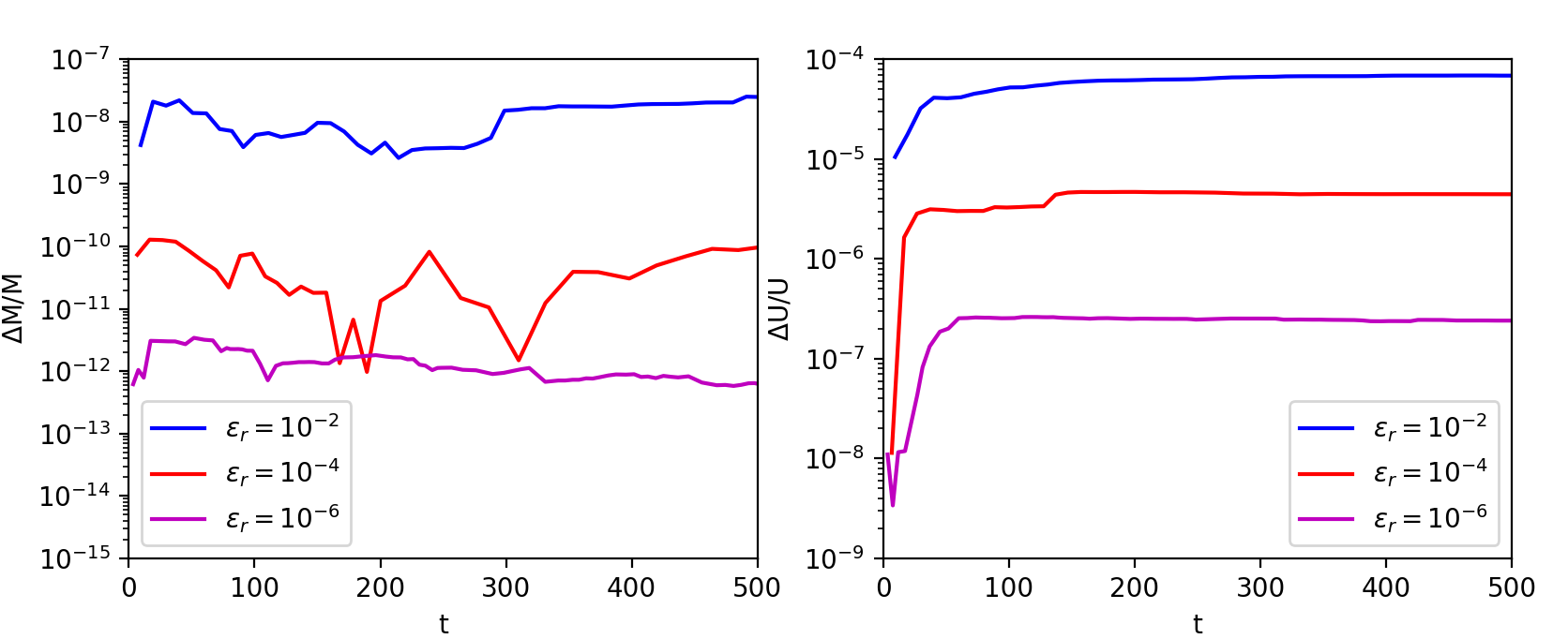
For this section, the time-step ramping discussed in Sec. 5.5 is not used to allow for a time-convergence study, and the first time-step size is taken to be Δ​tm​a​x10\frac{\Delta t_{max}}{10}. We demonstrate the discrete conservation theorem for mass and energy with a grid of Nξ×Nv|⁣|×Nv⟂=96×64×32N_{\xi}\times N_{v_{||}}\times N_{v_{\perp}}=96\times 64\times 32, a time-step size of Δ​tm​a​x=10−1\Delta t_{max}=10^{-1}, and varying nonlinear convergence tolerance of ϵr​e​l=10−2\epsilon_{rel}=10^{-2}, 10−410^{-4}, and 10−610^{-6}; refer to Fig. 2.

Refer to caption
Figure 2: Doubly reflective boundary problem with prescribed grid motion: Discrete conservation of mass and energy for varying nonlinear convergence tolerance.

As can be seen, discrete conservation error in mass, Δ​M(p)M(0)\frac{\Delta M^{(p)}}{M^{(0)}}, and energy, Δ​U(p)U(0)\frac{\Delta U^{(p)}}{U^{(0)}}, reduces commensurately with the nonlinear convergence tolerance. Here,

M(p)=∑αNsmα​∑i=1NξΔ​ξ​JS​ξ,i(0)​⟨1,f~α,i(p)⟩δ​𝐯,M^{(p)}=\sum_{\alpha}^{N_{s}}m_{\alpha}\sum_{i=1}^{N_{\xi}}\Delta\xi J_{S\xi,i}^{(0)}\left\langle 1,\widetilde{f}_{\alpha,i}^{(p)}\right\rangle_{\delta\mathbf{v}}, (90)
Δ​M(p)=|M(p)−M(0)|,\Delta M^{(p)}=\left|M^{(p)}-M^{(0)}\right|, (91)
U(p)=∑αNsmα​∑i=1NξΔ​ξ​JS​ξ,i(p)​⟨v22,f~α,i(p)⟩δ​𝐯+32​∑i=1NξΔ​ξ​JS​ξ,i(p)​ne,i(p)​Te,i(p),U^{(p)}=\sum_{\alpha}^{N_{s}}m_{\alpha}\sum_{i=1}^{N_{\xi}}\Delta\xi J_{S\xi,i}^{(p)}\left\langle\frac{v^{2}}{2},\widetilde{f}_{\alpha,i}^{(p)}\right\rangle_{\delta\mathbf{v}}+\frac{3}{2}\sum_{i=1}^{N_{\xi}}\Delta\xi J_{S\xi,i}^{(p)}n_{e,i}^{(p)}T_{e,i}^{(p)}, (92)

and

Δ​U(p)=|U(p)−U(0)|.\Delta U^{(p)}=\left|U^{(p)}-U^{(0)}\right|. (93)

Next, we demonstrate the discretization order of convergence of the proposed algorithm. The temporal, configuration-space, and velocity-space convergence study is performed by measuring the L2L_{2}-norm of the relative difference of the temperature,

ℰTΔ​t=∑i=1NξΔ​ξ​[∑α=1Ns​p(Tα,iΔ​t−Tα,iΔ​tr​e​f)2+(Te,iΔ​t−Te,iΔ​tr​e​f)2],{\cal E}_{T}^{\Delta t}=\sqrt{\sum_{i=1}^{N_{\xi}}\Delta\xi\left[\sum_{\alpha=1}^{N_{sp}}\left(T_{\alpha,i}^{\Delta t}-T_{\alpha,i}^{\Delta t_{ref}}\right)^{2}+\left(T_{e,i}^{\Delta t}-T_{e,i}^{\Delta t_{ref}}\right)^{2}\right]}, (94)
ℰTΔ​ξ=∑i=1NξΔ​ξ​[∑α=1Ns​p(Tα,iΔ​ξ−Tα,iΔ​ξr​e​f)2+(Te,iΔ​ξ−Te,iΔ​ξr​e​f)2],{\cal E}_{T}^{\Delta\xi}=\sqrt{\sum_{i=1}^{N_{\xi}}\Delta\xi\left[\sum_{\alpha=1}^{N_{sp}}\left(T_{\alpha,i}^{\Delta\xi}-T_{\alpha,i}^{\Delta\xi_{ref}}\right)^{2}+\left(T_{e,i}^{\Delta\xi}-T_{e,i}^{\Delta\xi_{ref}}\right)^{2}\right]}, (95)
ℰTΔ​v~=∑i=1NξΔ​ξ​[∑α=1Ns​p(Tα,iΔ​v~−Tα,iΔ​v~r​e​f)2+(Te,iΔ​v~−Te,iΔ​v~r​e​f)2].{\cal E}_{T}^{\Delta\widetilde{v}}=\sqrt{\sum_{i=1}^{N_{\xi}}\Delta\xi\left[\sum_{\alpha=1}^{N_{sp}}\left(T_{\alpha,i}^{\Delta\widetilde{v}}-T_{\alpha,i}^{\Delta\widetilde{v}_{ref}}\right)^{2}+\left(T_{e,i}^{\Delta\widetilde{v}}-T_{e,i}^{\Delta\widetilde{v}_{ref}}\right)^{2}\right]}. (96)

Here, the superscript Δ​t\Delta t denotes the solution obtained with a larger time-step size while Δ​tr​e​f\Delta t_{ref} denotes the reference solution, Δ​ξ\Delta\xi denotes the solution obtained with a coarse logical space grid size and Δ​ξr​e​f\Delta\xi_{ref} denotes the reference solution, and Δ​v~\Delta\widetilde{v} denotes the solution obtained with a coarse velocity-space grid and Δ​v~r​e​f\Delta\widetilde{v}_{ref} denotes the reference grid.

The temporal discretization relies on a BDF2 scheme and is second order accurate (refer to Fig. 3-left). We compute the L2L_{2}-norm of the relative difference of the temperatures. The reference solution uses a grid of Nξ=24N_{\xi}=24, Nv|⁣|=32N_{v_{||}}=32, Nv⟂=16N_{v_{\perp}}=16, and a time-step size of Δ​tr​e​f=10−3\Delta t_{ref}=10^{-3}, and is time integrated to tm​a​x=0.25.t_{max}=0.25. The convergence study is performed by fixing the grids while varying the time-step size.

The configuration-space discretization relies on a SMART discretization for the flux interpolation, which asymptotically is third order accurate. However, we see in Fig. 3-center that we recover only second-order accuracy. This is due to the second-order accurate operations employed elsewhere (e.g., linear interpolation employed for the configuration-space cell-face quantities [e.g., Jr2,J_{r^{2}}, JξJ_{\xi}, v∗v^{*}, u|⁣|∗u_{||}^{*}] as well as cell-face evaluation of the gradients [second order centered differencing] of velocity-space metrics [e.g., ∂ξv∗\partial_{\xi}v^{*} and ∂ξu|⁣|∗\partial_{\xi}u_{||}^{*}]). We note that the solution in the physical space is compared by interpolating the reference solution to the coarse grid. The reference solution uses a grid of Nξ=384N_{\xi}=384, Nv|⁣|=32N_{v_{||}}=32, Nv⟂=16N_{v_{\perp}}=16, and a time-step size of Δ​t=0.025\Delta t=0.025 and is time integrated to tm​a​x=0.25.t_{max}=0.25. The convergence study is performed by fixing the time-step size and velocity-space resolution while varying the number of configuration-space grid points.

Similarly to the configuration space, the velocity-space discretization also relies on the SMART scheme for the flux interpolation. However, due to the linear interpolation used elsewhere (e.g., interpolation of advection coefficients to the cell face), the overall discretization is second order as is seen in Fig. 3-right. The reference solution uses a grid of Nξ=24N_{\xi}=24, Nv|⁣|=512N_{v_{||}}=512, Nv⟂=256N_{v_{\perp}}=256, a time-step size of Δ​t=0.025\Delta t=0.025, and time integrated to tm​a​x=0.25.t_{max}=0.25. The convergence study is performed by fixing the time-step size and configuration-space grid while uniformly refining the transformed velocity-space grid in both v~|⁣|\widetilde{v}_{||} and v~⟂\widetilde{v}_{\perp}.

Refer to caption
Refer to caption
Refer to caption
Figure 3: Doubly reflective boundary problem with prescribed grid motion: Temporal (left), configuration-space (center), and velocity-space (right) convergence study. As can be seen, second order convergence rate is observed in all discretization parameters.

6.2 Guderley problem (time-dependent Maxwellian Dirichlet boundary conditions)

We consider the Guderley problem [78, 79, 80, 81] of a converging/diverging shock to test the proposed time-dependent boundary conditions in spherical geometry and to demonstrate the ability of the algorithm to capture the hydrodynamic asymptotic limit for short mean-free-paths. Semi-analytic solutions to the Euler equations exist for the Guderley problem (see I for details), which we will appeal to for verification. Suppose that a strong shock is spherically converging into a uniform, Deuterium-Tritium, ⟨DT⟩\langle\text{DT}\rangle, plasma with constant mass density of ρ0=m⟨D​T⟩​n⟨D​T⟩=0.173\rho_{0}=m_{\left\langle DT\right\rangle}n_{\left\langle DT\right\rangle}=0.173 [g/c​cg/cc] and temperature T0=10T_{0}=10 [e​VeV] (i.e., conditions relevant to double-shell and revolver ICF implosions[82, 83, 84, 85, 86, 87, 88, 89, 90, 91]). We model the ⟨DT⟩\langle\text{DT}\rangle plasma as an equimolar, averaged single ion, fully ionized, and initialize the distribution function with density, drift velocity, and pressure/temperature profiles obtained from a Guderley solution. The Guderley profiles are obtained 20 [p​sps] after the shock was initialized from a radius of R0=200R_{0}=200 [μ​m\mu m], and the Mach number there is M0=7.23M_{0}=7.23. Similarly, the hydrodynamic boundary conditions for the spherical domain are sourced from the same Guderley solution. The logical grid sizes for these calculations are chosen as Nξ=N_{\xi}=192 and 384, Nv⟂=64N_{v_{\perp}}=64 and Nv|⁣|=128N_{v_{||}}=128 with domain limits ξ×v~|⁣|×v~⟂∈[0,1]×[−8,8]×[0,8]\xi\times\widetilde{v}_{||}\times\widetilde{v}_{\perp}\in\left[0,1\right]\times\left[-8,8\right]\times\left[0,8\right]. The profiles for the initial and the boundary conditions for the moments are shown in Fig. 4.

Refer to caption
Figure 4: Guderley problem: The initial condition (top) and the time-dependent Maxwellian boundary conditions (bottom) for the number density (left), radial drift velocity (center), and temperature (right), obtained from semi-analytically solving the Guderley problem in Ref. [79]. For the initial condition, the black markers denotes the grid density (i.e., coarse grid regions are lighter in color than finer regions). The boundary temperature is assumed to be equilibrated across ions and electrons at all time.

We start our verification study by employing a static and uniform mesh in the configuration space (while keeping the the velocity-space mesh adaptive). The purpose of this case is to serve as the baseline to highlight the computational savings and the accuracy gains afforded by the fully adaptive phase-space mesh. For the verification metric, we choose the shock speed,

us=|d​rsd​t|,u_{s}=\left|\frac{dr_{s}}{dt}\right|, (97)

where rsr_{s} is the shock position. The simulated shock trajectory is defined either as: 1) the location of the maximum ion temperature, or 2) the location of the maximum ion viscous (energy) dissipation rate. The first definition is the most reliable (i.e., it has less dependence on small-scale fluctuations in the moment quantities), but only unambiguously identifies the shock location in the converging phase. For our simulations, we choose definition 1 for the converging shock phase, and 2 for the diverging phase. We define the viscous dissipation rate as:

(d​Tid​t)visc=−23​(τ||||ni)​∂r(r2u||,i)r2,\left(\frac{dT_{i}}{dt}\right)_{\text{visc}}=-\frac{2}{3}\left(\frac{\tau_{||||}}{n_{i}}\right)\frac{\partial_{r}\left(r^{2}u_{||,i}\right)}{r^{2}}, (98)

where, TiT_{i} is the ion temperature, u||,iu_{||,i} is the radial component of the ion drift velocity, nin_{i} is the total ion number density, and τ||||\tau_{||||} is the radial component of the ion viscosity tensor [Eq. (63)]. Fig. 5-left shows a comparison of the shock speed versus time for the two different spatial-grid resolutions. The two curves show strong deviations from each other near the shock collapse time of approximately 500 [ps]. The noticeable fluctuations in the curves suggest that the simulations are poorly resolving the shock structure, where the spatial gradients can change dramatically in the course of the shock’s collapse.

Figure 5: Guderley problem: The shock speed versus time with a static and uniform configuration-space grid (left) and a moving mesh with an optimized initial mesh generation (right).

We see a dramatic improvement in the quality of the solution when we employ an initial grid optimization in conjunction with the NS-MMPDE strategy with δm​i​n=5×10⁻³\delta_{min}=5\times 10^{-3} and λω=10−3\lambda_{\omega}=10^{-3}. Indeed, as shown in Fig. 5-right, the differences between Nξ=192N_{\xi}=192 and Nξ=384N_{\xi}=384 disappear, and the fluctuations seen in Fig. 5-left are nearly eliminated for both cases. Moreover, comparing the static and the moving mesh cases for Nξ=384N_{\xi}=384 reveals the origin of the deviations in the shock trajectory near the collapse time: As seen in Fig. 6, the shock trajectory with the uniform mesh veers away from the correct trajectory immediately after the simulation begins.

Figure 6: Guderley problem: The shock speed versus time comparing the two simulations for Nξ=384N_{\xi}=384. Green (solid) uses a static and uniform configuration-space mesh and magenta (dashed) uses NS-MMPDE.

The initial shock structure is not well resolved in the static-mesh simulation, and this seems to be the cause of the strong deviation. The drifting Maxwellian for the temperature, density, and drift velocity are not the true distribution functions for the shock, and this leads to the production of transients in the solution which, if not properly resolved, can cause the solution to deviate strongly from initial condition.

We expect that such a high ⟨DT⟩\langle\text{DT}\rangle density (0.1730.173 [g/c​cg/cc]) justifies the use of boundary conditions sourced from a dissipation-less fluid theory (i.e., Euler equations), and that a meaningful comparison to this theory is actually possible. To this end, we compare our Nξ=192N_{\xi}=192 NS-MMPDE results to the corresponding Guderley solution. Fig. 7-left shows the shock trajectory as a function of time from the simulation and the semi-analytic Guderley prediction. We see that the shock collapse times agree very well. Remarkably, the Guderley shock collapse time and the simulation agree to within 0.75%0.75\%.

Figure 7: Guderley problem: The shock trajectory vs. time. The blue (“solid”) curve is obtained from our algorithm for Nξ=192N_{\xi}=192 with the proposed NS-MMPDE and initial grid optimization algorithms, and the red (“dashed”) curve is the semi-analytical Guderley prediction over the entire simulation (left) and the isolated time in the vicinity of the shock collapse (right).

However, if we take a closer look in the neighborhood of the collapse, as depicted in the “zoomed in” trajectory plot shown in Fig. 7-right, we see that the Guderley and simulated shock trajectories differ in the early post-collapse phase. Insight into this discrepancy may be gained by directly comparing the simulation and Guderley hydrodynamic profiles. Fig. 8-top shows pre-collapse profiles for density (left), drift velocity (center), and total hydrodynamic pressure, P=ni​Ti+ne​TeP=n_{i}T_{i}+n_{e}T_{e} (right). We see that there is some separation between the simulation and Guderley densities at an early time (t = 100 [p​sps] after the simulation is initialized). Moreover, the transients created in the simulation initialization have yet to be fully eliminated. By t = 400 [p​sps], however, the simulation and Guderley profiles largely agree, although we see some remaining differences near the shock collapse time (t = 552.5 [p​sps]), which persist into the diverging phase – as depicted in Fig. 8-bottom. Nevertheless, the qualitative features are nearly identical between simulation and Guderley.

Figure 8: Guderley problem: Pre-collapse (top) and post-collapse (bottom) hydro profiles for number density (left), drift velocity (center), and total hydrodynamic pressure (right) from simulation (“solid”) and Guderley (“dashed”).

The strong deviations in the hydro profiles seen in Fig. 8-bottom hint at the origin of the trajectory discrepancy in the post-collapse phase – as shown in Fig. 7-right. The Guderley solution predicts a zero density and (infinite temperature) at the origin at the shock collapse time. This behavior is unphysical, and it results from the infinite collisionality assumption in the Euler equations [80]. The VFP equation models the full dissipation physics, and thus captures the correct behavior near shock collapse (where ion heat conduction, viscosity, and kinetic effects become important).

In Fig. 9 we show, as a function of time, the max⁡(Δ​r)/min⁡(Δ​r)\max\left(\Delta r\right)/\min\left(\Delta r\right) and ⟨Δ​r⟩/min⁡(Δ​r)\left\langle\Delta r\right\rangle/\min\left(\Delta r\right) (where ⟨Δ​r⟩=∑i=1NξΔ​ri/Nξ\left\langle\Delta r\right\rangle=\sum_{i=1}^{N_{\xi}}\Delta r_{i}/N_{\xi}) to demonstrate the computational complexity reduction (relative to a uniform grid) afforded by the proposed NS-MMPDE scheme.

Figure 9: Guderley problem: Ratios of maximum to minimum (left) and average to minimum (right) grid sizes versus time.

As can be seen, both ratios exhibit large values and a reduction of approximately 20 in the computational complexity is achieved by the mesh motion for the Guderley problem. In Fig. 10, a Lagrangian radius-time (RT) diagram of 1/Δ​r1/\Delta r is shown to demonstrate how the grid tracks the shock front as a function of time.

Refer to caption
Figure 10: Guderley problem: RT diagram of 1/Δ​r1/\Delta r for Nξ=192N_{\xi}=192.

As can be seen, the grid tightly concentrates near the sharp converging shock front, and diffuses away after shock collapse due to kinetic effects smearing the gradients. Finally, to demonstrate the computational complexity reduction afforded by the velocity-space adaptivity scheme, we present the parallel velocity-space marginal distribution function,

f||,<DT>=2π∫0∞dv⟂v⟂f⟨D​T⟩,f_{||,<DT>}=2\pi\int_{0}^{\infty}dv_{\perp}v_{\perp}f_{\left\langle DT\right\rangle}, (99)

in the r−v|⁣|r-v_{||} plane in Fig. 11.

Refer to caption
Refer to caption
Refer to caption
Refer to caption
Figure 11: Guderley problem: Parallel velocity-space marginal distribution functions at t≈0, 200,550, 700t\approx 0,\;200\;,550,\;700 [ps].

For the calculation, max⁡(vt​h)/min⁡(vt​h)≈15,\max\left(v_{th}\right)/\min\left(v_{th}\right)\approx 15, thus a total computational complexity reduction of max\max (⟨Δ​r⟩min⁡(Δ​r))\left(\frac{\left\langle\Delta r\right\rangle}{\min\left(\Delta r\right)}\right) (max⁡(vt​h)min⁡(vt​h))2\left(\frac{\max\left(v_{th}\right)}{\min\left(v_{th}\right)}\right)^{2} ≈4500\approx 4500 is achieved through the moving phase-space mesh strategy. We stress that, due to the large velocity scales encountered in the problem, it is not possible to simulate the present problem on a static and uniform velocity-space grid. We remind the readers that this problem is intended to be a verification of the proposed numerical method to recover the hydrodynamic solution and that to our knowledge, these results are unprecedented for a kinetic code. Because of the nature of the problem, kinetic effects are not significant and the true capability of the proposed algorithm is highlighted later in a multi-scale ICF capsule implosion simulation (Sec. 6.4), where kinetic physics manifest in a non-trivial manner.

6.3 Van Dyke problem (elastic moving wall boundary condition)

Consider a spherical piston surrounding a gas at constant pressure and density. At t=0t=0, the piston begins moving at a constant velocity inward. A shock is created in the gas, and converges to the center. We simulate this setup directly, using the moving elastic wall boundary condition discussed in Sec. 5.4.1. Once more, we consider a fully ionized ⟨DT⟩\langle\text{DT}\rangle gas with an initial mass density of ρ⟨D​T⟩=m⟨D​T⟩​n⟨D​T⟩=0.173\rho_{\left\langle DT\right\rangle}=m_{\left\langle DT\right\rangle}n_{\left\langle DT\right\rangle}=0.173 [g/c​cg/cc] and temperature of T⟨D​T⟩=10T_{\left\langle DT\right\rangle}=10 [e​VeV]. The piston velocity was chosen to be uW=−19u_{W}=-19 [c​m/μ​scm/\mu s] inwards, and the initial radius was R0=326R_{0}=326 [μ​m\mu m]. To avoid any violent, abrupt changes in the ion distribution function at the wall, we accelerate the wall to the desired piston velocity (-19 [c​m/μcm/\mus]) at a constant rate. Considering two different acceleration times (2.5 and 5 [p​sps]), we found negligible differences in the final solution. Our convergence study begins with a static mesh (Nξ=192N_{\xi}=192; Nv⟂=64N_{v_{\perp}}=64; Nv|⁣|=128N_{v_{||}}=128).

This simulation predicted a shock collapse time of 938 [ps], which is 30 [p​sps] later than the Van Dyke prediction [92] of 908 [p​sps]. Nonetheless, this is only about a 3%3\% difference. The collapse time further improves when we use the NS-MMPDE algorithm, going from 938→928938\rightarrow 928 [p​sps]. This figure is largely insensitive to the grid resolution, and the non-linear convergence tolerance; changing only to 927 [p​sps] for Nξ=384N_{\xi}=384 (keeping all other parameters constant), and 930 [p​sps] when Nξ=192N_{\xi}=192 and the relative tolerance is changed from ϵr​e​l=10−2\epsilon_{rel}=10^{-2} to ϵr​e​l=​10−3\text{$\epsilon_{rel}=$}10^{-3}. The largest gain was attained by enhancing the grid resolution near the piston using an initial grid optimization. We once more used Nξ=192N_{\xi}=192. In this case, the simulated collapse time was 909 [p​sps], putting the agreement with the Van-Dyke solution within ≈0.1%\approx 0.1\%. Fig. 12-left shows that this is not just a coincidence; the simulated shock trajectory precisely matches that of Van Dyke.

Figure 12: Van Dyke problem: The shock trajectory versus time. The blue (“solid”) curve is obtained from simulation using the elastic moving wall boundary condition, and the red (“dashed”) curve is the Van Dyke (left) and Guderley (right) predictions.

Finally, the Van Dyke solution asymptotically approaches the Guderley solution as the shock collapses. Fig. 12-right shows decent agreement between simulation and the equivalent Guderley-shock trajectories. As before, we can also compare the numerical and Guderley hydro profiles. Figs. 13-top shows pre-collapse profiles for density (left), drift velocity (center), and total hydrodynamic pressure (right). Similarly to the time-dependent boundary condition simulations in Section 6.2, the simulation and Guderley profiles agree exceedingly well. The shock collapse times agree within 0.02%0.02\%. Nevertheless, Figs. 13-bottom show that significant differences remain in the post-collapse profiles.

Figure 13: Van Dyke problem: Pre-collapse (top) and post-collapse (bottom) hydro profiles for density (left), drift velocity (center), and total hydrodynamic pressure (right) – given the moving wall boundary condition – from simulation (“solid”) and Guderley (“dashed”).

This is believed to be due to the finite kinetic effects near shock collapse time inducing wall heating of the plasma and altering the dynamics of the reflected shock. Further, since the Guderley problem is strictly only applicable for an infinite domain, the solutions continue to deviate as the wall comes closer to the diverging shock front.

Similarly to the Guderley problem, we demonstrate the grid savings in the configuration space by showing the maximum- and average-to-minimum grid size ratios in Fig. 14.

Refer to caption
Figure 14: Van Dyke problem: Ratios of maximum to minimum (left) and average to minimum (right) grid sizes versus time.

As can be seen, a complexity reduction in configuration space of roughly 50 is achieved for the Van Dyke problem. Further, since max⁡(vt​h)/min⁡(vt​h)≈15,\max\left(v_{th}\right)/\min\left(v_{th}\right)\approx 15, a total computational complexity reduction of max⁡(⟨Δ​r⟩min⁡(Δ​r))​(max⁡(vt​h)min⁡(vt​h))2≈11250\max\left(\frac{\left\langle\Delta r\right\rangle}{\min\left(\Delta r\right)}\right)\left(\frac{\max\left(v_{th}\right)}{\min\left(v_{th}\right)}\right)^{2}\approx 11250 is achieved through the moving phase-space grid strategy. In Fig. 15, a Lagrangian RT diagram of 1/Δ​r1/\Delta r to demonstrate how the grid tracks the shock front as a function of time.

Refer to caption
Figure 15: Van Dyke problem: RT diagram of 1/Δ​r1/\Delta r for Nξ=192N_{\xi}=192.

As can be seen, the grid tracks several shock reflections from the center and the wall, until gradients broaden due to finite transport effects and the grid relaxes. Finally, in Fig. 16 we demonstrate the discrete mass conservation [from conservation theorems in Eqs. (49) - (53)] for the elastic moving wall boundary condition.

Refer to caption
Figure 16: Van Dyke problem: Relative mass difference as a function of time.

As can be seen, the total mass variation is well below the relative nonlinear convergence tolerance of ϵr=10−3\epsilon_{r}=10^{-3} as designed.

6.4 Fuel-only compression yield simulation of shot 22862 at the Omega Facility (pressure-driven Lagrangian boundary condition)

We reproduce the results reported in Ref. [52] in which a fuel-only simulation was performed for a compression yield target to study the so-called Rygg effect [5, 7, 52]. We consider this problem for three reasons: 1) to test the implementation of the pressure-driven Lagrangian boundary conditions on a realistic implosion experiment; 2) to demonstrate the performance of our nonlinear solver strategy applied to a realistic implosion scenario; and 3) to demonstrate the algorithmic advantage of our proposed NS-MMPDE scheme over the classic MMPDE scheme.

The Rygg effect refers to the anomalous (non-hydrodynamic) scaling of experimental yield observed by Ref. [5]. In the reference, experiments were performed to test the validity of the hydrodynamic assumptions in a plastic (CH) capsule with D-3He filled capsules at the Omega laser ICF facility. In the experiments, the fuel species concentrations were varied from shot to shot such that the initial mass density, ρ=∑αNsmα​nα\rho=\sum_{\alpha}^{N_{s}}m_{\alpha}n_{\alpha}, and total hydrodynamic pressure, P=∑αNs(1+Zα)​nα​TαP=\sum_{\alpha}^{N_{s}}\left(1+Z_{\alpha}\right)n_{\alpha}T_{\alpha}, was kept fixed, thus ensuring hydro-equivalence. Here, mD=2​mpm_{D}=2m_{p}, mH3​e=3​mpm_{{}^{3}He}=3m_{p} and ZαZ_{\alpha} is the ionization state of ion-species α\alpha. Accordingly, if hydrodynamic predictions are valid, the nuclear yield of D-D reaction, YD​D∝nD2Y_{DD}\propto n_{D}^{2}, should follow a simple fD2f_{D}^{2} scaling law, where fDf_{D} is the deuterium number fraction, defined as:

fD=nDnD+nH​e​3.f_{D}=\frac{n_{D}}{n_{D}+n_{He3}}. (100)

The hydrodynamic variables were obtained from the LILAC Lagrangian rad-hydro simulation for Omega facility experimental shot 22862 at the last fuel region. The simulation was initialized at t0=500.5t_{0}=500.5 [p​sps] at the moment in which the shock breaks out of the fuel-pusher interface; refer to Fig. 17. We note that at this point the fuel species’, Deuterium and Helium-3, are assumed to be fully ionized (ZD=1Z_{D}=1 and ZH3​e=2Z_{{}^{3}He}=2).

Refer to caption
Refer to caption
Figure 17: Fuel-only compression yield simulation: The initial condition (top) and the time-dependent Maxwellian boundary conditions (bottom) for the number density, nn, radial drift velocity, uu, and temperature, TT, obtained from the LILAC rad-hydro calculation for the last Lagrangian fuel zone at the time in which the first shock breaks out of the fuel-pusher interface (~500.5 [p​sps]). For the initial condition for number densities, the blue (red) curve denotes Deuterium (Helium-3); for the temperature, blue (green) denotes ions (electrons); and the black markers denotes the grid density (i.e., coarse grid regions are lighter in color than finer regions). We remind the readers that the boundary position and velocity are evolved from the mass conservation constraint and the Lagrangian equation of motion [Eqs. (57) and 59], respectively, and are not explicitly provided to drive the simulation. Further the boundary temperatures and drift velocities are assumed to be equilibrated across species at all times.

We consider a grid of Nξ=96N_{\xi}=96, Nv|⁣|=128N_{v_{||}}=128, Nv⟂=64N_{v_{\perp}}=64, and a transformed velocity-domain size of v~|⁣|∈[−6,6]\widetilde{v}_{||}\in\left[-6,6\right] and v~⟂∈[0,6]\widetilde{v}_{\perp}\in\left[0,6\right] with grid parameters, λv∗=λu∗=10−3\lambda_{v^{*}}=\lambda_{u^{*}}=10^{-3}, δm​i​n=0.025\delta_{min}=0.025, λω=10−3\lambda_{\omega}=10^{-3}, τr=0.1\tau_{r}=0.1 [p​sps], and Δ​tm​a​x=0.2\Delta t_{max}=0.2 [p​sps]. In Fig. 18, the simulation results are shown for the case of fD=0.5f_{D}=0.5 at the beginning of the simulation, upon shock collapse, and at peak compression.

Refer to caption
Figure 18: Fuel-only compression yield simulation: The density (top), drift velocity (center), and temperature (bottom) for the fD=0.5f_{D}=0.5 case prior to shock convergence (~1450 [p​sps]), upon shock reflection (~1650 [p​sps]) and at near peak compression and stagnation (~2050 [p​sps]). The black markers denotes the grid density.

As can be seen, an appreciable fuel separation is seen in all quantities at shock collapse time (~1450[p​sps]). The separations are supported due to the difference in vt​h=2​T/mv_{th}=\sqrt{2T/m} amongst the ion species and the long D-3He mean-free-paths –which scales as λD−3He∝T2/(ZD2ZH3​e2)\lambda_{D-^{3}He}\propto T^{2}/\left(Z_{D}^{2}Z_{{}^{3}He}^{2}\right)– supported within the shock; refer to Fig. 19.

Refer to caption
Refer to caption
Figure 19: Fuel-only compression yield simulation: The temperature (top) of the various plasma species, and the corresponding ion marginal parallel-velocity distribution function (bottom) for Deuterium (left) and Helium-3 (right).

As can be seen, a distinct beam feature forms in the Deuterium species, allowing a significant population to run ahead of the Helium-3. These structures are inherently kinetic and far from a linear perturbation in pitch angle, necessitating a general description for the distribution function. In fact, one observes that the plasma near the shock front is appreciably kinetic throughout the entire course of the implosion process as can be seen in the Knudsen number RT diagram in Fig. 20.

Refer to caption
Figure 20: Fuel-only compression yield simulation: The Deuterium Knudsen number RT diagram is shown. Here, the Knudsen number is defined as K​n=vt​h,D​τe​f​f​∂rln⁡ni​o​nKn=v_{th,D}\tau_{eff}\partial_{r}\ln n_{ion}, where ni​o​n=nD+nh3​en_{ion}=n_{D}+n_{{}^{3}he}, vt​h,D=2​TD/mDv_{th,D}=\sqrt{2T_{D}/m_{D}}, τe​f​f=(τD​D−1+τD3​H​e−1+τD​e−1)−1\tau_{eff}=\left(\tau_{DD}^{-1}+\tau_{D^{3}He}^{-1}+\tau_{De}^{-1}\right)^{-1}, and τD​β∝Tβ3/2/(ZD2​Zβ2​nβ​mβ1/2)\tau_{D\beta}\propto T_{\beta}^{3/2}/\left(Z_{D}^{2}Z_{\beta}^{2}n_{\beta}m_{\beta}^{1/2}\right). As can be seen, the Knudsen number is relatively large near the shock trajectory while at peak compression, it reduces to below 10−310^{-3}.

As seen, although the Knudsen number does reduce to K​n≤10−3Kn\leq 10^{-3} at peak-compression time, hence equilibrating the distribution function roughly to a Maxwellian, the early separation in the species densities persists due to the early kinetic imprinting in the solution. As a consequence, Deuterium species are depleted from the hot core and transported to the periphery of the domain, leading to a degradation in the D-D yield.

In Fig. 21 the normalized (to the fD=1f_{D}=1 case) D​DDD-neutron nuclear yield,

Y~D​DfD=YD​DfDYD​DfD=1​(nDfD=1nDfD)2,\widetilde{Y}_{DD}^{f_{D}}=\frac{Y_{DD}^{f_{D}}}{Y_{DD}^{f_{D}=1}}\left(\frac{n_{D}^{f_{D}=1}}{n_{D}^{f_{D}}}\right)^{2}, (101)

is shown, where

YD​D=2​π​∫t0tm​a​xd​t​∫r2​𝑑r​∫d3​v​fD​(r,𝐯)​∫d3​v′​fD​(r,𝐯′)​|𝐯−𝐯′|​g​(|𝐯−𝐯′|),Y_{DD}=2\pi\int_{t_{0}}^{t_{max}}dt\int r^{2}dr\int d^{3}vf_{D}\left(r,\mathbf{v}\right)\int d^{3}v^{\prime}f_{D}\left(r,\mathbf{v}^{\prime}\right)\left|\mathbf{v}-\mathbf{v}^{\prime}\right|g\left(\left|\mathbf{v}-\mathbf{v}^{\prime}\right|\right), (102)

g⁡(|𝐯−𝐯′|)g\left(\left|\mathbf{v}-\mathbf{v}^{\prime}\right|\right) is the D​D−nDD-n cross section [93], and nDfDn_{D}^{f_{D}} is the initial (un-shocked) Deuterium number density for a given fDf_{D}.

Refer to caption
Figure 21: Fuel-only compression yield simulation: Y~D​DfD\widetilde{Y}_{DD}^{f_{D}} for varying fD0f_{D}^{0}. The blue markers denote values obtained in this study, while the reference values obtained from Ref. [52] are shown in red. We note that the observed disagreement with the reference result is expected due to the significant algorithmic improvements we have made to iFP (e.g., improved treatment for the phase-space grid adaptivity, dynamic time-step adaptivity, etc.)

As can be seen, with decreasing fDf_{D} (increasing fH​e​3f_{He3}), the scaled relative yield decreases. In a single-fluid hydrodynamic formalism, the total mass and pressure would be independent of species concentrations, leading to no variation in Y~D​Df​D\widetilde{Y}_{DD}^{fD}. In kinetic theory however, differential-ion motion, viscous heating, and other kinetic physics break hydro-equivalence and lead to dependence of Y~D​DfD\widetilde{Y}_{DD}^{f_{D}} with Deuterium concentration. For further insights and discussion into the yield variation physics, we refer the reader to Ref. [52].

In Fig. 22, we demonstrate the performance of our solver strategy by showing, for the fD=0.5f_{D}=0.5 case, the instantaneous number of outer fixed-point/nonlinear iteration (i.e., number of evaluation of the fixed point map summarized in Alg. 2) as a function of time.

Refer to caption
Figure 22: Fuel-only compression yield simulation: Instantaneous number of outer fixed point iteration, NN, versus time (blue) and the same quantity with a single pass of binomial smoothing (red), N∗,(p)=N(p+1)+2​N(p)+N(p−1)4N^{*,(p)}=\frac{N^{(p+1)}+2N^{(p)}+N^{(p-1)}}{4}, where the superscript (*) denotes the smoothed value, and (p) denotes the time-index.

As can be seen, the majority of the time-steps feature a reasonable number of iterations with an average over the entire simulation at approximately 5. A noticeable exception is in the 1000≤t≤14001000\leq t\leq 1400 [p​sps] time interval, where nontrivial structures are evolving in the simulation (e.g., second shock launched into the system, interaction and merging of the two shocks, and the subsequent fast evolution of physical structures), leading to occasional spikes in the number of nonlinear iterations. However, as can be seen from a single pass of binomial smoothing, the times in which the nonlinear iteration exceeds 10 is rare.

Further, once again for the fD=0.5f_{D}=0.5 case, we show the larger Δ​t\Delta t afforded by the NS-MMPDE scheme (relative to the standard MMPDE) by comparing the instantaneous Δ​t\Delta t as a function of time; refer to Fig. 23.

Refer to caption
Figure 23: Fuel-only compression yield simulation: Instantaneous Δ​t\Delta t versus time for NS-MMPDE and MMPDE (τr=0.1, 1, 10\tau_{r}=0.1,\;1,\;10 [ps]) for various grid relaxation time-scales. For the standard MMPDE, τr=0.1\tau_{r}=0.1 (blue) and 11 [ps] (red) cases lead to unstable time-integration as can be seen with the algorithm producing impractically small Δ​t\Delta t.

As seen, the NS-MMPDE scheme permits a generally larger Δ​t\Delta t with less erratic behavior than the standard MMPDE approach. The erratic behavior of MMPDE is attributed to the periodic jitter in the grid caused by the traveling shock front, which occasionally causes the grid near the shock front to evolve rapidly [and consequently a smaller Δ​t\Delta t is taken according to Eq. (66)]. In fact, the erratic grid evolution eventually leads to very small Δ​t\Delta t, rendering the simulation impractical for engineering-scale simulations. The only stable integration for the classic MMPDE scheme is obtained for a τr=10\tau_{r}=10 [p​sps] case, where the grid evolution time-scale is set to be longer than the dynamical time-scales in the system. Even then, occasional erratic behaviors are seen at around 1725 [p​sps]. In contrast, the proposed NS-MMPDE scheme detects regions where the grid is evolving rapidly in the predictor stage and attempts to minimize it through the optimization procedure, leading to a more robust behavior in the time-integration throughout the simulation. Thus, the proposed NS-MMPDE scheme greatly relaxes the process of having to empirically tune the τr\tau_{r}. Finally, we demonstrate the discrete mass conservation property for the pressure-driven Lagrangian boundary condition [from conservation theorems shown in Eqs. (55)-(57)], as shown in Fig. 24.

Refer to caption
Figure 24: Fuel-only compression yield simulation: Relative total mass variation as a function of time.

As can be seen, the mass is conserved to within the nonlinear convergence tolerance of 10−310^{-3}.

7 Conclusions and Future Work

We have demonstrated a conservative (mass, energy) phase-space moving-grid strategy in a spherically imploding system with a variety of boundary conditions - relevant to modeling ICF capsule implosions. The phase-space grid-adaptivity algorithm leverages the work from Ref. [56] by adapting the velocity-space grid based on the instantaneous thermal speed and bulk flow of the individual plasma species (i.e., multiple velocity-space grid). In the configuration space, the grid is evolved based on the MMPDE formalism. To deal with strong shocks and complex features encountered in implosion problems, we have developed a nonlinear stabilization strategy for the classic MMPDE algorithm (NS-MMPDE). The approach nonlinearly stabilizes MMPDE against numerical instabilities that can arise based on a fixed grid relaxation time-scale, τr\tau_{r}. The strategy is based on splitting the grid evolution process in two stages: 1) predict the grid based on MMPDE; and 2) pass the predicted grid through a nonlinear constrained optimization stage which optimizes the grid against the predicted value and the volumetric rate change. Our fully implicit solver is based on a nested Anderson accelerated fixed point iteration strategy that efficiently deals with the nonlinear coupling between the kinetic ion and fluid electrons. We have demonstrated the capability of the NS-MMPDE strategy (coupled with the previous velocity-space adaptivity capability and the adaptive time-stepping strategy) to robustly simulate ICF implosion problems including the Guderley/Van-Dyke problem –as far as we are aware, the first to do so in the literature with a Vlasov-Fokker-Planck approach. We have also demonstrated with a realistic Omega implosion experiment the integrated capability of the proposed algorithm in effectively dealing with multi-length and -velocity scale problems. Future work will include the extension of the proposed capability to: 1) kinetic electron treatment by advancing the work performed by Ref. [57] to spherical geometry (e.g., kinetic electron and Ampère equations); 2) to multiple spatial dimensions (e.g., 2D3V) in a general curvilinear coordinate system; 3) couple with radiation transport physics; 4) couple with a high-order low-order (HOLO) algorithm [94, 95, 96, 97, 98] to step over the stiff collision time-scales when dense and cold ablators are included in the simulation. We note that all extensions have already been performed and will be documented in follow-on publications.

Acknowledgments

We greatly appreciate Dr. Brian J. Albright from LANL for the many helpful discussions and particularly suggestions regarding the physics applications for the proposed capability. We appreciate Dr. Olivier Larroche from CEA for providing the LILAC rad-hydro initial and boundary conditions that were used for the Rygg problem and the many helpful discussions regarding clarifications on the FPION and FUSE capabilities. We thank Dr. Hong Sio from the Lawrence Livermore National Laboratory for discussions in simulating exploding pusher capsules, which ultimately lead to the need for improving our mesh motion strategy (and the eventual development of the NS-MMPDE scheme). We also thank the anonymous referees, whose suggestions helped to make the manuscript easier to understand. This work was sponsored by the Metropolis Postdoctoral Fellowship for W.T.T. between the years 2015-2017, the Thermonuclear Burn Initiative of the Advanced Simulation and Computing Program between years 2018-2020, the revolver LDRD project for B.D.K for year 2019, and the Institutional Computing program at the Los Alamos National Laboratory. This work was performed under the auspices of the National Nuclear Security Administration of the U.S. Department of Energy at Los Alamos National Laboratory, managed by Triad National Security, LLC under contract 89233218CNA000001.

References

  • [1] Y. B. Zel’dovich and Y. P. Raizer, Physics of shock waves and high-temperature hydrodynamic phenomena. Dover Publications, INC., 2 ed., 1967.
  • [2] R. P. Drake, High-energy-density physics. Springer, 2 ed., 2018.
  • [3] S. Atzeni and J. Meyer-Ter-Vehn, Inertial Fusion: beam plasma interaction, hydrodynamics, dense plasma physics. Oxford Science Publications, 2004.
  • [4] A. Petschek and D. Henderson, “Influence of high-energy ion loss on DT reaction rate in laser fusion pellets,” Nucl. Fusion, vol. 19, pp. 1678–1680, 1979.
  • [5] J. R. Rygg, J. A. Frenje, C. K. Li, F. H. Seguin, and R. D. Petrasso, “Tests of the hydrodynamic equivalence of direct-drive implosions with different d2 and 3he mixtures,” Phys. Plasmas, vol. 13, p. 052702, 2006.
  • [6] L. Welser-Sherrill, D. A. Haynes, R. C. Mancini, J. H. Cooley, R. Tommasini, I. E. Golovkin, M. E. Sherrill, and S. W. Haan, “Inference of icf implosion and core mix using experimental data and theoretical mix modeling,” High Energy Dens. Phys., vol. 5, pp. 249–257, 2009.
  • [7] H. W. Hermann, J. R. Langenbrunner, J. M. Mack, J. H. Cooley, D. C. Wilson, S. C. Evans, T. J. Sedillo, G. A. Kyrala, S. E. Caldwell, and et al., “Anomalous yield reduction in direct-drive deuterium/tritium implosions due to 3he addition,” Phys. Plasmas, vol. 16, p. 056312, 2009.
  • [8] P. A. Amendt, S. C. Wilks, C. Bellei, C. K. Li, and R. D. Petrasso, “The potential role of electric fields and plasma barodiffusion on the inertial confinement fusion database,” Phys. Plasmas, vol. 18, p. 056308, 2011.
  • [9] A. Thomas, M. Tzoufras, A. Robinson, R. Kingham, C. Ridgers, M. Sherlock, and A. Bell, “A review of Vlasov-Fokker-Planck numerical modeling of inertial confinement fusion plasma,” J. Comput. Phys., vol. 231, pp. 1051–1079, 2012.
  • [10] T. Ma, P. K. Patel, N. Izumi, P. T. Springer, M. H. Key, L. J. Atherton, L. R. Benedetti, D. K. Bradley, D. A. Callahan, P. M. Celliers, and et al., “Onset of hydrodynamic mix in high-velocity, highly compressed inertial confinement fusion implosions,” Phys. Rev. Lett., vol. 111, p. 085004, 2013.
  • [11] C. Bellei, P. A. Amendt, S. C. Wilks, M. G. Haines, D. T. Casey, C. K. Li, R. Petrasso, and D. R. Welch, “Species separation in inertial confinement fusion fuels,” Phys. Plasmas, vol. 20, p. 012702, 2013.
  • [12] J. A. Baumgaertel, P. A. Bradley, S. C. Hsu, J. A. Cobble, P. Hakel, I. Tregillis, N. S. Krasheninnikova, T. J. Murphy, M. J. Schmitt, R. C. Shah, K. D. Obrey, S. Batha, H. Johns, T. Joshi, D. Mayes, R. C. Mancini, and T. Nagayama, “Observation of early shell-dopant mix in omega direct-drive implosions and comparisons with radiation-hydrodynamic simulations,” Phys. Plasmas, vol. 21, p. 052706, 2014.
  • [13] H. G. Rinderknecht, H. Sio, C. K. Li, A. B. Zylstra, M. J. Rosenber, P. Amendt, J. Delettrez, C. Bellei, J. A. Frenje, M. G. Johnson, and et al., “First observations of nonhydrodynamic mix at the fuel-shell interface in shock-driven inertial confinement implosions,” Phys. Rev. Lett., vol. 112, p. 135001, 2014.
  • [14] M. J. Rosenberg, H. G. Rinderknecht, N. M. Hoffman, P. A. Amendt, S. Atzeni, A. B. Zylstra, C. K. Li, F. H. Séguin, H. Sio, M. G. Johnson, J. A. Frenje, R. D. Petrasso, V. Y. Glebov, C. Stoeckl, W. Seka, F. J. Marshall, J. A. Delettrez, T. C. Sangster, R. Betti, V. N. Goncharov, D. D. Meyerhofer, S. Skupsky, C. Bellei, J. Pino, S. C. Wilks, G. Kagan, K. Molvig, and A. Nikroo, “Exploration of the transition from the hydrodynamic like to the strongly kinetic regime in shock-driven implosions,” Phys. Rev., vol. 112, p. 185001, 2014.
  • [15] G. Kagan and X. Tang, “Thermo-diffusion in inertially confined plasmas,” Phys. Lett. A, vol. 378, pp. 1531–1535, 2014.
  • [16] H. G. Rinderknecht, M. Rosenberg, C. Li, N. Hoffman, G. Kagan, A. Zylstra, H. Sio, J. A. Frenje, M. G. Johnson, F. Séguin, R. Petrasso, and et al., “Ion thermal decoupling and species separation in shock-driven implosions,” Phys. Rev. Lett., vol. 114, p. 025001, 2015.
  • [17] L. Yin, B. J. Albright, W. Taitano, E. L. Vold, L. Chacón, and A. N. Simakov, “Plasma kinetic effects on interfacial mix,” Phys. Plasmas, vol. 23, p. 112302, 2016.
  • [18] A. N. Simakov and K. Molvig, “Hydrodynamic description of an unmagnetized plasma with multiple ion species. ii. two and three ion species plasmas,” Phys. Plasmas, vol. 23, p. 032116, 2016.
  • [19] A. Le, T. J. T. Kwan, M. J. Schmitt, H. W. Herrmann, and S. H. Batha, “Simulation and assessment of ion kinetic effects in a direct-drive capsule implosion experiment,” Phys. Plasmas, vol. 23, p. 102705, 2016.
  • [20] H. Sio, J. Frenje, J. Katz, C. Stoeckl, D. Weiner, M. Bedzyk, V. Glebov, C. Sorce, M. G. Johnson, H. Rinderknecht, A. B. Zylstra, and et al., “A particle X-ray temporal diagnostic (PXTD) for studies of kinetic, multi-ion effects, and ion-electron equilibration rates in inertial confinement fusion plasmas at OMEGA,” Rev. Sci. Instrum., vol. 87, p. 11D701, 2016.
  • [21] B. D. Keenan, A. N. Simakov, W. T. Taitano, and L. Chacón, “Ion species stratification within strong shocks in two-ion plasmas,” Phys. Plasmas, vol. 25, p. 032103, 2018.
  • [22] B. D. Keenan, A. N. Simakov, L. Chacón, and W. T. Taitano, “Deciphering the kinetic structure of multi-ion plasma shocks,” Phys. Rev. E, vol. 96, p. 053203, 2017.
  • [23] A. N. Simakov, B. D. Keenan, W. T. Taitano, and L. Chacón, “Plasma ion stratification by weak planar shocks,” Phys. Plasmas, vol. 24, p. 092702, 2017.
  • [24] T. Joshi, P. Hakel, S. Hsu, E. Vold, M. Schmitt, N. Hoffman, R. Rauenzahn, G. Kagan, X. Tang, R. Mancini, Y. Kim, and H. Herrmann, “Observation and modeling of interspecies ion separation in inertial confinement fusion implosions via imaging x-ray spectroscopy,” Phys. Plasmas, vol. 24, p. 056305, 2017.
  • [25] E. Vold, L. Yin, W. Taitano, K. Molvig, and B. J. Albright, “Diffusion-driven fluid dynamics in ideal gases and plasmas,” Phys. Plasmas, vol. 25, p. 062102, 2018.
  • [26] H. G. Rinderknecht, P. Amendt, S. Wilks, and G. Collins, “Kinetic physics in ICF: present understanding and future directions,” Plasma Phys. Control. Fusion, vol. 60, p. 064001, 2018.
  • [27] H. Sio, J. Frenje, A. Le, S. Atzeni, T. Kwan, M. G. Johnson, G. Kagan, C. Stoeckl, C. Li, C. Parker, C. Forrest, and et al., “Observations of multiple nuclear reaction histories and fuel-ion species dynamics in shock-driven inertial confinement fusion implosions,” Phys. Rev. Lett., vol. 122, p. 035001, 2019.
  • [28] J. D. Sadler, Y. Lu, B. Spiers, M. W. Mayr, A. Savin, R. Wang, R. Aboushelbaya, K. Glize, R. Bingham, H. Li, K. A. Flippo, and P. A. Norreys, “Kinetic simulation of fusion ignition with hot-spot ablator mix,” Phys. Rev. E, vol. 100, p. 033206, 2019.
  • [29] E. Vold, R. Rauenzahn, and A. Simakov, “Multi-species plasma transport in 1D direct-drive ICF simulations,” Phys. Plasmas, vol. 26, p. 032706, 2019.
  • [30] V. T. Tikhonchuk, “Physics of laser plasma interaction and particle transport in the context of inertial confinement fusion,” Nuclear Fusion, vol. 59, p. 032001, 2019.
  • [31] R. Young, C. Kuranz, D. Froula, J. Ross, and S. Klein, “Observation of collisionless-to-collisional transition in colliding plasma jets with optical Thomson scattering,” Phys. Plasmas, vol. 26, p. 012101, 2019.
  • [32] B. Haines, R. Shah, J. Smidt, B. Albright, T. Cardenas, M. Douglas, C. Forrest, V. Y. Glebov, M. Gunderson, C. Hamilton, K. Henderson, Y. Kim, M. Lee, T. Murphy, J. Oertel, R. Olson, B. Patterson, R. Randolph, and D. Schmidt, “The rate of development of atomic mixing and temperature equilibration in inertial confinement fusion implosions,” Phys. Plasmas, vol. 27, p. 102701, 2020.
  • [33] M. Casanova, O. Larroche, and J. Matte, “Kinetic simulation of a collisional shock wave in a plasma,” Phys. Rev., vol. 67, no. 16, pp. 2143–2146, 1991.
  • [34] O. Larroche, “Kinetic simulation of a plasma collision experiment,” Phys. Fluids B, vol. 5, pp. 2816–2840, 1993.
  • [35] F. Vidal, J. P. Matte, M. Casanova, and O. Larroche, “Ion kinetic simulations of the formation and propagation of a planar collisional shock wave in a plasma,” Phys. Plasmas, vol. 5, p. 3182, 1993.
  • [36] F. Vidal, J. Matte, M. Casanova, and O. Larroche, “Spherical ion kinetic simulations of dt implosions,” Phys. Rev. E, vol. 52, no. 4, p. 4568, 1995.
  • [37] F. Vidal, J. P. Matte, M. Casanova, and O. Larroche, “Modeling and effects of nonlocal electron heat flow in planar shock waves,” Phys. Plasmas, vol. 2, p. 1412, 1995.
  • [38] O. Larroche, “Kinetic simulations of fuel ion transport in ICF target implosions,” Eur. Phys. J. D, vol. 27, pp. 131–146, 2003.
  • [39] O. Larroche, “Kinetic simulation of fuel ion transport in ICF target implosions,” European Physical Journal D, vol. 27, pp. 131–146, 2003.
  • [40] O. Larroche, “An efficient explicit numerical scheme for diffusion-type equations with a highly inhomogeneous and highly anisotropic diffusion tensor,” J. Comput. Phys., vol. 223, pp. 436–450, 2007.
  • [41] O. Larroche, “Ion Fokker-Planck simulation of D-3He gas target implosions,” Phys. Plasmas, vol. 19, p. 122706, 2012.
  • [42] B. E. Peigney, O. Larroche, and V. Tikhonchuk, “Fokker-Planck kinetic modeling of supra thermal α\alpha-particles in a fusion plasma,” J. Comput. Phys., vol. 278, pp. 416–444, 2014.
  • [43] A. Inglebert, B. Canaud, and O. Larroche, “Species separation and modification of neutron diagnostics in inertial-confinement fusion,” Euro. Phys. Lett., vol. 107, p. 65003, 2014.
  • [44] O. Larroche, “Nuclear yield reduction in inertial confinement fusion exploding-pusher targets explained by fuel-pusher mixing through hybrid kinetic-fluid modeling,” Phys. Rev. E, vol. 87, p. 031201, 2018.
  • [45] A. Nishiguchi, K. Mima, H. Azechi, N. Miyanaga, and S. Nakai, “Kinetic effects of electron thermal conduction on implosion hydrodynamics,” Phys. Plasmas, vol. 4, no. 417, pp. 417–422, 1992.
  • [46] M. Honda, A. Nishiguchi, H. Takabe, H. Azechi, and K. Mima, “Kinetic effects on the electron thermal transport in ignition target design,” Phys. Plasmas, vol. 3, p. 3420, 1996.
  • [47] K. Mima, M. Honda, S. Miyamoto, and S. Kato, “Effects of nonlocal heat transport on laser implosion,” AIP Conference Proceeding, vol. 369, no. 179, pp. 179–185, 1996.
  • [48] M. Honda, A. Nishiguchi, H. Takabe, H. Azechi, and K. Mima, “Effects of non-local electron thermal transport on ablative Rayleigh-Taylor instability,” Phys. Plasmas, vol. 3, p. 3420, 1996.
  • [49] W. T. Taitano, L. Chacón, A. N. Simakov, and K. Molvig, “A mass, momentum, and energy conserving, fully implicit, scalable algorithm for the multi-dimensional, multi-species Rosenbluth-Fokker-Planck equation,” J. Comput. Phys., vol. 297, pp. 357–380, 2015.
  • [50] W. T. Taitano, L. Chacón, and A. N. Simakov, “An adaptive, conservative 0D-2V multispecies Rosenbluth-Fokker-Planck solver for arbitrarily disparate mass and temperature regimes,” J. Comput. Phys., vol. 318, pp. 391–420, 2016.
  • [51] W. T. Taitano, L. Chacón, and A. N. Simakov, “An equilibrium-preserving discretization for the nonlinear Fokker-Planck operator in arbitrary multi-dimensional geometry,” J. Comput. Phys., vol. 339, pp. 453–460, 2017.
  • [52] W. T. Taitano, A. N. Simakov, L. Chacón, and B. Keenan, “Yield degradation in inertial-confinement-fusion implosions due to shock-driven kinetic fuel-species stratification and viscous heating,” Phys. Plasmas, vol. 25, p. 056310, 2018.
  • [53] W. T. Taitano, L. Chacón, and A. N. Simakov, “An adaptive, implicit, conservative 1D-2V multi-species Vlasov-Fokker-Planck multiscale solver in planar geometry,” J. Comput. Phys., vol. 365, pp. 173–205, 2018.
  • [54] B. D. Keenan, W. Taitano, and K. Molvig, “Physics of the implosion up until the time of ignition in a revolver (triple-shell) capsule,” Phys. Plasmas, vol. 27, p. 042704, 2020.
  • [55] B. D. Keenan, W. Taitano, A. N. Simakov, L. Chacón, and B. Albright, “Shock-driven kinetic and diffusive mix in high-z pusher ICF designs,” Phys. Plasmas, vol. 27, p. 022704, 2020.
  • [56] W. Taitano, L. Chaón, A. Simakov, and S. Anderson, “A conservative phase-space moving-grid strategy for a 1D-2V Vlasov-Fokker-Planck solver,” Comp. Phys. Comm., vol. 258, p. 107547, 2021.
  • [57] S. Anderson, W. Taitano, L. Chacón, and A. Simakov, “An efficient, conservative, time-implicit solver for the fully kinetic arbitrary-species 1D-2V Vlasov-ampère system,” J. Comp. Phys., vol. 419, p. 109686, 2020.
  • [58] W. Huang, Y. Ren, and R. D. Russell, “Moving mesh methods based on moving mesh partial differential equations,” J. Comput. Phys., vol. 113, no. 2, pp. 279–290, 1994.
  • [59] W. Huang, Y. Ren, and R. D. Russell, “Moving mesh partial differential equations (MMPDEs) based on the equidistribution principle,” SIAM J. Numer. Anal., vol. 31, no. 3, pp. 709–730, 1994.
  • [60] C. J. Budd, W. Huang, and R. D. Russell, “Adaptivity with moving grids,” Acta Numerica, vol. 18, pp. 111–241, 2009.
  • [61] S. Li, L. Petzold, and Y. Ren, “Stability of moving mesh systems of partial differential equations,” SIAM J. Sci. Comput., vol. 20, no. 2, pp. 719–738, 1998.
  • [62] W. T. Taitano, L. Chacón, A. N. Simakov, and K. Molvig, “A mass, momentum, and energy conserving, fully implicit, scalable algorithm for the multi-dimensional, multi-species rosenbluth-fokker-planck equation,” J. Comput. Phys., vol. 297, pp. 357–380, 2015.
  • [63] A. N. Simakov and K. Molvig, “Electron transport in a collisional plasma with multiple ion species,” Phys. Plasmas, vol. 21, p. 024503, 2014.
  • [64] F. Filbet and T. Rey, “A rescaling velocity method for dissipative kinetic equations: Applications to granular media,” J. Comp. Phys., vol. 248, no. 4, pp. 177–199, 2013.
  • [65] A. Chertock, C. Tan, and B. Yan, “An asymptotic preserving scheme for kinetic models with singular limit,” Kinetic and Related Models, vol. 11, no. 4, pp. 735–756, 2018.
  • [66] A. Winslow, “Numerical solution of the quasi-linear Poisson equation in a nonuniform triangle mesh,” J. Comput. Phys., vol. 1, p. 149, 1967.
  • [67] L. Chacón, G. Delzanno, and J. Finn, “Robust, multidimensional mesh-motion based on monge-kantorovich equidistribution,” J. Comp. Phys., vol. 230, pp. 87–103, 2011.
  • [68] G. D. Byrne and A. C. Hindmarsh, “A polyalgorithm for the numerical solution of ordinary differential equations,” ACM Transactions on Mathematical Software, vol. 1, no. 1, pp. 71–96, 1975.
  • [69] E. J. D. Toit, M. R. O’Brien, and R. G. L. Vann, “Positivity-preserving scheme for two-dimensional advection-diffusion equations including mixed derivatives,” Comp. Phys. Comm., vol. 228, pp. 61–68, 2018.
  • [70] P. H. Gaskell and A. K. C. Lau, “Curvature-compensated convective transport: SMART, a new boundedness-preserving transport algorithm,” Intern. Journ. Num. Meth. in Fluids, vol. 8, pp. 617–641, 1988.
  • [71] G. Vogman, U. Shumlak, and P. Colella, “Conservative fourth-order finite-volume Vlasov-Poisson solver for axisymmetric plasmas in cylindrical (rr, vrv_{r}, vθv_{\theta}) phase space coordinates,” J. Comp. Phys., vol. 373, pp. 877–899, 2018.
  • [72] M. Gittings, R. Weaver, M. Clover, T. Betlach, N. Byrne, R. Coker, E. Dendy, R. Hueckstaedt, K. New, W. Oakes, D. Ranta, and R. Stefan, “The RAGE radiation-hydrodynamic code,” eprint, p. arXiv:1903.05467, 2008.
  • [73] M. M. Marinak, R. E. Tiption, O. L. Landen, T. J. Murphy, P. Amendt, S. W. Haan, S. P. Hatchett, C. J. Keane, R. McEachem, and R. Wallace, “Three-dimensional simulations of Nova high growth factor capsule implosion experiments,” Phys. Plasmas, vol. 3, p. 2070, 1996.
  • [74] J. Delettrez and E. Goldman, “Laboratory for laser energetics report no. 36,” 1976.
  • [75] D. G. Anderson, “Iterative procedures for nonlinear integral equations,” J. Assoc. Comput. Mach., vol. 12, pp. 547 – 560, 1965.
  • [76] A. Toth and C. Kelley, “Convergence analysis for anderson acceleration,” SIAM J. Numer. Anal., vol. 53, no. 2, pp. 805–819, 2015.
  • [77] J. D. Huba, NRL Plasma Formulary. NRL/PU/6790-98-358, Washington, DC: Naval Research Laboratory, 1998.
  • [78] V. G. Guderley, “Strake kugelige und zylindrische verdichtungsstöe in der nähe des kugelmittelpunktes bzw. des zylinderachse,” Luftfahrtforshung, vol. 19, pp. pp. 302–312, 1942.
  • [79] R. B. Lazarus, “Self-similar solutions for converging shocks and collapsing cavities,” SIAM J. Numer. Anal., vol. 18, no. 2, pp. 316–371, 1981.
  • [80] A. Vallet, X. Ribeyre, and V. Tikhonchuk, “Finite Mach number spherical shock wave, application to shock ignition,” Phys. Plasmas, vol. 20, p. 082702, 2013.
  • [81] S. D. Ramsey and J. F. Lilieholm, “Verification assessment of piston boundary conditions for lagrangian simulation of the guderley problem,” J. Verif. Valid. and Uncert. Quant., vol. 2, p. 031001, 2017.
  • [82] R. Kirkpatrick, C. C. Cremer, L. C. Madsen, H. H. Rogers, and R. S. Cooper, “Structured fusion target designs,” Plasma Phys. Control. Fusion, vol. 15, p. 333, 1975.
  • [83] R. Kirkpatrick and J. A. Wheeler, “The physics of DT ignition in small fusion targets,” Plasma Phys. Control. Fusion, vol. 21, p. 333, 1981.
  • [84] S. A. Colgate, “Minimum fusion ignition conditions,” Los Alamos Laboratory Report No. LAUR-88-1268, 1988.
  • [85] S. A. Colgate, A. G. Petschek, and R. C. Kirkpatrick, “Minimum fusion ignition conditions,” Los Alamos Laboratory Report No. LAUR-92-2599, 1992.
  • [86] K. Lackner, S. Colgate, N. Johnson, R. Kirkpatrick, R. Menikoff, and A. Petschek, “Equilibrium ignition for icf capsules,” AIP Conf. Proc., vol. 318, p. 356, 1994.
  • [87] P. Amendt, J. D. Colvin, R. E. Tipton, D. E. Hinkel, M. J. Edwards, O. L. Landen, J. D. Ramshaw, L. J. Suter, W. S. Varnum, and R. G. Watt, “Indirect-drive noncryogenic double-shell ignition targets for the national ignition facility: Design and analysis,” Phys. Plasmas, vol. 9, p. 2221, 2002.
  • [88] P. Amendt, C. Cerjan, A. Hamza, D. Hinkel, J. Milovich, and H. Robey, “Assessing the prospects for achieving double-shell ignition on the national ignition facility using vacuum hohlraums,” Phys. Plasmas, vol. 14, p. 056312, 2007.
  • [89] D. S. Montgomery, W. S. Daughton, B. J. Albright, A. N. Simakov, D. C. Wilson, E. S. Dodd, R. C. Kirkpatrick, R. G. Watt, M. A. Gunderson, E. N. Loomis, E. C. Merritt, and et al., “Design considerations for indirectly driven double shell capsules,” Phys. Plasmas, vol. 25, p. 092706, 2018.
  • [90] K. Molvig, M. J. Schmitt, B. Albright, E. Dodd, N. Hoffman, G. McCall, and S. Ramsey, “Low fuel convergence path to direct-drive fusion ignition,” Phys. Rev. Lett., vol. 116, p. 255003, 2016.
  • [91] K. Molvig, M. Schmitt, R. Betti, E. Campbell, and P. McKenty, “Stable and confined burn in a revolver ignition capsule,” Phys. Plasmas, vol. 25, p. 082708, 2018.
  • [92] M. V. Dyke and A. J. Guttmann, “The converging shock wave from a spherical or cylindrical piston,” Phys. J. Fluid Mech., vol. 120, pp. pp. 451–462, 1982.
  • [93] H. S. Bosch and G. M. Hale, “Improved formulas for fusion cross sections and thermal reactivities,” Nucl. Fusion, vol. 32, no. 4, pp. 611–631, 1992.
  • [94] K. S. Smith and J. D. R. III, “Full-core, 2-D LWR core calculations with CSMO-4E,” in Proceedings of International Conference on New Frontiers of Nuclear Technology: Reactor Physics, Safety and High-Performance Computing (PHYSOR), (Seoul, Korea), 2002.
  • [95] H. Park, D. A. Knoll, R. M. Rauenzahn, C. K. Newman, J. D. Densmore, and A. B. Wollaber, “An efficient and time accurate, moment-based scale-bridging algorithm for thermal radiative transfer problems,” SIAM Journal of Scientific Computing, vol. 35, no. 5, pp. S18–S41, 2013.
  • [96] E. Aristova and D. Baydin, “Implementation of the quasi diffusion method for calculating the critical parameters of a fast neutron reactor in 3D hexagonal geometry,” Math. Models. Comput. Simul., vol. 5, pp. 145–155, 2013.
  • [97] W. T. Taitano and L. Chacón, “Charge-and-energy conserving moment-based accelerator for a multi-species Vlasov-Fokker-Planck-Ampère system, part I: Collisionless aspects,” J. Comput. Phys., vol. 284, pp. 718–736, 2015.
  • [98] L. Chacón, G. chen, D. Knoll, C. Newman, H. Park, W. Taitano, J. Willert, and G. Womeldorff, “Multiscale high-order/low-order (HOLO) algorithms and applications,” J. Comp. Phys., vol. 330, pp. 21–45, 2017.
  • [99] G. Quispel and H. Capel, “Solving ODEs numerically while preserving a first integral,” Phys. Let. A, vol. 218, pp. 223–238, 1996.
  • [100] M. Gasteiger, L. Einkemmer, A. Ostermann, and D. Tskhakaya, “Alternating direction implicit type preconditioners for the steady state inhomogeneous Vlasov equation,” J. Plasma Physics., vol. 83, p. 705830107, 2017.
  • [101] K. Kormann and E. Sonnendr’́ucker, “Energy-conserving time propagation for a structure-preserving particle-in-cell Vlasov-Maxwell solver,” J. Comp. Phys., vol. 425, p. 109890, 2021.
  • [102] J. Thompson, Z. Warsi, and C. Mastin, Numerical grid generation: foundations and applications, vol. 45. North-holland, 1985.
  • [103] J. Thompson, “A survey of dynamically-adaptive grids in the numerical solution of partial differential equations,” Appl. Numer. Math., vol. 1, pp. 3–27, 1985.
  • [104] A. Veldman and K. Rinzema, “Playing with nonuniform grids,” J. Engrg. Math., vol. 26, pp. 119–130, 1992.
  • [105] M. Murakami, J. Sanz, and Y. Imamoto, “Stability of spherical converging shock wave,” Phys. Plasmas, vol. 22, p. 072703, 2015.

Appendix A Details on the Fluid Electron Model

The friction between the α\alpha-ion species and electrons is modeled as:

𝐅α​e=−me​ne​νe​α​(𝐮α−⟨𝐮α⟩)+α0​me​ne​νe​α​(𝐮e−⟨𝐮α⟩)+β0​ne​νe​α​∇xTe∑αNsνe​α,\mathbf{F}_{\alpha e}=-m_{e}n_{e}\nu_{e\alpha}\left(\mathbf{u}_{\alpha}-\left\langle\mathbf{u}_{\alpha}\right\rangle\right)+\alpha_{0}m_{e}n_{e}\nu_{e\alpha}\left(\mathbf{u}_{e}-\left\langle\mathbf{u}_{\alpha}\right\rangle\right)+\beta_{0}\frac{n_{e}\nu_{e\alpha}\nabla_{x}T_{e}}{\sum_{\alpha}^{N_{s}}\nu_{e\alpha}}, (103)

where

νe​α=2​ne​e4​Λe​α3​ϵ02​me1/2​(2​π​Te)3/2,\nu_{e\alpha}=\frac{2n_{e}e^{4}\Lambda_{e\alpha}}{3\epsilon_{0}^{2}m_{e}^{1/2}\left(2\pi T_{e}\right)^{3/2}}, (104)

is the collision frequency between electrons and the α\alpha-ion species

⟨𝐮α⟩=∑αNsνe​α​𝐮α∑αNsνe​α,\left\langle\mathbf{u}_{\alpha}\right\rangle=\frac{\sum_{\alpha}^{N_{s}}\nu_{e\alpha}\mathbf{u}_{\alpha}}{\sum_{\alpha}^{N_{s}}\nu_{e\alpha}}, (105)

is the collision frequency averaged drift velocity,

α0=4​(16​Ze​f​f2+61​2​Ze​f​f+72)217​Ze​f​f2+604​2​Ze​f​f+288,\alpha_{0}=\frac{4\left(16Z_{eff}^{2}+61\sqrt{2}Z_{eff}+72\right)}{217Z_{eff}^{2}+604\sqrt{2}Z_{eff}+288}, (106)
β0=30​Ze​f​f​(11​Ze​f​f+15​2)217​Ze​f​f2+604​2​Ze​f​f+288,\beta_{0}=\frac{30Z_{eff}\left(11Z_{eff}+15\sqrt{2}\right)}{217Z_{eff}^{2}+604\sqrt{2}Z_{eff}+288}, (107)

and the effective charge is defined as:

Ze​f​f=−∑αNsqα2​nαqe​ne.Z_{eff}=-\frac{\sum_{\alpha}^{N_{s}}q_{\alpha}^{2}n_{\alpha}}{q_{e}n_{e}}. (108)

The electron heat flux is given as:

𝐐e=β0​ne​Te​(𝐮e−⟨𝐮α⟩)−κe​∇xTe,\mathbf{Q}_{e}=\beta_{0}n_{e}T_{e}\left(\mathbf{u}_{e}-\left\langle\mathbf{u}_{\alpha}\right\rangle\right)-\kappa_{e}\nabla_{x}T_{e}, (109)

where the electron-thermal conductivity is given as:

κe=γ0​ne​Teme​∑αNsνe​α,\kappa_{e}=\frac{\gamma_{0}n_{e}T_{e}}{m_{e}\sum_{\alpha}^{N_{s}}\nu_{e\alpha}}, (110)

with

γ0=25​Ze​f​f​(433​Ze​f​f+180​2)4​(217​Ze​f​f2+604​2​Ze​f​f+288).\gamma_{0}=\frac{25Z_{eff}\left(433Z_{eff}+180\sqrt{2}\right)}{4\left(217Z_{eff}^{2}+604\sqrt{2}Z_{eff}+288\right)}. (111)

The generalized Ohm’s law for an electrostatic plasma is given as:

𝐄=∑αNs𝐅α​e+∇xPeqe​ne,\mathbf{E}=\frac{\sum_{\alpha}^{N_{s}}\mathbf{F}_{\alpha e}+\nabla_{x}P_{e}}{q_{e}n_{e}}, (112)

and the electron-ion energy exchange as:

We​α=−𝐅α​e⋅𝐮α+3νe​αmemαne(Te−Tα).W_{e\alpha}=-\mathbf{F}_{\alpha e}\cdot\mathbf{u}_{\alpha}+3\nu_{e\alpha}\frac{m_{e}}{m_{\alpha}}n_{e}\left(T_{e}-T_{\alpha}\right). (113)

For a detailed derivation and discussions of the model, refer to [63].

Appendix B Cartesian-Cartesian to Spherical-Cylindrical Phase-Space Coordinate Transformation

We derive the Vlasov equation in a 1D spherically symmetric configuration space, (r)\left(r\right), and a 2V cylindrically symmetric velocity space, (v|⁣|,v⟂)\left(v_{||},v_{\perp}\right), from the 3D3V Cartesian coordinate system. An illustration of the spherical-cylindrical hybrid coordinate system is illustrated in Fig. 25.

Refer to caption
Figure 25: Illustration of spherical-cylindrical hybrid phase-space coordinate system.

We define a map to transform from a Cartesian to spherical coordinate system in the configuration space as:

r=x2+y2+z2,r=\sqrt{x^{2}+y^{2}+z^{2}}, (114)
θ=cos−1​(zx2+y2+z2),\theta=\textnormal{cos}^{-1}\left(\frac{z}{\sqrt{x^{2}+y^{2}+z^{2}}}\right), (115)
ϕ=tan−1​(yx).\phi=\textnormal{tan}^{-1}\left(\frac{y}{x}\right). (116)

Thus, we also obtain,

𝐫=x​𝐱^+y​𝐲^+z​𝐳^=r⁡(sin⁡θ​cos⁡ϕ​𝐱^+sin⁡θ​sin⁡ϕ​𝐲^+cos⁡θ​𝐳^).\mathbf{r}=x\widehat{\mathbf{x}}+y\widehat{\mathbf{y}}+z\widehat{\mathbf{z}}=r\left(\sin\theta\cos\phi\widehat{\mathbf{x}}+\sin\theta\sin\phi\widehat{\mathbf{y}}+\cos\theta\widehat{\mathbf{z}}\right).

Similarly for the velocity, we first define a map from Cartesian to spherical coordinate system as:

v=vx2+vy2+vz2,v=\sqrt{v_{x}^{2}+v_{y}^{2}+v_{z}^{2}}, (117)
ϕv=tan−1​(v3v2),\phi_{v}=\textnormal{tan}^{-1}\left(\frac{v_{3}}{v_{2}}\right), (118)
θv=cos−1⁡(v1v),\theta_{v}=\cos^{-1}\left(\frac{v_{1}}{v}\right), (119)

where

v1=𝐯⋅𝐫^,v_{1}=\mathbf{v}\cdot\mathbf{\widehat{r}}, (120)
v2=𝐯⋅𝜽^,v_{2}=\mathbf{v}\cdot\widehat{\bm{\theta}}, (121)
v3=𝐯⋅ϕ^.v_{3}=\mathbf{v}\cdot\widehat{\bm{\phi}}. (122)

Thus we obtain,

𝐯=v1𝐫^+v2𝜽^+v3ϕ^=v(cosθv𝐫^+sinθvcosϕvθ^+sinθvsinϕvϕ^).\mathbf{v}=v_{1}\widehat{\mathbf{r}}+v_{2}\widehat{\bm{\theta}}+v_{3}\widehat{\bm{\phi}}=v\left(\cos\theta_{v}\widehat{\mathbf{r}}+\sin\theta_{v}\cos\phi_{v}\widehat{\mathbf{\theta}}+\sin\theta_{v}\sin\phi_{v}\widehat{\mathbf{\phi}}\right). (123)

The map to cylindrical velocity coordinate is then,

v|⁣|=𝐯⋅𝐫^,v_{||}=\mathbf{v}\cdot\mathbf{\widehat{r}}, (124)
v⟂=v2−v|⁣|2=vsinθv,v_{\perp}=\sqrt{v^{2}-v_{||}^{2}}=v\sin\theta_{v}, (125)

where v|⁣|v_{||} represents the velocity component parallel to the radial (configuration space) axis and v⟂v_{\perp} represents the perpendicular velocity component. Note, the hat here denotes a unit basis vector (i.e., 𝐫^=∂r𝐫/|∂r𝐫|≡𝐫/|𝐫|\mathbf{\widehat{r}}=\partial_{r}\mathbf{r}/\left|\partial_{r}\mathbf{r}\right|\equiv\mathbf{r}/|\mathbf{r}|, 𝜽^=∂𝐫θ/|∂𝐫θ|\hat{\bm{\theta}}=\partial_{\mathbf{r}}\theta/\left|\partial_{\mathbf{r}}\theta\right|, and ϕ^=∂𝐫ϕ/|∂𝐫ϕ|\hat{\bm{\phi}}=\partial_{\mathbf{r}}\phi/\left|\partial_{\mathbf{r}}\phi\right|) and {v1,v2,v3}\left\{v_{1},v_{2},v_{3}\right\} are components of the orthogonal velocity basis vector aligned with the orthogonal unit vectors of the spherical coordinate system (i.e., 𝐯^1×𝐫^=𝐯^2×𝜽^=𝐯^3×ϕ^=0\mathbf{\widehat{v}}_{1}\times\mathbf{\widehat{r}}=\mathbf{\widehat{v}}_{2}\times\widehat{\bm{\theta}}=\mathbf{\widehat{v}}_{3}\times\widehat{\bm{\phi}}=0). With this, the v|⁣|v_{||} component of the velocity acts as the traditional zz (axial) component in cylindrical coordinate system, v⟂v_{\perp} acts as the ρ\rho (radial) component, and ϕv\phi_{v} as the azimuthal angle in the plane of 𝐯2\mathbf{v}_{2} and 𝐯3\mathbf{v}_{3}.

The Vlasov equation is given as:

∂tf+∇x⋅(𝐯​f)+∇v⋅(𝐚​f)=0,\partial_{t}f+\nabla_{x}\cdot\left(\mathbf{v}f\right)+\nabla_{v}\cdot\left(\mathbf{a}f\right)=0, (126)

which can be rewritten as:

∇T⋅(𝐓˙​f)=0.\nabla_{T}\cdot\left(\mathbf{\dot{T}}f\right)=0. (127)

Here, 𝐓={t,x,y,z,vx,vy,vz}\mathbf{T}=\left\{t,x,y,z,v_{x},v_{y},v_{z}\right\} is the coordinate vector, 𝐓˙≡{1,vx,vy,vz,ax,ay,az}\mathbf{\dot{T}}\equiv\left\{1,v_{x},v_{y},v_{z},a_{x},a_{y},a_{z}\right\} is the advection velocity in a Cartesian system, and ∇T={∂t,∂x,∂y,∂z,∂vx,∂vy,∂vz}\nabla_{T}=\left\{\partial_{t},\partial_{x},\partial_{y},\partial_{z},\partial_{v_{x}},\partial_{v_{y}},\partial_{v_{z}}\right\}. We define the transformed coordinate vector, 𝝉={t,r,θ,ϕ,v|⁣|,v⟂,ϕv}\mathbf{\bm{\tau}}=\left\{t,r,\theta,\phi,v_{||},v_{\perp},\phi_{v}\right\}, the respective advection velocity, 𝝉˙={1,r˙,θ˙,ϕ˙,v˙|⁣|,v˙⟂,ϕ˙v},\dot{\bm{\tau}}=\left\{1,\dot{r},\dot{\theta},\dot{\phi},\dot{v}_{||},\dot{v}_{\perp},\dot{\phi}_{v}\right\}, and the basis vectors, 𝐠i=∂𝐫∂τi\mathbf{g}_{i}=\frac{\partial\mathbf{r}}{\partial\tau^{i}} and 𝐠i=∂τi∂𝐫\mathbf{g}^{i}=\frac{\partial\tau^{i}}{\partial\mathbf{r}}. Here the superscript (subscript) denotes contravariant (covariant) components and ii denotes the components of the new coordinate system, {t,r,θ,ϕ,v|⁣|,v⟂,ϕv}\left\{t,r,\theta,\phi,v_{||},v_{\perp},\phi_{v}\right\}.

We begin by rewriting ∇T⋅(𝐓˙​f)\nabla_{T}\cdot\left(\mathbf{\dot{T}}f\right) as:

∇T⋅(𝐓˙​f)=𝐠i⋅∂∂τi​(τ˙j​𝐠j​f),\nabla_{T}\cdot\left(\mathbf{\dot{T}}f\right)=\mathbf{g}^{i}\cdot\frac{\partial}{\partial\tau^{i}}\left(\dot{\tau}^{j}\mathbf{g}_{j}f\right), (128)

where

𝐓˙=τ˙j​𝐠j.\mathbf{\dot{T}}=\dot{\tau}^{j}\mathbf{g}_{j}. (129)

We use the chain rule to obtain:

𝐠i⋅∂∂τi​(τ˙j​𝐠j​f)=𝐠i⋅[∂(τ˙j​f)∂τi​𝐠j+τ˙j​f​∂𝐠j∂τi].\mathbf{g}^{i}\cdot\frac{\partial}{\partial\tau^{i}}\left(\dot{\tau}^{j}\mathbf{g}_{j}f\right)=\mathbf{g}^{i}\cdot\left[\frac{\partial\left(\dot{\tau}^{j}f\right)}{\partial\tau^{i}}\mathbf{g}_{j}+\dot{\tau}^{j}f\frac{\partial\mathbf{g}_{j}}{\partial\tau^{i}}\right]. (130)

We introduce the Cristoffel symbol of second kind,

Γj​ik=∂𝐠j∂τi⋅𝐠k\Gamma_{ji}^{k}=\frac{\partial\mathbf{g}_{j}}{\partial\tau^{i}}\cdot\mathbf{g}^{k} (131)

to rewrite Eq. 130 as:

𝐠i⋅[∂(τ˙j​f)∂τi​𝐠j+τ˙j​f​∂𝐠j∂τi]=𝐠i⋅[∂(τ˙j​f)∂τi​𝐠j+τ˙j​f​Γj​ik​𝐠k].\mathbf{g}^{i}\cdot\left[\frac{\partial\left(\dot{\tau}^{j}f\right)}{\partial\tau^{i}}\mathbf{g}_{j}+\dot{\tau}^{j}f\frac{\partial\mathbf{g}_{j}}{\partial\tau^{i}}\right]=\mathbf{g}^{i}\cdot\left[\frac{\partial\left(\dot{\tau}^{j}f\right)}{\partial\tau^{i}}\mathbf{g}_{j}+\dot{\tau}^{j}f\Gamma_{ji}^{k}\mathbf{g}_{k}\right]. (132)

Finally, by using the identities,

𝐠i⋅𝐠j=δji,\mathbf{g}^{i}\cdot\mathbf{g}_{j}=\delta_{j}^{i}, (133)
Γj​ik​δki=Γj​kk=1J​∂J∂τj,\Gamma_{ji}^{k}\delta_{k}^{i}=\Gamma_{jk}^{k}=\frac{1}{J}\frac{\partial J}{\partial\tau^{j}}, (134)

and the chain rule, one obtains:

∇T⋅(𝐓˙​f)=1J​∂∂τi​(J​τ˙i​f)=0.\nabla_{T}\cdot\left(\mathbf{\dot{T}}f\right)=\frac{1}{J}\frac{\partial}{\partial\tau^{i}}\left(J\dot{\tau}^{i}f\right)=0. (135)

Here, δji\delta_{j}^{i} is the Kronecker delta function (δji=1\delta_{j}^{i}=1 if i=ji=j and 00 otherwise), and JJ is the Jacobian of the transformation, defined as:

J=(det𝘨↔i​j)−1/2,J=\left(\textnormal{det}\stackrel{{\scriptstyle\leftrightarrow}}{{\mathsfsl{g}}}^{ij}\right)^{-1/2}, (136)

where 𝘨↔i​j\stackrel{{\scriptstyle\leftrightarrow}}{{\mathsfsl{g}}}^{ij} is the contravariant metric tensor, with the components given as gi​j=𝐠i⋅𝐠jg^{ij}=\mathbf{g}^{i}\cdot\mathbf{g}^{j}. Note that, for our specific coordinate system, J=v⟂​r2​sin​θJ=v_{\perp}r^{2}\textnormal{sin}\theta.

We proceed by expressing the components of advection velocity in the transformed coordinate as:

τ˙i=𝐓˙⋅𝐠j=τ˙i​𝐠i⋅𝐠j=∂τi∂t+𝐯⋅∂τi∂𝐫+𝐚⋅∂τi∂𝐯.\dot{\tau}^{i}=\dot{\mathbf{T}}\cdot\mathbf{g}^{j}=\dot{\tau}^{i}\mathbf{g}_{i}\cdot\mathbf{g}^{j}=\frac{\partial\tau^{i}}{\partial t}+\mathbf{v}\cdot\frac{\partial\tau^{i}}{\partial\mathbf{r}}+\mathbf{a}\cdot\frac{\partial\tau^{i}}{\partial\mathbf{v}}. (137)

The advection velocity (derivation provided in B.1) is then given as:

𝝉˙i=[1v|⁣|v⟂r​cos​ϕvv⟂r​sin​ϕvsin​θv⟂2r+𝐚⋅∂v|⁣|∂𝐯−v|⁣|​v⟂r+𝐚⋅∂v⟂∂𝐯−v⟂r​sin⁡ϕvtan⁡θ+𝐚⋅∂ϕv∂𝐯];\dot{\bm{\tau}}^{i}=\left[\begin{array}[]{c}1\\ v_{||}\\ \frac{v_{\perp}}{r}\textnormal{cos}\phi_{v}\\ \frac{v_{\perp}}{r}\frac{\textnormal{sin}\phi_{v}}{\textnormal{sin}\theta}\\ \frac{v_{\perp}^{2}}{r}+\mathbf{a}\cdot\frac{\partial v_{||}}{\partial\mathbf{v}}\\ -\frac{v_{||}v_{\perp}}{r}+\mathbf{a}\cdot\frac{\partial v_{\perp}}{\partial\mathbf{v}}\\ -\frac{v_{\perp}}{r}\frac{\sin\phi_{v}}{\tan\theta}+\mathbf{a}\cdot\frac{\partial\phi_{v}}{\partial\mathbf{v}}\end{array}\right]; (138)

and from the electrostatic approximation and spherical symmetry, only the radial component of the electric field will exist, 𝐄=E|⁣|​𝐫^\mathbf{E}=E_{||}\widehat{\mathbf{r}}. Thus,

𝐚⋅∂v|⁣|∂𝐯=qm​E|⁣|,𝐚⋅∂v⟂∂𝐯=0,𝐚⋅∂ϕv∂𝐯=0,\mathbf{a}\cdot\frac{\partial v_{||}}{\partial\mathbf{v}}=\frac{q}{m}E_{||},\;\;\mathbf{a}\cdot\frac{\partial v_{\perp}}{\partial\mathbf{v}}=0,\;\;\mathbf{a}\cdot\frac{\partial\phi_{v}}{\partial\mathbf{v}}=0, (139)

yielding:

∂∂ξi​(J​τ˙i​f)=∂t(J​f)+∂r(J​v|⁣|​f)+∂θ(J​v⟂r​cos​ϕv​f)⏟ⓐ+∂ϕ(J​v⟂r​sin​ϕvsin​θ​f)⏟ⓑ+\displaystyle\frac{\partial}{\partial\xi^{i}}\left(J\dot{\tau}^{i}f\right)=\partial_{t}\left(Jf\right)+\partial_{r}\left(Jv_{||}f\right)+\underbrace{\partial_{\theta}\left(J\frac{v_{\perp}}{r}\textnormal{cos}\phi_{v}f\right)}_{\textcircled{a}}+\underbrace{\partial_{\phi}\left(J\frac{v_{\perp}}{r}\frac{\textnormal{sin}\phi_{v}}{\textnormal{sin}\theta}f\right)}_{\textcircled{b}}+
∂v|⁣|(J⁡[v⟂2r+qm​E|⁣|]​f)+∂v⟂(J⁡[−v|⁣|​v⟂r]​f)+∂ϕv(J⁡[−v⟂r​sin⁡ϕvtan​θ])⏟ⓒ=0.\displaystyle\partial_{v_{||}}\left(J\left[\frac{v_{\perp}^{2}}{r}+\frac{q}{m}E_{||}\right]f\right)+\partial_{v_{\perp}}\left(J\left[-\frac{v_{||}v_{\perp}}{r}\right]f\right)+\underbrace{\partial_{\phi_{v}}\left(J\left[-\frac{v_{\perp}}{r}\frac{\sin\phi_{v}}{\textnormal{tan}\theta}\right]\right)}_{\textcircled{c}}=0. (140)

Due to spherical symmetry in configuration space and azimuthal symmetry in velocity space (e.g., ∂f∂θ=∂f∂ϕ=∂f∂ϕv=0\frac{\partial f}{\partial\theta}=\frac{\partial f}{\partial\phi}=\frac{\partial f}{\partial\phi_{v}}=0), it is easily shown that terms ⓐ\textcircled{a}, ⓑ\textcircled{b}, and ⓒ\textcircled{c} vanish together. By re-defining the Jacobian, J←JS​v⟂=v⟂​r2J\leftarrow J_{Sv_{\perp}}=v_{\perp}r^{2}, one obtains:

∂t(JS​v⟂f)+∂r(JS​v⟂v|⁣|f)+qmE|⁣|∂v|⁣|(JS​v⟂f)+1r∂𝐯⋅(JS​v⟂𝐚~)=0,\partial_{t}\left(J_{Sv_{\perp}}f\right)+\partial_{r}\left(J_{Sv_{\perp}}v_{||}f\right)+\frac{q}{m}E_{||}\partial_{v_{||}}\left(J_{Sv_{\perp}}f\right)+\frac{1}{r}\partial_{\mathbf{v}}\cdot\left(J_{Sv_{\perp}}\mathbf{\widetilde{a}}\right)=0, (141)

where ∂𝐯⋅𝐀=[∂v|⁣|A|⁣|,∂v⟂A⟂]T\partial_{\mathbf{v}}\cdot\mathbf{A}=\left[\partial_{v_{||}}A_{||},\partial_{v_{\perp}}A_{\perp}\right]^{T}, is the divergence operator acting on a vector 𝐀=[A|⁣|,A⟂]T\mathbf{A}=\left[A_{||},A_{\perp}\right]^{T}, and 𝐚~=[v⟂2,−v|⁣|​v⟂]T\widetilde{\mathbf{a}}=\left[v_{\perp}^{2},-v_{||}v_{\perp}\right]^{T} is the acceleration vector associated with the inertial term due to the coordinate transformation. Further, by dividing Eq. (141) by v⟂v_{\perp} and redefining the Jacobian as JS​v⟂←JS=r2J_{Sv_{\perp}}\leftarrow J_{S}=r^{2}, we obtain:

∂t(JSf)+∂r(JSv|⁣|f)+qmE|⁣|∂v|⁣|(JSf)+1r∂𝐯⋅(JS𝐚~)=0,\partial_{t}\left(J_{S}f\right)+\partial_{r}\left(J_{S}v_{||}f\right)+\frac{q}{m}E_{||}\partial_{v_{||}}\left(J_{S}f\right)+\frac{1}{r}\partial_{\mathbf{v}}\cdot\left(J_{S}\mathbf{\widetilde{a}}\right)=0, (142)

where ∂𝐯⋅𝐀=[∂v|⁣|A|⁣|,v⟂−1∂v⟂(v⟂A⟂)]T\partial_{\mathbf{v}}\cdot\mathbf{A}=\left[\partial_{v_{||}}A_{||},v_{\perp}^{-1}\partial_{v_{\perp}}\left(v_{\perp}A_{\perp}\right)\right]^{T}, is the modified divergence operator acting on a vector 𝐀=[A|⁣|,A⟂]T.\mathbf{A}=\left[A_{||},A_{\perp}\right]^{T}.

B.1 Evaluation of the advection velocity in the transformed coordinate system

The contravariant component of the advection velocity is derived for individual components, {t˙,r˙,θ˙,ϕ˙,v˙|⁣|,v˙⟂,ϕ˙v}\left\{\dot{t},\dot{r},\dot{\theta},\dot{\phi},\dot{v}_{||},\dot{v}_{\perp},\dot{\phi}_{v}\right\}. The t˙\dot{t} component is trivially evaluated to unity, as tt depends neither on space nor velocity.

The r˙\dot{r} is also trivially evaluated as:

r˙=𝐯⋅∂r∂𝐫=𝐯⋅𝐫^=v|⁣|.\dot{r}=\mathbf{v}\cdot\frac{\partial r}{\partial\mathbf{r}}=\mathbf{v}\cdot\mathbf{\widehat{r}}=v_{||}. (143)

The θ˙\dot{\theta} is evaluated starting from:

𝐯⋅∂θ∂𝐫=𝐯⋅𝜽^​|∂𝐫θ|.\mathbf{v}\cdot\frac{\partial\theta}{\partial\mathbf{r}}=\mathbf{v}\cdot\widehat{\bm{\theta}}\left|\partial_{\mathbf{r}}\theta\right|. (144)

Here,

𝐯⋅𝜽^=v(cosθv𝐫^+sinθvcosϕv𝜽^+sinθvsinϕvϕ^)⋅𝜽^=vsinθvcosϕv=v⟂cosϕv,\mathbf{v}\cdot\widehat{\bm{\theta}}=v\left(\cos\theta_{v}\widehat{\mathbf{r}}+\sin\theta_{v}\cos\phi_{v}\widehat{\bm{\theta}}+\sin\theta_{v}\sin\phi_{v}\widehat{\bm{\phi}}\right)\cdot\widehat{\bm{\theta}}=v\sin\theta_{v}\cos\phi_{v}=v_{\perp}\cos\phi_{v}, (145)

and

|∂θ∂𝐫|=1r.\left|\frac{\partial\theta}{\partial\mathbf{r}}\right|=\frac{1}{r}. (146)

Thus, putting the two terms together, we obtain

θ˙=𝐯⋅∂θ∂𝐫=v⟂​cos​ϕvr.\dot{\theta}=\mathbf{v}\cdot\frac{\partial\theta}{\partial\mathbf{r}}=\frac{v_{\perp}\textnormal{cos}\phi_{v}}{r}. (147)

The ϕ˙\dot{\phi} is evaluated similarly from,

ϕ˙=𝐯⋅∂ϕ∂𝐫=𝐯⋅ϕ^​|∂𝐫ϕ|.\dot{\phi}=\mathbf{v}\cdot\frac{\partial\phi}{\partial\mathbf{r}}=\mathbf{v}\cdot\hat{\bm{\phi}}\left|\partial_{\mathbf{r}}\phi\right|. (148)

Here,

𝐯⋅ϕ^=v(cosθv𝐫^+sinθvcosϕv𝜽^+sinθvsinϕvϕ^)⋅ϕ^=vsinθvsinϕv=v⟂sinϕv,\mathbf{v}\cdot\widehat{\bm{\phi}}=v\left(\cos\theta_{v}\widehat{\mathbf{r}}+\sin\theta_{v}\cos\phi_{v}\widehat{\bm{\theta}}+\sin\theta_{v}\sin\phi_{v}\widehat{\bm{\phi}}\right)\cdot\widehat{\bm{\phi}}=v\sin\theta_{v}\sin\phi_{v}=v_{\perp}\sin\phi_{v}, (149)

and

|∂ϕ∂𝐫|=1r​sin⁡θ.\left|\frac{\partial\phi}{\partial\mathbf{r}}\right|=\frac{1}{r\sin\theta}. (150)

Thus, putting the two terms together, we obtain

ϕ˙=v⟂r​sin⁡ϕvsin⁡θ.\dot{\phi}=\frac{v_{\perp}}{r}\frac{\sin\phi_{v}}{\sin\theta}. (151)

The v˙|⁣|\dot{v}_{||} is evaluated from,

v˙|⁣|=𝐯⋅∂v|⁣|∂𝐫+𝐚⋅∂v|⁣|∂𝐯.\dot{v}_{||}=\mathbf{v}\cdot\frac{\partial v_{||}}{\partial\mathbf{r}}+\mathbf{a}\cdot\frac{\partial v_{||}}{\partial\mathbf{v}}. (152)

Since v|⁣|=𝐯⋅𝐫^=𝐯⋅𝐫x2+y2+z2v_{||}=\mathbf{v}\cdot\widehat{\mathbf{r}}=\mathbf{v}\cdot\frac{\mathbf{r}}{\sqrt{x^{2}+y^{2}+z^{2}}},

𝐯⋅∂v|⁣|∂𝐫=𝐯⋅∂∂𝐫​(𝐯⋅𝐫r)=𝐯⋅{𝐯⋅[r2𝘐↔−𝐫⊗𝐫r3]}.\mathbf{v}\cdot\frac{\partial v_{||}}{\partial\mathbf{r}}=\mathbf{v}\cdot\frac{\partial}{\partial\mathbf{r}}\left(\mathbf{v}\cdot\frac{\mathbf{r}}{r}\right)=\mathbf{v}\cdot\left\{\mathbf{v}\cdot\left[\frac{r^{2}\stackrel{{\scriptstyle\leftrightarrow}}{{\mathsfsl{I}}}-\mathbf{r}\otimes\mathbf{r}}{r^{3}}\right]\right\}. (153)

With 𝐫={x,y,z}\mathbf{r}=\left\{x,y,z\right\}, r=x2+y2+z2r=\sqrt{x^{2}+y^{2}+z^{2}}, and completing the square, we obtain

𝐯⋅{𝐯⋅[r2𝘐↔−𝐫⊗𝐫r3]}=v2−(𝐯⋅𝐫^)2r=v2−v|⁣|2r.\mathbf{v}\cdot\left\{\mathbf{v}\cdot\left[\frac{r^{2}\stackrel{{\scriptstyle\leftrightarrow}}{{\mathsfsl{I}}}-\mathbf{r}\otimes\mathbf{r}}{r^{3}}\right]\right\}=\frac{v^{2}-\left(\mathbf{v}\cdot\widehat{\mathbf{r}}\right)^{2}}{r}=\frac{v^{2}-v_{||}^{2}}{r}. (154)

Since v⟂2=v2−v|⁣|2v_{\perp}^{2}=v^{2}-v_{||}^{2},

v˙|⁣|=v⟂2r+𝐚⋅∂v|⁣|∂𝐯.\dot{v}_{||}=\frac{v_{\perp}^{2}}{r}+\mathbf{a}\cdot\frac{\partial v_{||}}{\partial\mathbf{v}}. (155)

The v˙⟂\dot{v}_{\perp} is evaluated from,

v˙=𝐯⋅∂v⟂∂𝐫+𝐚⋅∂v⟂∂𝐯.\dot{v}=\mathbf{v}\cdot\frac{\partial v_{\perp}}{\partial\mathbf{r}}+\mathbf{a}\cdot\frac{\partial v_{\perp}}{\partial\mathbf{v}}. (156)

Since v⟂=v2−v|⁣|2v_{\perp}=\sqrt{v^{2}-v_{||}^{2}},

𝐯⋅∂v⟂∂𝐫=𝐯⋅∂∂𝐫v2−v|⁣|2=𝐯⋅[−v|⁣|​∂𝐫v|⁣|v2−v|⁣|2]=−v|⁣|v⟂𝐯⋅{𝐯⋅[r2𝘐↔−𝐫⊗𝐫r3]}.\mathbf{v}\cdot\frac{\partial v_{\perp}}{\partial\mathbf{r}}=\mathbf{v}\cdot\frac{\partial}{\partial\mathbf{r}}\sqrt{v^{2}-v_{||}^{2}}=\mathbf{v}\cdot\left[-\frac{v_{||}\partial_{\mathbf{r}}v_{||}}{\sqrt{v^{2}-v_{||}^{2}}}\right]=-\frac{v_{||}}{v_{\perp}}\mathbf{v}\cdot\left\{\mathbf{v}\cdot\left[\frac{r^{2}\stackrel{{\scriptstyle\leftrightarrow}}{{\mathsfsl{I}}}-\mathbf{r}\otimes\mathbf{r}}{r^{3}}\right]\right\}. (157)

Thus,

−v|⁣|v⟂𝐯⋅{𝐯⋅[r2𝘐↔−𝐫⊗𝐫r3]}=−v|⁣|​v⟂r-\frac{v_{||}}{v_{\perp}}\mathbf{v}\cdot\left\{\mathbf{v}\cdot\left[\frac{r^{2}\stackrel{{\scriptstyle\leftrightarrow}}{{\mathsfsl{I}}}-\mathbf{r}\otimes\mathbf{r}}{r^{3}}\right]\right\}=-\frac{v_{||}v_{\perp}}{r} (158)

and finally

v˙⟂=−v|⁣|​v⟂r+𝐚⋅∂v⟂∂𝐯.\dot{v}_{\perp}=-\frac{v_{||}v_{\perp}}{r}+\mathbf{a}\cdot\frac{\partial v_{\perp}}{\partial\mathbf{v}}. (159)

The ϕ˙v\dot{\phi}_{v} is obtained from:

ϕ˙v=𝐯⋅∂ϕv∂𝐫+𝐚⋅∂ϕv∂𝐯,\dot{\phi}_{v}=\mathbf{v}\cdot\frac{\partial\phi_{v}}{\partial\mathbf{r}}+\mathbf{a}\cdot\frac{\partial\phi_{v}}{\partial\mathbf{v}}, (160)

where given ϕv=tan−1⁡(v3/v2)\phi_{v}=\tan^{-1}\left(v_{3}/v_{2}\right) , we obtain

∂ϕv∂𝐫=1v22+v32​(v2​∂v3∂𝐫−v3​∂v2∂𝐫).\frac{\partial\phi_{v}}{\partial\mathbf{r}}=\frac{1}{v_{2}^{2}+v_{3}^{2}}\left(v_{2}\frac{\partial v_{3}}{\partial\mathbf{r}}-v_{3}\frac{\partial v_{2}}{\partial\mathbf{r}}\right). (161)

From,

v2=𝐯⋅𝜽^,and​v3=𝐯⋅ϕ^,v_{2}=\mathbf{v}\cdot\widehat{\bm{\theta}},\;\;\textnormal{and}\;\;v_{3}=\mathbf{v}\cdot\widehat{\bm{\phi}}, (162)
∂v2∂𝐫=𝐯⋅∂𝜽^∂𝐫,and​∂v3∂𝐫=𝐯⋅∂ϕ^∂𝐫,\frac{\partial v_{2}}{\partial\mathbf{r}}=\mathbf{v}\cdot\frac{\partial\widehat{\bm{\theta}}}{\partial\mathbf{r}},\;\;\textnormal{and}\;\;\frac{\partial v_{3}}{\partial\mathbf{r}}=\mathbf{v}\cdot\frac{\partial\widehat{\bm{\phi}}}{\partial\mathbf{r}}, (163)

and

𝐯=(v1​sin⁡θ​cos⁡ϕ+v2​cos⁡θ​cos⁡ϕ−v3​sin⁡ϕ)​𝐱^\displaystyle\mathbf{v}=\left(v_{1}\sin\theta\cos\phi+v_{2}\cos\theta\cos\phi-v_{3}\sin\phi\right)\widehat{\mathbf{x}}
+(v1​sin⁡θ​sin⁡ϕ+v2​cos⁡θ​sin⁡ϕ+v3​cos⁡ϕ)​𝐲^\displaystyle+\left(v_{1}\sin\theta\sin\phi+v_{2}\cos\theta\sin\phi+v_{3}\cos\phi\right)\widehat{\mathbf{y}}
+(v1​cos⁡θ−v2​sin⁡θ)​𝐳^,\displaystyle+\left(v_{1}\cos\theta-v_{2}\sin\theta\right)\widehat{\mathbf{z}}, (164)

one can show,

𝐯⋅∂𝜽^∂𝐫=−1r​sin⁡θ[(v2cosϕsin2θ+v3cosθsinϕ)𝐱^+\displaystyle\mathbf{v}\cdot\frac{\partial\widehat{\bm{\theta}}}{\partial\mathbf{r}}=-\frac{1}{r\sin\theta}\left[\left(v_{2}\cos\phi\sin^{2}\theta+v_{3}\cos\theta\sin\phi\right)\widehat{\mathbf{x}}+\right.
+(−v3cosθcosϕ+v2cos2θsinϕ+v2(1+sin2θsinϕ)/2)𝐲^+v2sin2θcosθ𝐳^]\displaystyle\left.+\left(-v_{3}\cos\theta\cos\phi+v_{2}\cos^{2}\theta\sin\phi+v_{2}\left(1+\sin^{2}\theta\sin\phi\right)/2\right)\widehat{\mathbf{y}}+v_{2}\sin^{2}\theta\cos\theta\widehat{\mathbf{z}}\right] (165)

and

𝐯⋅∂ϕ^∂𝐫=−v3r​sin⁡θ​(cos⁡ϕ​𝐱^+sin⁡ϕ​𝐲^).\mathbf{v}\cdot\frac{\partial\widehat{\bm{\phi}}}{\partial\mathbf{r}}=-\frac{v_{3}}{r\sin\theta}\left(\cos\phi\widehat{\mathbf{x}}+\sin\phi\widehat{\mathbf{y}}\right). (166)

We can then trivially obtain:

𝐯⋅[𝐯⋅∂ϕ^∂𝐫]=−1r​[v3​v1+v3​v2tan⁡θ],and​𝐯⋅[𝐯⋅∂𝜽^∂𝐫]=−1r​[v2​v1−v32tan⁡θ].\mathbf{v}\cdot\left[\mathbf{v}\cdot\frac{\partial\widehat{\bm{\phi}}}{\partial\mathbf{r}}\right]=-\frac{1}{r}\left[v_{3}v_{1}+\frac{v_{3}v_{2}}{\tan\theta}\right],\;\;\textnormal{and}\;\;\mathbf{v}\cdot\left[\mathbf{v}\cdot\frac{\partial\widehat{\bm{\theta}}}{\partial\mathbf{r}}\right]=-\frac{1}{r}\left[v_{2}v_{1}-\frac{v_{3}^{2}}{\tan\theta}\right]. (167)

Assembling the terms,

𝐯⋅∂ϕv∂𝐫=1v22+v32​[v2​𝐯⋅𝐯⋅∂ϕ^∂𝐫−v3​𝐯⋅𝐯⋅∂𝜽^∂𝐫]\displaystyle\mathbf{v}\cdot\frac{\partial\phi_{v}}{\partial\mathbf{r}}=\frac{1}{v_{2}^{2}+v_{3}^{2}}\left[v_{2}\mathbf{v}\cdot\mathbf{v}\cdot\frac{\partial\widehat{\bm{\phi}}}{\partial\mathbf{r}}-v_{3}\mathbf{v}\cdot\mathbf{v}\cdot\frac{\partial\widehat{\bm{\theta}}}{\partial\mathbf{r}}\right]
=−1r⁡(v22+v32)​[v2​(v3​v1+v3​v2tan⁡θ)−v3​(v2​v1−v32tan⁡θ)]=−v3r​1tan⁡θ.\displaystyle=-\frac{1}{r\left(v_{2}^{2}+v_{3}^{2}\right)}\left[v_{2}\left(v_{3}v_{1}+\frac{v_{3}v_{2}}{\tan\theta}\right)-v_{3}\left(v_{2}v_{1}-\frac{v_{3}^{2}}{\tan\theta}\right)\right]=-\frac{v_{3}}{r}\frac{1}{\tan\theta}. (168)

Finally, since v3=v⟂sinϕvv_{3}=v_{\perp}\sin\phi_{v},

ϕ˙v=−v⟂r​sin⁡ϕvtan⁡θ+𝐚⋅∂ϕv∂𝐯.\dot{\phi}_{v}=-\frac{v_{\perp}}{r}\frac{\sin\phi_{v}}{\tan\theta}+\mathbf{a}\cdot\frac{\partial\phi_{v}}{\partial\mathbf{v}}. (169)

Appendix C Physical to Logical Phase-Space Coordinate Transformation

Starting from our 1D-2V spherically symmetric in configuration space and azimuthally symmetric cylindrical velocity-space coordinate system, 𝐓={t,r,v|⁣|,v⟂}\mathbf{T}=\left\{t,r,v_{||},v_{\perp}\right\}, we transform our Vlasov equation, Eq. (141),

∂t(JS​v⟂f)+∂r(JS​v⟂v|⁣|f)+qmE|⁣|∂v|⁣|(JS​v⟂f)+1r∂𝐯⋅(JS​v⟂𝐚~f)=0,\partial_{t}\left(J_{Sv_{\perp}}f\right)+\partial_{r}\left(J_{Sv_{\perp}}v_{||}f\right)+\frac{q}{m}E_{||}\partial_{v_{||}}\left(J_{Sv_{\perp}}f\right)+\frac{1}{r}\partial_{\mathbf{v}}\cdot\left(J_{Sv_{\perp}}\widetilde{\mathbf{a}}f\right)=0, (170)

(where 𝐚~=[v⟂2,−v|⁣|​v⟂]T\widetilde{\mathbf{a}}=\left[v_{\perp}^{2},-v_{||}v_{\perp}\right]^{T} is the acceleration vector associated with the inertial term due to the coordinate transformation) to logical in configuration and normalized in velocity coordinate system, τ={t,ξ,v~|⁣|,v~⟂}\mathbf{\tau}=\left\{t,\xi,\widetilde{v}_{||},\widetilde{v}_{\perp}\right\}. We begin by rewriting the equation as:

∇T⋅(𝐓˙​f¯)≡∂t(f¯)+∂r(v|⁣|​f¯)+∂v|⁣|([qm​E|⁣|+v⟂2r]⏟a¯|⁣|​f¯)+∂v⟂(−v|⁣|​v⟂r⏟a¯⟂​f¯)=0,\nabla_{T}\cdot\left(\mathbf{\dot{T}}\bar{f}\right)\equiv\partial_{t}\left(\bar{f}\right)+\partial_{r}\left(v_{||}\bar{f}\right)+\partial_{v_{||}}\left(\underbrace{\left[\frac{q}{m}E_{||}+\frac{v_{\perp}^{2}}{r}\right]}_{\bar{a}_{||}}\bar{f}\right)+\partial_{v_{\perp}}\left(\underbrace{-\frac{v_{||}v_{\perp}}{r}}_{\bar{a}_{\perp}}\bar{f}\right)=0, (171)

where f¯=JS​v⟂​f\bar{f}=J_{Sv_{\perp}}f and 𝐓˙={1,v|⁣|,a¯|⁣|,a¯⟂}\mathbf{\dot{T}}=\left\{1,v_{||},\bar{a}_{||},\bar{a}_{\perp}\right\}. From steps similar to those in B, we obtain:

∇T⋅(𝐓˙​f¯)=1Jξ​v^​∂∂τi​(Jξ​v^​τ˙i​f¯)=0,\nabla_{T}\cdot\left(\mathbf{\dot{T}}\bar{f}\right)=\frac{1}{J_{\xi\widehat{v}}}\frac{\partial}{\partial\tau^{i}}\left(J_{\xi\widehat{v}}\dot{\tau}^{i}\bar{f}\right)=0, (172)

where, Jξ​v^=∂r∂ξv∗2J_{\xi\widehat{v}}=\frac{\partial r}{\partial\xi}v^{*^{2}} is the Jacobian of transformation for our system. By multiplying by Jξ​v^J_{\xi\widehat{v}}, we obtain:

∂∂τi​(Jξ​v^​τ˙i​f¯)=0.\frac{\partial}{\partial\tau^{i}}\left(J_{\xi\widehat{v}}\dot{\tau}^{i}\bar{f}\right)=0. (173)

The advection velocity in the transformed coordinate system is given by:

τ˙i=𝐓˙⋅𝐠i=∂τi∂t+v|⁣|​∂τi∂r+a¯|⁣|​∂τi∂v|⁣|+a¯⟂​∂τi∂v⟂,\dot{\tau}^{i}=\mathbf{\dot{T}}\cdot\mathbf{g}^{i}=\frac{\partial\tau^{i}}{\partial t}+v_{||}\frac{\partial\tau^{i}}{\partial r}+\bar{a}_{||}\frac{\partial\tau^{i}}{\partial v_{||}}+\bar{a}_{\perp}\frac{\partial\tau^{i}}{\partial v_{\perp}}, (174)

and the components are given as:

𝝉˙=[1∂ξ∂t+v|⁣|​∂ξ∂r∂v~|⁣|∂t+v|⁣|​∂v~|⁣|∂r+a¯|⁣|​∂v~|⁣|∂v|⁣|∂v~⟂∂t+v|⁣|​∂v~⟂∂r+a¯⟂​∂v~⟂∂v⟂].\dot{\bm{\tau}}=\left[\begin{array}[]{c}1\\ \frac{\partial\xi}{\partial t}+v_{||}\frac{\partial\xi}{\partial r}\\ \frac{\partial\widetilde{v}_{||}}{\partial t}+v_{||}\frac{\partial\widetilde{v}_{||}}{\partial r}+\bar{a}_{||}\frac{\partial\widetilde{v}_{||}}{\partial v_{||}}\\ \frac{\partial\widetilde{v}_{\perp}}{\partial t}+v_{||}\frac{\partial\widetilde{v}_{\perp}}{\partial r}+\bar{a}_{\perp}\frac{\partial\widetilde{v}_{\perp}}{\partial v_{\perp}}\end{array}\right]. (175)

We derive the expression for each terms individually, beginning with the temporal derivatives. Recall that

∂∂t≡(∂∂t)r,v|⁣|,v⟂\frac{\partial}{\partial t}\equiv\left(\frac{\partial}{\partial t}\right)_{r,v_{||},v_{\perp}} (176)

and that

(∂τi≠t∂t)Tj≠t=−(∂𝐓∂t)τk≠t⋅𝐠i≠t.\left(\frac{\partial\tau^{i\neq t}}{\partial t}\right)_{T^{j}\neq t}=-\left(\frac{\partial\mathbf{T}}{\partial t}\right)_{\tau^{k}\neq t}\cdot\mathbf{g}^{i\neq t}. (177)

We obtain,

[(∂tt)r,v|⁣|,v⟂(∂tξ)r,v|⁣|,v⟂(∂tv~|⁣|)r,v|⁣|,v⟂(∂tv~⟂)r,v|⁣|,v⟂]=[1−(∂r∂t)𝝉k≠t​(∂r∂ξ)𝝉k≠ξ−1−[(∂v|⁣|∂t)𝝉k≠t−(∂r∂t)𝝉k≠t​(∂r∂ξ)𝝉k≠ξ−1​(∂v|⁣|∂ξ)𝝉k≠ξ]​(∂v|⁣|∂v~|⁣|)𝝉k≠v~|⁣|−1−[(∂v⟂∂t)𝝉k≠t−(∂r∂t)𝝉k≠t​(∂r∂ξ)𝝉k≠ξ−1​(∂v⟂∂ξ)𝝉k≠ξ]​(∂v⟂∂v~⟂)𝝉k≠v~⟂−1].\left[\begin{array}[]{c}\left(\partial_{t}t\right)_{r,v_{||},v_{\perp}}\\ \left(\partial_{t}\xi\right)_{r,v_{||},v_{\perp}}\\ \left(\partial_{t}\widetilde{v}_{||}\right)_{r,v_{||},v_{\perp}}\\ \left(\partial_{t}\widetilde{v}_{\perp}\right)_{r,v_{||},v_{\perp}}\end{array}\right]=\left[\begin{array}[]{c}1\\ -\left(\frac{\partial r}{\partial t}\right)_{\bm{\tau}^{k\neq t}}\left(\frac{\partial r}{\partial\xi}\right)_{\bm{\tau}^{k\neq\xi}}^{-1}\\ -\left[\left(\frac{\partial v_{||}}{\partial t}\right)_{\bm{\tau}^{k\neq t}}-\left(\frac{\partial r}{\partial t}\right)_{\bm{\tau}^{k\neq t}}\left(\frac{\partial r}{\partial\xi}\right)_{\bm{\tau}^{k\neq\xi}}^{-1}\left(\frac{\partial v_{||}}{\partial\xi}\right)_{\bm{\tau}^{k\neq\xi}}\right]\left(\frac{\partial v_{||}}{\partial\widetilde{v}_{||}}\right)_{\bm{\tau}^{k\neq\widetilde{v}_{||}}}^{-1}\\ -\left[\left(\frac{\partial v_{\perp}}{\partial t}\right)_{\bm{\tau}^{k\neq t}}-\left(\frac{\partial r}{\partial t}\right)_{\bm{\tau}^{k\neq t}}\left(\frac{\partial r}{\partial\xi}\right)_{\bm{\tau}^{k\neq\xi}}^{-1}\left(\frac{\partial v_{\perp}}{\partial\xi}\right)_{\bm{\tau}^{k\neq\xi}}\right]\left(\frac{\partial v_{\perp}}{\partial\widetilde{v}_{\perp}}\right)_{\bm{\tau}^{k\neq\widetilde{v}_{\perp}}}^{-1}\end{array}\right]. (178)

Here, recall that

v|⁣|=v~|⁣|​v∗+u|⁣|∗​and​v⟂=v~⟂​v∗,v_{||}=\widetilde{v}_{||}v^{*}+u_{||}^{*}\;\;\textnormal{and}\;\;v_{\perp}=\widetilde{v}_{\perp}v^{*}, (179)

therefore

(∂v|⁣|∂t)𝝉k≠t=v~|⁣|​∂v∗∂t+∂u∗∂t,\left(\frac{\partial v_{||}}{\partial t}\right)_{\bm{\tau}^{k\neq t}}=\widetilde{v}_{||}\frac{\partial v^{*}}{\partial t}+\frac{\partial u^{*}}{\partial t}, (180)
(∂v⟂∂t)𝝉k≠t=v~⟂​∂v∗∂t,\left(\frac{\partial v_{\perp}}{\partial t}\right)_{\bm{\tau}^{k\neq t}}=\widetilde{v}_{\perp}\frac{\partial v^{*}}{\partial t}, (181)
(∂v|⁣|∂v~|⁣|)𝝉k≠v~|⁣|=(∂v⟂∂v~⟂)𝝉k≠v~⟂=v∗.\left(\frac{\partial v_{||}}{\partial\widetilde{v}_{||}}\right)_{\bm{\tau}^{k\neq\widetilde{v}_{||}}}=\left(\frac{\partial v_{\perp}}{\partial\widetilde{v}_{\perp}}\right)_{\bm{\tau}^{k\neq\widetilde{v}_{\perp}}}=v^{*}. (182)

The rest of the terms are trivially evaluated as:

v|⁣|​∂ξ∂r=v∗​(v~|⁣|+u^|⁣|∗)​∂ξ∂r,v_{||}\frac{\partial\xi}{\partial r}=v^{*}\left(\widetilde{v}_{||}+\widehat{u}_{||}^{*}\right)\frac{\partial\xi}{\partial r}, (183)
∂v~|⁣|∂r=∂v~|⁣|∂v∗​∂v∗∂ξ​∂ξ∂r+∂v~|⁣|∂u|⁣|∗​∂u|⁣|∗∂ξ​∂ξ∂r,\frac{\partial\widetilde{v}_{||}}{\partial r}=\frac{\partial\widetilde{v}_{||}}{\partial v^{*}}\frac{\partial v^{*}}{\partial\xi}\frac{\partial\xi}{\partial r}+\frac{\partial\widetilde{v}_{||}}{\partial u_{||}^{*}}\frac{\partial u_{||}^{*}}{\partial\xi}\frac{\partial\xi}{\partial r}, (184)
∂v~⟂∂r=∂v~|⁣|∂v∗​∂v∗∂ξ​∂ξ∂r,\frac{\partial\widetilde{v}_{\perp}}{\partial r}=\frac{\partial\widetilde{v}_{||}}{\partial v^{*}}\frac{\partial v^{*}}{\partial\xi}\frac{\partial\xi}{\partial r}, (185)
∂v~|⁣|∂v|⁣|=1v∗,and​∂v~⟂∂v⟂=1v∗,\frac{\partial\widetilde{v}_{||}}{\partial v_{||}}=\frac{1}{v^{*}},\;\;\textnormal{and}\;\;\frac{\partial\widetilde{v}_{\perp}}{\partial v_{\perp}}=\frac{1}{v^{*}}, (186)
∂v~|⁣|∂v∗=−v|⁣|−u|⁣|∗v∗2=−v~|⁣|−u^|⁣|∗v∗,∂v~|⁣|∂u|⁣|∗=1v∗,\frac{\partial\widetilde{v}_{||}}{\partial v^{*}}=-\frac{v_{||}-u_{||}^{*}}{v^{*^{2}}}=-\frac{\widetilde{v}_{||}-\widehat{u}_{||}^{*}}{v^{*}},\;\;\frac{\partial\widetilde{v}_{||}}{\partial u_{||}^{*}}=\frac{1}{v^{*}}, (187)

and

∂v~⟂∂v∗=−v⟂v∗2=−v^⟂v∗.\frac{\partial\widetilde{v}_{\perp}}{\partial v^{*}}=-\frac{v_{\perp}}{v^{*^{2}}}=-\frac{\widehat{v}_{\perp}}{v^{*}}. (188)

Since f¯=JS​v⟂​f\bar{f}=J_{Sv_{\perp}}f, f~=v∗3f\widetilde{f}=v^{*^{3}}f, by defining JS​v~⟂=r2​v~⟂J_{S\widetilde{v}_{\perp}}=r^{2}\widetilde{v}_{\perp}, Jξ=∂r∂ξJ_{\xi}=\frac{\partial r}{\partial\xi}; and noting that 𝐯~​∂v∗∂t+∂𝐮∗∂t=∂∂t​(v∗​𝐯~+u∗​𝐞|⁣|)=∂𝐯∂t,\mathbf{\widetilde{v}}\frac{\partial v^{*}}{\partial t}+\frac{\partial\mathbf{u}^{*}}{\partial t}=\frac{\partial}{\partial t}\left(v^{*}\mathbf{\widetilde{v}}+u^{*}\mathbf{e}_{||}\right)=\frac{\partial\mathbf{v}}{\partial t}, 𝐯~​∂v∗∂ξ+∂𝐮∗∂ξ=∂∂ξ​(v∗​𝐯~+u∗​𝐞|⁣|)=∂𝐯∂t,\mathbf{\widetilde{v}}\frac{\partial v^{*}}{\partial\xi}+\frac{\partial\mathbf{u}^{*}}{\partial\xi}=\frac{\partial}{\partial\xi}\left(v^{*}\mathbf{\widetilde{v}}+u^{*}\mathbf{e}_{||}\right)=\frac{\partial\mathbf{v}}{\partial t}, where 𝐞|⁣|\mathbf{e}_{||} is the unit vector in the parallel-velocity direction; v|⁣|=v∗​v~|⁣|+u|⁣|∗v_{||}=v^{*}\widetilde{v}_{||}+u_{||}^{*}, v⟂=v∗​v~⟂v_{\perp}=v^{*}\widetilde{v}_{\perp}; and substituting the above results into the Eq. 172, the following transformed equation for f~​(ξ,𝐯~,t)\widetilde{f}\left(\xi,\widetilde{\mathbf{v}},t\right) is obtained:

∂(JS​v~⟂​Jξ​f~)∂t+∂∂ξ​[JS​v~⟂​(v|⁣|−∂tr)​f~]−1v∗​∂∂𝐯~⋅[∂𝐯∂t​JS​v~⟂​Jξ​f~]\displaystyle\frac{\partial\left(J_{S\widetilde{v}_{\perp}}J_{\xi}\widetilde{f}\right)}{\partial t}+\frac{\partial}{\partial\xi}\left[J_{S\widetilde{v}_{\perp}}\left(v_{||}-\partial_{t}r\right)\widetilde{f}\right]-\frac{1}{v^{*}}\frac{\partial}{\partial\widetilde{\mathbf{v}}}\cdot\left[\frac{\partial\mathbf{v}}{\partial t}J_{S\widetilde{v}_{\perp}}J_{\xi}\widetilde{f}\right]
−1v∗∂∂𝐯~⋅[∂𝐯∂ξ(v|⁣|−∂tr)JS​v~⟂f~]+1v∗∂∂v~|⁣|(qmE|⁣|JS​v~⟂Jξf~)−1v∗∂∂𝐯~⋅[JS​v~⟂​Jξ​𝐚~rf~].\displaystyle-\frac{1}{v^{*}}\frac{\partial}{\partial\widetilde{\mathbf{v}}}\cdot\left[\frac{\partial\mathbf{v}}{\partial\xi}\left(v_{||}-\partial_{t}r\right)J_{S\widetilde{v}_{\perp}}\widetilde{f}\right]+\frac{1}{v^{*}}\frac{\partial}{\partial\widetilde{v}_{||}}\left(\frac{q}{m}E_{||}J_{S\widetilde{v}_{\perp}}J_{\xi}\widetilde{f}\right)-\frac{1}{v^{*}}\frac{\partial}{\partial\widetilde{\mathbf{v}}}\cdot\left[\frac{J_{S\widetilde{v}_{\perp}}J_{\xi}\widetilde{\mathbf{a}}}{r}\widetilde{f}\right]. (189)

Finally by defining J˙r3=13​∂r3∂t=JS​∂r∂t\dot{J}_{r^{3}}=\frac{1}{3}\frac{\partial r^{3}}{\partial t}=J_{S}\frac{\partial r}{\partial t}, JS​ξ=JS​JξJ_{S\xi}=J_{S}J_{\xi}, and dividing by v~⟂\widetilde{v}_{\perp}, we obtain:

∂(JS​ξ​f~)∂t+∂∂ξ​[(JS​v|⁣|−J˙r3)​f~]−1v∗​∂∂𝐯~⋅[∂𝐯∂t​JS​ξ​f~]\displaystyle\frac{\partial\left(J_{S\xi}\widetilde{f}\right)}{\partial t}+\frac{\partial}{\partial\xi}\left[\left(J_{S}v_{||}-\dot{J}_{r^{3}}\right)\widetilde{f}\right]-\frac{1}{v^{*}}\frac{\partial}{\partial\widetilde{\mathbf{v}}}\cdot\left[\frac{\partial\mathbf{v}}{\partial t}J_{S\xi}\widetilde{f}\right]
−1v∗∂∂𝐯~⋅[∂𝐯∂ξ(JSv|⁣|−J˙r3)f~α]+1v∗∂∂v~|⁣|(JS​ξqmE|⁣|f~)+1v∗∂∂𝐯~⋅[JS​ξ​𝐚~rf~]=0.\displaystyle-\frac{1}{v^{*}}\frac{\partial}{\partial\widetilde{\mathbf{v}}}\cdot\left[\frac{\partial\mathbf{v}}{\partial\xi}\left(J_{S}v_{||}-\dot{J}_{r^{3}}\right)\widetilde{f}_{\alpha}\right]+\frac{1}{v^{*}}\frac{\partial}{\partial\widetilde{v}_{||}}\left(J_{S\xi}\frac{q}{m}E_{||}\widetilde{f}\right)+\frac{1}{v^{*}}\frac{\partial}{\partial\widetilde{\mathbf{v}}}\cdot\left[\frac{J_{S\xi}\widetilde{\mathbf{a}}}{r}\widetilde{f}\right]=0. (190)

Here, ∂𝐯~⋅𝐀=∂v~|⁣|(Av|⁣|)+v~⟂−1∂v~⟂(v~⟂Av⟂)\partial_{\widetilde{\mathbf{v}}}\cdot\mathbf{A}=\partial_{\widetilde{v}_{||}}\left(A_{v_{||}}\right)+\widetilde{v}_{\perp}^{-1}\partial_{\widetilde{v}_{\perp}}\left(\widetilde{v}_{\perp}A_{v_{\perp}}\right) is the velocity-space divergence operator acting on a vector 𝐀=[Av|⁣|,Av⟂]T\mathbf{A}=\left[A_{v_{||}},A_{v_{\perp}}\right]^{T} .

Appendix D Vlasov Conservation Symmetries for the Transformed Coordinate System

Following similar procedures outlined in Ref. [56], we derive the conservation symmetries for the Vlasov equation in a 1D spherically symmetric configuration space and 2V cylindrically symmetric velocity-space coordinate system. We note that the conservation properties associated with the temporal and spatial variation of velocity-space metrics, as well as the inertial terms introduced by the spherical configuration space transformation can all be shown independently. We begin by developing discretization for exact mass, linear momentum, and energy conservation in a spatially homogeneous system (0D), and then a spatially inhomogeneous case (1D) in a periodic spatial domain without any background field (conservation with the electric field can be shown separately, as demonstrated in Ref. [53]).

D.1 Temporal variation of v∗v^{*} and u^|⁣|∗\widehat{u}_{||}^{*}

For simplicity, we drop the subscript denoting ion species. By consider only the terms associated with the temporally varying velocity-space metrics in Eq. (11), we obtain the following simplified form of the Vlasov equation:

∂t(Jr2​ξ​f~)−Jr2​ξv∗​∂∂𝐯~⋅(f~​∂t𝐯)=0,\partial_{t}\left(J_{r^{2}\xi}\widetilde{f}\right)-\frac{J_{r^{2}\xi}}{v^{*}}\frac{\partial}{\partial\widetilde{\mathbf{v}}}\cdot\left(\widetilde{f}\partial_{t}\mathbf{v}\right)=0, (191)

where ∂t𝐯=∂t[v∗​(𝐯~+u^|⁣|∗​𝐞|⁣|)]\partial_{t}\mathbf{v}=\partial_{t}\left[v^{*}\left(\mathbf{\widetilde{v}}+\widehat{u}_{||}^{*}\mathbf{e}_{||}\right)\right]. In the continuum, mass conservation is defined as:

∫01d​ξ​⟨m,∂t(Jr2​ξ​f~)⟩𝐯~=0.\int_{0}^{1}d\xi\left\langle m,\partial_{t}\left(J_{r^{2}\xi}\widetilde{f}\right)\right\rangle_{\widetilde{\mathbf{v}}}=0. (192)

This can be shown trivially due to the divergence form of the inertial terms (with velocity space fluxes, 𝐉\mathbf{J}, at the boundaries set to zero, i.e., 𝐉⋅𝐧v,B=0\mathbf{J}\cdot\mathbf{n}_{v,B}=0, where 𝐧v,B\mathbf{n}_{v,B} is the velocity space boundary normal vector).

Momentum and energy conservation is defined by following Ref. [56] and using the chain rule and taking the ⟨m​v|⁣|,(⋅)⟩𝐯~\left\langle mv_{||},\left(\cdot\right)\right\rangle_{\widetilde{\mathbf{v}}} moment of Eq. (191) as:

⟨1,m⁡{∂t(v|⁣|​Jr2​ξ​f~)−[Jr2​ξ​f~​∂tv|⁣|+Jr2​ξ​v|⁣|v∗​∂∂𝐯~⋅(∂t𝐯​f~)]⏟ⓐ}⟩𝐯~=0,\left\langle 1,m\left\{\partial_{t}\left(v_{||}J_{r^{2}\xi}{\widetilde{f}}\right)-\underbrace{\left[J_{r^{2}\xi}{\widetilde{f}}\partial_{t}v_{||}+\frac{J_{r^{2}\xi}v_{||}}{v^{*}}\frac{\partial}{\partial\widetilde{\mathbf{v}}}\cdot\left(\partial_{t}\mathbf{v}\widetilde{f}\right)\right]}_{\textcircled{a}}\right\}\right\rangle_{\widetilde{\mathbf{v}}}=0,

and

⟨1,m⁡{∂t(v22​Jr2​ξ​f~)−[Jr2​ξ​f~​∂tv22+Jr2​ξ​v22​v∗​∂∂𝐯~⋅(f~​∂t𝐯)]⏟ⓑ}⟩𝐯~=0.\left\langle 1,m\left\{\partial_{t}\left(\frac{v^{2}}{2}J_{r^{2}\xi}{\widetilde{f}}\right)-\underbrace{\left[J_{r^{2}\xi}{\widetilde{f}}\partial_{t}\frac{v^{2}}{2}+\frac{J_{r^{2}\xi}v^{2}}{2v^{*}}\frac{\partial}{\partial\widetilde{\mathbf{v}}}\cdot\left(\widetilde{f}\partial_{t}\mathbf{v}\right)\right]}_{\textcircled{b}}\right\}\right\rangle_{\widetilde{\mathbf{v}}}=0.

It can be shown by using integration by parts that, ⟨m,ⓐ⟩𝐯~=0\left\langle m,\textcircled{a}\right\rangle_{\widetilde{\mathbf{v}}}=0 and ⟨m,ⓑ⟩𝐯~=0\left\langle m,\textcircled{b}\right\rangle_{\widetilde{\mathbf{v}}}=0, and the key is to ensure these symmetries discretely. These symmetries are ensure by multiplying the inertial term by a velocity-space dependent function, γt​(𝐯)\gamma_{t}\left(\mathbf{v}\right), such that, at a time-step pp,

⟨v||,i(p),δ𝐯~⋅(γt,i(p+1)𝐉t,i(p+1)⏟ⓒ)⟩δ​𝐯~−\displaystyle\left\langle v_{||,i}^{(p)},\delta_{\widetilde{\mathbf{v}}}\cdot\left(\gamma_{t,i}^{(p+1)}\underbrace{\mathbf{J}_{t,i}^{(p+1)}}_{\textcircled{c}}\right)\right\rangle_{\delta\mathbf{\widetilde{v}}}-
[⟨v||,i(p),δt(Jr2​ξf~)i(p+1)⟩δ​𝐯~−⟨1,δt(v|⁣|Jr2​ξf~)i(p+1)⟩δ​𝐯~]=0\displaystyle\left[\left\langle v_{||,i}^{(p)},\delta_{t}\left(J_{r^{2}\xi}\widetilde{f}\right)_{i}^{(p+1)}\right\rangle_{\delta\mathbf{\widetilde{v}}}-\left\langle 1,\delta_{t}\left(v_{||}J_{r^{2}\xi}\widetilde{f}\right)_{i}^{(p+1)}\right\rangle_{\delta\mathbf{\widetilde{v}}}\right]=0 (193)

and

⟨[vi(p)]22,δ𝐯~⋅(γt,i(p+1)​𝐉t,i(p+1))⟩δ​𝐯~−\displaystyle\left\langle\frac{\left[v_{i}^{(p)}\right]^{2}}{2},\delta_{\widetilde{\mathbf{v}}}\cdot\left(\gamma_{t,i}^{(p+1)}\mathbf{J}_{t,i}^{(p+1)}\right)\right\rangle_{\delta\widetilde{\mathbf{v}}}-
[⟨[vi(p)]22,δt​(Jr2​ξ​f~)i(p+1)⟩δ​𝐯~−⟨1,δt​(v22​Jr2​ξ​f~)i(p+1)⟩δ​𝐯~]=0.\displaystyle\left[\left\langle\frac{\left[v_{i}^{(p)}\right]^{2}}{2},\delta_{t}\left(J_{r^{2}\xi}\widetilde{f}\right)_{i}^{(p+1)}\right\rangle_{\delta\widetilde{\mathbf{v}}}-\left\langle 1,\delta_{t}\left(\frac{v^{2}}{2}J_{r^{2}\xi}\widetilde{f}\right)_{i}^{(p+1)}\right\rangle_{\delta\widetilde{\mathbf{v}}}\right]=0. (194)

Here, ii is the spatial cell index (velocity-space indices are dropped for brevity), δ𝐯~⋅\delta_{\widetilde{\mathbf{v}}}\cdot is the discrete velocity-space divergence operator, δt\delta_{t} is the discrete temporal derivative, γt​(𝐯~)=1+𝒪⁡(Δvβ,Δtζ)\gamma_{t}\left(\mathbf{\widetilde{v}}\right)=1+{\cal O}\left(\Delta_{v}^{\beta},\Delta_{t}^{\zeta}\right) is the discrete-nonlinear-constraint function [53], where β\beta and ζ\zeta are the velocity-space and temporal discretization truncation order, the term ⓒ\textcircled{c} is the discrete flux for the inertial term in Eq. 29 , due to the temporal variation of the velocity-space transformation metrics [details shown in Eqs. (212)-(215)], and

𝐯i(p)=vi∗,(p)​[𝐯~+u^|⁣|∗,(p)​𝐞|⁣|],\mathbf{v}_{i}^{(p)}=v_{i}^{*,(p)}\left[\widetilde{\mathbf{v}}+\widehat{u}_{||}^{*,(p)}\mathbf{e}_{||}\right],
δt​𝐯i(p+1)=c(p+1)​𝐯i(p)+c(p)​𝐯i(p−1)+c(p−1)​𝐯i(p−2)Δ​t(p),\delta_{t}\mathbf{v}_{i}^{(p+1)}=\frac{c^{(p+1)}\mathbf{v}_{i}^{(p)}+c^{(p)}\mathbf{v}_{i}^{(p-1)}+c^{(p-1)}\mathbf{v}_{i}^{(p-2)}}{\Delta t^{(p)}},
δt​(JS​ξ​f~)i(p+1)=c(p+1)​JS​ξ,i(p+1)​f~i(p+1)+c(p)​JS​ξ,i(p)​f~i(p)+c(p−1)​JS​ξ,i(p−1)​f~i(p−1)Δ​t(p),\delta_{t}\left(J_{S\xi}\widetilde{f}\right)_{i}^{(p+1)}=\frac{c^{(p+1)}J_{S\xi,i}^{(p+1)}\widetilde{f}_{i}^{(p+1)}+c^{(p)}J_{S\xi,i}^{(p)}\widetilde{f}_{i}^{(p)}+c^{(p-1)}J_{S\xi,i}^{(p-1)}\widetilde{f}_{i}^{(p-1)}}{\Delta t^{(p)}},
δt​(v|⁣|​JS​ξ​f~)i(p+1)=c(p+1)v||,i(p)JS​ξ,i(p+1)f~i(p+1)+c(p)v||,i(p−1)JS​ξ,i(p)f~i(p)+c(p−1)v||,i(p−2)JS​ξ,i(p−1)f~i(p−1)Δ​t(p),\delta_{t}\left(v_{||}J_{S\xi}\widetilde{f}\right)_{i}^{(p+1)}=\frac{c^{(p+1)}v_{||,i}^{(p)}J_{S\xi,i}^{(p+1)}\widetilde{f}_{i}^{(p+1)}+c^{(p)}v_{||,i}^{(p-1)}J_{S\xi,i}^{(p)}\widetilde{f}_{i}^{(p)}+c^{(p-1)}v_{||,i}^{(p-2)}J_{S\xi,i}^{(p-1)}\widetilde{f}_{i}^{(p-1)}}{\Delta t^{(p)}},
δt​(v22​JS​ξ​f~)i(p+1)=c(p+1)​[vi(p)]2​JS​ξ,i(p+1)​f~i(p+1)+c(p)​[vi(p−1)]2​JS​ξ,i(p)​f~i(p)+c(p−1)​[vi(p−2)]2​JS​ξ,i(p−1)​f~i(p−1)2​Δ​t(p).\delta_{t}\left(\frac{v^{2}}{2}J_{S\xi}\widetilde{f}\right)_{i}^{(p+1)}=\frac{c^{(p+1)}\left[v_{i}^{(p)}\right]^{2}J_{S\xi,i}^{(p+1)}\widetilde{f}_{i}^{(p+1)}+c^{(p)}\left[v_{i}^{(p-1)}\right]^{2}J_{S\xi,i}^{(p)}\widetilde{f}_{i}^{(p)}+c^{(p-1)}\left[v_{i}^{(p-2)}\right]^{2}J_{S\xi,i}^{(p-1)}\widetilde{f}_{i}^{(p-1)}}{2\Delta t^{(p)}}.

To evaluate γt\gamma_{t}, we follow Refs. [53, 56] and begin by assuming a velocity space dependent local (in configuration space) functional representation:

γt​(v~|⁣|,v~⟂)=1+∑l=0PCl​Bl​(v~|⁣|,v~⟂),\gamma_{t}\left(\widetilde{v}_{||},\widetilde{v}_{\perp}\right)=1+\sum_{l=0}^{P}C_{l}B_{l}\left(\widetilde{v}_{||},\widetilde{v}_{\perp}\right), (195)

where

∑l=0PClBl(v~|⁣|,v~⟂)=∑r=0P|⁣|∑s=0P⟂Cr​sB||,r(v~|⁣|)B⟂,s(v~⟂),\sum_{l=0}^{P}C_{l}B_{l}\left(\widetilde{v}_{||},\widetilde{v}_{\perp}\right)=\sum_{r=0}^{P_{||}}\sum_{s=0}^{P_{\perp}}C_{rs}B_{||,r}\left(\widetilde{v}_{||}\right)B_{\perp,s}\left(\widetilde{v}_{\perp}\right),

B||,rB_{||,r} is a rt​hr^{th} representation in the parallel velocity component, B⟂,sB_{\perp,s} is a similar quantity in the perpendicular velocity component, and Cr​sC_{rs} is the coefficient corresponding to the respective functions. In this study, we chose a Fourier representation where:

B||,r={1if​r=0sin​[r​k|⁣|​(v~|⁣|+u^|⁣|∗−u|⁣|/v∗)]if​mod​(r,2)=0cos​[(r−1)​k|⁣|​(v~|⁣|+u^|⁣|∗−u|⁣|/v∗)]if​mod​(r,2)=1,B⟂,s={1if​s=0sin​[s​k⟂​v~⟂]if​mod​(s,2)=0cos​[(s−1)​k⟂​v~⟂]if​mod​(s,2)=1,B_{||,r}=\begin{cases}1&\textnormal{if}\;r=0\\ \textnormal{sin}\left[rk_{||}\left(\widetilde{v}_{||}+\widehat{u}_{||}^{*}-u_{||}/v^{*}\right)\right]&\textnormal{if}\;\textnormal{mod}\left(r,2\right)=0\\ \textnormal{cos}\left[\left(r-1\right)k_{||}\left(\widetilde{v}_{||}+\widehat{u}_{||}^{*}-u_{||}/v^{*}\right)\right]&\textnormal{if}\;\textnormal{mod}\left(r,2\right)=1\end{cases},\;\;\;B_{\perp,s}=\begin{cases}1&\textnormal{if}\;s=0\\ \textnormal{sin}\left[sk_{\perp}\widetilde{v}_{\perp}\right]&\textnormal{if}\;\textnormal{mod}\left(s,2\right)=0\\ \textnormal{cos}\left[\left(s-1\right)k_{\perp}\widetilde{v}_{\perp}\right]&\textnormal{if}\;\textnormal{mod}\left(s,2\right)=1\end{cases},

and k|⁣|=2​π/L|⁣|k_{||}=2\pi/L_{||}, k⟂=2​π/L~⟂k_{\perp}=2\pi/\widetilde{L}_{\perp} are the wave vectors. We also choose r=s=(0,1,2)r=s=\left(0,1,2\right). The coefficients, ClC_{l}, are obtained by minimizing their amplitude while satisfying the discrete symmetry constraints as given by Eqs. (193) and (194). This is done by solving a constrained-minimization problem for the following cost function:

ℱ⁡(𝐂,𝝀)=12​∑l=0PCl2−𝝀T⋅𝐌.{\cal F}\left(\mathbf{C},\bm{\lambda}\right)=\frac{1}{2}\sum_{l=0}^{P}C_{l}^{2}-\bm{\lambda}^{T}\cdot\mathbf{M}. (196)

Here, 𝐂=[C1,C2,⋯,CP]T\mathbf{C}=\left[C_{1},C_{2},\cdots,C_{P}\right]^{T}, 𝝀\bm{\lambda} is a vector of Lagrange multipliers and 𝐌\mathbf{M} is the vector of constraints [Eqs. (193) and (194)]; and 𝐂\mathbf{C} is obtained from the linear system:

[∂𝑪ℱ∂𝝀ℱ]=𝟎.\left[\begin{array}[]{c}\partial_{\bm{C}}{\cal F}\\ \partial_{\bm{\lambda}}{\cal F}\end{array}\right]=\mathbf{0}. (197)

We note that, similarly to previous studies employing discrete nonlinear constraints [62, 97, 49, 50, 53], since γt\gamma_{t} is an implicit function of the solution, for nonlinearly implicit system such as ours the quality of discrete conservation properties depends on the prescribed nonlinear convergence tolerance of our solver (as demonstrated in Sec. 6.1).

D.2 Spatial variation of v∗v^{*} and u^|⁣|∗\widehat{u}_{||}^{*}

Similarly to the temporal variation, conservation symmetries for the case of spatial variation of the velocity-space metrics can be shown independently. Consider only the spatial gradient terms in the Vlasov equation, Eq. (11), to obtain the following expression:

∂ξ(v||,efff~)𝐯~,t−1v∗∂∂𝐯~⋅(∂ξ𝐯|𝐯~,tv||,efff~).\partial_{\xi}\left(v_{||,eff}\widetilde{f}\right)_{\mathbf{\widetilde{v}},t}-\frac{1}{v^{*}}\frac{\partial}{\partial\widetilde{\mathbf{v}}}\cdot\left(\left.\partial_{\xi}\mathbf{v}\right|_{\mathbf{\widetilde{v}},t}v_{||,eff}{\widetilde{f}}\right). (198)

Here, v||,eff=JSv∗(v~|⁣|+u^|⁣|∗)−J˙r3v_{||,eff}=J_{S}v^{*}\left(\widetilde{v}_{||}+\widehat{u}_{||}^{*}\right)-\dot{J}_{r^{3}} and ∂ξ𝐯|𝐯~,t=∂ξ[v∗​(𝐯+u^|⁣|∗​𝐞|⁣|)]\left.\partial_{\xi}\mathbf{v}\right|_{\mathbf{\widetilde{v}},t}=\partial_{\xi}\left[v^{*}\left(\mathbf{v}+\widehat{u}_{||}^{*}\mathbf{e}_{||}\right)\right], and the mass conservation theorem is revealed by taking the m​v0mv^{0} moment, assuming a periodic boundary condition, and integrating in ξ\xi to find

∫01⟨1,∂ξ(mv||,efff~)⟩𝐯~dξ=0.\int_{0}^{1}\left\langle 1,\partial_{\xi}\left(mv_{||,eff}\widetilde{f}\right)\right\rangle_{\widetilde{\mathbf{v}}}d\xi=0. (199)

Note that the inertial term is in a divergence form in the velocity space, and therefore its m​v0mv^{0} moment trivially vanishes both in the continuum and discretely.

In the transformed coordinate, the momentum and energy conservations are defined as:

∫01dξ{⟨v|⁣|,∂ξ(v||,efff~)𝐯~,t⟩𝐯~−⟨v|⁣|,∂∂𝐯~⋅(∂ξ𝐯|𝐯~,tv∗v||,efff~)ξ,t⟩𝐯~}=0.\int_{0}^{1}d\xi\left\{\left\langle v_{||},\partial_{\xi}\left(v_{||,eff}\widetilde{f}\right)_{\mathbf{\widetilde{v}},t}\right\rangle_{\widetilde{\mathbf{v}}}-\left\langle v_{||},\frac{\partial}{\partial\widetilde{\mathbf{v}}}\cdot\left(\frac{\left.\partial_{\xi}\mathbf{v}\right|_{\mathbf{\widetilde{v}},t}}{v^{*}}v_{||,eff}{\widetilde{f}}\right)_{\xi,t}\right\rangle_{\widetilde{\mathbf{v}}}\right\}=0. (200)

and

∫01dξ{⟨v22,∂ξ(v||,efff~)𝐯~,t⟩𝐯~−⟨v22,1v∗∂∂𝐯~⋅(∂ξ𝐯|v~,tv||,efff~)𝐯~,t⟩𝐯~}=0.\int_{0}^{1}d\xi\left\{\left\langle\frac{v^{2}}{2},\partial_{\xi}\left(v_{||,eff}\widetilde{f}\right)_{\widetilde{\mathbf{v}},t}\right\rangle_{\widetilde{\mathbf{v}}}-\left\langle\frac{v^{2}}{2},\frac{1}{v^{*}}\frac{\partial}{\partial\widetilde{\mathbf{v}}}\cdot\left(\left.\partial_{\xi}\mathbf{v}\right|_{\widetilde{v},t}v_{||,eff}{\widetilde{f}}\right)_{\widetilde{\mathbf{v}},t}\right\rangle_{\widetilde{\mathbf{v}}}\right\}=0. (201)

These symmetries are ensured in the discrete by modifying the inertial term by a velocity-space dependent function, γr​(𝐯~)\gamma_{r}\left(\mathbf{\widetilde{v}}\right), such that the following relationships are satisfied:

∑i=1NξΔξ{⟨v||,i(p),δξ(Fr+Fr˙)i(p+1)⟩δ​𝐯~\displaystyle\sum_{i=1}^{N_{\xi}}\Delta\xi\left\{\left\langle v_{||,i}^{(p)},\delta_{\xi}\left(F_{r}+F_{\dot{r}}\right)_{i}^{(p+1)}\right\rangle_{\delta\widetilde{\mathbf{v}}}\right.
−⟨v||,i(p),12δ𝐯~⋅(γr,i+1/2(p+1)𝐉r−,(p+1)⏟ⓐ+γr,i−1/2(p+1)𝐉r+,(p+1)⏟ⓑ)i⟩δ​𝐯~}=0\displaystyle\left.-\left\langle v_{||,i}^{(p)},\frac{1}{2}\delta_{\widetilde{\mathbf{v}}}\cdot\left(\gamma_{r,i+1/2}^{(p+1)}\underbrace{\mathbf{J}_{r}^{-,(p+1)}}_{\textcircled{a}}+\gamma_{r,i-1/2}^{(p+1)}\underbrace{\mathbf{J}_{r}^{+,(p+1)}}_{\textcircled{b}}\right)_{i}\right\rangle_{\delta\widetilde{\mathbf{v}}}\right\}=0 (202)

and

∑i=1NξΔξ{⟨[vi(p)]22,δξ(Fr+Fr˙)i(p+1)⟩δ​𝐯~\displaystyle\sum_{i=1}^{N_{\xi}}\Delta\xi\left\{\left\langle\frac{\left[v_{i}^{(p)}\right]^{2}}{2},\delta_{\xi}\left(F_{r}+F_{\dot{r}}\right)_{i}^{(p+1)}\right\rangle_{\delta\widetilde{\mathbf{v}}}\right.
−⟨[vi(p)]22,12δ𝐯~⋅(γr,i+1/2(p+1)𝐉r−,(p+1)+γr,i−1/2(p+1)𝐉r+,(p+1))i⟩δ​𝐯~}=0.\displaystyle\left.-\left\langle\frac{\left[v_{i}^{(p)}\right]^{2}}{2},\frac{1}{2}\delta_{\widetilde{\mathbf{v}}}\cdot\left(\gamma_{r,i+1/2}^{(p+1)}\mathbf{J}_{r}^{-,(p+1)}+\gamma_{r,i-1/2}^{(p+1)}\mathbf{J}_{r}^{+,(p+1)}\right)_{i}\right\rangle_{\delta\widetilde{\mathbf{v}}}\right\}=0. (203)

Here, 𝐯i(p)=vi∗,(p)[𝐯~+u^||,i∗,(p)𝐞|⁣|]\mathbf{v}_{i}^{(p)}=v_{i}^{*,(p)}\left[\widetilde{\mathbf{v}}+\widehat{u}_{||,i}^{*,(p)}\mathbf{e}_{||}\right], γx​(𝐯~)=1+𝒪⁡(Δvβ,Δxη)\gamma_{x}\left(\mathbf{\widetilde{v}}\right)=1+{\cal O}\left(\Delta_{v}^{\beta},\Delta_{x}^{\eta}\right) is the spatial discrete-nonlinear-constraint function, with the functional form defined similarly to γt\gamma_{t} [Eq. (195)], and terms ⓐ\textcircled{a} and ⓑ\textcircled{b} are the discrete fluxes for the inertial term in Eq. (29) [details shown in Eqs. (216)-(223)]. Performing a discrete integration by parts (i.e., telescoping the summation) on Eqs. (202) and (203), we obtain the following constraints that relate γr,i+1/2\gamma_{r,i+1/2}, the discrete configuration-space flux, and the velocity-space inertial terms for momentum conservation:

⟨v||,i(p)−v||,i+1(p),(Fr−Fr˙)i+1/2(p+1)⟩δ​𝐯~\displaystyle\left\langle v_{||,i}^{(p)}-v_{||,i+1}^{(p)},\left(F_{r}-F_{\dot{r}}\right)_{i+1/2}^{(p+1)}\right\rangle_{\delta\widetilde{\mathbf{v}}}
−Δ​ξ2[⟨v||,i(p),δ𝐯~⋅(γr,i+1/2(p+1)𝐉r−,(p+1))i⟩δ​𝐯~+⟨v||,i+1(p),δ𝐯~⋅(γr,i+1/2(p+1)𝐉r+,(p+1))i+1⟩δ​𝐯~]=0,\displaystyle-\frac{\Delta\xi}{2}\left[\left\langle v_{||,i}^{(p)},\delta_{\widetilde{\mathbf{v}}}\cdot\left(\gamma_{r,i+1/2}^{(p+1)}\mathbf{J}_{r}^{-,(p+1)}\right)_{i}\right\rangle_{\delta\widetilde{\mathbf{v}}}+\left\langle v_{||,i+1}^{(p)},\delta_{\widetilde{\mathbf{v}}}\cdot\left(\gamma_{r,i+1/2}^{(p+1)}\mathbf{J}_{r}^{+,(p+1)}\right)_{i+1}\right\rangle_{\delta\widetilde{\mathbf{v}}}\right]=0, (204)

and for energy conservation:

⟨[vi(p)]22−[vi+1(p)]22,(Fr−Fr˙)i+1/2(p+1)⟩δ​𝐯~\displaystyle\left\langle\frac{\left[v_{i}^{(p)}\right]^{2}}{2}-\frac{\left[v_{i+1}^{(p)}\right]^{2}}{2},\left(F_{r}-F_{\dot{r}}\right)_{i+1/2}^{(p+1)}\right\rangle_{\delta\widetilde{\mathbf{v}}}
−Δ​ξ2​[⟨[vi(p)]22,δ𝐯~⋅(γr,i+1/2(p+1)​𝐉r−,(p+1))i⟩δ​𝐯~+⟨[vi+1(p)]22,δ𝐯~⋅(γr,i+1/2(p+1)​𝐉r+,(p+1))i+1⟩δ​𝐯~]=0.\displaystyle-\frac{\Delta\xi}{2}\left[\left\langle\frac{\left[v_{i}^{(p)}\right]^{2}}{2},\delta_{\widetilde{\mathbf{v}}}\cdot\left(\gamma_{r,i+1/2}^{(p+1)}\mathbf{J}_{r}^{-,(p+1)}\right)_{i}\right\rangle_{\delta\widetilde{\mathbf{v}}}+\left\langle\frac{\left[v_{i+1}^{(p)}\right]^{2}}{2},\delta_{\widetilde{\mathbf{v}}}\cdot\left(\gamma_{r,i+1/2}^{(p+1)}\mathbf{J}_{r}^{+,(p+1)}\right)_{i+1}\right\rangle_{\delta\widetilde{\mathbf{v}}}\right]=0. (205)

The vector of coefficients, 𝐂\mathbf{C}, for γr,i+1/2\gamma_{r,i+1/2} is evaluated by solving a constrained minimization problem as in Eq. (197) with the vector of vanishing constraints, 𝐌\mathbf{M}, being Eqs. (204) and (205). We note that at configuration-space boundaries we set γr,i+1/2=1\gamma_{r,i+1/2}=1 (and ∂ξv∗=∂ξu^|⁣|=∂ξ𝐯=0\partial_{\xi}v^{*}=\partial_{\xi}\widehat{u}_{||}=\partial_{\xi}\mathbf{v}=0), as the (non-periodic) boundary conditions violate the continuum conservation principle. Further, in regions in configuration space where the truncation error is large (e.g., under-resolved shock fronts) such that 12P|⁣|P|perp​∑r=0P|⁣|∑s=0P⟂Cr​s2>γt​o​l\sqrt{\frac{1}{2P_{||}P_{|perp}}\sum_{r=0}^{P_{||}}\sum_{s=0}^{P_{\perp}}C_{rs}^{2}}>\gamma_{tol} where γr=1+∑r=0P|⁣|∑s=0P⟂Cr​sB||,rB⟂,s\gamma_{r}=1+\sum_{r=0}^{P_{||}}\sum_{s=0}^{P_{\perp}}C_{rs}B_{||,r}B_{\perp,s}, we set γr=0​∀𝐯~\gamma_{r}=0\;\forall\;\mathbf{\widetilde{v}} for numerical robustness purposes (γt​o​l=0.5\gamma_{tol}=0.5 in this study). However, the phase-space grid adaptation strategy and the Winslow smoothing of the velocity space metrics, (v∗,u|⁣|∗)(v^{*},u_{||}^{*}), provide sufficient resolution at most times, and such situations are rare.

D.3 Spherical inertial term

Consider the inertial term due to the transformation from Cartesian to spherical geometry:

v∗−1r−1∂𝐯~⋅(JS𝐚~f).v^{*^{-1}}r^{-1}\partial_{\mathbf{\widetilde{v}}}\cdot\left(J_{S}\mathbf{\widetilde{a}}f\right).

The mass conservation is trivially ensured due to the divergence form of the operator while conservation of linear momentum is automatically satisfied via spherical symmetry. The energy conservation theorem is shown by,

r−1v∗−1⟨v22∂𝐯~⋅(JS𝐚~f)⟩𝐯=−JSr−1v∗−1[⟨v|⁣|,v⟂2​f~⟩𝐯~⏟ⓐ−⟨v⟂,v|⁣|​v⟂​f~⟩𝐯~⏟ⓑ]=0.r^{-1}v^{*^{-1}}\left\langle\frac{v^{2}}{2}\partial_{\mathbf{\widetilde{v}}}\cdot\left(J_{S}\mathbf{\widetilde{a}}f\right)\right\rangle_{\mathbf{v}}=-J_{S}r^{-1}v^{*^{-1}}\left[\underbrace{\left\langle v_{||},v_{\perp}^{2}\widetilde{f}\right\rangle_{\mathbf{\widetilde{v}}}}_{\textcircled{a}}-\underbrace{\left\langle v_{\perp},v_{||}v_{\perp}\widetilde{f}\right\rangle_{\mathbf{\widetilde{v}}}}_{\textcircled{b}}\right]=0. (206)

In the discrete, we ensure the cancellation between terms ⓐ\textcircled{a} and ⓑ\textcircled{b} by modifying the parallel-velocity component of spherical geometry inertial term by a constant, γS\gamma_{S}, such that:

⟨[vi(p)]22,γS,iδv~|⁣|(JS,||(p+1))i+v~⟂−1δv~⟂(v~⟂JS,⟂(p+1))i⟩δ​𝐯~=0.\displaystyle\left\langle\frac{\left[v_{i}^{(p)}\right]^{2}}{2},\gamma_{S,i}\delta_{\widetilde{v}_{||}}\left(J_{S,||}^{(p+1)}\right)_{i}+\widetilde{v}_{\perp}^{-1}\delta_{\widetilde{v}_{\perp}}\left(\widetilde{v}_{\perp}J_{S,\perp}^{(p+1)}\right)_{i}\right\rangle_{\delta\widetilde{\mathbf{v}}}=0. (207)

Here, ⓐ\textcircled{a} and ⓑ\textcircled{b} are the discrete fluxes for inertial term in Eq. (29) [details shown in Eqs. (224) and (225)], and γS\gamma_{S} is trivially evaluated as:

γS,i=−⟨[vi(p)]22,δv~⟂​(JS,⟂(p+1))i⟩δ​𝐯~⟨[vi(p)]22,δv~|⁣|(JS,||(p+1))i⟩δ​𝐯~.\gamma_{S,i}=-\frac{\left\langle\frac{\left[v_{i}^{(p)}\right]^{2}}{2},\delta_{\widetilde{v}_{\perp}}\left(J_{S,\perp}^{(p+1)}\right)_{i}\right\rangle_{\delta\widetilde{\mathbf{v}}}}{\left\langle\frac{\left[v_{i}^{(p)}\right]^{2}}{2},\delta_{\widetilde{v}_{||}}\left(J_{S,||}^{(p+1)}\right)_{i}\right\rangle_{\delta\widetilde{\mathbf{v}}}}. (208)

We close by noting that the so-called skew bracket formalism [99, 100, 101] may be an alternative approach to ensure the conservation symmetries when considering an adaptive phase-space grid. Investigation to such an approach is left for future consideration.

Appendix E Discretization of the Vlasov Equation Phase-Space Fluxes

The individual terms in Eq. (29) are elaborated. The term ⓐ\textcircled{a} corresponds to the discrete representation of the spatial streaming term, with

Fr,α,i+1/2,j,k(p+1)=JS,i+1/2vα,i+1/2∗,(p)(v~||,j+u^||,α,i+1/2∗,(p))SMART(v~||,j+u^||,α,i+1/2∗,(p),f~α(p+1))i+1/2,j,k,F_{r,\alpha,i+1/2,j,k}^{(p+1)}=J_{S,i+1/2}v_{\alpha,i+1/2}^{*,(p)}\left(\widetilde{v}_{||,j}+\widehat{u}_{||,\alpha,i+1/2}^{*,(p)}\right)\textnormal{SMART}\left(\widetilde{v}_{||,j}+\widehat{u}_{||,\alpha,i+1/2}^{*,(p)},\widetilde{f}_{\alpha}^{(p+1)}\right)_{i+1/2,j,k}, (209)
vα,i+1/2∗,(p)=vα,i+1∗,(p)+vα,i∗,(p)2,andu^||,α,i+1/2∗,(p)=u^||,α,i∗,(p)+u^||,α,i+1∗,(p)2,v_{\alpha,i+1/2}^{*,(p)}=\frac{v_{\alpha,i+1}^{*,(p)}+v_{\alpha,i}^{*,(p)}}{2},\;\;\textnormal{and}\;\;\widehat{u}_{||,\alpha,i+1/2}^{*,(p)}=\frac{\widehat{u}_{||,\alpha,i}^{*,(p)}+\widehat{u}_{||,\alpha,i+1}^{*,(p)}}{2},

where SMART​(a,ϕ)f​a​c​e\textnormal{SMART}\left(a,\phi\right)_{face} denotes a SMART cell-face interpolation operation [70] of a scalar ϕ\phi at a cell face with a given velocity aa,

SMART​(a,ϕ)f​a​c​e=∑i′=1Ncf​a​c​e,i′​(a,ϕ)​ϕi′.\textnormal{SMART}\left(a,\phi\right)_{face}=\sum_{i^{\prime}=1}^{N}c_{face,i^{\prime}}\left(a,\phi\right)\phi_{i^{\prime}}.

Here, coefficients cf​a​c​e,i′c_{face,i^{\prime}} are the interpolation weights for cell index i′i^{\prime} surrounding the cell face.

The term ⓑ\textcircled{b} corresponds to the inertial term in the configuration space, arising from the moving grid, with

Fr˙,α,i+1/2,j,k(p+1)=−J˙r3,i+1/2(p+1)​SMART​(−J˙r3,i+1/2(p+1),f~α(p+1))i+1/2,j,k,F_{\dot{r},\alpha,i+1/2,j,k}^{(p+1)}=-\dot{J}_{r^{3},i+1/2}^{(p+1)}\textnormal{SMART}\left(-\dot{J}_{r^{3},i+1/2}^{(p+1)},\widetilde{f}_{\alpha}^{(p+1)}\right)_{i+1/2,j,k}, (210)

where the definition of J˙r3,i+1/2\dot{J}_{r^{3},i+1/2} is given in Sec. 5.3.

The term ⓒ\textcircled{c} corresponds to the electrostatic-acceleration term with

Ja​c​c,α,i,j+1/2,k(p+1)=JS​ξ,i(p+1)qαmαE||,i(p+1)vα,i∗,pSMART(qαE||,i(p+1),f~α(p+1))i,j+1/2,k.J_{acc,\alpha,i,j+1/2,k}^{(p+1)}=J_{S\xi,i}^{(p+1)}\frac{q_{\alpha}}{m_{\alpha}}\frac{E_{||,i}^{(p+1)}}{v_{\alpha,i}^{*,p}}\textnormal{SMART}\left(q_{\alpha}E_{||,i}^{(p+1)},\widetilde{f}_{\alpha}^{(p+1)}\right)_{i,j+1/2,k}. (211)

The term ⓓ\textcircled{d} corresponds to the inertial terms due to temporal variation of the velocity-space metrics (i.e., vα∗v_{\alpha}^{*} and u^||,α∗\widehat{u}_{||,\alpha}^{*}) with

Jt,||,α,i,j+1/2,k(p+1)=ℐ||,t,α,i,j+1/2,k(p)SMART(ℐ||,t,α,i+1/2,j+1/2,k(p+1),f~α(p+1))i,j+1/2,kJ_{t,||,\alpha,i,j+1/2,k}^{(p+1)}={\cal I}_{||,t,\alpha,i,j+1/2,k}^{(p)}\textnormal{SMART}\left({\cal I}_{||,t,\alpha,i+1/2,j+1/2,k}^{(p+1)},\widetilde{f}_{\alpha}^{(p+1)}\right)_{i,j+1/2,k} (212)

and

Jt,⟂,α,i,j,k+1/2(p+1)=ℐ⟂,t,α,i,j,k+1/2(p+1)​SMART​(ℐ⟂,t,α,i,j,k+1/2(p+1),f~α(p+1))i,j,k+1/2,J_{t,\perp,\alpha,i,j,k+1/2}^{(p+1)}={\cal I}_{\perp,t,\alpha,i,j,k+1/2}^{(p+1)}\textnormal{SMART}\left({\cal I}_{\perp,t,\alpha,i,j,k+1/2}^{(p+1)},\widetilde{f}_{\alpha}^{(p+1)}\right)_{i,j,k+1/2}, (213)
ℐt,||,α,i,j+1/2,k(p+1)=−JS​ξ,i(p+1)vα,i∗,(p)δt(vα∗[v~||,j+1/2+u^||,α∗])i(p+1),\displaystyle{\cal I}_{t,||,\alpha,i,j+1/2,k}^{(p+1)}=-\frac{J_{S\xi,i}^{(p+1)}}{v_{\alpha,i}^{*,(p)}}\delta_{t}\left(v_{\alpha}^{*}\left[\widetilde{v}_{||,j+1/2}+\widehat{u}_{||,\alpha}^{*}\right]\right)_{i}^{(p+1)}, (214)

and

ℐt,⟂,α,i,j,k+1/2(p+1)=−JS​ξ,i(p+1)vα,i∗,(p)​[δt​(vα∗​v~⟂)i,k+1/2(p+1)].\displaystyle{\cal I}_{t,\perp,\alpha,i,j,k+1/2}^{(p+1)}=-\frac{J_{S\xi,i}^{(p+1)}}{v_{\alpha,i}^{*,(p)}}\left[\delta_{t}\left(v_{\alpha}^{*}\widetilde{v}_{\perp}\right)_{i,k+1/2}^{(p+1)}\right]. (215)

As also described in Ref. [50], we lag the time level between the BDF2 coefficients and the normalization speed (and similarly, the shift velocity) to avoid over-constraining the nonlinear residual (we refer the readers to the reference for further detail).

The term ⓔ\textcircled{e} corresponds to the inertial terms due to the spatial variation of the metrics with

Jr,||,α,i,j+1/2,k(p+1),−=ℐr,||,α,i,j+1/2,k(p+1),−SMART(ℐr,||,α,i,j+1/2,k(p+1),−,f~α(p+1))i,j+1/2,kJ_{r,||,\alpha,i,j+1/2,k}^{(p+1),-}={\cal I}_{r,||,\alpha,i,j+1/2,k}^{(p+1),-}\textnormal{SMART}\left({\cal I}_{r,||,\alpha,i,j+1/2,k}^{(p+1),-},\widetilde{f}_{\alpha}^{(p+1)}\right)_{i,j+1/2,k} (216)
Jr,||,α,i,j+1/2,k(p+1),+=ℐr,||,α,i,j+1/2,k(p+1),+SMART(ℐr,||,α,i,j+1/2,k(p+1),+,f~α(p+1))i,j+1/2,kJ_{r,||,\alpha,i,j+1/2,k}^{(p+1),+}={\cal I}_{r,||,\alpha,i,j+1/2,k}^{(p+1),+}\textnormal{SMART}\left({\cal I}_{r,||,\alpha,i,j+1/2,k}^{(p+1),+},\widetilde{f}_{\alpha}^{(p+1)}\right)_{i,j+1/2,k} (217)

and

Jr,⟂,α,i,j,k+1/2(p+1),−=ℐr,⟂,α,i,j,k+1/2(p+1),−​SMART​(ℐr,⟂,α,i,j,k+1/2(p+1),−,f~α(p+1))i,j,k+1/2,J_{r,\perp,\alpha,i,j,k+1/2}^{(p+1),-}={\cal I}_{r,\perp,\alpha,i,j,k+1/2}^{(p+1),-}\textnormal{SMART}\left({\cal I}_{r,\perp,\alpha,i,j,k+1/2}^{(p+1),-},\widetilde{f}_{\alpha}^{(p+1)}\right)_{i,j,k+1/2}, (218)
Jr,⟂,α,i,j,k+1/2(p+1),+=ℐr,⟂,α,i,j,k+1/2(p+1),+​SMART​(ℐr,⟂,α,i,j,k+1/2(p+1),+,f~α(p+1))i,j,k+1/2,J_{r,\perp,\alpha,i,j,k+1/2}^{(p+1),+}={\cal I}_{r,\perp,\alpha,i,j,k+1/2}^{(p+1),+}\textnormal{SMART}\left({\cal I}_{r,\perp,\alpha,i,j,k+1/2}^{(p+1),+},\widetilde{f}_{\alpha}^{(p+1)}\right)_{i,j,k+1/2}, (219)

where

ℐr,||,α,i,j+1/2,k(p+1),−=−{[JSvα∗(v~|⁣|+u^||,α∗)−J˙r3]∂∂ξ[vα∗(v~|⁣|+u^||,α∗)]}i+1/2,j+1/2,k(p+1)\displaystyle{\cal I}_{r,||,\alpha,i,j+1/2,k}^{(p+1),-}=-\left\{\left[J_{S}v_{\alpha}^{*}\left(\widetilde{v}_{||}+\widehat{u}_{||,\alpha}^{*}\right)-\dot{J}_{r^{3}}\right]\frac{\partial}{\partial\xi}\left[v_{\alpha}^{*}\left(\widetilde{v}_{||}+\widehat{u}_{||,\alpha}^{*}\right)\right]\right\}_{i+1/2,j+1/2,k}^{(p+1)}
≈−[JS,i+1/2vα,i+1/2∗,(p)(v~||,j+1/2+u^||,α,i+1/2∗,(p))−J˙r3,i+1/2(p+1)]×\displaystyle\approx-\left[J_{S,i+1/2}v_{\alpha,i+1/2}^{*,(p)}\left(\widetilde{v}_{||,j+1/2}+\widehat{u}_{||,\alpha,i+1/2}^{*,(p)}\right)-\dot{J}_{r^{3},i+1/2}^{(p+1)}\right]\times
vα,i+1∗,(p)(v~||,j+1/2+u^||,α,i+1∗,(p))−vα,i∗,(p)(v~||,j+1/2+u^||,α,i∗,(p))Δ​ξ,\displaystyle\frac{v_{\alpha,i+1}^{*,(p)}\left(\widetilde{v}_{||,j+1/2}+\widehat{u}_{||,\alpha,i+1}^{*,(p)}\right)-v_{\alpha,i}^{*,(p)}\left(\widetilde{v}_{||,j+1/2}+\widehat{u}_{||,\alpha,i}^{*,(p)}\right)}{\Delta\xi}, (220)
ℐr,||,α,i,j+1/2,k(p+1),+=−{[JSvα∗(v~|⁣|+u^||,α∗)−J˙r3]∂∂ξ[vα∗(v~|⁣|+u^||,α∗)]}i−1/2,j+1/2,k(p+1)\displaystyle{\cal I}_{r,||,\alpha,i,j+1/2,k}^{(p+1),+}=-\left\{\left[J_{S}v_{\alpha}^{*}\left(\widetilde{v}_{||}+\widehat{u}_{||,\alpha}^{*}\right)-\dot{J}_{r^{3}}\right]\frac{\partial}{\partial\xi}\left[v_{\alpha}^{*}\left(\widetilde{v}_{||}+\widehat{u}_{||,\alpha}^{*}\right)\right]\right\}_{i-1/2,j+1/2,k}^{(p+1)}
≈−[JS,i−1/2vα,i+1/2∗,(p)(v~||,j+1/2+u^||,α,i−1/2∗,(p))−J˙r3,i−1/2(p+1)]×\displaystyle\approx-\left[J_{S,i-1/2}v_{\alpha,i+1/2}^{*,(p)}\left(\widetilde{v}_{||,j+1/2}+\widehat{u}_{||,\alpha,i-1/2}^{*,(p)}\right)-\dot{J}_{r^{3},i-1/2}^{(p+1)}\right]\times
vα,i∗,(p)(v~||,j+1/2+u^||,α,i∗,(p))−vα,i−1∗,(p)(v~||,j+1/2+u^||,α,i−1∗,(p))Δ​ξ,\displaystyle\frac{v_{\alpha,i}^{*,(p)}\left(\widetilde{v}_{||,j+1/2}+\widehat{u}_{||,\alpha,i}^{*,(p)}\right)-v_{\alpha,i-1}^{*,(p)}\left(\widetilde{v}_{||,j+1/2}+\widehat{u}_{||,\alpha,i-1}^{*,(p)}\right)}{\Delta\xi}, (221)
ℐr,⟂,α,i,j,k+1/2(p),−=−{JS[vα∗(v~|⁣|+u^||,α∗)−J˙r3]∂∂ξ(vα∗v~⟂)}i+1/2,j,k+1/2(p+1)\displaystyle{\cal I}_{r,\perp,\alpha,i,j,k+1/2}^{(p),-}=-\left\{J_{S}\left[v_{\alpha}^{*}\left(\widetilde{v}_{||}+\widehat{u}_{||,\alpha}^{*}\right)-\dot{J}_{r^{3}}\right]\frac{\partial}{\partial\xi}\left(v_{\alpha}^{*}\widetilde{v}_{\perp}\right)\right\}_{i+1/2,j,k+1/2}^{(p+1)}
≈−[JS,i+1/2vα,i+1/2∗,(p)(v~||,j+u^||,α,i+1/2∗,(p))−J˙r3,i+1/2(p+1)]vα,i+1∗,(p)​v~⟂,k+1/2−vα,i∗,(p)​v~⟂,k+1/2Δ​ξ,\displaystyle\approx-\left[J_{S,i+1/2}v_{\alpha,i+1/2}^{*,(p)}\left(\widetilde{v}_{||,j}+\widehat{u}_{||,\alpha,i+1/2}^{*,(p)}\right)-\dot{J}_{r^{3},i+1/2}^{(p+1)}\right]\frac{v_{\alpha,i+1}^{*,(p)}\widetilde{v}_{\perp,k+1/2}-v_{\alpha,i}^{*,(p)}\widetilde{v}_{\perp,k+1/2}}{\Delta\xi}, (222)

and

ℐr,⟂,α,i,j,k+1/2(p),+=−{JS[vα∗(v~|⁣|+u^||,α∗)−J˙r3]∂∂ξ(vα∗v~⟂)}i−1/2,j,k+1/2(p+1)\displaystyle{\cal I}_{r,\perp,\alpha,i,j,k+1/2}^{(p),+}=-\left\{J_{S}\left[v_{\alpha}^{*}\left(\widetilde{v}_{||}+\widehat{u}_{||,\alpha}^{*}\right)-\dot{J}_{r^{3}}\right]\frac{\partial}{\partial\xi}\left(v_{\alpha}^{*}\widetilde{v}_{\perp}\right)\right\}_{i-1/2,j,k+1/2}^{(p+1)}
≈−[JS,i−1/2vα,i−1/2∗,(p)(v~||,j+u^||,α,i−1/2∗,(p))−J˙r3,i−1/2(p+1)]vα,i∗,(p)​v~⟂,k+1/2−vα,i−1∗,(p)​v~⟂,k+1/2Δ​ξ.\displaystyle\approx-\left[J_{S,i-1/2}v_{\alpha,i-1/2}^{*,(p)}\left(\widetilde{v}_{||,j}+\widehat{u}_{||,\alpha,i-1/2}^{*,(p)}\right)-\dot{J}_{r^{3},i-1/2}^{(p+1)}\right]\frac{v_{\alpha,i}^{*,(p)}\widetilde{v}_{\perp,k+1/2}-v_{\alpha,i-1}^{*,(p)}\widetilde{v}_{\perp,k+1/2}}{\Delta\xi}. (223)

The term ⓕ\textcircled{f} corresponds to the velocity-space inertial term due to the transformation of VFP equation from Cartesian to spherical geometry with

JS,||,α,i,j+1/2,k(p+1)=ri(p+1)[vα,i∗,(p)v~⟂,k]2SMART(v~⟂,k2,f~α(p+1))i,j+1/2,kJ_{S,||,\alpha,i,j+1/2,k}^{(p+1)}=r_{i}^{(p+1)}\left[v_{\alpha,i}^{*,(p)}\widetilde{v}_{\perp,k}\right]^{2}\textnormal{SMART}\left(\widetilde{v}_{\perp,k}^{2},\widetilde{f}_{\alpha}^{(p+1)}\right)_{i,j+1/2,k} (224)

and

JS,⟂,α,i,j,k+1/2(p+1)=ri(p+1)[vα,i∗,(p)]2v~⟂,k+1/2(v~||,j+u^||,i∗,(p))SMART(v~⟂,k+1/2(v~||,j+u^||,i∗,(p)),f~α(p+1))i,j,k+1/2.J_{S,\perp,\alpha,i,j,k+1/2}^{(p+1)}=r_{i}^{(p+1)}\left[v_{\alpha,i}^{*,(p)}\right]^{2}\widetilde{v}_{\perp,k+1/2}\left(\widetilde{v}_{||,j}+\widehat{u}_{||,i}^{*,(p)}\right)\textnormal{SMART}\left(\widetilde{v}_{\perp,k+1/2}\left(\widetilde{v}_{||,j}+\widehat{u}_{||,i}^{*,(p)}\right),\widetilde{f}_{\alpha}^{(p+1)}\right)_{i,j,k+1/2}. (225)

Appendix F Intuitions on Various Hyperparameters and Normalization for Grid Adaptation

Herein, we provide intuition on how different grid hyperparameters affect its evolution. Consider the following reference function, ϕ\phi,

ϕ={1if​ 0≤r<0.21+100​(r−0.2)2if​ 0.2≤r<0.30.05+780​(r−0.35)2if​ 0.3≤r<0.350.001+0.0490.0652​(r−1)2otherwise\phi=\begin{cases}1&\textnormal{if}\;0\leq r<0.2\\ 1+100\left(r-0.2\right)^{2}&\textnormal{if}\;0.2\leq r<0.3\\ 0.05+780\left(r-0.35\right)^{2}&\textnormal{if}\;0.3\leq r<0.35\\ 0.001+\frac{0.049}{0.065^{2}}\left(r-1\right)^{2}&\textnormal{otherwise}\end{cases} (226)

for r∈[0,1]r\in\left[0,1\right], to which we wish to adapt the grid; refer to Fig. 26.

Refer to caption
Figure 26: Profile of a reference function, ϕr​e​f\phi_{ref}, for grid adaptation.

For all generated grids considered in this section, we employ Nξ=48N_{\xi}=48 for the number of grid points and a pre-smoothed and pre-limited monitor function defined as ω∗=δξ​ln⁡ϕ+δm​i​n\omega^{*}=\delta_{\xi}\ln\phi+\delta_{min}. We use the grid aspect ratio,

A​Ri=12​(Δ​ri+1Δ​ri+Δ​riΔ​ri−1),AR_{i}=\frac{1}{2}\left(\frac{\Delta r_{i+1}}{\Delta r_{i}}+\frac{\Delta r_{i}}{\Delta r_{i-1}}\right), (227)

as the metric for the grid quality. As a rule-of-thumb, an 0.8≤A​R≤1.20.8\leq AR\leq 1.2 will be regarded as a smooth, high-quality grid. The grid and solution generated from a plain definition of monitor function without the hyperparameters (i.e.,δm​i​n=0,η=0,λω=0)\left(i.e.,\delta_{min}=0,\eta=0,\lambda_{\omega}=0\right) are shown in Fig. 27.

Refer to caption
Refer to caption
Refer to caption
Figure 27: Profiles of the interpolated solution and grid points (left), the aspect ratio (center), and the cell sizes (right) for the plain Poisson grid generator without specification of hyperparameters (δm​i​n=0,η=0,λω=0)\left(\delta_{min}=0,\eta=0,\lambda_{\omega}=0\right).

As can be seen, without any processing of the monitor function, the grid generator attempts to cluster as many points near sharp gradients as possible, but neglects regions with a smoother variation (e.g., 0≤r≤0.20\leq r\leq 0.2). This leads to large variations in the grid aspect ratio, which often also results in poor solution quality [102, 103, 104]. Further, such grids are brittle to sudden changes in boundary values (e.g., shock being launched into the system).

Next, we define a finite cut-off for ωm​i​n/ωm​a​x≥η=10−1\omega_{min}/\omega_{max}\geq\eta=10^{-1}. In Fig. 28, we show the resulting grid with (δm​i​n=0,η=10−1,λω=0)(\delta_{min}=0,\eta=10^{-1},\lambda_{\omega}=0).black

Refer to caption
Refer to caption
Refer to caption
Figure 28: Profiles of the interpolated solution and grid points (left), the aspect ratio (center), and the cell sizes (right) for the grid with (δm​i​n=0,η=10−1,λω=0)\left(\delta_{min}=0,\eta=10^{-1},\lambda_{\omega}=0\right).

As can be seen, limiting ωm​i​n/ωm​a​x\omega_{min}/\omega_{max} has an immediate effect in improving the grid’s quality, as more grid points are situated in regions with smoother variation in ϕ\phi. The grid quality, however, is still unsatisfactory, as observed from the large aspect ratio near sharp gradients. Further, we note that since in 1D, the monitor function is proportional to the grid size, limiting ωm​i​n/ωm​a​x\omega_{min}/\omega_{max} leads to limiting Δ​r/Δ​rm​a​x\Delta r/\Delta r_{max} as can be seen in Fig. 28-right. Next, we smooth the grid with the Winslow smoothing factor of λω=10−3\lambda_{\omega}=10^{-3}. In Fig. 29, we show the resulting grid with (δm​i​n=0,η=10−1,λω=10−3)(\delta_{min}=0,\eta=10^{-1},\lambda_{\omega}=10^{-3}).

Refer to caption
Refer to caption
Refer to caption
Figure 29: Profiles of the interpolated solution and grid points (left), the aspect ratio (center), and the cell sizes (right) for the grid with (δm​i​n=0,η=10−1,λω=10−3)\left(\delta_{min}=0,\eta=10^{-1},\lambda_{\omega}=10^{-3}\right).

Winslow smoothing leads to a much smoother grid, as can be seen from both the cell size profile and the smaller variation in the mesh aspect ratio. Finally, the effect of floor for the monitor function, δm​i​n\delta_{min}, is demonstrated by setting δm​i​n=10−1\delta_{min}=10^{-1}. In Fig. 30, we show the resulting grid with (δm​i​n=10−1,η=10−1,λω=10−3)(\delta_{min}=10^{-1},\eta=10^{-1},\lambda_{\omega}=10^{-3}).

Refer to caption
Refer to caption
Refer to caption
Figure 30: Profiles of the interpolated solution and grid points (left), the aspect ratio (center), and the cell sizes (right) for the grid with (δm​i​n=10−1,η=10−1,λω=10−3)\left(\delta_{min}=10^{-1},\eta=10^{-1},\lambda_{\omega}=10^{-3}\right).

As seen, δm​i​n=0.1\delta_{min}=0.1 effectively detects if the grid is trying to resolve variations in the solution below 10% and redistributes the grid to the rest of the domain. Such a technique can be useful, particularly when higher order discretization is used and smooth variations do not require excessive resolution.

Next, we provide an intuitive picture of boundary grid tangling when one does not follow the procedure of normalizing the MMPDE equation, as outlined in Sec. 5.3. Consider the MMPDE equation with a first-order backward Euler time discretization with staggered finite differencing :

ri+1/2n+1−ri+1/2nΔ​t=1τg​ωi+1n​(ri+3/2n+1−ri+1/2n+1)−ωin​(ri+1/2n+1−ri−1/2n+1)Δ​ξ2,\frac{r_{i+1/2}^{n+1}-r_{i+1/2}^{n}}{\Delta t}=\frac{1}{\tau_{g}}\frac{\omega_{i+1}^{n}\left(r_{i+3/2}^{n+1}-r_{i+1/2}^{n+1}\right)-\omega_{i}^{n}\left(r_{i+1/2}^{n+1}-r_{i-1/2}^{n+1}\right)}{\Delta\xi^{2}}, (228)

where ωin\omega_{i}^{n} is the smoothed and limited monitor function, and rin=ri+1/2n+1+ri−1/2n+12r_{i}^{n}=\frac{r_{i+1/2}^{n+1}+r_{i-1/2}^{n+1}}{2}. We begin by providing a contrived scenario to realize how the boundary grid point can run ahead of the inner grid points (i.e., grid tangling). Consider τg−1=0\tau_{g}^{-1}=0 such that ri+1/2n+1=ri+1/2nr_{i+1/2}^{n+1}=r_{i+1/2}^{n}. Together with the boundary condition, r1/2n+1=Ln+1>Lnr_{1/2}^{n+1}=L^{n+1}>L^{n}, where LnL^{n} is the left boundary position at time step nn, (i.e., an imploding system) and Ln+1>r3/2nL^{n+1}>r_{3/2}^{n} immediately leads to grid tangling at the boundary. Such situations leads to a negative Jacobian and the catastrophic failure of the underlying solvers for the VFP and fluid electron equations. For finite values of τg−1\tau_{g}^{-1}, it is possible to prevent the tangling, but small enough values for τg−1\tau_{g}^{-1} can lead to undesired bunching of grids near the boundaries; boundary can move faster than internal grids can readjust itself. In Fig. 31 we show the MMPDE evolution of the grid for a static background ϕ\phi, τg=0.1\tau_{g}=0.1, (δm​i​n=10−1,η=10−1,λω=10−3)(\delta_{min}=10^{-1},\eta=10^{-1},\lambda_{\omega}=10^{-3}), and L⁡(t)=tL\left(t\right)=t.

Refer to captionRefer to captionRefer to caption
Figure 31: MMPDE evolution of the grid at t=0,0.2,0.4t=0,0.2,0.4 (left to right) for τg=0.1\tau_{g}=0.1 and (δm​i​n=10−1,η=10−1,λω=10−3)(\delta_{min}=10^{-1},\eta=10^{-1},\lambda_{\omega}=10^{-3}). The red circles denote the left boundary location.

As can be seen, for our particular choice of τg=0.1\tau_{g}=0.1 the grid adapts to ϕ\phi with the imploding left boundary while maintaining grid regularity. In Fig. 32, we show the grid trajectories for various choices of τg\tau_{g}.

Refer to captionRefer to caption
Refer to caption
Figure 32: The grid trajectories from MMPDE with τg=\tau_{g}=0.1 (left), 0.250.25 (center), and 11 (right). The red circles denote the left boundary location.

As can be seen, for τg=0.1\tau_{g}=0.1, the grid is regular, while τg=0.25\tau_{g}=0.25 starts to exhibit bunching of grid points near the left boundary, and finally τg=1\tau_{g}=1 leads to the left boundary point running ahead of the internal computational grid points. The normalization procedure of the MMPDE equation permanently addresses the issue of boundary grid tangling, as described in Sec. 5.3. In Fig. 33, we show the grid trajectory obtained from the normalized MMPDE formulation.

Refer to captionRefer to caption
Refer to caption
Figure 33: The grid trajectories from normalized MMPDE with τg=0.1\tau_{g}=0.1 (left), 0.250.25 (center), and 11 (right). The red circles denote the left boundary location.

It is clearly demonstrated, that the normalization procedure ensures the regularity of the grid at all time, independent of the τg\tau_{g} choice. We close by noting that, in an asymptotic limit (i.e., δm​i​n→∞\delta_{min}\rightarrow\infty, η→1\eta\rightarrow 1, or λω→∞\lambda_{\omega}\rightarrow\infty), each hyperparameter leads to a uniform grid. However, as we have demonstrated, their roles and motivations are unique for finite values.

Appendix G Velocity-Space Grid Adaptivity

For completeness, we briefly review the adaptivity strategy for the velocity space grid metrics from Ref. [56]. The velocity-space grid metrics, are updated as:

vα∗,(p+1)={vα∗,(p)+Δ​t(p)​v˙α∗,(p+1)if​Δ​t(p)​|v˙α∗,(p+1)|vα∗,(p)≤0.025vα∗,(p)​[1+0.025​Δ​t​sign​(v˙α∗,(p+1))]otherwise,v_{\alpha}^{*,(p+1)}=\begin{cases}v_{\alpha}^{*,(p)}+\Delta t^{(p)}\dot{v}_{\alpha}^{*,(p+1)}&\textnormal{if}\;\Delta t^{(p)}\frac{\left|\dot{v}_{\alpha}^{*,(p+1)}\right|}{v_{\alpha}^{*,(p)}}\leq 0.025\\ v_{\alpha}^{*,(p)}\left[1+0.025\Delta t\textnormal{sign}\left(\dot{v}_{\alpha}^{*,(p+1)}\right)\right]&\textnormal{otherwise}\end{cases}, (229)

and

u||,α∗,(p+1)={u||,α∗,(p)+Δt(p)u˙||,α∗,(p+1)if​Δ​t(p)​|u˙||,α∗,(p+1)vα∗,(p)|≤0.025u||,α∗,(p)[1+0.025Δtsign(u˙||,α∗,(p+1))]otherwise,u_{||,\alpha}^{*,(p+1)}=\begin{cases}u_{||,\alpha}^{*,(p)}+\Delta t^{(p)}\dot{u}_{||,\alpha}^{*,(p+1)}&\textnormal{if}\;\Delta t^{(p)}\left|\frac{\dot{u}_{||,\alpha}^{*,(p+1)}}{v_{\alpha}^{*,(p)}}\right|\leq 0.025\\ u_{||,\alpha}^{*,(p)}\left[1+0.025\Delta t\textnormal{sign}\left(\dot{u}_{||,\alpha}^{*,(p+1)}\right)\right]&\textnormal{otherwise}\end{cases}, (230)

where

v˙α∗,(p+1)=[vα∗,(p+1)]†−vα∗,(p)Δ​t(p),\dot{v}_{\alpha}^{*,(p+1)}=\frac{\left[v_{\alpha}^{*,(p+1)}\right]^{\dagger}-v_{\alpha}^{*,(p)}}{\Delta t^{(p)}}, (231)
u˙||,α∗,(p+1)=[u||,α∗,(p+1)]†−u||,α∗,(p)Δ​t(p),\dot{u}_{||,\alpha}^{*,(p+1)}=\frac{\left[u_{||,\alpha}^{*,(p+1)}\right]^{\dagger}-u_{||,\alpha}^{*,(p)}}{\Delta t^{(p)}}, (232)
[vα∗,(p+1)]†=2​Tα(p+1)mα,\displaystyle\left[v_{\alpha}^{*,(p+1)}\right]^{\dagger}=\sqrt{\frac{2T_{\alpha}^{(p+1)}}{m_{\alpha}}}, (233)
[u||,α∗,(p+1)]†=u||,α(p+1)+Δw||,α(p+1),\left[u_{||,\alpha}^{*,(p+1)}\right]^{\dagger}=u_{||,\alpha}^{(p+1)}+\Delta w_{||,\alpha}^{(p+1)}, (234)

and

Δw||,α(p+1)=⟨(v|⁣|(p)−u||,α(p+1))(𝐯(p)−𝐮α(p+1))2,fα(p+1)⟩v⟨(𝐯(p)−𝐮α(p+1))2,fα(p+1)⟩v.\Delta w_{||,\alpha}^{(p+1)}=\frac{\left\langle\left(v_{||}^{(p)}-u_{||,\alpha}^{(p+1)}\right)\left(\mathbf{v}^{(p)}-\mathbf{u}_{\alpha}^{(p+1)}\right)^{2},f_{\alpha}^{(p+1)}\right\rangle_{v}}{\left\langle\left(\mathbf{v}^{(p)}-\mathbf{u}_{\alpha}^{(p+1)}\right)^{2},f_{\alpha}^{(p+1)}\right\rangle_{v}}. (235)

To ensure that the profiles of v∗v^{*} and u|⁣|∗u_{||}^{*} are smooth in space, we employ a Winslow smoother. The grid adaptivity algorithm is summarized in Alg. 4.

1. Compute the velocity-space grid metrics, v∗v^{*} and u|⁣|∗u_{||}^{*} from Eqs. (229)-(235).

2. Winslow smooth the v∗v^{*} and u|⁣|∗u_{||}^{*} by solving for [1−λω∂ξ​ξ2]v∗=v∗⁣∗\left[1-\lambda_{\omega}\partial_{\xi\xi}^{2}\right]v^{*}=v^{**} and [1−λω∂ξ​ξ2]u|⁣|∗=u|⁣|∗⁣∗\left[1-\lambda_{\omega}\partial_{\xi\xi}^{2}\right]u_{||}^{*}=u_{||}^{**} where λω=10−2\lambda_{\omega}=10^{-2} in this study and the superscript, ∗⁣∗**, denotes the non-smoothed quantities.

Algorithm 4 Update procedure for the velocity-space grid metrics.

Appendix H Poisson Grid Generation and Initial Optimization

It is critical to ensure an initial high quality grid. Severe numerical pollution of the solution can occur if one fails at this task and solely relies on MMPDE to transiently resolve the initial gradients as is demonstrated in Sec. (6.2). To address this issue, we employ an initial Poisson mesh generation and grid optimization to resolve initial gradients.

Consider a reference solution, F∗​(r∗)∈ℝNξ∗F^{*}\left(r^{*}\right)\in\mathbb{R}^{N_{\xi}^{*}} and Nξ∗≫NξN_{\xi}^{*}\gg N_{\xi}, defined on a highly resolved reference grid, r∗∈ℝNξ∗r^{*}\in\mathbb{R}^{N_{\xi}^{*}}. We begin by interpolating this solution onto the coarse, uniform computational grid, r0​(ξ)∈ℝNξr^{0}\left(\xi\right)\in\mathbb{R}^{N_{\xi}}, such that ℱ0=𝕄0​F∗{\cal F}^{0}=\mathbb{M}^{0}F^{*}, where ℱ0∈ℝNξ{\cal F}^{0}\in\mathbb{R}^{N_{\xi}} is the reference solution interpolated onto the initial coarse-computational grid and 𝕄0=𝕄0​(r0,F∗)∈ℝNξ×Nξ∗\mathbb{M}^{0}=\mathbb{M}^{0}\left(r^{0},F^{*}\right)\in\mathbb{R}^{N_{\xi}\times N_{\xi}^{*}} is the interpolation map. Note that, to ensure the monotonicity of the interpolated quantity, we restrict ourselves to linear interpolation in this study. The grid optimization strategy is shown in Algorithm 5.

1. Initialize iteration index, k=0k=0.

2. Increment k=k+1k=k+1.

3. Compute monitor function, ω⁡(ℱk−1)\omega\left({\cal F}^{k-1}\right), given ℱk−1{\cal F}^{k-1}, and perform limiting and smoothing as necessary.

4. Solve the Poisson equation, ∂∂ξ​[ω⁡(ℱk−1)​∂r†∂ξ]=0,\frac{\partial}{\partial\xi}\left[\omega\left({\cal F}^{k-1}\right)\frac{\partial r^{\dagger}}{\partial\xi}\right]=0, for r†r^{\dagger}.

5. Update the grid location: rk=rk−1+wr​e​l​a​x​(r†−rk−1).r^{k}=r^{k-1}+w_{relax}\left(r^{\dagger}-r^{k-1}\right). Here wr​e​l​a​x=0.75w_{relax}=0.75 is the under-relaxation factor used in this study.

6. Interpolate reference solution onto the new grid: ℱk=𝕄k​F∗.{\cal F}^{k}=\mathbb{M}^{k}F^{*}.

7. If 1Nξ+1​∑i=0Nξ(rik−rik−1rik−1+10−12)2≤10−10\sqrt{\frac{1}{N_{\xi}+1}\sum_{i=0}^{N_{\xi}}\left(\frac{r_{i}^{k}-r_{i}^{k-1}}{r_{i}^{k-1}+10^{-12}}\right)^{2}}\leq 10^{-10} exit iteration, else return to 2.

Algorithm 5 Grid optimization procedure.

In Fig. 34, we illustrate the iterative procedure for the grid optimization.

Figure 34: Illustration of the iterative procedure for the initial grid generation. The top row shows the reference solution, F∗F^{*} (blue) and the interpolated solution, ℱ{\cal F} (red), while the bottom row shows the corresponding monitor function. The black markers denote the grid points. As can be seen, the grid adapts to resolve the initial gradients.

Appendix I Guderley and Van-Dyke Problem

The Guderley solution is the self-similar solution to the Euler equations for a strong, spherically converging/diverging shock. In 1D spherical geometry, we may write the Euler equations as [105]:

∂tρ+1r2​∂r(r2​ρ​ur)=0,\partial_{t}{\rho}+\frac{1}{r^{2}}{\partial_{r}}\left(r^{2}\rho u_{r}\right)=0, (236)
(∂t+ur∂r)ur=−1ρ∂rP,\left(\partial_{t}+u_{r}\partial_{r}\right)u_{r}=-\frac{1}{\rho}\partial_{r}P, (237)
(∂t+ur∂r)lnPργ=0,\left(\partial_{t}+u_{r}\partial_{r}\right)\text{ln}\frac{P}{\rho^{\gamma}}=0, (238)

where PP is the gas pressure, uru_{r} is the radial drift velocity, and ρ\rho is the mass density. Guderley was the first to show that Eqs. (236-238) admits a self-similar solution [78, 80, 105, 79, 81] with the shock position:

Rs​(t)∝|t|α,R_{s}(t)\propto|t|^{\alpha}, (239)

where α\alpha is a constant which differs between the converging and diverging phases. This constant must be obtained by numerical integration of the Euler equations, with the coordinate transformation: r→ξ≡r/Rs​(t)r\rightarrow\xi\equiv r/R_{s}(t). In this self-similar variable, ξ\xi, the fluid quantities follow as [105]:

ur=rt​V​(ξ),u_{r}=\frac{r}{t}\ V(\xi), (240)
ρ=ρ0​G​(ξ),\rho=\rho_{0}\ G(\xi), (241)
cs2=(rt)2​Z​(ξ),c_{s}^{2}=\left(\frac{r}{t}\right)^{2}Z(\xi), (242)

where cs2≡γ​P/ρc_{s}^{2}\equiv\gamma P/{\rho} is the sound speed, γ\gamma is the adiabatic index (which is 5/35/3 for an ideal plasma), ρ0\rho_{0} is the initial (upstream) density, and the functions V, G, and Z are determined via numerical integration.

Whereas the Guderley solution is self-similar (i.e., it assumes a converging shock that has “forgotten” its initial conditions), Van Dyke & Guttmann [92] consider the creation of a shock from the surface of a spherically converging piston (moving at a constant velocity). The key assumption is that the shock, after emerging from the piston face, is approximately planar. The Euler equations are then solved with a Taylor series expansion of the shock position:

Rs​(t)=∑n=1∞Rn​tn,R_{s}(t)=\sum_{n=1}^{\infty}R_{n}t^{n}, (243)

where each subsequent term represents a spherical correction to the planar trajectory (which is given by the Rankine-Hugoniot conditions). Likewise, Taylor series expansions were employed for the pressure, density, and drift velocities:

ur=∑n=1∞Un​(ξ)​tn−1,u_{r}=\sum_{n=1}^{\infty}U_{n}(\xi)t^{n-1}, (244)
ρr=∑n=1∞Rn​(ξ)​tn−1,\rho_{r}=\sum_{n=1}^{\infty}R_{n}(\xi)t^{n-1}, (245)
P=∑n=1∞Pn​(ξ)​tn−1,P=\sum_{n=1}^{\infty}P_{n}(\xi)t^{n-1}, (246)

where the similarity variable is ξ≡2γ−1​(rup​t−1)\xi\equiv\frac{2}{\gamma-1}\left(\frac{r}{u_{p}t}-1\right), and upu_{p} is the piston velocity. Van Dyke & Guttmann [92] calculated the shock trajectory to 40-terms in Eq. (239). This is the “Van Dyke” solution that appears in Sec. 6.3.