Characteristic and Necessary Minutiae in Fingerprints
Abstract
Abstract Fingerprints feature a ridge pattern with moderately varying ridge frequency (RF), following an orientation field (OF), which usually features some singularities. Additionally at some points, called minutiae, ridge lines end or fork and this point pattern is usually used for fingerprint identification and authentication. Whenever the OF features divergent ridge lines (e.g. near singularities), a nearly constant RF necessitates the generation of more ridge lines, originating at minutiae. We call these the necessary minutiae. It turns out that fingerprints feature additional minutiae which occur at rather arbitrary locations. We call these the random minutiae or, since they may convey fingerprint individuality beyond the OF, the characteristic minutiae. In consequence, the minutiae point pattern is assumed to be a realization of the superposition of two stochastic point processes: a Strauss point process (whose activity function is given by the divergence field) with an additional hard core, and a homogeneous Poisson point process, modelling the necessary and the characteristic minutiae, respectively. We perform Bayesian inference using an MCMC-based minutiae separating algorithm (MiSeal). In simulations, it provides good mixing and good estimation of underlying parameters. In application to fingerprints, we can separate the two minutiae patterns and verify by example of two different prints with similar OF that characteristic minutiae convey fingerprint individuality.
Keywords: Bayesian inference, biometrics, classification, divergence, Markov Chain Monte Carlo, parameter estimation, spatial point processes.
1 Introduction
Authentication and identification by fingerprints is increasingly popular in a wide variety of applications, for example in smart phones and internet banking on the commercial side and in border control on the governmental side. Also on the side of forensics, fingerprint analysis is enjoying undiminished attention. For an overview, see [22].
Fingerprints feature a ridge line pattern inducing an undirected orientation field (OF), with zero to four singularities (zeroes or poles of an underlying otherwise smooth and non-vanishing orientation field, cf. [16], resulting in nearby ridges having high curvature) called cores (where neighbouring ridge lines go around an ending ridge line) and deltas (where three ridge lines meet). The ridge frequency (RF) varies moderately over the print and changes rapidly only near singularities. Points where ridge lines fork or end are called minutiae. Figure 1 provides an example of a fingerprint featuring a double core called a whorl (around which ridge lines circle) and a delta near the right bottom corner.

To compare two fingerprints, usually each is reduced to its minutiae point pattern, often augmented by OF information (e.g. marking local orientation of the field). Typically, challenges arise due to partial imprints (as in Figure 1, where, due to the global structure of fingerprint OFs, there is another delta further out on the lower left side, not observed in the print), low image quality and variable distortions arising from taking a planar image of a two-dimensional curved surface. In our work we demonstrate that a better understanding of the minutiae pattern has the potential of developing improved matching algorithms.
Remarkably, the details of the biological fingerprint formation process which takes place during early gestational weeks, are still largely in the dark. Modelling the formation of the OF with its singularities and of the RF, varying only within a small interval, by expanding patterns satisfying suitable partial differential equations, [19] observed in simulations that minutiae mostly occur in two circumstances: when ridge lines diverge with new ridges inserted and when almost parallel ridge lines meet. They further observed that minutiae positions were quite sensitive to initial conditions and [18] explained this biologically by small differences in the Merkel cell distribution. These (random) differences can be very subtle as [28] noted much earlier: There are, however, numerous instances in which the prints of two of more homologous fingers are so nearly identical as to be indistinguishable to the naked eye. […] it is possible only by using considerable magnification to discover differences in the branching of ridges and breaks in ridge continuity. Differences of this sort, however, are certain to be found, and afford an easy means of identification.
Inspired by this, we focus theoretically and empirically on the interaction of minutiae, OF and RF and argue that OF divergence and RF changes geometrically necessitate minutiae which we hence call necessary minutiae. Statistical analysis endorses the above mentioned observations of additional random minutiae which are independent of the underlying smoothed OF and RF, cf. Figure 2 which shows prints of monozygotic twins from [28].


For imprints with similar OF and RF leading to similar necessary minutiae point patterns, these random minutiae may carry individuality information and for this reason, we also call them characteristic minutiae.
In the following, we lay the mathematical foundations and provide an algorithm separating the superposition of an inhomogeneous Strauss point process (modelling the necessary minutiae) and a homogeneous Poisson process (modelling the random minutiae) which is an improved and extended version of [31, 30], which separated a homogeneous Strauss point process from a homogeneous Poisson point process using Markov-Chain-Monte-Carlo (MCMC) and variational Bayes methods. In application to manually re-marked fingerprints our minutiae separating algorithm (MiSeal) finds the presence of random minutiae. Furthermore, in an exemplary analysis of two different imprints with similar OF, we find that these minutiae are indeed characteristic: excluding them results in more similar minutiae patterns than excluding the same number of minutiae at random.
Application of our methods to a large fingerprint database and thus to a use case (e.g. improved identification in forensics) is beyond the scope of this work because automatic minutiae extraction is often imprecise in practice. Thus, our algorithms would require tuning and additional adaptation to such applications which is the subject of current research and left for future publications.
OF, RF and minutiae extraction as well as matching procedures are well kept proprietary secrets of commercials firms. Instead of relying on such closed-source codes, we binarize fingerprint images using the algorithm from [35], estimate OF and RF using our own implementation in Java based on [15] and manually extract minutiae.
The extracted point patterns have been compared using the minutiae cylinder code (MCC) from [10]. Our software can be found at [36].
To the best of our knowledge, including divergence information in minutiae matching has not gained attention in the literature so far. Conversely, the observation that minutiae cause high local divergence of the ridge flow field has been used in [29] to locate them.
In the following Section 2 we formalize the concepts of OF and RF divergence for fingerprints. In Section 3 we provide evidence for the existence of random minutiae. In Section 4 we specify our point process models and in Section 5 we develop the MCMC-based algorithm MiSeal for separation and estimation of the model’s parameters. With the help of simulated data based on divergence maps estimated from 20 high quality fingerprints of the database FVC2002 DB1, cf. [21], MiSeal is evaluated in Section 6 and we show that the database’s fingerprints indeed feature necessary and random minutiae. Section 7 gives an example of two similar fingerprints from the two monozygotic twins from Figure 2 where the random minutiae carry characteristic information for distinguishing the prints.
2 A Formula for Necessary Minutiae
We model the OF induced by an observed ridge line pattern as detailed in [16] by a unit length orientation field (angles between and in the real projective space of dimension one – which is topologically a circle) that is well-defined, non-vanishing and apart from isolated singularities: zeros of result in deltas in the ridge pattern and poles of result in cores and whorls, cf. [16]. Here, denotes the region of interest, i.e. the part of the image containing the fingerprint, which is assumed to be compact with piecewise smooth boundary.11 1 Here and later on, we mean by this that the boundary is the image of a simple closed curve that is piecewise . Every orientation in has two well defined directions, namely the original orientation and the original orientation plus . In simply connected regions not containing any of the singularities, we can pick a continuous selection of directions from which we call . See [16] for more details.
Furthermore, the ridge pattern features a locally varying ridge frequency (RF), which we model as a -function . Algorithmically, is obtained by centring a line segment at that is aligned orthogonally to and dividing the number of ridges the line segment crosses by its length; subsequent smoothing results in a -function. Empirically, varies only within a small interval (its inverse, the inter-ridge distance, is between 6 and 15 pixels in all of the data considered).
Ideally, the integral
along a curve orthogonal to the field closely approximates the number of ridges crossing that curve. This motivates the following general definition which is further illustrated in Examples 2.4 and 2.5 below; see also Figure 3.
Definition 2.1.
For simply connected compact that does not contain any of the singularities of and has piecewise smooth boundary with (piecewise well-defined) outwards pointing normal , we call
| (1) |
the (usually non-integer-valued) number of geometrically necessary minutiae in , for short the necessary minutiae number.
As contains no singularities, ridges near carry a common directional flow induced by . Then the necessary minutiae number counts the absolute difference of numbers of ridges entering and leaving , each weighted by the cosine of the angle between ridge and outwards pointing normal (counted fully if they intersect the boundary of perpendicularly). Taking the absolute value of the difference provides independence of the particular flow direction of chosen. Thus counts the number of minutiae necessary due to the geometry of the OF and the RF, see also Figure 3. Minutiae in annihilating each other, e.g. due to a ridge beginning and ending in , are not counted.
Applying the divergence theorem, see [3, Theorem XII.3.15 and Remark XII.3.16(c)] or [1, Theorem 16.7] for a more direct formulation, we obtain
yielding
| (2) |
The first term,
captures the effect of the OF divergence, whereas the second term,
captures the RF divergence.
It may happen that, following the field in one direction, the inter-ridge distances decrease as the field lines converge (e.g. lines and the spaces between them get thinner). Then, RF divergence and OF divergence have different signs, nearly cancelling each other, yielding . The minutiae number is always non-negative due to the absolute values taken in (1) and (2), in particular making the sum of divergences in (2) independent of the specific direction chosen.
Recall that a set is called star-shaped with respect to if for all and , cf. [2, p. 314 ff.]. We write for the radius of such a set and for its area (if it is measurable).
Theorem 2.2.
Let be fixed. Suppose that is a compact set that is star-shaped w.r.t. , does not contain any of the singularities of and has piecewise smooth boundary . Then
Proof.
Since is simply connected, compact and does not contain any of the singularities of , the function is with bounded derivative where the derivative is to be suitable interpreted at boundary points of . Using the reverse triangle inequality and the multivariate mean value theorem we have for every ,
Now, dividing by and letting yields the assertion. Above, is a measurable selection from the measurable set , for instance one with minimal first and, if necessary, also with minimal second component. ∎
This theorem motivates the definition of the necessary minutiae intensity governed by the sum of local OF divergence and local RF divergence.
Definition 2.3.
For outside the set of singularities of , call
| (3) |
the intensity of necessary minutiae at .
Example 2.4.
Fix , consider and pointing radially away from the origin. For and consider an annular sector
| (4) |
of opening angle . Figure 3 shows the situation for a nearly constant RF where one ridge line enters from the left and five ridge lines leave on the right, giving rise to four minutiae (marked with ) inside . Along the circular arcs (of length ) and (of length ) the outwards pointing normal of is first antiparallel and then parallel to the field, while on the radial arcs and the outwards pointing normal of is orthogonal to the field. With , this gives
Indeed, with and we have simply , and in the presence of OF divergence only, introducing polar coordinates,
Supposing that there were fewer than four minutiae observed in Figure 3(a), then fewer than five ridge lines would cross . This would necessitate a lower ridge frequency on than on , yielding , so that the OF divergence would be cancelled partially (or in total) by the RF divergence.
Example 2.5.
With and from Example 2.4, consider now the field , which is perpendicular to the field from Example 2.4, cf. Figure 3(b). Since , this field is divergence free and for constant ridge frequency we do not observe any minutiae in , i.e.
Indeed, now the field is orthogonal to the outwards pointing normals of along the circular arcs and while it is parallel and antiparallel, respectively, on the radial arcs and , which are of equal lengths, so their contributions to cancel.
If a minutia was observed within , then it would be due to the RF divergence of the non-constant RF, namely of RF higher on than on , as depicted with the dotted ridge in Figure 3(b).
3 The Existence of Random Minutiae
Having found a formula predicting the number of necessary minutiae given the OF’s and the RF’s divergence, we investigate in this section whether there are additional minutiae in fingerprint patterns not explained by OF and RF divergence.
To this end, we preprocess 20 high quality fingerprints from the database FVC2002 DB122 2 fingers labelled 1_1, 2_8, 7_1, 9_8, 13_4, 22_4, 25_2, 26_2, 28_4, 31_5, 34_1, 35_6, 53_6, 57_3, 59_2, 65_4, 66_2, 76_6, 89_5 and 100_6 using the algorithm from [35] in order to obtain enhanced and binarized versions of the images and the regions of interest. We then manually mark the minutiae, subdivide each image into approx. rectangular patches (aspect ratio taken from the images), cf. Figure 9 (there the patches have been chosen a little smaller), and count the number of minutiae in these patches.
For comparison, we compute the intensity of necessary minutiae based on the approximation in Theorem 2.2 using which, in turn, are obtained by smoothing with a Gaussian kernel. Patches too close to a singularity are discarded, because due to large derivatives of these quantities the approximations are typically bad; see the proof of Theorem 2.2.
The black dots in Figure 4 display the actual minutiae counts against the necessary minutiae numbers over the different patches in all 20 imprints, i.e. is the (not necessarily integer valued) number of minutiae we expect in if there are only necessary minutiae. We perform a Poisson regression with identity link, i.e. we model the expectation of the actual minutiae count in as and determine by maximum likelihood estimation. As a word of caution we point out that the difference of the data to its regression line is indeed consistent with a Poisson regression for count data, see e.g. [9]; we do not perform ordinary least squares regression here.

The Poisson regression line in Figure 4 (red line), which is surprisingly well defined by the means of the massive histograms, confirms that on average the actual minutiae count increases with a slope close to one (95% confidence interval ) with a significant intercept of (95% confidence interval ; ), indicating that the actual number of minutiae is larger than the number of minutiae necessary based on OF and RF divergence (dotted black line). We refer to the additional minutiae as random minutiae.
In the following sections, we investigate the separation of the two minutiae point processes and in Section 7 we show that random minutiae can be characteristic in the sense that they can provide valuable information for distinguishing fingerprints with similar OFs.
Remark 3.1.
Comparing the intercept of random minutiae per patch to the average number of total minutiae per patch, we obtain the rule of thumb that, out of minutiae, are necessary and are random.
The images in FVC2002 DB1 have size pixels (at a resolution of 500 dpi). Using the area of one pixel as our spatial unit (each pixel is a square) we conclude from the fact that the average patch size is approximately pixels that we may use
| (5) |
as an initial estimate for the random minutiae intensity.
4 Modelling Necessary and Random Minutiae
We assume that a minutiae pattern is a sample of the superposition of two independent point processes and modelling the random and the necessary minutiae, respectively; for an introduction to point processes, see e.g. [27].
It is well known, see e.g. [34, 11, 14], that minutiae cannot be arbitrarily close to one another; they repel each other on a local scale. Indeed, due to the discrete nature of the ridge pattern, we cannot observe minutiae pairs at distance smaller than the inter-ridge distance. Although on good quality fingerprints, upon close inspection, occasionally closer minutiae pairs can be seen, e.g. bifurcations with one very short ridge, as these cannot be well discriminated from noise, they are usually removed as false minutiae, cf. [22, p. 157–158]). This minimal distance effect is well visible in Figure 5 showing the pair correlation function (PCF) with approximate pointwise 95% confidence intervals, estimated from the 20 hand-marked fingerprints considered in Figure 4 using [5, Subsections 7.10.2 and 16.8.2] (adjusting for the inhomogeneous intensities). Intuitively, the PCF shows the ratio between the probability of observing a pair of points at a given distance and the same probability assuming independent occurrence of points. In particular, for a general Poisson process the PCF is constant one (dotted green line in Figure 5). Inhibition of points leads to values and excitation of points to values . For a precise definition of the PCF, see [27, Definitions 4.3–4.4].
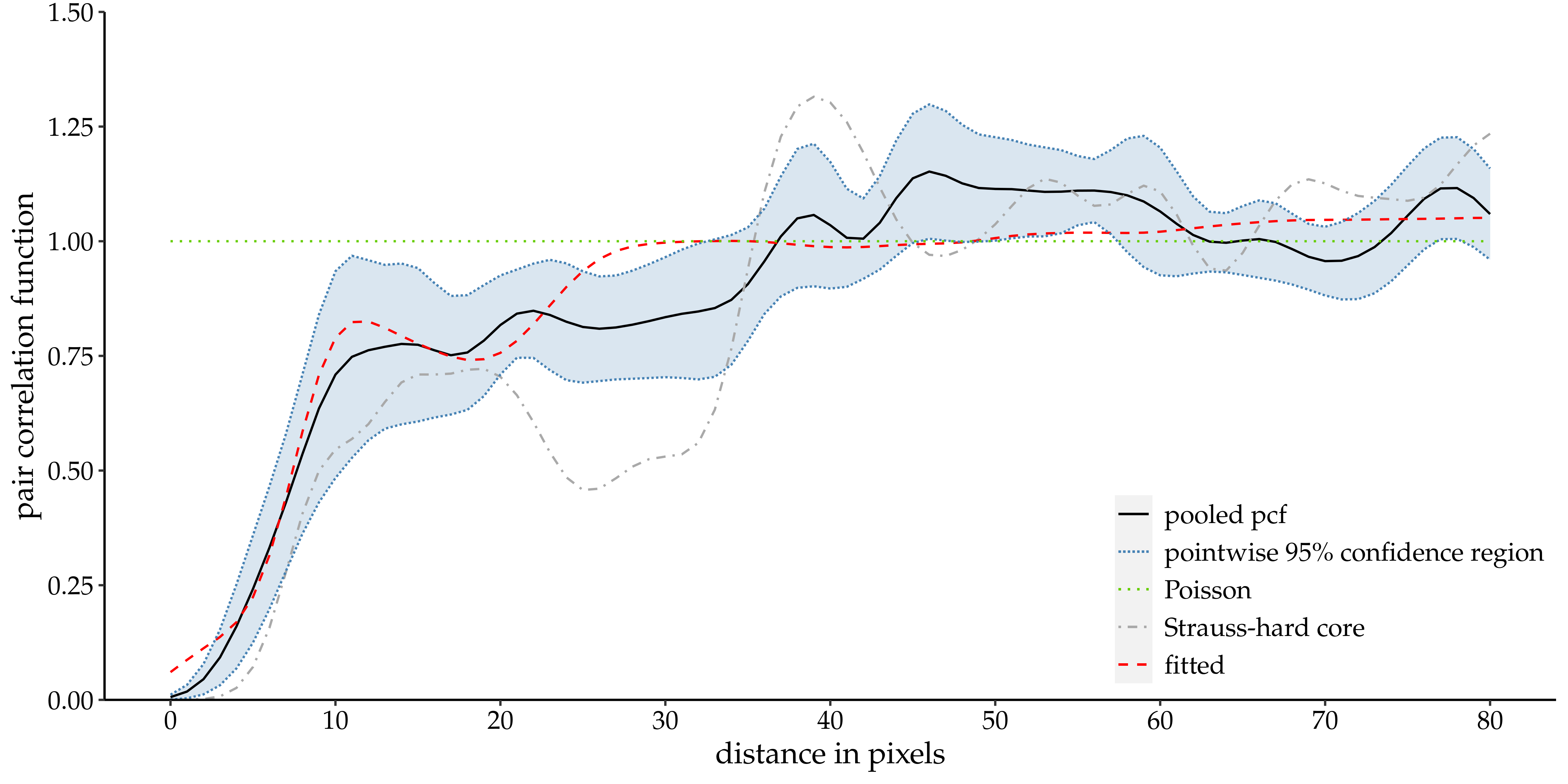
Figure 5 shows roughly two regimes of interaction. A regime of very strong inhibition in the range up to about 5–10 pixels and a regime of moderate inhibition up to 35–40 pixels. This suggests modelling the bulk of the minutiae by a two-scale Strauss process; see [27, Example 6.2]. We choose zero interaction at distances (hard core, banning points closer than ) and interaction at distances , and refer to the resulting point process as a Strauss process with hard core. For comparison, the pooled PCF estimate is shown in Figure 5 (dash-dotted grey curve) based on 20 simulated Strauss processes with hard core, having activity functions , , where is the necessary minutiae intensity (3) obtained from the -th fingerprint image. The hard core distance was chosen as the average inter-ridge distance (see Section 2). A pilot study on FVC2002 DB1 suggested that a Strauss interaction distance of approximately three times the average inter-ridge distance seems to be a reasonable choice since only about 6% of all minutiae pairs of the considered fingerprints have a smaller distance. The parameters and are reasonable choices in view of the simulations considered later in Section 6. Note that the real minutiae patterns also contain the random minutiae, which essentially explains that the grey curve is visibly too small for values up to approximately . To demonstrate that this deficiency will be suitably corrected once we apply our model in Section 6 to the same data, we also show the PCF from that model fit (dashed red curve). Clearly our choice of is somewhat too small, as we will discuss in Section 6.
As a model for the random minutiae process , we choose a homogeneous Poisson process with unknown intensity . Such a process has density
w.r.t. the standard Poisson process (homogeneous Poisson process with intensity ), see [27, Proposition 3.8]. Here denotes the set of all finite point configurations of and is the number of points in . Ignoring that, in practice, random minutiae cannot be closer than the inter-ridge distance is harmless as their intensity is rather low, both in absolute terms and compared to the intensity of necessary minutiae (see Remark 3.1).
If we also assumed that the necessary minutiae process was a Poisson process, but inhomogeneous with intensity proportional to (3), then would also be Poisson distributed, cf. [27, Proposition 3.6]. Under this assumption the theoretical pair correlation function would be one which, with regard to Figure 5, contrasts reality.
Last but not least, modelling the necessary minutiae as a point process with substantial inhibition of points is also advantageous from a conceptual point of view: up to certain errors arising from the discretization of the OF and RF into minutiae information as well as from data acquisition and processing, the necessary minutiae counts should be determined by the underlying necessary minutiae intensity. Some inhibition between points is required to keep the variances of minutiae counts in regions with high necessary minutiae intensity small enough to be compatible with the data. Simulations we performed (not shown here) indicate that inhomogeneous Poisson processes based on the same intensity have much too high variances.
The Strauss process with hard core has density
w.r.t. to the standard Poisson process. Here is the hard core distance,
is the minimum inter-point distance in (by convention shall always exclude the case ) and
is the number of pairs of points that lie within the interaction distance of each other. The activity or trend function governs the intensity and takes up OF divergence and RF divergence and is the repulsion strength at distances , meaning each point pair at distance in is penalized by a factor . Based on formula (3), we assume
| (6) |
for some factor . The factor denotes the normalising constant of the probability density and is intractable, cf. [27, Section 6.2]. We expect that is in fact larger than one because the presence of repulsion requires an activity larger than a Poisson intensity yielding comparable number of observed points, e.g. [17, 13]. Even in the homogeneous case it is not clear, how and interact, [4, 12] give some approximations.
The interaction distances and are assumed to be known in advance, since joint estimation of simultaneously is notoriously difficult due to strong negative correlation, cf. [31]. We choose the hard core distance as the average inter-ridge distance of the finger – which seems to be be fairly realistic – and the interaction distance to be three times as large, see above.
The observed minutiae pattern can then be written as where and are realizations of and , respectively. We introduce a latent variable where , so that means that minutia is necessary. We combine the parameters into a vector . Then, by independence of and , the density of given is given by
| (7) |
The question arises how to find suitable values of and an assignment of the minutiae to and . The computation of a maximum likelihood estimator for the parameters is notoriously difficult due to the intractable normalising constant. A maximum pseudo-likelihood approach for the superimposed processes is studied in [37]. While it is computationally expensive, it does not provide information about . Even more importantly, it is questionable whether there is only one single choice of that fits best. Our view is that there likely are several choices which all fit reasonably well, particularly for . Bearing this in mind, we adopt a Bayesian approach, exploring the posterior distribution of given the minutiae point pattern . Not only does this yield information about the parameter values, it also provides a quantification of the uncertainty of the assignment to the classes of necessary and random minutiae.
5 Bayesian Inference using MCMC
For better readability we do not distinguish between random variables and their realizations when writing “” or “”. Given a minutiae pattern , Bayes’ theorem yields for the posterior distribution
| (8) |
where is the likelihood of our data given parameters and labels as described in (7) and models our prior belief about the parameters and labels. We face a doubly intractable problem because the denominator in (8) is intractable, and in the numerator contains another intractable normalising constant. Ignoring the second factor for the moment, we can eliminate the first intractability by applying a Metropolis–Hastings algorithm, see Algorithm 5.1, which produces samples from the posterior distribution (8). For an overview about MCMC methods see e.g. [8] or [20].
Algorithm 5.1 (Framework for the Minutiae Separation Algorithm (MiSeal)).
| (9) |
Remark 5.2.
The performance of Algorith 5.1 crucially depends on the computation of the Hastings ratio (9). Applying (8), this can be written as
| (10) |
In the following sections we elaborate further details on how to compute the individual quotients, the choice of our priors as well as the update procedures for and .
For the updates, we employ a random scan Gibbs sampler [20] with update probabilities for and for because the computation of the Hastings ratio for a joint update turned out to be difficult. A value of (reflecting on average 19 proposed flips out of the approx. 30–60 minutiae per finger for each update) approximately yields the fastest mixing. The update for each component employs a Markov chain yielding a variant from the Metropolis-within-Gibbs class of algorithms, see [33].
5.1 Choice of priors
We write and assume the prior of the parameters is a product of the priors of the single parameters chosen as follows.
We choose where the parameters are chosen such that the expected value of equals one (see around (6)) and the variance is reasonably large. For flexibility we choose to be beta distributed with , (hence, ), since we expect the process to be rather inhibitive also outside the hard core distance.
For the intensity of the random minutiae we choose the prior to be a Gamma distribution . Being conjugate to the Poisson likelihood, this prior has the advantage that we do not have to perform Hastings steps when updating , but can draw directly from the posterior distribution conditional on and , cf. (12) below. We choose the parameters , such that the expected value of the prior is from (5) and its variance is such that the ratio of standard deviation over mean is reasonably sized.
Furthermore, for every imprint featuring minutiae in its region of interest , Remark 3.1 yields an expected number of random minutiae in . Hence, for each finger individually, we choose the prior for the label vector as with and . We discard infeasible label vectors, i.e. label vectors for which some pairs of have distance smaller than and thereby violate the hard core condition. The ratio of priors for different parameters , thus computes as
| (11) |
where denote the number of ones in , respectively.
We have adjusted the variances of the priors such that they concentrate on a domain we deem reasonable according to a pilot study (not shown here). We keep them rather uninformative, however, to avoid undesirable dependence of the posterior on our particular prior choices.
5.2 Update of
When updating , we randomly choose to update either or . To this end, toss a coin with success probability (this is slightly smaller than , taking into account that, due to the explicitly available posterior, see below, there are no rejects for the -updates). In case of success, update , which, since the Gamma prior is conjugate for the Poisson likelihood, we can draw directly from the posterior distribution, namely from
| (12) |
where is the number of minutiae currently labelled as random in . Note that this does not depend on any of the other parameters of nor on the current state of .
In case of failure, we update the parameters of the Strauss process by proposing a normally distributed step in the natural parameter space (-space), i.e. our proposal is log-normally distributed,
| (13) |
where the parameters , , are fixed (see end of this subsection). Denote the covariance matrix in (13) by . Then, the proposal density for a -update from to is given as
and hence
| (14) |
To compute the Hastings ratio for the -update, we consider the likelihood ratio
| (15) |
Note that this ratio still contains a ratio of normalising constants which cannot be computed explicitly. To overcome this problem, we apply the auxiliary variable method which goes back to [7]. For application in point processes we refer to [6, 24, 31, 30] and the references therein.
To this end, we extend the state space and introduce an auxiliary point pattern with density w.r.t. the standard Poisson process which does not depend on the current . The point pattern is then included in the model as an additional variable. For this, we have to define a new proposal distribution on the extended state space, which we choose as
i.e. we draw the new auxiliary point pattern independently of the current auxiliary point pattern as a realization of a Strauss process with hard core having parameter , whereas the proposal for the parameter remains as before. Then, the Hastings ratio for a parameter update from to is
| (16) |
where the ratio of priors and proposals can be obtained from (11) and (14), respectively. Since the normalising constants of the two -terms and the two -terms cancel, this Hastings ratio can be computed explicitly. However, in every update we have to draw a new point pattern from a Strauss process with hard core, for which we again have to run a Markov chain. This requires a considerable additional effort in each update step for .
A crucial influence on the algorithm’s performance is the choice of which ideally should fit well to the proposal density . The best choice would of course be to choose , which is not feasible since then (16) would contain the normalising constants again. In [31], the density of a Poisson process was used, which results in rather poor mixing behaviour, cf. [31, Figure 6]. We therefore choose for the density of another Strauss process with hard core, fixing its parameter at , where is the current label vector and is the maximum pseudo-likelihood estimate (MPLE) based on the minutiae currently labelled as necessary; see e.g. [5, Section 13.13] and the references given there. If we knew the true in advance, this would be a good initial guess for the parameters. However, in practice the true is not known. We therefore adapt iteratively during burn-in and keep it fixed for the rest of the run, so that we still obtain convergence to the desired posterior distribution.
For the proposed MCMC algorithm the proposal variances , and correlation have to be determined. To this end, we considered for reasonable values of and a pilot sample and estimate the correlation coefficient as its sample correlation. The corresponding proposal variances are then adjusted such that the acceptance rate for a parameter proposal is about which is optimal according to [32]. For our computations we set , and .
5.3 Update of
When updating , we pick one component of uniformly at random, , say, and propose to flip it to , while keeping the other components unchanged, for . Writing for the partition in random and necessary minutiae before and after the proposed flip, respectively, we either have , if the flip of is from to or , if the flip is from to . Thus, the Hastings ratio is given as
| (17) | ||||
Here, denotes the number of -close neighbours of in . Note that in the last equality we used that the first factor of (17) is equal to 1, which is valid after the burn-in phase, when we do not update the parameters of the auxiliary target density anymore. By contrast, it seems that the same factor was erroneously omitted in [31, Section 3.2.2]. It is not equal to there, because the auxiliary target density is homogeneous Poisson with intensity depending on (in our notation). This may be another part of the reason for the unfavourable mixing behaviour in [31].
6 Performance of the Minutiae Separating Algorithm
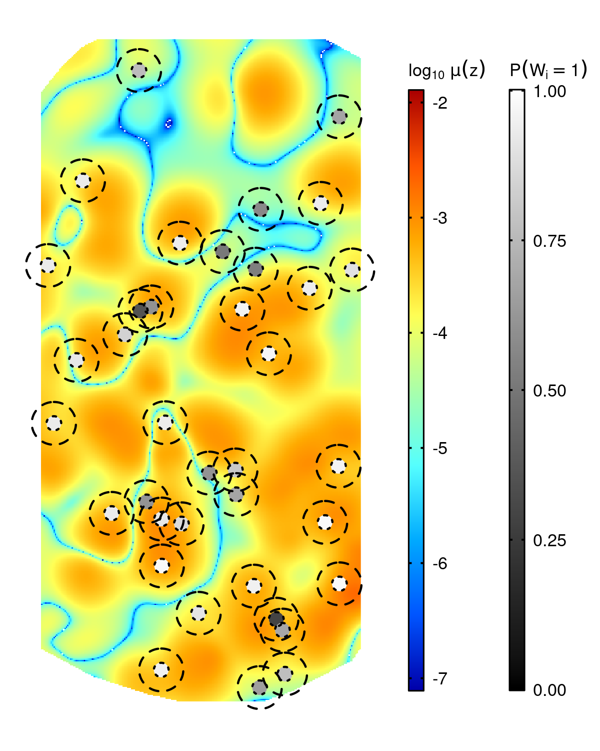
In order to benchmark MiSeal for separating random from necessary minutiae, we first simulate a test scenario close to real fingerprints with true parameters known. To this end, for each of the manually marked 20 fingerprints, we compute a smoothed necessary minutiae intensity function building on from (3), draw “true” parameters from the priors specified in Section 5.1 and simulate a sample of superimposed random and necessary minutiae following the model (7). Such a simulated minutiae pattern is depicted in Figure 6(b); the original minutiae pattern of the same print is seen in Figure 6(a) and the heat map of the necessary minutiae intensity on which the simulation is based in Figure 6(c).



We determine the parameter for the auxiliary point pattern density as follows: During the burn-in phase of iterations, we compute after every iterations the MPLE () for given the current labels and use for the next iterations. We then use the component-wise mean as value for for the rest of the entire run (alternatively, one could take the mean in the natural parameter space). The MPLE can be efficiently computed using the ppm function of the R package spatstat [5].
We then use the samples from the posterior of the parameter as well as the labels . Trace plots and the estimated posterior densities for the Strauss parameters for the example in Figure 6(b) are shown in Figures 6(d), 6(e) and 7. Overall, we observe good mixing behaviour of the Markov chain even though the parameter for the auxiliary variable method was only determined heuristically. In all 20 cases the posterior distributions concentrate around the true parameters, exemplarily shown in Figure 7. In 11 out of 20 cases has been overestimated as in Figure 6(d) and in 12 out 20 cases has been overestimated as in Figure 6(e). This suggests that our method is not substantially biased in one or the other direction. Since the updates are drawn directly from the posterior distribution, we do not show any trace plots but simply remark that estimates concentrate well in the vicinity of the true value.
The univariate marginals of the posterior distribution of the label vector are depicted in panel of Figure 6(c) in grey values ranging from certainly random (black) to certainly necessary (white). While overall the minutiae separation is not too far from the truth, minutiae in regions of large necessary minutiae intensity not violating the Strauss hard core condition are more likely classified as necessary. In contrast, minutiae in regions of low intensity or those lying very close to one another are more likely classified as random.
We finally apply MiSeal to real minutiae patterns of real fingerprints, including the one depicted in Figure 6(a). Again we obtain good mixing behaviour for the parameter estimation. Figure 8 depicts the estimated posterior means for for the 20 considered fingerprints which are rather spread out in the parameter space. This suggests, even though we assume that they have the same interpretation for all fingerprints, that they also depend on unobserved quantities, such as quality and resolution of the image or manner of imprinting on the acquisition medium.
For each of the data fingerprints we numerically approximated the theoretical PCF of the process fitted in terms of the posterior mean based on 100 draws from the model, cf. Figure 8. The resulting PCFs are pooled and also depicted as a red dashed curve in Figure 5. We observe that the PCFs of the fitted processes run mostly within the pointwise confidence band, however it seems clear that the chosen based on a pilot study is somewhat too small. The preselection of the interaction radii and leaves potential for future research. It may be desirable to adjust using more sophisticated characteristics of the individual fingerprint than just the average inter-ridge distance. At small distances, the PCFs tend to be slightly above the confidence band due to Poisson minutiae forming close pairs with other minutiae. This might not be very relevant in practice, and in any case it is hard to avoid this behaviour without making the model mathematically much more difficult. As a final remark, we note that a global way of assessing the model fit might be more desirable. One approach in this direction is given by the global envelope-based goodness-of-fit tests in [26] and [25], which have been developed for a single observation of a point pattern. An extension of the approach provided there to replicated point patterns is beyond the scope of this paper.


Moreover, we observe that the marginal posteriors of are not independent. Considering minutiae pairs within interaction distance from each other, Fisher’s exact test always rejects the hypothesis of independence at the level.
As an example, Table 1 gives the sampled posterior frequencies of the different label pairs for the two minutiae marked on Figure 6(a) with and (halfway north-west from the whorl). In parentheses are the expected frequencies under independence. Notably, we thinned the run by 100 (a little more than the integrated auto-correlation time), resulting in approximately independent subsamples. We partitioned these subsamples in 100 batches and computed batch-wise [23] correlation coefficients to obtain a Monte Carlo estimate of the dependence between and . This yields a correlation of –0.093 on average (with standard error of 0.007), suggesting negative correlation. Moreover, we compute the Kullback-Leibler divergence of the joint distribution of to the closest independent distribution resulting in a Kullback-Leibler divergence of 0.0069 (using base-2 logarithms).
| 0 | 1 | total | |
|---|---|---|---|
| 0 | 73 (172) | 636 (537) | 709 |
| 1 | 2,349 (2,250) | 6,942 (7,041) | 9,291 |
| total | 2,422 | 7,578 | 10,000 |
7 Random Minutiae Are Characteristic
Here we consider the two fingerprints from [28], already shown in Figure 2. At first glance, they appear very similar based on their OFs, but actually stem from two different persons.
As before, we enhance these images and extract the minutiae manually. Then, we approximate the posterior distributions , of the label vectors with our MiSeal (Section 5). Their marginal probabilities are depicted in the right bottom of Figure 9. In particular the north-east part of the right print in Figure 9 contains candidates for random minutiae (from grey to black), that are not found on the left print. Notably, such candidates tend to cluster which indicates their high correlation. In a realization, however, within such a cluster only as many minutiae will be random as the sum of marginal probabilities indicates, so that most clusters disappear (compare also Figure 6(b) with Figure 6(c)), making the random minutiae pattern Poissonian.


For comparison of two minutiae patterns we use the Minutiae Cylinder Code (MCC) matching algorithm obtained from [10], which is publicly available. The MCC compares two given minutiae templates exploiting local information, i.e. spatial and directional similarity of minutiae and their neighbourhood (cylinders) and combines the most similar cylinders to a global score where 1 means very similar and 0 means very different. In order to assess characteristicness of random minutiae, we investigate whether deleting random minutiae leads to more similar fingerprints than deleting the same number of arbitrary minutiae. For this, we repeat the following procedure times:
- (1)
Draw a sample from the posterior of the labels and let be the number of random minutiae in the minutiae template , .
- (2)
Delete from the minutiae template the minutiae labelled as random under to obtain a new template containing only the necessary minutiae, .
- (3)
Draw uniformly at random minutiae from and delete them from to obtain a new template having the same number of minutiae as , .
- (4)
Compute the matching scores and using the MCC.
We then compute the differences between these 1,000 pairs of matching scores. Note that local clusters of minutiae, which make a major contribution to the MCC matching score, are often dissolved by our deletion scheme, leading to scores on a very small scale. We therefore consider the relative score differences in Figure 10. We obtain a Monte Carlo estimate of 93.6% (with standard error of 0.8%) that the matching score after deletion of random minutiae is larger than the score after deleting the same number of minutiae at random. Similarly, the Monte Carlo estimate for the relative difference of scores yields a 23.7% improvement (with standard error of 0.6%).

Hence, we may conclude that the two different fingerprints become more similar to one another after deleting the random minutiae in comparison to just randomly deleting minutiae. This preliminary proof of concept suggests that for fingerprints with similar OFs the information encoded in random minutiae is characteristic to distinguish them from one another.
8 Discussion
We have introduced a model which provides a formula for predicting locally the number of necessary minutiae determined by OF and RF of a fingerprint. In a statistical analysis, based on 20 high quality images, we have found that fingerprints feature additional random minutiae. By considering the pair correlation function for the same data, we have concluded that it is reasonable to model the necessary minutiae by a Strauss process with hard core, while the additional random minutiae can be modelled by a homogeneous Poisson point process.
For the independent superposition of the two processes, we can apply an MCMC algorithm for exploring the distribution of necessary and random minutiae of a given fingerprint as well as, simultaneously, the model parameters. The proposed MiSeal (Section 5) is based on the work of [31] but provides significant improvements in terms of mixing times and does not need assumptions on the independence of the components of the label vector as in [30]. A crucial ingredient for good mixing seems to be a good choice of the marginal distribution for the auxiliary point pattern. The associated parameter also has to be chosen appropriately which we achieve by repeated estimation during the burn-in phase. As a future improvement, updating of can also be performed during the entire run if we let the adjustments diminish and adapt the Hastings ratio for the -update appropriately.
It turned out that, for two similar yet different fingerprints, excluding random minutiae yields a highly significant improvement of the similarity score as compared to excluding arbitrary minutiae. This suggests that the random minutiae carry characteristic information of fingerprint individuality going beyond OFs and RFs, which is why we refer to them as characteristic minutiae.
The extent to which this information can effectively be used for discriminating different fingerprints with similar OFs is the subject of current and future research. One important ingredient will be sufficiently robust minutiae extraction.
Additionally, various parameters of our MiSeal, for instance the smoothing of the necessary minutiae intensity, can be more finely tuned based on larger data sets. Eventually, we expect that including the degree of characteristicness of minutiae will improve error rates of minutiae matching algorithms.
Acknowledgements
Johannes Wieditz gratefully acknowledges support by the DFG Research Training Group 2088 “Discovering structure in complex data: Statistics meets Optimization and Inverse Problems”. The first and the last author further gratefully acknowledge support by the Niedersachsen Vorab of the Volkswagen foundation and the Felix-Bernstein-Institute of Mathematical Statistics in the Biosciences. Yvo Pokern also wishes to thank the Royal Society for International Exchanges grant IE150666. We thank Claudia Redenbach for helpful discussions and for providing the code from [31], [30]. The authors are also grateful to Corvin Grigutsch for writing large parts of the software. In conclusion, we thank the three anonymous referees for their very helpful comments improving the paper.
References
- Adams and Essex [2016] Adams, R. and Essex, C. (2016) Calculus: A Complete Course. Toronto: Pearson Canada, 9th edn.
- Amann and Escher [2008] Amann, H. and Escher, J. (2008) Analysis II. Basel: Birkhäuser, 1st English edn.
- Amann and Escher [2009] — (2009) Analysis III. Basel: Birkhäuser, 1st English edn.
- Baddeley et al. [2012] Baddeley, A., Nair, G. et al. (2012) Fast approximation of the intensity of gibbs point processes. Electronic Journal of Statistics, 6, 1155–1169.
- Baddeley et al. [2015] Baddeley, A., Rubak, E. and Turner, R. (2015) Spatial point patterns: methodology and applications with R. Chapman and Hall/CRC.
- Berthelsen and Møller [2006] Berthelsen, K. K. and Møller, J. (2006) Bayesian analysis of Markov point processes. In Case studies in spatial point process modeling. Springer.
- Besag and Green [1993] Besag, J. and Green, P. J. (1993) Spatial statistics and Bayesian computation. Journal of the Royal Statistical Society: Series B (Methodological), 55, 25–37.
- Brooks et al. [2011] Brooks, S., Gelman, A., Jones, G. and Meng, X.-L. (2011) Handbook of Markov Chain Monte Carlo. CRC press.
- Cameron and Trivedi [2013] Cameron, A. C. and Trivedi, P. K. (2013) Regression analysis of count data, vol. 53. Cambridge university press.
- Cappelli et al. [2010] Cappelli, R., Ferrara, M., Maltoni, D. and Tistarelli, M. (2010) MCC: A baseline algorithm for fingerprint verification in FVC-onGoing. In 2010 11th International Conference on Control Automation Robotics Vision, 19–23.
- Chen and Moon [2006] Chen, J. and Moon, Y.-S. (2006) A statistical study on the fingerprint minutiae distribution. In 2006 IEEE International Conference on Acoustics Speech and Signal Processing Proceedings, vol. 2. IEEE.
- Coeurjolly et al. [2018] Coeurjolly, J.-F., Lavancier, F. et al. (2018) Intensity approximation for pairwise interaction gibbs point processes using determinantal point processes. Electronic journal of statistics, 12, 3181–3203.
- Eckel et al. [2009] Eckel, S., Fleischer, F., Grabarnik, P., Kazda, M., Särkkä, A. and Schmidt, V. (2009) Modelling tree roots in mixed forest stands by inhomogeneous marked gibbs point processes. Biometrical Journal: Journal of Mathematical Methods in Biosciences, 51, 522–539.
- Gottschlich and Huckemann [2014] Gottschlich, C. and Huckemann, S. (2014) Separating the real from the synthetic: minutiae histograms as fingerprints of fingerprints. IET Biometrics, 3, 291–301.
- Hong et al. [1998] Hong, L., Wan, Y. and Jain, A. (1998) Fingerprint image enhancement: algorithm and performance evaluation. IEEE transactions on pattern analysis and machine intelligence, 20, 777–789.
- Huckemann et al. [2008] Huckemann, S., Hotz, T. and Munk, A. (2008) Global models for the orientation field of fingerprints: an approach based on quadratic differentials. IEEE Transactions on Pattern Analysis and Machine Intelligence, 30, 1507–1519.
- Jensen and Nielsen [2001] Jensen, E. B. V. and Nielsen, L. S. (2001) A review on inhomogeneous markov point processes. Lecture Notes-Monograph Series, 297–318.
- Kücken and Champod [2012] Kücken, M. and Champod, C. (2012) Merkel cells and the individuality of friction ridge skin. Journal of Theoretical Biology.
- Kücken and Newell [2007] Kücken, M. and Newell, A. (2007) A model for fingerprint formation. EPL (Europhysics Letters), 68, 141.
- Liu [2004] Liu, J. S. (2004) Monte Carlo Strategies in Scientific Computing. Springer.
- Maio et al. [2002] Maio, D., Maltoni, D., Cappelli, R., Wayman, J. L. and Jain, A. K. (2002) FVC2002: Second fingerprint verification competition. In Object recognition supported by user interaction for service robots, vol. 3, 811–814. IEEE.
- Maltoni et al. [2009] Maltoni, D., Maio, D., Jain, A. K. and Prabhakar, S. (2009) Handbook of fingerprint recognition. Springer Science & Business Media.
- Matthews [1975] Matthews, B. W. (1975) Comparison of the predicted and observed secondary structure of t4 phage lysozyme. Biochimica et Biophysica Acta (BBA)-Protein Structure, 405, 442–451.
- Murray et al. [2012] Murray, I., Ghahramani, Z. and MacKay, D. (2012) MCMC for doubly-intractable distributions. arXiv preprint arXiv:1206.6848.
- Myllymäki and Mrkvička [2019] Myllymäki, M. and Mrkvička, T. (2019) GET: Global envelopes in R. arXiv preprint arXiv:1911.06583.
- Myllymäki et al. [2017] Myllymäki, M., Mrkvicka, T., Grabarnik, P., Seijo, H. and Hahn, U. (2017) Global envelope tests for spatial processes. Journal of the Royal Statistical Society.
- Møller and Waagepetersen [2003] Møller, J. and Waagepetersen, R. P. (2003) Statistical inference and simulation for spatial point processes. Chapman and Hall/CRC.
- Newman [1930] Newman, H. H. (1930) The finger prints of twins. Journal of Genetics, 23, 415–446.
- Nikodémusz-Székely and Székely [1993] Nikodémusz-Székely, É. and Székely, V. (1993) Image recognition problems of fingerprint identification. Microprocessors and Microsystems, 17, 215–218.
- Rajala et al. [2016] Rajala, T., Redenbach, C., Särkkä, A. and Sormani, M. (2016) Variational Bayes approach for classification of points in superpositions of point processes. Spatial Statistics, 15, 85–99.
- Redenbach et al. [2015] Redenbach, C., Särkkä, A. and Sormani, M. (2015) Classification of points in superpositions of Strauss and Poisson processes. Spatial Statistics, 12, 81–95.
- Roberts et al. [1997] Roberts, G. O., Gelman, A. and Gilks, W. R. (1997) Weak convergence and optimal scaling of random walk Metropolis algorithms. The Annals of Applied Probability, 7, 110–120.
- Roberts and Rosenthal [2006] Roberts, G. O. and Rosenthal, J. S. (2006) Harris recurrence of metropolis-within-gibbs and trans-dimensional markov chains. The Annals of Applied Probability, 2123–2139.
- Stoney [1988] Stoney, D. A. (1988) Distribution of epidermal ridge minutiae. American Journal of Physical Anthropology, 77, 367–376.
- Thai et al. [2016] Thai, D. H., Huckemann, S. and Gottschlich, C. (2016) Filter design and performance evaluation for fingerprint image segmentation. PloS One, 11.
- Wieditz [2020] Wieditz, J. (2020) Minutiae Separating Algorithm (MiSeal). https://github.com/jwieditz/MiSeal.
- Wieditz et al. [2021] Wieditz, J., Pokern, Y., Schuhmacher, D. and Huckemann, S. (2021) Maximum pseudo-likelihood parameter estimation in superpositions of Strauss and Poisson processes (manuscript).