Multilayered density profile for noninteracting fermions in a rotating two-dimensional trap
Abstract
We compute exactly the average spatial density for spinless noninteracting fermions in a harmonic trap rotating with a constant frequency in the presence of an additional repulsive central potential . We find that, in the large limit, the bulk density has a rich and nontrivial profile – with a hole at the center of the trap and surrounded by a multi-layered “wedding cake” structure. The number of layers depends on and on the two parameters and leading to a rich phase diagram. Zooming in on the edge of the layer, we find that the edge density profile exhibits kinks located at the zeroes of the Hermite polynomial. Interestingly, in the large limit, we show that the edge density profile approaches a limiting form, which resembles the shape of a propagating front, found in the unitary evolution of certain quantum spin chains. We also study how a newly formed droplet grows in size on top of the last layer as one changes the parameters.
I Introduction
Noninteracting spinless fermions in a confining trap is a subject of much current theoretical and experimental interest Bloch et al. 2008; Nascimbene et al. 2010; Cheuk et al. 2015; Haller et al. 2015; Parsons et al. 2015; Mukherjee et al. 2017; Hueck et al. 2018. On one hand, this system is realisable in cold atom experiments, and several techniques such as absorption imaging Inguscio et al. 2008; Giorgini et al. 2008; Joseph et al. 2011 for collective density measurements and quantum gas microscopes Cheuk et al. 2015; Haller et al. 2015; Parsons et al. 2015 for direct in situ imaging of the individual fermions with remarkably high resolutions are available. On the other hand, it is simple enough to be analytically tractable and yet exhibits rich and nontrivial spatial fluctuations, even at zero temperature, due to the Pauli exclusion principle Vicari 2012; Eisler 2013; Marino et al. 2014; Dean et al. 2015; Dean et al. 2015; Dean et al. 2016; Marino et al. 2016. While the bulk density is usually well described by the local density approximation (LDA) Butts and Rokhsar 1997; Inguscio et al. 2008, this approximation breaks down near the edges of the Fermi gas, induced by the trap. A number of recent studies have pointed out that LDA is not sufficient to capture the density fluctuations and correlations near the edges Kohn and Mattsson 1998; Eisler 2013; Dean et al. 2015; Dean et al. 2015; Dean et al. 2016. For certain one-dimensional trapping potentials, such as the harmonic trap, an exact mapping was found between the positions of the fermions in the ground state and the eigenvalues of a suitable random matrix ensemble Eisler 2013; Marino et al. 2014 – for a recent review see Dean et al. 2019. Using results from the random matrix theory (RMT), the density correlations near the edges were computed exactly and their universal properties (with respect to the shape of the trapping potential) were elucidated Eisler 2013; Dean et al. 2015; Dean et al. 2015; Calabrese et al. 2015; Dean et al. 2016; Lacroix-A-Chez-Toine et al. 2017; Dean et al. 2018; Le Doussal et al. 2018; Cunden et al. 2019. The connection to RMT does not hold generically in higher dimensions. However, using the determinantal properties of the noninteracting fermions, the edge properties in higher dimensions could still be computed analytically Dean et al. 2015; Dean et al. 2016.
A particularly interesting situation corresponds to fermions in a rotating trap in two-dimensions, which has been studied recently both experimentally Ho and Ciobanu 2000; Aftalion et al. 2005; Schweikhard et al. 2004 and theoretically Fetter 2009; Cooper 2008; Lacroix-A-Chez-Toine et al. 2019. In this system, the single particle Hamiltonian, in the rotating frame, is given by Landau et al. 1980; Leggett et al. 2006
| (1) |
where is a confining central potential, is the -component of the angular momentum and is the rotation frequency. For the harmonic trap , an important parameter is the ratio , which must satisfy to keep the fermions confined. The limit corresponds to fermions in a non-rotating harmonic trap while in the opposite limit , this problem can be mapped to the celebrated Landau problem of noninteracting fermions in a plane in the presence of a perpendicular magnetic field Cooper 2012. Interestingly, in this limit, the positions of fermions in the ground state map onto the eigenvalues of the classical complex Ginibre ensemble of RMT Lacroix-A-Chez-Toine et al. 2019, where one considers a random matrix with independent complex Gaussian entries Forrester 2010. In this mapping, one assumes that the fermions are confined in the lowest Landau level, which can be realized by setting . With this assumption, the bulk density for large is rather simple: it is just uniform over the disk of radius centred at the origin Lacroix-A-Chez-Toine et al. 2019.
a)
b) 
c)
This uniform bulk density emerges because, in the ground state, the fermions are all in the lowest Landau level. A natural question then is: how the density may change if the many-body ground state also contains single-particle states belonging to higher Landau levels? Indeed, this is a generic situation as one increases , for fixed . In addition, since the potential is radially symmetric, it is convenient to solve the corresponding Schrödinger equation in polar coordinates, which will automatically generate an effective repulsive interaction in the radial direction. Hence it is natural to consider a more generic potential from the start
| (2) |
We thus have two parameters and . In this paper we investigate the density profile in the ground state, for large , as a function of and and find an extremely rich phase diagram in the plane.
Let us first summarise our main results. We find that in the large limit the appropriate rescaled parameters are
| (3) |
which are both kept of order as . We will show later that this scaling is necessary to keep the average density of fermions of order as . The phase diagram in the plane is depicted in Fig. 1 a). There are series of critical lines that separate the regions labelled by where is the number of Landau levels included in the ground state. As one crosses these critical lines, the density profile undergoes abrupt changes, as shown in Fig. 1 a). For a given the bulk density vanishes for thus creating a hole around the origin [see Fig. 1 b)]. Outside the hole, the density is nonzero over an annulus . On top of this annulus, there is a “wedding cake” structure [see Fig. 1 b)] with layers with progressively smaller supports but with equal heights . For example the -th layer has support on (see Fig. 1). As shown later, . We also investigated the change in the density profile as one crosses the critical lines in the phase diagram and found an interesting “travelling front structure” in the density. Furthermore, if we zoom in on the left boundary of the -th layer (and symmetrically on the right boundary), i.e., close to (and symmetrically at ) we find a nontrivial edge-profile of the density (11) with kinks whose locations coincide with the zeros of the -th Hermite polynomial with denoting the scaled distance from (see inset of Fig. 1 (c)). Finally, in the limit where , the edge profile approaches a nontrivial limiting form, which we compute exactly. Interestingly, the same limiting form has appeared in completely different problems, such as in a propagating one-dimensional fermionic front separating a high and low density phases and evolving unitarily in time Antal et al. 1999; Antal et al. 2008; Eisler and Rácz 2013; Hunyadi et al. 2004; Mukherjee et al. 2018.
II Model and Properties
We start with the single particle Hamiltonian in (1) with in Eq. (2). The model turns out to be integrable in the sense that the Schrödinger equation is exactly solvable in the polar coordinates (see Appendix A for details). For convenience, we set . We get
| (4) |
where are the generalised Laguerre polynomials and the normalisation gives . The associated eigenvalues, in units of , are given by (see Appendix B for details)
| (5) |
The single particle states are labelled by a pair of integers with and . The energy levels (5) are shown in Fig. 2. Different values of correspond to different bands or Landau levels.
We now consider spinless noninteracting fermions in their ground state. The many-body ground-state is thus given by a Slater determinant constructed from single particle eigenfunctions associated to the lowest eigenvalues. For a given , the eigenfunctions participating in the Slater determinant may belong to multiple bands of the spectrum in Fig. 2 with denoting the label of the highest band which is at least partially filled. We also denote by the Fermi energy, i.e. the energy of the highest occupied single particle energy level. The Fermi energy can be tuned by varying . As increases, one sees from Fig. 2, where is indicated by a horizontal line, that more and more states with energy levels below contribute to the ground state since also increases.
The average number density, normalised to , at a point is given by where denotes the expectation value in the ground state. For noninteracting fermions, it can be computed explicitly in terms of single particle eigenfunctions
| (6) |
where denotes the density from the band and is given by
| (7) |

Here, are the locations where the Fermi level intersects the band, i.e. . Solving this equation using (5) (shifting energy by 1, effectively absorbing it in ) gives
| (8) |
For a given , (Eq. 5) has a minimum at where . Note that is independent of and the energy of the band at this minimum is given by . If the Fermi level has to intersect at least one band, we must have which implies . For a fixed , the number of bands below can be obtained by simultaneously requiring and which yields where denotes the integer part of (see Appendix B for details). The relation between the Fermi energy and can be obtained by counting the total number of single particle levels with energy below . This gives which fixes in terms of (see Appendix B for details). For large , it turns out that . So far, the results are exact for arbitrary , and . To make further progress we now work in the large limit and re-scale the two parameters and as in Eq. (3). Thus and are the new rescaled parameters. It turns out that this scaling is necessary to keep for large . In terms of and , we have from Eq. (8), where and .
III Critical lines in the plane
The plane is divided into different regions labeled by separated by critical lines [see Fig. 1 a)]. For there to be bands, we require, . Setting the upper bound, , one gets (see Appendix C for details). Solving this equation for as a function of gives the critical line . Thus, in the plane, we get different regions labeled by . The region between and corresponds to the region with , i.e. the Fermi level includes bands below it. For instance, and can be explicitly computed (see Appendix C for details) and are plotted in Fig. 1 a), e.g., where is the Heaviside step function.
IV Density in the large-N limit
We start by analysing the large limit of in Eq. (7) upon setting . Since , we can replace the discrete sum over by an integral. We show (see Appendix D and E for details) that it converges to the following form
| (9) |
where and is the Hermite polynomial. For fixed , as , the two bounds and iff . If is outside this interval, both bounds tend to either or simultaneously. In the latter cases, the integral in (9) vanishes as . In contrast, in the former case, the integral approaches a finite value . Hence we conclude that the density from the band at a fixed rescaled distance converges to
| (10) |
where the function takes value if the inequality in the subscript is satisfied and otherwise. Thus the bulk density is flat (with value ) inside the annulus [see Fig. 1 b)]. We find in Fig. 1 c) an excellent agreement between the results obtained from the exact evaluation of the sum in (6) and (7) for and the large bulk density in Eq. (10). For a fixed , the sum in Eq. (6) gives a superposition of contributions of the type (10) for each , leading to the “wedding cake” structure in Fig. 1 b).
If is close to one of the two edges, say the left edge , we can estimate the limiting form of the edge density when from the same Eq. (9). For this, we set where . In this case, the lower limit in the integral in Eq. (9) becomes (with measuring the scaled distance from the left edge), while the upper limit still approaches to as . Hence, we get,
| (11) |
where . Note that when , , and the edge density matches smoothly with the bulk density. In Fig. 1 we have zoomed in on the left edge of layer and plotted the scaling function in the inset, which clearly shows a kink where . For the layer, setting (which implies ), it follows that there will be kinks in whose locations coincide with the zeros of . The scaling function is actually universal in the sense that it does not depend on and explicitly. In fact, in the special case and , but with fixed (the classical Landau problem) – hence not in the scaling limit discussed here –, the edge density for the Landau level was studied in Dunne 1994 and similar kinks were found for finite , but the scaling function was not computed (see also Haimi and Hedenmalm 2013 in the mathematics literature in the context of polyanalytic Ginibre ensembles).
Furthermore, an interesting limiting shape emerges for in the scaling limit of large and large but with the ratio fixed. In this case, we find (see Appendix E for details)
| (12) |
and for it takes a value of . Interestingly, a similar shape appeared in the description of a propagating front in the quantum evolution of a spin chain (equivalent to free fermions on a lattice) Antal et al. 1999; Antal et al. 2008; Eisler and Rácz 2013; Hunyadi et al. 2004; Mukherjee et al. 2018. It turns out that there is yet another interesting scaling regime close to the two endpoints . For example, setting with
| (13) |
where where denotes the Airy function. Interestingly, the same scaling function describes the tail of the density of eigenvalues (centered and scaled) in the Gaussian Unitary Ensemble of RMT Bowick and Brézin 1991; Forrester 1993.

V Crossing the critical line in the plane
When changes from to (which means a new band is included below the Fermi level), one may wonder how the density profile changes from a one-layered structure to a two-layered structure. When one crosses this critical line , the second layer appears on top of the first layer (Fig. 1). Here, we describe the evolution of the density profile of this newly formed droplet as a function of the distance below the critical line for fixed (see Appendix F for details). As changes from to , the Fermi level exceeds the value by a small amount : where . As jumps from to , we find that the additional macroscopic density in the second layer appears over the scaled region where and . Therefore, the center of the second layer appears at . Here, we give a scaling description of this density in the second layer just after its appearance, i.e., in the limit . Let , where measures the distance from the center of the second layer. We analyse Eq. (7) with by replacing, for large , the sum by an integral and evaluating it by the saddle point method (see Appendix F for details). This leads to the following density profile of the droplet (for a plot see Fig. 3)
| (14) |
where with being the complementary error function. Here is the scaled distance measured from the center of the droplet, while is proportional to , measuring the deviation from the critical line. If we interpret and as space and time, the density profile in Eq. (14) has an interesting interpretation: the two edges of this profile move ballistically away from the droplet center with a constant speed . At large , the widths of these “solitonic” fronts remain of while the height of the density behind the fronts approaches a constant value (see Fig. 3). This picture can be easily generalized to other critical lines in the plane (see Appendix F for details).
VI Conclusions
To conclude, we have shown analytically that the average density profile in the ground-state of noninteracting fermions in a rotating trap exhibits a rich multi-layered “wedding cake” structure, as more and more Landau levels participate in the ground state by increasing , leading to a highly interesting phase diagram in the parameter space. This non-trivial density profile owes its origin entirely to quantum effects, and can not be obtained from a simple Local Density/Thomas-Fermi approximation. It would be interesting to study the effect of the inclusion of more and more Landau levels on other observables, going beyond the one-point function studied in this paper, such as the number variance and the entanglement entropy (see for e.g., Lacroix-A-Chez-Toine et al. 2019; Rodríguez and Sierra 2009; Charles and Estienne 2019; Leschke et al. 2020). We note that strongly interacting bosons and fermions have been studied experimentally in rotating traps leading in particular to the formation of vortex lattices rotate_cornell; rotate_zwierlein. In our case, there is a hole in the density at the center of the trap, but this is due to the repulsive inverse square interaction and it is not related to a vortex. It will be challenging to see how interactions can change the above scenario, in particular leading to the generation of vortices.
Acknowledgements.
We thank Gautam Mandal and Takeshi Morita for very useful discussions at the initial stage of this work. MK acknowledges support from the project 6004-1 of the Indo-French Centre for the Promotion of Advanced Research (IFCPAR), Ramanujan Fellowship (SB/S2/RJN-114/2016), SERB Early Career Research Award (ECR/2018/002085) and SERB Matrics Grant (MTR/2019/001101) from the Science and Engineering Research Board (SERB), Department of Science and Technology, Government of India. MK thanks the hospitality of Laboratoire de Physique, Ecole Normale Supérieure (Paris). This research was supported by ANR grant ANR-17-CE30-0027-01 RaMaTraF. MK acknowledges support of the Department of Atomic Energy, Government of India, under project no. RTI4001.Appendix A Model and basic properties
As mentioned in the main text, our starting Hamiltonian is,
| (15) |
where is the -component of the angular momentum, characterises the repulsive-like potential at the centre (inverse-square type), is the trap frequency and is frequency at which the trap rotates around the vertical axis. For convenience, we have set the mass and also . Throughout the work, we will consider the case in which the inverse square central potential is very large, i.e.,
| (16) |
In polar coordinates (), the Hamiltonian reads,
| (17) |
where
| (18) |
The first goal is to find eigenstates and eigenvalues of Eq. 17. Let us substitute,
| (19) |
where are integers because the wave function needs to respect periodicity in the angular direction. Then, we get,
| (20) |
Hence, the equation we need to solve is, which gives us,
| (21) |
To reduce the above eigenvalue equation (Eq. 21) to a standard form, we make the following transformation
| (22) |
It is then easy to see that satisfies the differential equation
| (23) |
| (24) |
This is a standard confluent hypergeometric differential equation whose general solution is given by the linear combination of two independent solutions as follows gradshteyn2014table
where and are two arbitrary constants and
is the Kummer’s confluent hypergeometric function. Here, are Pochhammer symbols, i.e., where is a Gamma function. Note that the arguments of the two functions in (A) are different. The function has the following asymptotic behaviors
| (27) |
Hence the most general solution for the eigenfunction in Eq. 22 reads
| (28) | |||||
where and are given in Eq. 24.
To fix these unknown constants and , we first consider the behavior of as . Using Eq. 27 we see that, as , . However, the eigenfunction must be square-integrable, i.e., should be finite. Substituting the small behavior, we see that the integral behaves as in the lower limit . Hence, since , the integral is divergent for all . And this is indeed the case in our problem where is scaled as where and (see Eq. 16). Hence we must have . Therefore the solution now reads
| (29) |
We now consider the other limit . Substituting the asymptotic behaviour given in Eq. 27 in Eq. 29, we find that
| (30) |
Clearly, the integral diverges at the upper limit , provided is finite. Hence, to cure this divergence, we must choose , which means that where is a non-negative integer. In fact, this is the quantisation condition. In fact, when the function is a polynomial of degree and the wave function is square integrable. The quantisation condition , using Eq. 24, reads
| (31) |
The normalization condition fixes the constant , which depends on both quantum numbers and . Hence, summarising, the complete set of eigenfunctions are given by
| (32) |
where with the associated eigenvalues from Eq. 31
| (33) |
Without loss of generality, we will set (i.e., the energies are expressed in units of ) and introduce . Note also that Kummer’s confluent hypergeometric function are related to generalized Laguerre polynomials as,
| (34) |
Therefore, expressing Eq. 32 in terms of generalized Laguerre polynomials is preferable since these functions have an orthonormality condition that turns out to be useful
| (35) |
The normalisation requirement finally gives,
| (36) |
with
| (37) |
Appendix B Analysis of energy levels and the ground state


In this section, we will analyse the energy levels (Eq. 33) and discuss the ground state for a system which has fermions. To start with, let us recap the case.
B.1 case
For , Eq. 15 reduces to the Hamiltonian considered in Refs. Ho and Ciobanu 2000; Aftalion et al. 2005; Lacroix-A-Chez-Toine et al. 2019. The corresponding eigenfunctions were computed not in the polar coordinates, rather in the coordinates where . In this representation, the eigenfunctions read (see e.g. Refs. Ho and Ciobanu 2000; Aftalion et al. 2005; Rodríguez and Sierra 2009; Lacroix-A-Chez-Toine et al. 2019)
| (39) |
with the associated eigenvalues (in units such that )
| (40) |
where and similarly where . This last condition follows from the fact that for , the system is “unstable” in the sense that the fermions can “fly away”. Another important point one can observe is that if , then it becomes the Landau problem (free electrons in perpendicular magnetic field) with energy levels given by,
| (41) |
The lowest Landau level (LLL) is given by . For a given , there is a fold degeneracy. We do not want degeneracy and therefore it can be lifted by choosing . This problem can also be alternatively solved in the polar coordinates discussed in the previous section. To see the connection between these two representations, we put in Eq. 33 and get
| (42) |
where, and . Comparing Eq. 42 and Eq. 40, we get,
| (43) |
which implies,
| (44) |
Therefore the LLL and corresponds to , Note that, when , we have two branches (positive and negative ),
| (45) |
thus the LLL ( and ) corresponds to the right branch () and in the polar representation of the eigenfunctions. The left panel of Fig. 5 shows the energy levels for the case of .
B.2 case assuming where
Now, we discuss the case with . This case turns out to be quite non-trivial. We recap that the energy levels are given by (Eq. 33),
Note that is independent of and the energy of the band at this minimum is given by,
| (48) |
We fix the Fermi level at . By varying , we can intersect the energy spectrum at different points. As increases, more and more -bands of the spectrum become lower than the Fermi level and hence should be included in the construction of the many-body ground-state. The right panel of Fig. 5 shows the energy levels for the case of . It intersects the band at two points along the -axis which can be easily computed by setting and we get,
| (49) |
Note that if the Fermi surface has to intersect at least one band, we must have which indicates that,
| (50) |
For a fixed , the number of bands below can be obtained by setting,
| (51) |
Hence is given by,
| (52) |
where denotes the integer part of . Finally, the relation between the Fermi energy and can be obtained by counting the total number of single particle levels with energy below . This gives,
| (53) |
Using Eq. 49, this gives,
| (54) |
It is important to note that all the above results until now are valid for arbitrary , arbitrary parameters and .
We will now work in the large limit, and set,
| (55) |
Note that we are taking the limit , , keeping fixed. Therefore we have just two parameters and left and we want to calculate the average density in the ground state in the limit of large , for fixed and . We will see that in the plane, there is a series of critical lines separating phases with different density profiles. In terms of and we thus have
| (56) |
where
| (57) |
Appendix C plane and critical lines
The plane gets divided in different regions, each labeled by . For example, if (only the first band is included in the ground state), we must have
| (59) |
The upper inequality gets violated when . Substituting this value of in Eq. 58 with , we get the first critical line in the plane [see Fig. 6],
| (60) |
Hence if , the ground state contains only the band (i.e. ).
Next, let us consider the case , i.e. two bands and are below the Fermi level . From the equation for in Eq. 56 we see that implies
| (61) |
The lower limit corresponds to the critical line discussed before. The upper limit gives a new critical line obtained by substituting in Eq. 58 with , i.e.,
| (62) |
Solving for we get,
| (63) |
This second critical line (Eq. 63) is also plotted in Fig. 6. For higher values of , one can obtain a similar formula for the critical line. For general , the condition indicates that,
| (64) |
Setting in Eq. 58 and simplifying, one gets,
| (65) |
Solving this equation for as a function of gives the critical line . For and the explicit solutions are given respectively in Eqs. 60 and 63. However, one can easily work out the asymptotics. For example the line starts from . For and , this gives and respectively. For large , it is easy to show from Eq. 65 that,
| (66) |
Thus in the plane, we get different regions labeled by . The region between and corresponds to the region with , i.e., the Fermi level has exactly bands below it. In Fig. 6, we show the plane and some critical lines that demarcates various regions. In each region, we have also sketched a typical/representative density profile. Next, we will discuss the density in the ground state.
Appendix D Density as a function of space (exact expression for finite )
We recap (Eq. 36) that the single particle wave functions can be written as
Appendix E Density as a function of space in the large limit
In the large limit, noting that both scale as , we set and replace the discrete sum over by an integral over . Furthermore, we scale . With this change of variable, we want to first express the integrand as a function of for fixed in the limit of large . Let us start with the quantity . Recollecting that and setting , we get for large ,
| (71) |
Approximating the Gamma function in Eq. 70 by the Stirling formula for large and setting , we find to leading order for large ,
| (72) |
where has been defined in Eq. 56. In the large limit, the integral over is dominated by a saddle point at . Therefore it is natural to make the change of variable,
| (73) |
Therefore . We can now use the following remarkable limiting formula for the generalized Laguerre polynomials,
| (74) |
where is the Hermite polynomial of index . Substituting and using we find, using Eq. 74, that,
Thus the integral in Eq. 72 reads
| (76) |
where
| (77) |
Therefore, the density in the band is supported on the interval . It turns out that this expression for the density has very interesting bulk and edge properties. In the subsequent subsections we analyse these properties.
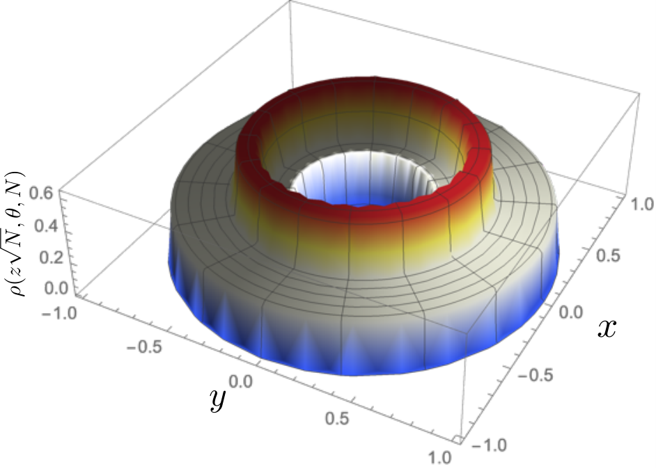
E.1 Bulk
If is in the bulk, i.e. far away from these two edges, then in the large limit, the two limits . Hence the integral becomes simply . This gives the bulk density,
| (78) |
where is an indicator function that takes value if the inequality in the subscript is satisfied and otherwise.
Let us summarise the results of above Sec E.1. The total density is obtained by summing over all the bands below the Fermi energy and is given by its large scaling form,
| (79) |
where the scaling function is given by,
| (80) |
and is given in Eq. 56. One can check that in Eq. 80 is normalized, i.e. upon using the definition of from Eq. 56 and the relation in Eq. 58.
Hence the limiting density has a compact single support over . For , it is just a simple flat density over this support. However, for , the density has a nontrivial layered shape. For example, for , the density is given by (see Fig. 7),
| (81) |
E.2 Edges
In contrast if is close to one of the two edges, say the left edge , we can estimate the limiting form of the edge density when from the same expression in Eq. 76. For this, we set,
| (82) |
where . In this case, the lower limit in the integral in Eq. 76 becomes (with measuring the scaled distance from the left edge), while the upper limit still approaches to as . Hence we get,
| (83) |
where
and we recall that,
| (85) |
Note that when , , and the edge density matches smoothly with the bulk density.
In Fig. 8 we have plotted the edge density functions vs for and . One sees from these figures that the scaling functions have kinks. For , there is only one kink at while for there are two kinks. In general, for the band, the function will have kinks as a function of . The kinks occur when the derivative vanishes, i.e., . By taking the derivative of Eq. 83, we see that this happens when . Thus the locations of the kinks in the edge density of the band coincide with the zeroes of the Hermite polynomial. For instance, for , the kinks are located at and . Note that the edge scaling function is actually universal, i.e. independent of the system parameters and and depends only on the band label . The above non-trivial connection between and Hermite polynomials naturally points to a possible connection to RMT, which we elucidate below.
E.3 Edge density in the limit of high Landau levels () and connection to Random Matrix Theory

It turns out that as , the edge profile given in Eq. 83, property shifted and scaled, has a nice limiting profile. This behaviour comes from the asymptotic behavior of the Hermite polynomials in the limit of large (known as Plancherel-Rotach asymptotics). To obtain this limiting profile, we first set , with , and also perform the change of variable in Eq. 83, . This leads to,
| (86) |
We can now use the Plancherel-Rotach asymptotic formula for Hermite polynomials,
with
Inserting this expansion (Eq. E.3 and Eq. E.3) with in Eq. 86, one finds,
where the indicator function comes from the fact that the asymptotic behavior in Eq. E.3 and Eq. E.3 holds only for , while it is sub-leading (in ) for outside the region. Due to the identity , one can replace , given in Eq. E.3, in the integral over in Eq. E.3 by (the remaining cosine being highly oscillating for large and thus subleading). Therefore we get,
which finally yields (see also Fig. 9),
| (91) |
Close to there is an interesting edge region, of width where the density is described by Airy functions, very similar to the well known “Tracy-Widom” regime at the edge of the Wigner semi-circle in RMT belonging to the Gaussian Unitary Ensemble (GUE). This is somehow expected given the square-root singularity near the edges of the limiting profile given in Eq. 91. This edge behavior can be derived from Eq. 83 by using the asymptotic behavior of the Hermite polynomial near where the Hermite polynomial becomes an Airy function. One finds (for large ), setting with
| (92) |
where
and denotes the standard Airy function. Note that a similar computation could be carried out for the kernel which would lead (on the real line at least) to the well known Airy kernel.
Appendix F Emergence of new droplet as one crosses critical lines in plane
We want to look at the phase diagram in the plane and ask, when changes from to (which means a new band is included below the Fermi energy), how does the density profile change from one layered structure to two layered structure. We have already seen that just when one crosses this critical line , the second layer appears on top of the first layer. In this subsection, we describe the density profile of this emerging blob in the second layer for slightly below for fixed (see Fig. 6), where is given in Eq. 60. We therefore set
| (94) |
For each point in the plane, is uniquely determined from Eq. 58. Therefore as we change the value of from to , the value of also changes from to
| (95) |
where . Inserting this value of in Eq. 58 and expanding for small gives a relation between and
| (96) |
Therefore, one just has one single control parameter describing the location of the system in the phase diagram, in the vicinity of the critical line . We now want to see how the density changes as we vary .
We start with the formula for the density in Eq. 69. When increases from to , the additional density in the second layer is given by,
with
| (98) |
where,
| (99) |
We can rewrite Eq. 99 using Eq. 95 (to leading order in for small ) as,
| (100) |
with
| (101) |
In real space, the second layer of the macroscopic density appears over the scaled region,
| (102) |
where . Therefore, the center of the second layer is located at and we want to provide a scaling description of this density in the second layer just after its appearance, i.e., in the limit . Hence we set,
| (103) |
where is proportional to the distance from the center of the second layer. Thus the density is just a function of and in the vicinity of the critical line and below we work out the dependence of the density on these two parameters in the large limit.
To analyse the density Eq. F in the limit of large , we set and we introduce so that the sum over can be replaced by an integral over leading to,
where we kept the leading term in the arguments for large . We can now approximate the Gamma function by the Stirling’s formula, leading to,
| (105) |
We now substitute from Eq. 103 and make the change of variable . Since , we can expand the integrand for small and retain only up to terms inside the exponential. After straightforward algebra, one obtains,
| (106) |
In order that this integral is of order , we see that we need to scale , where as well as are both of order . Making the change of variable in Eq. 106, we get,
| (107) |
with
| (108) |
In order that the integral remains of order in the large limit, we see that both and should scale as . We therefore set,
where and are both of order . Therefore, the density in the large limit, a function of the original variables and , can be re-paramaterized in terms of the scaled variables and given in Eq. F
where and
Note that the scaled variables and can be expressed in terms of (which measures the location the distance in the phase diagram with respect to the critical line ) and the variable where measures the distance from the center of the trap. The first relation can be obtained by eliminating between Eqs. 96 and F
| (112) |
Similarly the second relation is obtained by substituting in Eq. F. This gives
| (113) |
where .
Interestingly, the scaled density profile in Eq. F has an interesting traveling front structure. To see this, we consider the density as a function of , for a fixed . The density decays to very rapidly as (see Fig. 10). Therefore the two edges of this profile move “ballistically” with increasing with a “speed” given by . If we interpret as a “time”, then at late times, the density profile develops a traveling front structure with velocity and the width across the front remains of as increases. For large , the density has a constant value for all (see Fig. 10). Finally, the speed is given by can be expressed in terms of , by using the expression for in Eq. 60.
Note that here we analysed the density profile near the transition from to where the second layer just appears over the first layer. One can do a similar analysis for the transition form to across the critical line for any . We do not repeat the analysis here but it is easy to show that the scaled density will again be given by the difference of two functions, as in the case in Eq. F,
| (114) |
where the speed can be computed from the critical curve and the scaling function is given, up to an overall constant by,
| (115) |
where is the Hermite polynomial of degree .
References
- Bloch et al. (2008) I. Bloch, J. Dalibard, and W. Zwerger, Rev. Mod. Phys., 80, 885 (2008).
- Nascimbene et al. (2010) S. Nascimbene, N. Navon, F. Chevy, and C. Salomon, New J. Phys., 12, 103026 (2010).
- Cheuk et al. (2015) L. W. Cheuk, M. A. Nichols, M. Okan, T. Gersdorf, V. V. Ramasesh, W. S. Bakr, T. Lompe, and M. W. Zwierlein, Phys. Rev. Lett., 114, 193001 (2015a).
- Haller et al. (2015) E. Haller, J. Hudson, A. Kelly, D. A. Cotta, B. Peaudecerf, G. D. Bruce, and S. Kuhr, Nature Physics, 11, 738 (2015a).
- Parsons et al. (2015) M. F. Parsons, F. Huber, A. Mazurenko, C. S. Chiu, W. Setiawan, K. Wooley-Brown, S. Blatt, and M. Greiner, Phys. Rev. Lett., 114, 213002 (2015a).
- Mukherjee et al. (2017) B. Mukherjee, Z. Yan, P. B. Patel, Z. Hadzibabic, T. Yefsah, J. Struck, and M. W. Zwierlein, Phys. Rev. Lett., 118, 123401 (2017).
- Hueck et al. (2018) K. Hueck, N. Luick, L. Sobirey, J. Siegl, T. Lompe, and H. Moritz, Phys. Rev. Lett., 120, 060402 (2018).
- Inguscio et al. (2008) M. Inguscio, W. Ketterle, and C. Salomon, Ultra-cold Fermi gases, Vol. 164 (IOS press, 2008).
- Giorgini et al. (2008) S. Giorgini, L. P. Pitaevskii, and S. Stringari, Rev. Mod. Phys., 80, 1215 (2008).
- Joseph et al. (2011) J. Joseph, J. E. Thomas, M. Kulkarni, and A. G. Abanov, Phys. Rev. Lett., 106, 150401 (2011).
- Cheuk et al. (2015) L. W. Cheuk, M. A. Nichols, M. Okan, T. Gersdorf, V. V. Ramasesh, W. S. Bakr, T. Lompe, and M. W. Zwierlein, Phys. Rev. Lett., 114, 193001 (2015b).
- Haller et al. (2015) E. Haller, J. Hudson, A. Kelly, D. A. Cotta, B. Peaudecerf, G. D. Bruce, and S. Kuhr, Nature Physics, 11, 738 (2015b).
- Parsons et al. (2015) M. F. Parsons, F. Huber, A. Mazurenko, C. S. Chiu, W. Setiawan, K. Wooley-Brown, S. Blatt, and M. Greiner, Phys. Rev. Lett., 114, 213002 (2015b).
- Vicari (2012) E. Vicari, Phys. Rev. A, 85, 062104 (2012).
- Eisler (2013) V. Eisler, Phys. Rev. Lett., 111, 080402 (2013).
- Marino et al. (2014) R. Marino, S. N. Majumdar, G. Schehr, and P. Vivo, Phys. Rev. Lett., 112, 254101 (2014).
- Dean et al. (2015) D. S. Dean, P. Le Doussal, S. N. Majumdar, and G. Schehr, Phys. Rev. Lett., 114, 110402 (2015a).
- Dean et al. (2015) D. S. Dean, P. Le Doussal, S. N. Majumdar, and G. Schehr, EPL, 112, 60001 (2015b).
- Dean et al. (2016) D. S. Dean, P. Le Doussal, S. N. Majumdar, and G. Schehr, Phys. Rev. A, 94, 063622 (2016).
- Marino et al. (2016) R. Marino, S. N. Majumdar, G. Schehr, and P. Vivo, Phys. Rev. E, 94, 032115 (2016).
- Butts and Rokhsar (1997) D. Butts and D. Rokhsar, Phys. Rev. A, 55, 4346 (1997).
- Kohn and Mattsson (1998) W. Kohn and A. E. Mattsson, Phys. Rev. Lett., 81, 3487 (1998).
- Dean et al. (2019) D. S. Dean, P. Le Doussal, S. N. Majumdar, and G. Schehr, J. Phys. A: Math. Theor., 52, 144006 (2019).
- Calabrese et al. (2015) P. Calabrese, P. Le Doussal, and S. N. Majumdar, Phys. Rev. A, 91, 012303 (2015).
- Lacroix-A-Chez-Toine et al. (2017) B. Lacroix-A-Chez-Toine, P. Le Doussal, S. N. Majumdar, and G. Schehr, EPL, 120, 10006 (2017).
- Dean et al. (2018) D. S. Dean, P. Le Doussal, S. N. Majumdar, and G. Schehr, Phys. Rev. A, 97, 063614 (2018).
- Le Doussal et al. (2018) P. Le Doussal, S. N. Majumdar, and G. Schehr, Phys. Rev. Lett., 121, 030603 (2018).
- Cunden et al. (2019) F. D. Cunden, S. N. Majumdar, and N. O’Connell, J. Phys. A: Math. Theor., 52, 165202 (2019).
- Ho and Ciobanu (2000) T.-L. Ho and C. Ciobanu, Phys. Rev. Lett., 85, 4648 (2000).
- Aftalion et al. (2005) A. Aftalion, X. Blanc, and J. Dalibard, Phys. Rev. A, 71, 023611 (2005).
- Schweikhard et al. (2004) V. Schweikhard, I. Coddington, P. Engels, V. Mogendorff, and E. A. Cornell, Phys. Rev. Lett., 92, 040404 (2004).
- Fetter (2009) A. L. Fetter, Rev. Mod. Phys., 81, 647 (2009).
- Cooper (2008) N. R. Cooper, Adv. Phys., 57, 539 (2008).
- Lacroix-A-Chez-Toine et al. (2019) B. Lacroix-A-Chez-Toine, S. N. Majumdar, and G. Schehr, Phys. Rev. A, 99, 021602 (2019).
- Landau et al. (1980) L. D. Landau, E. M. Lifšic, E. M. Lifshitz, and L. Pitaevskii, Statistical physics: theory of the condensed state, Vol. 9 (Butterworth-Heinemann, 1980).
- Leggett et al. (2006) A. J. Leggett et al., Quantum liquids: Bose condensation and Cooper pairing in condensed-matter systems (Oxford university press, 2006).
- Cooper (2012) N. R. Cooper, Many-Body Physics with Ultracold Gases: Lecture Notes of the Les Houches Summer School: Volume 94, July 2010, 94, 189 (2012).
- Forrester (2010) P. J. Forrester, Log-gases and random matrices (LMS-34) (Princeton University Press, 2010).
- Antal et al. (1999) T. Antal, Z. Rácz, A. Rákos, and G. M. Schütz, Physical Review E, 59, 4912 (1999).
- Antal et al. (2008) T. Antal, P. L. Krapivsky, and A. Rákos, Phys. Rev. E, 78, 061115 (2008).
- Eisler and Rácz (2013) V. Eisler and Z. Rácz, Phys. Rev. Lett., 110, 060602 (2013).
- Hunyadi et al. (2004) V. Hunyadi, Z. Rácz, and L. Sasvári, Phys. Rev. E, 69, 066103 (2004).
- Mukherjee et al. (2018) B. Mukherjee, K. Sengupta, and S. N. Majumdar, Phys. Rev. B, 98, 104309 (2018).
- (44) M. Kulkarni, S. N. Majumdar, and G. Schehr, Supplementary Material.
- Dunne (1994) G. V. Dunne, Int. J. Mod. Phys. B, 8, 1625 (1994).
- Haimi and Hedenmalm (2013) A. Haimi and H. Hedenmalm, J. Stat. Phys., 153, 10 (2013).
- Bowick and Brézin (1991) M. J. Bowick and É. Brézin, Phys. Lett. B, 268, 21 (1991).
- Forrester (1993) P. J. Forrester, Nucl. Phys. B, 402, 709 (1993).
- (49) We recall that the relation between and reads for large .
- Rodríguez and Sierra (2009) I. D. Rodríguez and G. Sierra, Phys. Rev. B, 80, 153303 (2009).
- Charles and Estienne (2019) L. Charles and B. Estienne, Commun. Math. Phys., 376,521 (2019).
- Leschke et al. (2020) H. Leschke, A. V. Sobolev, and W. Spitzer, arXiv preprint arXiv:2007.06316 (2020).
- (53) P. C. Haljan, I. Coddington, P. Engels, E. A. Cornell, Phys. Rev. Lett. 87, 210403 (2001).
- (54) M. W. Zwierlein, J. R. Abo-Shaeer, A. Schirotzek, C. H. Schunck, W. Ketterle, Nature 435, 1047 (2005).
- (55) S. Gradshteyn and I. M. Ryzhik, Table of integrals, series, and products (Academic press, 2014).