Antiferromagnetic Dispersion Relations and Nature of Magnon Pressure

The underlying model that describes antiferromagnetic systems is the isotropic Heisenberg Hamiltonian augmented by an external magnetic (${\vec{H}}$) and a staggered (${\vec{H}_{s}}$) field,

$${\cal H}\,=\,-J\,\sum_{n.n.}{\vec{S}}_{m}\!\cdot{\vec{S}}_{n}\,-\,\sum_{n}{\vec{S}}_{n}\cdot{\vec{H}}\,-\,\sum_{n}(-1)^{n}{\vec{S}}_{n}\!\cdot{\vec{H}_{s}}\,,\qquad J<0\,,\quad J=\mbox{const.}\,,$$

(2.1)

where ”n.n.” means we are summing over nearest neighbor spins only. The lattice is furthermore assumed to be bipartite.

In the present analysis we consider the configuration of mutually parallel magnetic and staggered fields,

$${\vec{H}}=(H,0,0)\,,\qquad{\vec{H}}_{s}=(H_{s},0,0)\,,\qquad H,H_{s}>0\,,$$

(2.2)

that are furthermore aligned with the staggered magnetization at zero temperature which represents the order parameter. The magnon dispersion laws¹¹ 1 Note that the spin-wave velocity $v$ does not appear as we have set it to one. are then characterized by an energy gap and read (see Refs. [59, 60, 55])

	$\displaystyle\omega_{+}$	$\displaystyle=$	$\displaystyle\sqrt{{\vec{p}\,}^{2}+\frac{M_{s}H_{s}}{\rho_{s}}}+H\,,$
	$\displaystyle\omega_{-}$	$\displaystyle=$	$\displaystyle\sqrt{{\vec{p}\,}^{2}+\frac{M_{s}H_{s}}{\rho_{s}}}-H\,.$		(2.3)

The quantities $\rho_{s}$ and $M_{s}$ are the spin stiffness and the staggered magnetization at $T$=0, respectively. Within the effective field theory perspective these constitute the two so-called leading order effective constants.

While the above dispersion relations – that apply to two- and three-dimensional antiferromagnets alike – only involve $\rho_{s}$ and $M_{s}$, this is no longer the case at subleading orders. As it turns out, the dispersion law for three-dimensional antiferromagnets, in addition, involves next-to-leading order effective constants.

It is important to point out that the spin-wave branch $\omega_{-}$ becomes negative, unless the criterion

$$H_{s}>\frac{\rho_{s}}{M_{s}}\,H^{2}$$

(2.4)

is satisfied. Here we take it for granted that this stability criterion is met. Otherwise the order parameter changes its orientation and an alternative ground-state configuration is realized where the magnetic field is perpendicular to the staggered magnetization – within effective field theory this case has been investigated in Refs. [51, 53, 54, 56].

One of our objectives is to discuss the magnon pressure, in particular to determine whether the magnon-magnon interaction in the pressure is attractive or repulsive, and to explore how the interaction is affected by temperature, magnetic and staggered field. To this end -- as will become clear below -- we have to calculate the two-point functions for the two types of magnons and evaluate their dispersion laws to higher orders. It should be noted that the organization of Feynman diagrams in the effective low-energy expansion depends on the space-time dimension: in two (three) spatial dimensions each additional magnon loop corresponds to a suppression by one (two) powers of energy or temperature.²² 2 See, e.g., Sec. III of Ref. [50]. Therefore we have to address two- and three-dimensional antiferromagnets separately.

Let us first consider antiferromagnetic films. The diagrams for the free energy density up to two-loop order are depicted in the upper panel of Fig. 1.³³ 3 Details on the effective loop evaluation can be found in Ref. [55]. The leading finite-temperature diagram $3$ (order $T^{3}$) merely involves noninteracting magnons. The interaction starts manifesting itself through the finite-temperature two-loop diagram $4b$ (order $T^{4}$). The essential point is to realize that the two-loop diagram $4b$ – apart from describing the leading magnon-magnon interaction contribution at finite temperature – also contains a piece that refers to the magnon-magnon interaction at zero temperature. This $T$=0 piece modifies the magnon dispersion relations, i.e., it ”dresses” the magnons. In order to hence have a clear definition of the interaction at finite temperature, the free energy density has to be expressed in terms of these dressed magnons.

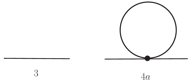
Following this strategy we now derive the two-point function for the two antiferromagnetic magnons in external fields and extract their dispersion relation. Evaluating the magnon two-point function $\tau_{\pm}(x-y)$ up to one-loop order is straightforward, because there are only two diagrams contributing, as shown in the lower panel of Fig. 1. The leading contribution (diagram 3), yields the $T$=0 propagator $\Delta_{\pm}(x-y)$ for magnon $+$ and magnon $-$,

$$\tau_{\pm}^{3}(x-y)=\Delta_{\pm}(x-y)=\int\!\!\frac{\mbox{d}^{d}\!p}{{(2\pi)}^{d}}\,\frac{e^{ip(x-y)}}{p_{4}^{2}+{\vec{p}\,}^{2}+M^{2}\pm 2iHp_{4}-H^{2}}\,,$$

(2.5)

regularized in the space-time dimension $d$. The magnon ”mass” $M$ is defined as

$$M^{2}=\frac{M_{s}H_{s}}{\rho_{s}}\,.$$

(2.6)

The only correction comes from one-loop graph 4a and reads

$$\tau_{\pm}^{4a}(x-y)=\pm\frac{2iH}{\rho_{s}}\,\Delta(0)\,\int\!\!\frac{\mbox{d}^{d}\!p}{{(2\pi)}^{d}}\,\frac{p_{4}\,e^{ip(x-y)}}{{(p_{4}^{2}+{\vec{p}\,}^{2}+M^{2}\pm 2iHp_{4}-H^{2})}^{2}}\,,$$

(2.7)

and can be embedded into the physical two-point function $\tau_{\pm}(x-y)$ via

	$\displaystyle\tau_{\pm}(x-y)$	$\displaystyle=$	$\displaystyle\int\!\!\frac{\mbox{d}^{d}\!p}{{(2\pi)}^{d}}\,\frac{e^{ip(x-y)}}{p_{4}^{2}+{\vec{p}\,}^{2}+M^{2}\pm 2iHp_{4}-H^{2}+X_{\pm}}$		(2.8)
		$\displaystyle=$	$\displaystyle\int\!\!\frac{\mbox{d}^{d}\!p}{{(2\pi)}^{d}}\,\frac{e^{ip(x-y)}}{p_{4}^{2}+{\vec{p}\,}^{2}+M^{2}\pm 2iHp_{4}-H^{2}}$
			$\displaystyle\times\Bigg\{1-\frac{X_{\pm}}{p_{4}^{2}+{\vec{p}\,}^{2}+M^{2}\pm 2iHp_{4}-H^{2}}+{\cal O}(X^{2}/{\cal D}^{2})\Bigg\}\,.$

The quantity $\Delta(0)$ in Eq. (2.7) is the dimensionally regularized zero-temperature magnon propagator at the coordinate origin $x$=0 when no magnetic field is present,

$$\Delta(0)=\int\frac{{\mbox{d}}^{d}p}{{(2\pi)}^{d}}\,\frac{1}{p^{2}+M^{2}}={\int}_{\!\!\!0}^{\infty}\mbox{d}\rho\,(4\pi\rho)^{-d/2}e^{-\rho M^{2}}\,.$$

(2.9)

While the dispersion relation

$${\cal D}=p_{4}^{2}+{\vec{p}\,}^{2}+M^{2}\pm 2iHp_{4}-H^{2}$$

(2.10)

is tied to the leading order propagator $\Delta_{\pm}(x-y)$, the correction $X_{\pm}$ takes into account the next-to-leading order contribution $\tau_{\pm}^{4a}(x-y)$.

The physical limit $d\to 3$ can be taken without problems: the quantity $\Delta(0)$ is not singular in two spatial dimensions, but remains finite when the regularization is removed,

$$\lim_{d\to 3}\Delta(0)=-\frac{M}{4\pi}=-\frac{\sqrt{M_{s}H_{s}}}{4\pi\sqrt{\rho_{s}}}\,,$$

(2.11)

such that the dispersion relations for the ”dressed” magnons take the form

$$\omega_{\pm}=\sqrt{{\vec{p}\,}^{2}+\frac{M_{s}H_{s}}{\rho_{s}}+\frac{H^{2}\sqrt{M_{s}H_{s}}}{2\pi\rho^{\frac{3}{2}}_{s}}}\pm H\pm\frac{H\sqrt{M_{s}H_{s}}}{4\pi\rho^{\frac{3}{2}}_{s}}\,.$$

(2.12)

On the basis of these relations we can now determine the portion in the free energy density that is associated with noninteracting magnons by means of

$$z^{free}=z_{0}^{free}+\frac{T}{{(2\pi)}^{2}}\,\int\!\!\mbox{d}^{2}\!p\,\ln\Big[1-e^{-\omega_{+}({\vec{p}})/T}\Big]+\frac{T}{{(2\pi)}^{2}}\,\int\!\!\mbox{d}^{2}\!p\,\ln\Big[1-e^{-\omega_{-}({\vec{p}})/T}\Big]\,,$$

(2.13)

where $z_{0}^{free}$ is the vacuum energy density of the noninteracting magnons. The corrections to the leading order dispersion law appear as

$$\omega_{\pm}({\vec{p}})=\sqrt{{\vec{p}\,}^{2}+\frac{M_{s}H_{s}}{\rho_{s}}+\epsilon^{A}_{\pm}}\pm H+\epsilon^{B}_{\pm}\,.$$

(2.14)

We thus consider the pertinent expansions

	$\displaystyle\exp\!\Big(-\frac{\omega_{\pm}}{T}\Big)$	$\displaystyle\approx$	$\displaystyle\exp\!\Big(-\frac{\omega_{0}\pm H}{T}\Big)\Bigg\{1-\frac{\epsilon^{B}_{\pm}}{T}-\frac{\epsilon^{A}_{\pm}}{2\omega_{0}T}+{\cal O}(\epsilon^{2})\Bigg\}\,,$		(2.15)
			$\displaystyle\omega_{0}=\sqrt{{\vec{p}\,}^{2}+\frac{M_{s}H_{s}}{\rho_{s}}}\,,$

and

	$\displaystyle\ln\!\Big(1-e^{-\frac{\omega_{\pm}}{T}}\Big)$	$\displaystyle\approx$	$\displaystyle\ln\!\Big(1-e^{-(\omega_{0}\pm H)/T}\Big)$		(2.16)
			$\displaystyle+\frac{1}{T}\,\Bigg\{\epsilon^{B}_{\pm}+\frac{\epsilon^{A}_{\pm}}{2\omega_{0}}\Bigg\}\,\frac{1}{e^{(\omega_{0}\pm H)/T}-1}\,,$

integrate over momentum according to Eq. (2.13), and end up with the portion in the free energy density that is due to noninteracting magnons:

$$z^{free}=-{\hat{h}}_{0}\,T^{3}-\frac{\sqrt{M_{s}H_{s}}H}{4\pi\rho_{s}^{3/2}}\,\frac{\partial{\hat{h}}_{0}}{\partial H}\,T^{3}+\frac{\sqrt{M_{s}H_{s}}H^{2}}{2\pi\rho_{s}^{3/2}}\,{\hat{h}}_{1}\,T+z^{free}_{0}\,.$$

(2.17)

The kinematical functions ${\hat{h}}_{0}$ (or equivalently: ${\hat{g}}_{0})$ and ${\hat{h}}_{1}$ (or equivalently: ${\hat{g}}_{1})$ are

	$\displaystyle{\hat{h}}_{0}$	$\displaystyle=$	$\displaystyle\frac{{\hat{g}}_{0}}{T^{3}}$		(2.18)
		$\displaystyle=$	$\displaystyle-\frac{1}{2\pi T^{2}}\int_{0}^{\infty}\!\!\mbox{d}p\,p\,\Bigg\{\ln\Big[1-e^{-(\sqrt{p^{2}+M^{2}}+H)/T}\Big]+\ln\Big[1-e^{-(\sqrt{p^{2}+M^{2}}-H)/T}\Big]\Bigg\}$
		$\displaystyle=$	$\displaystyle\frac{1}{4\pi T^{3}}\!\int_{0}^{\infty}\!\!\mbox{d}p\,p^{3}\,\frac{1}{\sqrt{p^{2}+M^{2}}}\,\Bigg\{\frac{1}{e^{(\sqrt{p^{2}+M^{2}}+H)/T}-1}+\frac{1}{e^{(\sqrt{p^{2}+M^{2}}-H)/T}-1}\Bigg\}\,,$

and

	$\displaystyle{\hat{h}_{1}}$	$\displaystyle=$	$\displaystyle\frac{{\hat{g}}_{1}}{T}$		(2.19)
		$\displaystyle=$	$\displaystyle\frac{1}{4\pi T}\!\int_{0}^{\infty}\!\!\mbox{d}p\,p\,\frac{1}{\sqrt{p^{2}+M^{2}}}\,\Bigg\{\frac{1}{e^{(\sqrt{p^{2}+M^{2}}+H)/T}-1}+\frac{1}{e^{(\sqrt{p^{2}+M^{2}}-H)/T}-1}\Bigg\}\,,$

respectively.

We are now able to extract the genuine spin-wave interaction part $z^{int}$ in the free energy density that is given by the difference between the total two-loop free energy density $z$, derived in Ref. [55],

	$\displaystyle z$	$\displaystyle=$	$\displaystyle z_{0}-{\hat{g}}_{0}+\frac{H}{\rho_{s}}\,{\hat{g}}_{1}\,\frac{\partial{\hat{g}}_{0}}{\partial H}-\frac{\sqrt{M_{s}H_{s}}H}{4\pi\rho_{s}^{3/2}}\,\frac{\partial{\hat{g}}_{0}}{\partial H}-\frac{H^{2}}{\rho_{s}}{({\hat{g}}_{1})}^{2}+\frac{\sqrt{M_{s}H_{s}}H^{2}}{2\pi\rho_{s}^{3/2}}\,{\hat{g}}_{1}\,,$		(2.20)
			$\displaystyle z_{0}=-M_{s}H_{s}-\frac{M^{3/2}_{s}H^{3/2}_{s}}{6\pi\rho_{s}^{3/2}}-(k_{2}+k_{3})\frac{M^{2}_{s}H^{2}_{s}}{\rho_{s}^{2}}-\frac{M_{s}H_{s}H^{2}}{16\pi^{2}\rho_{s}^{2}}\,,$

and the piece $z^{free}$, Eq. (2.17), as

$$z^{int}=z-z^{free}\,.$$

(2.21)

We obtain the simple result

	$\displaystyle z^{int}$	$\displaystyle=$	$\displaystyle\frac{H}{\rho_{s}}\,{\hat{h}}_{1}\,\frac{\partial{\hat{h}}_{0}}{\partial H}\,T^{4}-\frac{H^{2}}{\rho_{s}}\,{({\hat{h}}_{1})}^{2}\,T^{2}+z^{int}_{0}$		(2.22)
			$\displaystyle z^{int}_{0}=-\frac{M_{s}H_{s}H^{2}}{16\pi^{2}\rho_{s}^{2}}\,,$

and furthermore identify $z^{free}_{0}$ as

$$z^{free}_{0}=-M_{s}H_{s}-\frac{M^{3/2}_{s}H^{3/2}_{s}}{6\pi\rho_{s}^{3/2}}-(k_{2}+k_{3})\frac{M^{2}_{s}H^{2}_{s}}{\rho_{s}^{2}}\,.$$

(2.23)

The vacuum energy density involves the next-to-leading order effective constants $k_{2}$ and $k_{3}$. It should be emphasized that in two spatial dimensions these are only relevant at zero temperature.⁴⁴ 4 Besides, numerically they are small. For the spin-$\frac{1}{2}$ square-lattice antiferromagnet the value of the relevant combination $k_{2}+k_{3}$ is known from Monte Carlo simulations [61]: $(k_{2}+k_{3})/v^{2}=-0.0018\,\rho_{s}^{-1}=-0.0102\,J^{-1}$. The finite-temperature physics of the system, up to two-loop order, is fully described in terms of the leading order effective constants $\rho_{s}$ and $M_{s}$. The only difference between, e.g., square and honeycomb lattice antiferromagnets consists in the concrete values of $\rho_{s}$ and $M_{s}$. For the spin-$\frac{1}{2}$ square-lattice antiferromagnet they are (see, e.g., Ref. [61])

$$\rho_{s}=0.1808(4)J\,,\quad M_{s}=0.30743(1)/a^{2}\,,\quad v=1.6585(10)Ja\,,$$

(2.24)

for the spin-$\frac{1}{2}$ honeycomb-lattice antiferromagnet, according to Ref. [62], we have

$$\rho_{s}=0.102(2)J\,,\quad{\tilde{M}_{s}}=0.2688(3)\,,\quad v=1.297(16)Ja\,,$$

(2.25)

where

$${\tilde{M}_{s}}=\frac{3\sqrt{3}}{4}\,M_{s}\,a^{2}\,.$$

(2.26)

Note that we also quote the respective values for the spin-wave velocity $v$.

In three spatial dimensions, each additional magnon loop corresponds to a suppression of two powers of temperature. The diagrams for the free energy density we need to evaluate up to two-loop order, are depicted in the upper panel of Fig. 2. Comparing with the relevant diagrams for two-dimensional antiferromagnets, we note that here two additional diagrams emerge: the one-loop graph $6B$ and the tree graph $6C$. The leading finite-temperature contribution (order $T^{4}$) stems from the one-loop graph $4A$. At next-to-leading order we have two finite-temperature contributions (order $T^{6}$) coming from the two-loop graph 6A and the one-loop graph 6B.⁵⁵ 5 Details on the effective loop evaluation can be found in Ref. [57].

To isolate the genuine magnon-magnon interaction portion in the free energy density, we follow the same strategy as before: we represent the free energy density in terms of the dressed quasiparticles by evaluating the two-point function and the dispersion relation for both antiferromagnetic magnons. The relevant diagrams for the two-point function $\tau_{\pm}(x-y)$ are shown in the lower panel of Fig. 2.

The leading contribution (diagram 4) corresponds to the zero-temperature propagator $\Delta_{\pm}(x-y)$ for magnon $+$ and magnon $-$,

$$\tau_{\pm}^{4}(x-y)=\Delta_{\pm}(x-y)=\int\!\!\frac{\mbox{d}^{d}\!p}{{(2\pi)}^{d}}\,\frac{e^{ip(x-y)}}{p_{4}^{2}+{\vec{p}\,}^{2}+M^{2}\pm 2iHp_{4}-H^{2}}\,.$$

(2.27)

The correction from the one-loop graph 6A is the same as for the quantities $\tau_{\pm}^{4a}(x-y)$, Eq. (2.7),

$$\tau_{\pm}^{6A}(x-y)=\pm\frac{2iH}{\rho_{s}}\,\Delta(0)\,\int\!\!\frac{\mbox{d}^{d}\!p}{{(2\pi)}^{d}}\,\frac{p_{4}\,e^{ip(x-y)}}{{(p_{4}^{2}+{\vec{p}\,}^{2}+M^{2}\pm 2iHp_{4}-H^{2})}^{2}}\,,$$

(2.28)

with the exception that the dimensionally regularized expression $\Delta(0)$ diverges when the physical limit $d\to 4$ is taken. This apparent dilemma is solved by the observation that the additional contribution from the tree graph $6B$,

	$\displaystyle\tau_{\pm}^{6B}(x-y)$	$\displaystyle=$	$\displaystyle-\frac{2(k_{2}-k_{1})M^{4}}{\rho_{s}}\,\int\!\!\frac{\mbox{d}^{d}\!p}{{(2\pi)}^{d}}\,\frac{e^{ip(x-y)}}{{(p_{4}^{2}+{\vec{p}\,}^{2}+M^{2}\pm 2iHp_{4}-H^{2})}^{2}}$		(2.29)
			$\displaystyle\pm\frac{4ik_{1}M^{2}H}{\rho_{s}}\,\int\!\!\frac{\mbox{d}^{d}\!p}{{(2\pi)}^{d}}\,\frac{p_{4}\,e^{ip(x-y)}}{{(p_{4}^{2}+{\vec{p}\,}^{2}+M^{2}\pm 2iHp_{4}-H^{2})}^{2}}\,,$

also becomes singular in the limit $d\to 4$ and that the divergences mutually cancel as we now show.

The divergence in the zero-temperature propagator at the coordinate origin, $\Delta(0)$,

$$\Delta(0)=\int\frac{{\mbox{d}}^{d}p}{{(2\pi)}^{d}}\,\frac{1}{p^{2}+M^{2}}={\int}_{\!\!\!0}^{\infty}\mbox{d}\rho\,(4\pi\rho)^{-d/2}e^{-\rho M^{2}}=2M^{2}\lambda\,,$$

(2.30)

is contained in the parameter $\lambda$,

	$\displaystyle\lambda$	$\displaystyle=$	$\displaystyle\mbox{$\frac{1}{2}$}\,(4\pi)^{-d/2}\,\Gamma(1-{\mbox{$\frac{1}{2}$}}d)M^{d-4}$		(2.31)
		$\displaystyle=$	$\displaystyle\frac{M^{d-4}}{16{\pi}^{2}}\,\Bigg[\frac{1}{d-4}-\mbox{$\frac{1}{2}$}\{\ln{4{\pi}}+{\Gamma}^{\prime}(1)+1\}+{\cal O}(d-4)\Bigg]\,.$

On the other hand, the singularity in diagram $6B$ is due to the presence of NLO effective constants. Following Ref. [52, 57], these can be written as

$$k_{1}={\tilde{\gamma}}_{3}\Big(\lambda+\frac{{\overline{k}}_{1}}{32\pi^{2}}\Big)\,,\quad k_{2}={\tilde{\gamma}}_{4}\Big(\lambda+\frac{{\overline{k}}_{2}}{32\pi^{2}}\Big)\,,$$

(2.32)

with coefficients

$${\tilde{\gamma}}_{3}=-1\,,\quad{\tilde{\gamma}}_{4}=-1\,.$$

(2.33)

The $\lambda$-divergences in the sum of diagrams $6A$ and $6B$ hence cancel. The renormalized NLO effective constants ${\overline{k}}_{1}$ and ${\overline{k}}_{2}$ are finite in $d=4$ and of unit order,

$${\overline{k}}_{1},{\overline{k}}_{2}\approx 1\,.$$

(2.34)

Adhering to the same steps as in the previous subsection, the magnon dispersion relations take the form

	$\displaystyle\omega_{\pm}$	$\displaystyle=$	$\displaystyle\sqrt{{\vec{p}\,}^{2}+\frac{M_{s}H_{s}}{\rho_{s}}-\frac{{\overline{k}}_{2}-{\overline{k}}_{1}}{16\pi^{2}\rho_{s}}\,{\Bigg(\frac{M_{s}H_{s}}{\rho_{s}}\Bigg)}^{2}+\frac{{\overline{k}}_{1}}{8\pi^{2}\rho_{s}}\,\frac{M_{s}H_{s}H^{2}}{\rho_{s}}}$		(2.35)
			$\displaystyle\pm H\pm\frac{{\overline{k}}_{1}}{16\pi^{2}\rho_{s}}\,\frac{M_{s}H_{s}H}{\rho_{s}}\,,$

and the piece in the free energy density that is due to noninteracting magnons amounts to

	$\displaystyle z^{free}$	$\displaystyle=$	$\displaystyle-{\hat{h}}_{0}\,T^{4}-\frac{{\overline{k}}_{2}-{\overline{k}}_{1}}{16\pi^{2}}\frac{M^{2}_{s}H^{2}_{s}}{\rho^{3}_{s}}\,{\hat{h}}_{1}T^{2}-\frac{{\overline{k}}_{1}}{16\pi^{2}}\,\frac{HM_{s}H_{s}}{\rho^{2}_{s}}\frac{\partial{\hat{h}}_{0}}{\partial H}\,T^{4}$		(2.36)
			$\displaystyle+\frac{{\overline{k}}_{1}}{8\pi^{2}}\,\frac{H^{2}M_{s}H_{s}}{\rho^{2}_{s}}\,{\hat{h}}_{1}T^{2}+z^{free}_{0}\,.$

The kinematical functions in three spatial dimensions, ${\hat{h}}_{0}$ (or equivalently: ${\hat{g}}_{0})$ and ${\hat{h}}_{1}$ (or equivalently: ${\hat{g}}_{1})$, are

	$\displaystyle{\hat{h}}_{0}$	$\displaystyle=$	$\displaystyle\frac{{\hat{g}}_{0}}{T^{4}}$		(2.37)
		$\displaystyle=$	$\displaystyle-\frac{1}{2\pi^{2}T^{3}}\int_{0}^{\infty}\!\!\mbox{d}p\,p^{2}\,\Bigg\{\ln\Big[1-e^{-(\sqrt{p^{2}+M^{2}}+H)/T}\Big]+\ln\Big[1-e^{-(\sqrt{p^{2}+M^{2}}-H)/T}\Big]\Bigg\}$
		$\displaystyle=$	$\displaystyle\frac{1}{6\pi^{2}T^{4}}\!\int_{0}^{\infty}\!\!\mbox{d}p\,p^{4}\,\frac{1}{\sqrt{p^{2}+M^{2}}}\,\Bigg\{\frac{1}{e^{(\sqrt{p^{2}+M^{2}}+H)/T}-1}+\frac{1}{e^{(\sqrt{p^{2}+M^{2}}-H)/T}-1}\Bigg\}\,,$

and

	$\displaystyle{\hat{h}_{1}}$	$\displaystyle=$	$\displaystyle\frac{{\hat{g}}_{1}}{T^{2}}$		(2.38)
		$\displaystyle=$	$\displaystyle\frac{1}{4\pi^{2}T^{2}}\!\int_{0}^{\infty}\!\!\mbox{d}p\,p^{2}\,\frac{1}{\sqrt{p^{2}+M^{2}}}\,\Bigg\{\frac{1}{e^{(\sqrt{p^{2}+M^{2}}+H)/T}-1}+\frac{1}{e^{(\sqrt{p^{2}+M^{2}}-H)/T}-1}\Bigg\}\,,$

respectively.

Resorting to the renormalized representation for the total two-loop free energy density, derived in Ref. [57],

	$\displaystyle z$	$\displaystyle=$	$\displaystyle z_{0}-{\hat{g}}_{0}+\frac{H}{\rho_{s}}\,{\hat{g}}_{1}\,\frac{\partial{\hat{g}}_{0}}{\partial H}-\frac{H^{2}}{\rho_{s}}{({\hat{g}}_{1})}^{2}-\frac{{\overline{k}}_{2}-{\overline{k}}_{1}}{16\pi^{2}}\frac{M^{2}_{s}H^{2}_{s}}{\rho^{3}_{s}}\,{\hat{g}}_{1}-\frac{{\overline{k}}_{1}}{16\pi^{2}}\,\frac{HM_{s}H_{s}}{\rho^{2}_{s}}\frac{\partial{\hat{g}}_{0}}{\partial H}$		(2.39)
			$\displaystyle+\frac{{\overline{k}}_{1}}{8\pi^{2}}\,\frac{H^{2}M_{s}H_{s}}{\rho^{2}_{s}}\,{\hat{g}}_{1}\,,$
			$\displaystyle z_{0}=-M_{s}H_{s}+\frac{{\overline{k}}_{2}-2{\overline{k}}_{3}}{32\pi^{2}}\,\frac{M^{2}_{s}H^{2}_{s}}{\rho^{2}_{s}}-\frac{M^{2}_{s}H^{2}_{s}}{64\pi^{2}\rho^{2}_{s}}+{\cal O}(p^{6})\,,$

we extract the genuine spin-wave interaction part $z^{int}$ as

	$\displaystyle z^{int}$	$\displaystyle=$	$\displaystyle\frac{H}{\rho_{s}}\,{\hat{h}}_{1}\,\frac{\partial{\hat{h}}_{0}}{\partial H}\,T^{6}-\frac{H^{2}}{\rho_{s}}\,{({\hat{h}}_{1})}^{2}\,T^{4}+z^{int}_{0}$		(2.40)
			$\displaystyle z^{int}_{0}={\cal O}(p^{6})\,.$

The renormalized NLO effective constant ${\overline{k}}_{3}$, much like ${\overline{k}}_{1}$ and ${\overline{k}}_{2}$, is of natural order, i.e., ${\overline{k}}_{3}\approx 1$.

Finally, we identify the vacuum energy density associated with noninteracting magnons as

$$z^{free}_{0}=-M_{s}H_{s}+\frac{{\overline{k}}_{2}-2{\overline{k}}_{3}}{32\pi^{2}}\,\frac{M^{2}_{s}H^{2}_{s}}{\rho^{2}_{s}}-\frac{M^{2}_{s}H^{2}_{s}}{64\pi^{2}\rho^{2}_{s}}\,.$$

(2.41)

Unlike for antiferromagnetic films, in three spatial dimensions, NLO effective constants also show up in the finite-temperature piece $z-z_{0}$ according to Eq. (2.39). The remainder ${\cal O}(p^{6})$ of the zero-temperature contribution $z_{0}$ even contains NNLO effective constants that originate from the tree graph $6C$ of Fig. 2. The corresponding terms in the vacuum energy density are of the form $\propto H_{s}^{3},\propto H_{s}^{2}H^{2},\propto H_{s}H^{4}$ and $\propto H^{6}$, where each such term contains a linear combination of NNLO effective constants, much like the second term in Eq. (2.41) involves the combination ${\overline{k}}_{2}-2{\overline{k}}_{3}$ of NLO effective constants. But because the numerical values of NNLO effective constants are very small – and their sign a priori unknown – we refrain from providing a lenghty explicit expression for all these higher-order contributions that only matter at zero temperature.

It should be stressed that the finite-temperature interaction contribution $z^{int}-z^{int}_{0}$ is free of such NLO (or NNLO) quantities. As in the case of antiferromagnetic films, it only depends on the spin stiffness $\rho_{s}$ and the order parameter $M_{s}$. This implies that the question of whether the magnon-magnon interaction in the pressure leads to attraction or repulsion, can be answered in a model-independent – and thus universal – way also in three spatial dimensions.

The thermodynamic quantities depend on three parameters: $T,H_{s},H$. Magnon effective field theory is valid in the sector where these quantities are small, i.e., small with respect to the exchange integral $J$ that defines the non-thermal microscopic scale in the underlying Hamiltonian.

Rather than operating with the dimensionful quantities $T,H_{s},H$, we define three dimensionless parameters as

$$t\equiv\frac{T}{2\pi\rho_{s}}\,,\qquad m\equiv\frac{\sqrt{M_{s}H_{s}}}{2\pi\rho_{s}^{3/2}}\,,\qquad m_{H}\equiv\frac{H}{2\pi\rho_{s}}\,.$$

(3.1)

Note that the common denominator,

$$2\pi\rho_{s}\approx J\,,$$

(3.2)

approximately concurs with the exchange coupling $J$, such that $t,m,m_{H}$ must be small. In concrete plots we choose the parameter region as

$$t,m,m_{H}\ \lesssim 0.4\,.$$

(3.3)

In addition, we implement the stability criterion, Eq. (2.4), by

$$m>m_{H}+\delta\,,\qquad\delta=0.1\,.$$

(3.4)

The low-temperature series for the pressure, i.e., the negative of the temperature-dependent part of the free energy density,

$$P=z_{0}-z\,,$$

(3.5)

takes the form

$$P(t,m,m_{H})=p_{1}T^{3}+p_{2}T^{4}+{\cal O}(T^{5})\,.$$

(3.6)

The coefficient $p_{1}$ of the dominant piece ($\propto T^{3}$) stems from noninteracting dressed magnons and reads

$$p_{1}={\hat{h}}_{0}+\frac{mm_{H}}{2}\,\frac{\partial{\hat{h}}_{0}}{\partial m_{H}}-\frac{mm_{H}^{2}}{t^{2}}\,{\hat{h}}_{1}\,,$$

(3.7)

while interaction effects are contained in the order-$T^{4}$ contribution with coefficient

$$p_{2}=\Bigg\{-2\pi m_{H}t\,{\hat{h}}_{1}\frac{\partial{\hat{h}}_{0}}{\partial m_{H}}+\frac{2\pi m_{H}^{2}}{t}\,{({\hat{h}}_{1})}^{2}\Bigg\}\,\frac{1}{2\pi\rho_{s}t}\,.$$

(3.8)

To explore the effect of the magnon-magnon interaction in the pressure, we define the dimensionless ratio between interaction piece and free dressed magnon gas as

$$P_{int}=\frac{p_{2}T^{4}}{p_{1}T^{3}}=2\pi\rho_{s}t\,\frac{p_{2}}{p_{1}}\,.$$

(3.9)

In Fig. 3, for a bipartite two-dimensional antiferromagnet at the temperatures $t=0.2$ and $t=0.4$, the ratio $P_{int}$ is plotted as a function of magnetic ($m_{H}$) and staggered ($m$) field strength.⁶⁶ 6 Note that the spin stiffness $\rho_{s}$ drops out in the ratio $P_{int}$: we are hence dealing with a universal parametrization valid for a generic two-dimensional bipartite antiferromagnet. One observes that the interaction in stronger fields is quite large, amounting up to about fifteen percent compared to the noninteracting magnon gas contribution. In the entire parameter space we consider, the genuine spin-wave interaction in the pressure is attractive and tends to zero when the magnetic field is turned off.

In Fig. 4, for the same temperatures $t=0.2$ and $t=0.4$, we show the full two-loop representation for the pressure, i.e., the quantity

$$p_{1}T^{3}+p_{2}T^{4}\,,$$

(3.10)

specifically for the spin-$\frac{1}{2}$ square-lattice antiferromagnet. One identifies two opposite tendencies: the pressure grows as the magnetic field gets stronger, but the pressure drops when the staggered field increases. It should be noted that the pressure – up to two-loop order – does not involve any microscopic quantities other than $\rho_{s}$ and $M_{s}$.⁷⁷ 7 $M_{s}$ is hidden in the low-energy parameter $m$.

To define analogous low-energy parameters $t,m,m_{H}$ for antiferromagnets in three spatial dimensions, we consider the simple cubic spin-$\frac{1}{2}$ antiferromagnet, where spin stiffness and exchange integral are connected by (see Ref. [46])

$$\sqrt{\rho_{s}}\approx 0.61|J|\,.$$

(3.11)

Accordingly, the three dimensionless parameters we define as

$$t\equiv\frac{T}{\sqrt{\rho_{s}}}\,,\qquad m\equiv\frac{\sqrt{M_{s}H_{s}}}{\rho_{s}}\,,\qquad m_{H}\equiv\frac{H}{\sqrt{\rho_{s}}}\,.$$

(3.12)

Here we choose the parameter range as

$$t,\,m,\,m_{H}\ \lesssim 0.6\,,$$

(3.13)

and implement the stability criterion, Eq. (2.4), again by

$$m>m_{H}+\delta\,,\qquad\delta=0.1\,.$$

(3.14)

The low-temperature expansion of the pressure for three-dimensional antiferromagnets takes the structure

$$P(t,m,m_{H})=p_{1}T^{4}+p_{2}T^{6}+{\cal O}(T^{8})\,.$$

(3.15)

The coefficient $p_{1}$ of the dominant piece refers to noninteracting dressed magnons,

$$p_{1}={\hat{h}}_{0}+\frac{{\overline{k}}_{2}-{\overline{k}}_{1}}{16\pi^{2}}\,\frac{m^{4}}{t^{2}}\,{\hat{h}}_{1}+\frac{{\overline{k}}_{1}}{16\pi^{2}}\,m^{2}m_{H}\frac{\partial{\hat{h}}_{0}}{\partial m_{H}}-\frac{{\overline{k}}_{1}}{8\pi^{2}}\,\frac{m^{2}m^{2}_{H}}{t^{2}}\,{\hat{h}}_{1}\,,$$

(3.16)

while the subsequent contribution of order $T^{6}$,

$$p_{2}=\frac{1}{\rho_{s}t^{2}}\,\Bigg\{-m_{H}t^{2}\,{\hat{h}}_{1}\,\frac{\partial{\hat{h}}_{0}}{\partial m_{H}}+m^{2}_{H}\,{({\hat{h}}_{1})}^{2}\Bigg\}\,,$$

(3.17)

corresponds to the magnon-magnon interaction.

The leading coefficient $p_{1}$ is dominated by the kinematical function ${\hat{h}}_{0}$: the remaining terms that contain the NLO effective constants ${\overline{k}}_{1}$ and ${\overline{k}}_{2}$ are small. Since only order of magnitude of ${\overline{k}}_{1}$ and ${\overline{k}}_{2}$ is known – but not their exact numerical values for concrete physical samples – in our assessment of the magnon-magnon interaction we consider the dimensionless ratio

$$P_{int}=\frac{p_{2}T^{6}}{{\hat{h}}_{0}T^{4}}=\rho_{s}t^{2}\,\frac{p_{2}}{{\hat{h}}_{0}}\,.$$

(3.18)

In Fig. 5, for a generic bipartite three-dimensional antiferromagnet at the temperatures $t=0.2$ and $t=0.4$, the ratio $P_{int}$ is plotted as a function of magnetic ($m_{H}$) and staggered ($m$) field strength. In contrast to the two-dimensional case, here the interaction is rather weak: even in stronger fields it only amounts up to about one percent compared to the noninteracting magnon gas. But we find that the genuine spin-wave interaction in the pressure is attractive also in the case of three-dimensional antiferromagnets and that it tends to zero when the magnetic field is turned off.

For the same temperatures $t=0.2$ and $t=0.4$, in Fig. 6, we show the full two-loop representation for the pressure, i.e., the quantity

$$p_{1}T^{4}+p_{2}T^{6}$$

(3.19)

for the simple cubic spin-$\frac{1}{2}$ antiferromagnet. As before we identify two opposite tendencies: the pressure grows when the magnetic field gets stronger, but the pressure drops as the staggered field increases.

One final comment is in order here. Fig. 6 refers to the simple cubic spin-$\frac{1}{2}$ antiferromagnet where the numerical value of the spin stiffness, Eq. (3.11), is known. However, we are unaware of the precise values of the NLO effective constants ${\overline{k}}_{1}$ and ${\overline{k}}_{2}$. But since we know that their magnitude is of order one, we can perform a scan of these quantities in the interval

$$\{{\overline{k}}_{1},{\overline{k}}_{2}\}\ \subset\ [-5,5]\,,$$

(3.20)

which gives us a set of surfaces for the pressure $P(t,m,m_{H})$. From these scans we then select the respective two extreme situations: maximal and minimal corrections for each point in parameter space $(t,m,m_{H})$. These two surfaces represent estimates of upper and lower bounds for the corrections that are due to ${\overline{k}}_{1}$ and ${\overline{k}}_{2}$. As witnessed by Fig. 6, these two extreme hypersurfaces can barely be distinguished even in stronger fields, i.e., the corrections involving NLO effective constants are indeed very small.

References

- Kubo [1952] R. Kubo, Phys. Rev. 87, 568 (1952).
- Oguchi [1960] T. Oguchi, Phys. Rev. 117, 117 (1960).
- Joenk [1962] R. J. Joenk, Phys. Rev. 128, 1634 (1962).
- Takahashi [1989] M. Takahashi, Phys. Rev. B 40, 2494 (1989).
- Hamer et al. [1992] C. J. Hamer, Z. Weihong, and P. Arndt, Phys. Rev. B 46, 6276 (1992).
- Antsygina and Slyusarev [1993] T. N. Antsygina and V. A. Slyusarev, Theor. Math. Phys. 95, 424 (1993).
- Zhitomirsky and Nikuni [1998a] M. E. Zhitomirsky and T. Nikuni, Phys. Rev. B 57, 5013 (1998).
- Zhitomirsky and Nikuni [1998b] M. E. Zhitomirsky and T. Nikuni, Physica B 241-243, 573 (1998).
- Spremo et al. [2005] I. Spremo, F. Schütz, P. Kopietz, V. Pashchenko, B. Wolf, M. Lang, J. W. Bats, C. Hu, and M. U. Schmidt, Phys. Rev. B 72, 174429 (2005).
- Hasselmann et al. [2007] N. Hasselmann, F. Schütz, I. Spremo, and P. Kopietz, C. R. Chimie 10, 60 (2007).
- Kreisel et al. [2008] A. Kreisel, F. Sauli, N. Hasselmann, and P. Kopietz, Phys. Rev. B 78, 035127 (2008).
- Morozov [1972] V. G. Morozov, Phys. Stat. Sol. (b) 50, 479 (1972).
- Ghosh [1973] D. K. Ghosh, Phys. Rev. B 8, 392 (1973).
- Lymar and Rudoi [1974] V. I. Lymar and Y. G. Rudoi, Theor. Math. Phys. 21, 990 (1974).
- Lymar and Rudoi [1975] V. I. Lymar and Y. G. Rudoi, Theor. Math. Phys. 24, 912 (1975).
- Wei et al. [2014] W. Qin, H.-Y. Wang, and G.-L. Long, Chin. Phys. B 23, 037502 (2014).
- Hamer et al. [1991] Z. Weihong, J. Oitmaa, and C. J. Hamer, Phys. Rev. B 43, 8321 (1991).
- Pan [1998] K.-K. Pan, Phys. Lett. A 244, 169 (1998).
- Pan [1999] K.-K. Pan, Phys. Rev. B 59, 1168 (1999).
- Pan [2000] K.-K. Pan, Phys. Lett. A 271, 291 (2000).
- Sandvik [1999] A. W. Sandvik, Phys. Rev. B 59, R14157 (1999).
- Syljuasen and Sandvik [2002] O. F. Syljuasen and A. W. Sandvik, Phys. Rev. E 66, 046701 (2002).
- Palma and Riveros [2015] G. Palma and A. Riveros, Condens. Matter Phys. 18, 23002 (2015).
- Fabricius et al. [1992] K. Fabricius, M. Karbach, U. Löw, and K.-H. Mütter, Phys. Rev. B 45, 5315 (1992).
- Luescher and Laeuchli [2009] A. Lüscher and A. M. Läuchli, Phys. Rev. B 79, 195102 (2009).
- Falk [1964] H. Falk, Phys. Rev. 133, A1382 (1964).
- Pikalev et al. [1969] E. M. Pikalev, M. A. Savchenko, and J. Solyom, Sov. Phys. JETP 28, 734 (1969).
- Cottam and Stinchcombe [1970] M. G. Cottam and R. B. Stinchcombe, J. Phys. C: Solid St. Phys. 3, 2283 (1970).
- Morozov and Mukhai [1979] V. G. Morozov and A. N. Mukhai, Theor. Math. Phys. 36, 624 (1978).
- Brajczewska et al. [1990] M. Brajczewska, C. Fiolhais, and J. da Providencia, Physica B 160, 357 (1990).
- Gluzman [1993] S. Gluzman, Z. Phys. B 90, 313 (1993).
- Sachdev et al. [1994] S. Sachdev, T. Senthil, and R. Shankar, Phys. Rev. B 50, 258 (1994).
- Bublitz and de Sousa [2004] E. Bublitz and J. R. de Sousa, J. Magn. Mag. Mat. 269, 266 (2004).
- Filho and de Sousa [2004] E. B. Filho and J. R. de Sousa, Phys. Lett. A 323, 9 (2004).
- Neto and de Sousa [2007] J. C. Neto and J. R. de Sousa, Solid State Comm. 144, 470 (2007).
- Vogt and Kettemann [2009] B. Vogt and S. Kettemann, Ann. Phys. (Berlin) 18, 759 (2009).
- Neto et al. [2018] M. A. Neto, J. R. Viana, O. D. R. Salmon, E. B. Filho, and J. R. de Sousa, Mod. Phys. Lett. B 32, 1850390 (2018).
- Halperin and Hohenberg [1969] B. I. Halperin and P. C. Hohenberg, Phys. Rev. 188, 898 (1969).
- Chakravarty et al. [1989] S. Chakravarty, B. I. Halperin, and D. R. Nelson, Phys. Rev. B 39, 2344 (1989).
- Neuberger and Ziman [1989] H. Neuberger and T. Ziman, Phys. Rev. B 39, 2608 (1989).
- Fisher [1989] D. S. Fisher, Phys. Rev. B 39, 11783 (1989).
- Hasenfratz and Leutwyler [1990] P. Hasenfratz and H. Leutwyler, Nucl. Phys. B 343, 241 (1990).
- Hasenfratz and Niedermayer [1993] P. Hasenfratz and F. Niedermayer, Z. Phys. B 92, 91 (1993).
- Leutwyler [1994a] H. Leutwyler, Phys. Rev. D 49, 3033 (1994).
- Hofmann [1999] C. P. Hofmann, Phys. Rev. B 60, 388 (1999).
- Hofmann [1999] C. P. Hofmann, Phys. Rev. B 60, 406 (1999).
- Roman and Soto [1999a] J. M. Román and J. Soto, Int. J. Mod. Phys. B 13, 755 (1999).
- Roman and Soto [1999b] J. M. Román and J. Soto, Ann. Phys. 273, 37 (1999).
- Roman and Soto [2000] J. M. Román and J. Soto, Phys. Rev. B 62, 3300 (2000).
- Hofmann [2010] C. P. Hofmann, Phys. Rev. B 81, 014416 (2010).
- Hofmann [2017] C. P. Hofmann, Phys. Rev. B 95, 134402 (2017).
- Hofmann [2017b] C. P. Hofmann, Nucl. Phys. B 916, 254 (2017).
- Brauner and Hofmann [2017] T. Brauner and C. P. Hofmann, Ann. Phys. 386, 178 (2017).
- Brauner and Hofmann [2020] T. Brauner and C. P. Hofmann, Ann. Phys. 418, 168168 (2020).
- Hofmann [2020a] C. P. Hofmann, J. Stat. Mech. (2020) 033103.
- Hofmann [2020b] C. P. Hofmann, Physica B 595, 412374 (2020).
- Hofmann [2020c] C. P. Hofmann, arXiv:2002.02958.
- Hofmann [2020d] C. P. Hofmann, arXiv:2008.12423.
- Akhiezer et al. [1961] A. I. Akhiezer, V. G. Baryakhtar, and M. I. Kaganov, Sov. Phys. Usp. 3, 567 (1961).
- Nolting [1986] W. Nolting, Quantentheorie des Magnetismus (Teubner, Stuttgart, 1986), Band 2.
- Gerber et al. [2009] U. Gerber, C. P. Hofmann, F.-J. Jiang, M. Nyfeler, and U.-J. Wiese, J. Stat. Mech. (2009) P03021.
- Gerber et al. [2009] F.-J. Jiang, F. Kämpfer, M. Nyfeler, and U.-J. Wiese, Phys. Rev. B 78, 214406 (2008).