Calculation of permanent magnet arrangements for stellarators: A linear least-squares method
Abstract
A problem arising in several engineering areas is to design magnets outside a volume that produce a desired magnetic field inside it. One instance of this problem is stellarator design, where it has recently been shown that permanent magnets can provide the required shaping of the magnetic field. Here we demonstrate a robust and efficient algorithm REGCOIL_PM to calculate the spatial distribution of these permanent magnets. The procedure involves a small number of fixed-point iterations, with a linear least-squares problem solved at each step. The method exploits the Biot-Savart Law’s exact linearity in magnetization density and approximate linearity in magnet size, for magnets far from the target region. No constraint is placed on the direction of magnetization, so Halbach solutions are found naturally, and the magnitude of the magnetization can be made uniformly equal to a target value.
1 Introduction
Given a desired magnetic field in some region, what arrangement of magnets outside the region can produce this field? This problem has many applications, including magnetic resonance imaging [1, 2, 3], particle accelerators [4, 5], and stellarators for magnetic confinement of plasma [6, 7, 8, 9, 10]. In stellarators, a three-dimensional magnetic field must be carefully shaped in order to provide good confinement of charged particle trajectories and meet other physics objectives. For all these applications, to design magnets one essentially needs to invert the Biot-Savart law. The Biot-Savart law provides a straightforward way to compute the magnetic field from known currents. However the inverse problem (given , determine currents) is ill-posed [9] in the sense that very different currents can give nearly the same . Therefore there is room for creativity and innovation in formulating algorithms for these inverse problems such that the magnet designs obtained are practical, and the computational cost is low.
While a variety of algorithms have been devised to compute the shapes of electromagnetic coils [6, 7, 8, 9, 10], in the area of stellarators there is much less experience with algorithms for designing permanent magnets. It has recently been demonstrated that stellarator fields can be generated at least in part by permanent magnets [11, 12, 13, 14]. Electromagnetic coils are still needed to produce a net toroidal field [11], but permanent magnets can provide the remaining field. Unlike electromagnets, permanent magnets would not require power supplies and would have greatly reduced need for cooling. Other advantages of permanent magnets for stellarators include the elimination of ripple due to discrete coils, and improved access to the plasma chamber for maintenance. Disadvantages include the inability to turn off the field, the possibility of demagnetization, and an upper limit on the achievable field strength.
In this paper we describe a new algorithm for the design of permanent magnets. We call this method REGCOIL_PM to highlight its similarity to the REGCOIL method of electromagnetic coil design [9]. REGCOIL_PM differs from some previously proposed approaches for permanent magnet design [11, 12] in that no constraint is imposed on the direction of the magnetization . Allowing the direction of to be arbitrary is expected to reduce the necessary volume of permanent magnets by approximately a factor of 2 [11]. We do however aim to constraint the magnitude , making it everywhere uniform in the magnet region, since a technical upper limit exists, roughly T for present materials.
The REGCOIL_PM algorithm is also formulated so as to be robust and fast. These features are achieved by not formulating the task as a nonlinear optimization problem. Numerical solution of nonlinear optimization problems can be fragile due to the existence of multiple local minima, with the possibility of the solver stopping in a local minimum that is not the global optimum, resulting in sensitivity to the initial condition. Indeed, dependence of the solution on the initial guess was noted in [14, 13]. Here instead we do not formulate the design problem as a nonlinear optimization problem.
The alternative approach here is motivated by the following expression for the magnetic field produced by a region of magnetization:
| (1) |
Here, the integral is performed over a region containing the permanent magnets, and is the field at position due to a magnetization (dipole moment density) at position . Then if the magnet region is considered fixed, (1) indicates that is a linear function of . Regularization is required to make the problem well-posed, but Tikhonov-like regularization can be introduced that preserves the linearity. Solving this linear problem for is naturally faster and more robust than solving a nonlinear problem, and it naturally allows the direction of to be arbitrary. (While differs slightly from the zero-field magnetization , the difference is very small for rare-Earth magnets and so will be neglected here. If desired, the material’s relationship could be inverted at each point to obtain .)
However the solution of the linear problem at fixed will have nonuniform , whereas it is preferable to have a solution with uniformly equal to the limit of the magnet material. Uniformity can be achieved by noting that the volume integral in (1) makes approximately linear in the magnet thickness. The complicated dependence on in (1) spoils this linearity, but if the magnets are not extremely close to the evaluation region, the nonlinearity will be weak. Thus, we can approximately correct the nonuniformity in by adjusting the magnet thickness. If is too large by a factor of two in a given region of , doubling the thickness of in this region (at fixed ) will result in a lowering of by approximately the same factor of two. This relationship is illustrated in figure 1. While will not be exactly uniform after this change to the shape of , the procedure can be iterated to improve the uniformity. As we will demonstrate, the number of iterations required can be quite small. While a Newton-type iteration could also be used to account for the nonlinearity, such a method would require either analytic derivatives or finite-difference derivatives, increasing the computational cost. We will show that the simpler Picard fixed-point iteration is stable and sufficient in practice.
A serious experimental design for a permanent magnet stellarator requires a detailed geometry model with many individual magnet pieces, as in [13]. Here instead we will make a crude approximation that the magnetization fills a single region with smooth curved boundaries. This smooth model roughly approximates a large number of individual magnets, but we acknowledge this approximation is likely insufficient for a serious experimental design. We make this smooth approximation here for several reasons. The primary reason is that it allows reuse of a significant amount of the REGCOIL code [9]. This made it possible to try out the idea rapidly. Second, the smooth model is numerically convenient, since it allows us to evaluate integrals with spectral accuracy using uniform grids in periodic coordinates. Having demonstrated the REGCOIL_PM algorithm in this paper, it should be straightforward to apply it in the future to more realistic geometry models with discrete magnets.
In the remainder of this paper, this REGCOIL_PM algorithm is defined in greater detail and demonstrated for several problems. Section 2 gives further detail about the mathematical formulation. Aspects of the discretization and numerical solution are discussed in section 3, using the NCSX stellarator as an example. In section 4 it is shown that our implementation reproduces the analytic solution for a Halbach cylinder. The NCSX example is developed and analyzed further in section 5, and we conclude in section 6.
2 Mathematical formulation
We consider the common 2-stage approach to stellarator design. In the first stage, the parameter space for optimization is the space of toroidal plasma boundary shapes, and the objective function is a combination of physics figures of merit for the plasma inside this boundary. In the second stage, the shapes of magnets are optimized to produce the plasma boundary shape resulting from the first stage. Our goal in this paper is to solve the stage-2 problem. If the stage-2 problem can be approximately solved quickly, the solution can be incorporated into the stage-1 objective function to penalize magnet complexity [15]. In this way, the stage-1 optimization can be made to find plasma configurations that can be supported by magnets of low complexity, and a more detailed and computationally demanding stage-2 calculation can be done for the final magnet design.
We thus focus on the problem of finding a permanent magnet arrangement to produce a desired plasma boundary surface . To state this problem precisely, first consider that must be a magnetic surface, so we wish to make everywhere on . (Matching the normal component is sufficient to ensure that the full vector coincides with the target field everywhere inside .) We then use the linearity of magnetostatics to write where is the magnetic field (1) produced by the permanent magnets and is the field produced by currents that are “fixed” during the permanent magnet design. The quantity represents contributions from the electromagnets and from current in the plasma, if there is any. Our goal can then be stated as achieving where
| (2) |
an integral over the surface of the squared normal component of the field.

The problem of finding such that is ill-posed, for an infinite number of widely different magnet distributions can produce nearly identical on and inside . Here, we will make the problem well-posed in two steps, first constraining the magnet location and then adding a regularization term. In the first step, we restrict the permanent magnets to lie within a volume with some thickness parameter . In this paper we will take to be bounded by two toroidal surfaces, a fixed inner surface and a variable outer surface , both linking the plasma surface , with a function on that measures the distance to (figure 2). Specifically, we choose to be the range of position vectors
| (3) |
with , , and . Here, is the position vector on the fixed inner surface of the magnet region, and are any poloidal and toroidal angles, is a thickness function that will be varied, is a unit normal of the inner surface,
| (4) |
is a non-unit-length normal vector, and is a constant chosen so the outer boundary of at is outside the inner surface . As long as does not exceed a -dependent threshold related to the curvature of , the map in (3) is invertible. This continuous model for is an approximation to a set of many small discrete magnets. Other choices for are possible, such as a set of discrete hexahedral volumes, with a vector of numbers giving the thickness of each region. However is defined, we will take to be unknown, to be determined during the permanent magnet design. Restricting the permanent magnet location to a parameterized volume is a reasonable reflection of practical engineering considerations: we expect the permanent magnets should be as close to the plasma as possible, limited by the vacuum vessel and any other components that may need to lie in between, but the thickness of the permanent magnet region depends on the specific plasma configuration.
However, restricting the permanent magnets to be located in a specific like (3) does not fully eliminate the ill-posedness in the problem . Consider that near any point a finite distance from we could add two oppositely directed magnets with substantial magnetization, and if these magnets were sufficiently small and close to each other, the change to on would be negligible. This type of ill-posedness is further discussed in [9]. To arrive at a well-posed problem we therefore introduce a regularization term. The most convenient term to introduce is
| (5) |
a weighted volume integral over the permanent magnet region of the squared magnetization density. Here is an optional user-supplied weight function that can be used to exclude magnets from certain regions, such as where ports are to be placed. The appearance of the magnet thickness in (5) is motivated by the fixed-point iteration that will be explained shortly. The form of (5) is essentially Tikhonov regularization, but with a physically meaningful weighting. (A similar regularization term without the weighting factors was proposed in appendix B of [14].) We can now define a combined objective function
| (6) |
where is a positive scalar parameter controlling the amount of regularization. Small values of correspond to precisely making the target magnetic field (very small ) at the expense of more complicated permanent magnet structures, while large values of yield simplified magnet structures at the expense of magnetic field inaccuracies (larger . The problem of finding that minimizes at fixed has the form of a linear least-squares problem.
We can now define the fixed-point iteration to make uniform. We constrain to be independent of the radial coordinate , so . The physical picture in figure 1 can then be expressed as , where the subscripts 1 and 2 refer to a pair of magnet configurations such as panels (a)-(b) of figure 1. If we desire for to equal a uniform target value , then the appropriate update rule for is
| (7) |
The factor of in (5) can now be explained. The iteration (7) preserves the product . In (5), the volume integral contains an explicit factor as well as an implicit factor through the thickness of the integration region . Therefore (5) is approximately constant during the iterations (7). The explicit factor in (5) is not critical, but it is convenient since a “good” value of for the first iteration is likely to be a good value also for the final iteration.
The REGCOIL_PM method can now be summarized. First, is initialized to a uniform thickness , and choices of and are fixed. Then the least-squares problem of minimizing (at fixed ) is solved for . An updated thickness is computed from (7). Using the new derived from and (3), the least-squares problem is solved again to yield . An updated thickness is computed from (7), and the process is repeated until successive iterates are sufficiently close to each other.
3 Numerical solution
We now discuss the discretization and numerical solution of the equations of the previous section. The source code for the numerical implementation used here is available online at [16], and data for the figures and benchmarks is available at [17].
3.1 Discretization
The magnetization vector is first written as a finite sum of basis functions
| (10) |
where
| (11) |
are angular basis functions, and for are the unit vectors for cylindrical coordinates, , , . The notation in (11) means that either or is chosen for basis function . The number of identical field periods is denoted . The integers range from 0 to , and ranges from 0 to (for ) or to (for ). We take to be equal to the standard toroidal angle on the inner surface, so (3) implies that is not generally the standard toroidal angle off of . The vectors are evaluated at the point on with the given , meaning that they generally differ from the cylindrical basis vectors at any point off where is evaluated. The reason for this choice is so the Cartesian components of remain constant as you move in the normal direction from , reflecting a reasonable engineering constraint.
In the common case of stellarator symmetry, only the basis functions need to be included in (10) for the terms, and only the basis functions need to be included for the and terms.
If one wished to allow to vary with , a sum over basis functions in (such as polynomials) could be included in (10). Our numerical implementation allows this possibility. However if this dependence is allowed, it is hard to see how to achieve a uniform by the fixed-point iteration proposed here. Therefore for all results in this paper we do not include dependence in (10).
The objective function involves an integral over the plasma boundary surface . This integral is written as a discrete sum using a uniformly spaced grid of points in and a uniform grid of points in , with and angles on in this case. Moreover, to evaluate and , integrals over the magnetization volume are required. These integrals are written as discrete sums using a uniform grid of points in , a uniform grid of points in , and a Gauss-Legendre grid of points in . The magnet thickness is stored on the same discrete grid points.
It could be reasonable to take the independent variables as the components of on the discrete grid points, instead of using the Fourier amplitudes in (10). We choose the Fourier approach here due to two advantages. First, it is convenient for imposing stellarator symmetry, which reduces the number of degrees of freedom by a factor of two. Second, it allows the volume integrals in and to be evaluated at higher spatial resolution without increasing the number of degrees of freedom for the least-squares solution, which is numerically efficient in practice. In the Fourier representation used here, one should choose and so there are at least as many degrees of freedom in the grid as in Fourier space. Otherwise does not fully regularize every Fourier mode.
With represented by the finite sum (10), and the integrals over and the magnetization volume in and approximated by finite sums as described above, minimization of now has the form of a finite linear-least-squares problem. Such problems can be solved by standard methods such as the normal equations, decomposition, or singular value decomposition.
3.2 Least-squares problem
Before demonstrating the entire REGCOIL_PM algorithm, it is valuable to first examine the behavior of the least-squares solution at fixed , without the fixed-point iteration. For this discussion we will use the geometry shown in figure 3. This figure shows slices through the geometry at constant , where is the standard toroidal angle, coinciding with only on the inner magnet surface . The plasma geometry is that of the c09r00 version of NCSX, a free-boundary equilibrium computed using infinitesmally thin approximations of the 18 discrete modular coils. For this paper we will use the c09r00 boundary shape but neglect plasma currents. The contribution to from plasma current could be computed using the same virtual-casing method [18] used for other stellarator coil calculations. The fixed field is taken to be a purely toroidal field, approximating the field from a large number of toroidal field coils. The mean field in the plasma region is 0.5 T, one third of the original NCSX design, as this is what can be supplied with the array of planar toroidal field coils built for NCSX. The inner magnet surface is taken to be the NCSX vacuum vessel. This vessel is not a uniform distance from the plasma boundary. For this subsection we consider a uniform magnet thickness 0.1 m. The weight in (5) is set to 1 until section 5.1.
Figure 4 shows the trade-off curve (“Pareto frontier”) between and as the level of regularization is varied. Ideally both and would both be small, but a trade-off must be made: a small value of one of these quantities requires a large value for the other. The trade-off curve plotted is actually 5 curves overlaid, showing that factor-of-2 changes in each numerical resolution parameter has negligible effect on the solutions (Table 1). Three red points indicate solutions that are shown in detail in figure 5
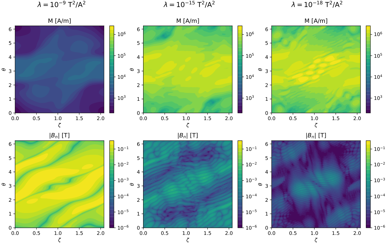
At large , the trade-off curve extends infinitely far to the left. In this limit, , so the solution is . With no permanent magnets, has a nonzero value associated with the fixed field . At the other limit of small , arbitrarily small values of and arbitrarily large values of are obtained. (The curve eventually bends to the right but very large numerical resolution is required in this region, so only the converged section is displayed.) In this limit, the component of normal to the target plasma surface is made arbitrarily small due to extremely large values of . The regularization vanishes in this limit, so very short-scale patterns in arise. A user must choose an intermediate value of that balances magnet complexity against physics properties of the plasma configuration.
| Run # | ||||
|---|---|---|---|---|
| 1 | 128 | 128 | 32 | 3 |
| 2 | 128 | 128 | 32 | 6 |
| 3 | 256 | 128 | 32 | 3 |
| 4 | 128 | 256 | 32 | 3 |
| 5 | 128 | 129 | 64 | 3 |
3.3 Fixed-point iteration
We now add the fixed-point iteration (7), considering the same 0.5 T NCSX geometry from the previous subsection. The iteration converges fastest when the number of degrees of freedom in is close to the number of degrees of freedom in each component of , i.e. when and . Otherwise the spatial dependence of and in (7) does not match. Therefore for this section we use the parameters of run 5 from table 1. We choose TA2. We also choose a target magnetization T MAm, achievable with rare-Earth magnets.
Figure 6 shows the convergence of the fixed-point iterations. It can be seen that the minimum and maximum of over both quickly converge to the target . Figure 6.b shows the difference in between successive iterates, measured by the maximum over and of . The difference converges to zero, demonstrating that a fixed point has been found.
Also shown in figure 6 are results when Anderson acceleration [19, 20] is applied to the iteration. In Anderson acceleration, a linear combination of the previous few iterates is used instead of only the previous iterate. The extra computational cost of the Anderson step compared to (7) is so small as to be negligible, and here it provides a modest acceleration in convergence.
The evolution of the spatial dependence of and is shown in figure 7. It can be seen that both and converge rapidly. By eye, is uniform and equal to by iteration 3, and changes to are hardly visible after iteration 1. The final result for the shape of the magnet region is displayed in figure 8.

It is not obvious that for any choice of initial , the iteration is stable and the fixed point obtained is the same. However it appears that a unique solution exists in practice, at least for the examples in this paper. The calculation of this section was repeated with various uniform initial meters. (Larger values are not permitted because the outer surface begins to self-intersect as crosses through zero.) The calculation was also repeated taking the initial to have a random variation in and within m. As shown in figure 9, differences between these differently-initialized calculations converged steadily towards zero as the iterations proceeded. This behavior is in contrast to the formulations in [14, 13] in which dependence on the initial condition was observed. The independence of REGCOIL_PM results from the initial condition is advantageous, since a user need not worry about how best to select the initial condition.
4 Verification for Halbach cylinders
A satisfying property of the mathematical formulation of section 2 is that it is consistent with the analytic solution for cylindrical multipole magnets (“Halbach cylinders”) described by Halbach [21]. A comparison with this analytic result also serves as a useful test of the numerical implementation of section 3.
4.1 Analytic solution
We first derive the analytic solution by a different method than in [21] to highlight the parallels with stellarator magnet optimization. We consider two concentric infinite cylinders, an inner one with radius analogous to the plasma surface, and an outer one with radius analogous to a thin magnet volume. This configuration can be imagined as a high-aspect-ratio limit of an axisymmetric system, so the angle around the cylinder is a poloidal angle. Let us try to arrange magnetic dipoles on the outer surface in order to create a normal magnetic field
| (12) |
on the plasma surface, where is a given integer. In other words, suppose there is a fixed normal field , and we wish to introduce dipoles to obtain . We will consider two possible arrangements of dipoles, shown in figure 10: first, dipoles of uniform magnitude but arbitrary direction, as in a REGCOIL_PM solution; and second, dipoles oriented normal to the outer surface but with arbitrary magnitude. This second case is considered because dipoles oriented normal to a surface have been considered in recent papers [12, 13]. We will show the magnetization magnitude in the first approach is half of the maximum magnetization in the second.
Outside of the region of dipoles, the magnetic field can be written for a scalar potential . The potential for a single point dipole is where
| (13) |
Here, is the magnetic moment, is the position vector of the dipole, and is the observation location. The gradient of (13) gives the expected field
| (14) |
We introduce cylindrical coordinates and Cartesian coordinates with the axis along the axis of the cylinder, and associated unit vectors . Again we use primes to indicate coordinates on the magnet surface, so the evaluation and source positions are
| (15) | ||||
Supposing the dipoles cover the surface with a uniform number density (units of 1area), then the total potential is
| (16) |
For the first of the two configurations, shown in figure 10.a, we consider dipoles
| (17) |
for some integer and constant so is uniform. The integral (16) for this case is evaluated in B, with the result
| (18) |
for . We will not need the field for . The magnetic field normal to the inner surface is then
| (19) |
Comparing this result to (12), we see the desired field is produced on the plasma surface if we choose and
| (20) |
Expression (19) for a thin layer of dipoles can be extended to a formula for a finite-thickness magnet with inner radius and outer radius by writing and integrating in over . The result is
| (21) |
This result is equivalent to the radial component of (21a) in [21], Halbach’s multipole, noting the following substitutions: , , , and . Equivalently, the magnetization required to produce the field (12) is
| (22) |
Since this dipole configuration produces the desired (12) exactly, then when it is added to the aforementioned equal and opposite fixed field one obtains . Therefore this dipole configuration is a solution of the RECGOIL_PM least-squares step in the limit of small . Furthermore, since is uniform, this configuration is a fixed point of the Picard iteration. Therefore this configuration is a fixed point of the overall REGCOIL_PM algorithm.
We can compare this first configuration of dipoles with the second configuration, in which the dipole directions are constrained to lie in the direction normal to the surfaces, now allowing to vary with . This second configuration is illustrated in figure 10.b. We assume the magnitude of the dipoles is for some constant , so
| (23) |
This expression is substituted into (16), and after evaluating the integrals as shown in B, one finds for
| (24) |
for . We will not need the field for . The field normal to the plasma surface is then
| (25) |
Comparing this expression to (12) it can be seen that the desired field on the plasma surface is produced if the maximum dipole magnitude is
| (26) |
The fact that the dipole arrangements (17) and (23) can both produce the same field (12) on the plasma reflects the significant freedom available in choosing the magnets for a given stellarator. Comparing (26) to (20), we see that the required maximum dipole magnitude is twice as large when the dipoles are constrained to lie normal to the magnet surface compared to the arbitrary-orientation case.
4.2 Numerical solution
We now compare the analytic result (22) to numerical calculations with REGCOIL_PM. Since the code is written for toroidal geometry rather than cylindrical geometry, we choose a very large but finite aspect ratio, with major radius 30 m, m, m. We also choose T and, initially, . For this section we neglect the Picard iteration to focus on the behavior of the regularized least-squares problem, fixing mm. We use the following resolution parameters: 96 grid points poloidally, 512 grid points toroidally, 24 Fourier modes poloidally, and 2 grid points radially.
First, the behavior of the regularized least-squares solution is examined as the regularization parameter is varied. As shown in figure (11), as is decreased below T2/A2, the normal field error can be made arbitrarily small, indicating the permanent magnets exactly produce the desired field. This regime corresponds to the vertical part of the Pareto curve in figure 11.a. For above this threshold value, the problem becomes over-regularized, with the regularization term forcing the magnetization to be very small such that the dipoles do not significantly cancel the fixed field. This regime corresponds to the horizontal part of the Pareto curve in figure 11.a. For the rest of this section we focus on values of below the threshold, for which the magnet distribution and are insensitive to , and is very small.
Next, figures 12.a-b show a comparison of the magnetization computed by REGCOIL_PM to the analytic result (22), as or are varied. In both figures, error bars are given for the numerical results, displaying standard deviation of as is varied over and is varied over T2/A2. The error bars are barely visible, indicating that is found to be uniform and independent of the regularization, as it should be. Extremely close agreement is found between the analytic and numerical results.
Finally, figure 13 displays a 3D rendering of the numerical solution for , m. The magnetization vector is displayed with black arrows. It can be seen that the REGCOIL_PM procedure has indeed “discovered” the Halbach solution of figure 10.a.

5 NCSX example
We now further develop and analyze the NCSX example. In the following subsections, we demonstrate the ability to remove magnet in regions to make room for ports, free-boundary equilibria using the permanent magnets, and the difficult in raising the field magnitude. Finally we present a comparison to the different algorithm of ref [14].
5.1 Ports
It is infeasible to surround the plasma completely with permanent magnets, since access is required for heating, diagnostics, and maintenance. We therefore now show how regions of the permanent magnets can be removed for ports. The feasibility of including ports in the 0.5 T NCSX configuration was examined previously in [14, 12, 13].
Port regions are selected in REGCOIL_PM by increasing the local value of the weight in (5). For the example here we choose the following function for the weight:
| (27) | ||||
This function is appropriately periodic in the two angles, and the sum over allows multiple ports to be included. Port is centered at and , while the extent of the ports in and is controlled by and . The parameter controls the sharpness of the transition from to . In the example here, we choose port 1 to have , , , , , and . Additional ports are included with the same parameters but at stellator-symmetric and -symmetric locations. These values are chosen to align the ports with the regions of lowest magnet thickness, which are at the outboard side. The resulting function is shown in figure 14.
The REGCOIL_PM solution with ports is displayed in figures 15 and 16. The same regularization parameter is used as in section 3.3, TA2. It can be seen that the change to the magnet geometry is minor. A slight thickening of the magnet volume around the edge of the port is apparent. When ports are included, the volume of permanent magnets increases only slightly, from 2.012 m3 to 2.025 m3. The maximum also increases only slightly, from 0.00299 T without ports to 0.00303 T with ports. These results indicate it is likely that ports can be included in permanent magnet stellarators, at least in some locations.
A three-dimensional rendering of the REGCOIL_PM solution with ports is shown in figure 17. In the magnetization region, arrows with uniform length are drawn everywhere except the ports to show the direction of .


5.2 Free-boundary equilibria
To evaluate whether a magnet design is adequate, it is necessary to compute the resulting free-boundary plasma configuration. To this end, figure 18 shows a comparison of the original c09r00 target configuration with the configurations achieved with permanent magnets. To compute the latter, our REGCOIL_PM implementation saves an MGRID file that is used as input to free-boundary VMEC [22, 23]. REGCOIL_PM results are shown both with and without ports, corresponding to figures 8 and 16. Panels (a)-(b) of figure 18 show that the magnetic axis and flux surface shapes achieved are very close to those of the target configuration. Panel (c) shows that the rotational transform profile is reproduced accurately as well. Differences between the REGCOIL_PM results with and without ports are barely perceptible, indicating again that it should be possible to include ports in the design. More detailed analysis must be done to assess whether the small differences in flux surface shape have a meaningful effect on physics properties. Nonetheless, these preliminary results support the idea that producing the 0.5 T NCSX configuration with permanent magnets is feasible.
5.3 Higher field
Since the NCSX example developed in previous sections has a relatively weak magnetic field T, a natural question is whether the field magnitude can be increased. Here we examine the feasibility of doubling the field to 1 Tesla. In the approximation that the field produced by a permanent magnet is proportional to its thickness (figure 1), doubling would require a doubling of the magnet thickness. In fact the thickness must be more than doubled, since the new magnet that is introduced compared to the 0.5 Tesla case is farther from the plasma and so has less effect. Figure 19 shows the REGCOIL_PM solution for the 1 Tesla case with no ports, and a comparison to figure 8 makes clear that a significant increase in magnet thickness is indeed required. The magnetization volume for the 0.5 Tesla case is 2.0 m3, compared to 4.9 m3 for the 1 Tesla case. The magnet thickness for the 1 Tesla case is sufficiently large that the coordinate system in (3) becomes singular, with crossing zero. This issue is specific to the coordinate system we have chosen in regions where the inner surface is concave, and does not necessarily mean a 1 Tesla solution is impossible. However the significant volume occupied by the magnets in figure 19 suggests that a Tesla NCSX with the existing toroidal field (TF) coils and permanent magnets is likely infeasible. It may well be possible to obtain 1 Telsa solutions if the TF coils were shifted or rotated, or if a different plasma geometry is chosen.
5.4 Benchmark with FAMUS
It is interesting to compare the results of REGCOIL_PM to the topology optimization method described in [14]. The latter approach is implemented in the code FAMUS. In topology optimization, the presence or absence of a magnet at a given location is represented by a continuous variable , and optimization is used to penalize intermediate values in the range so or at most locations. The FAMUS and REGCOIL_PM approaches are expected to each have advantages and disadvantages. The potential advantages of REGCOIL_PM have already been described. Topology optimization is more flexible with respect to the magnet geometry, with no restriction that all magnets have one fixed surface specified by the user.
We carry out a comparison between the two codes for the 0.5 T NCSX case with no ports or plasma current. We first obtain a FAMUS solution, considering dipoles allowed to lie within 14 cm of the NCSX vacuum vessel in the direction away from the plasma. The grid of allowed dipole locations has a resolution of 14 points radially, 64 points in , and 384 points in (considering all field periods). The level of regularization in FAMUS is set by hand to achieve a plausible solution, with T2 m2. Then in REGCOIL_PM is adjusted to match this value of , with the result T A2. Both codes achieve the same target magnetization Am2. An effective volume of the permanent magnet region can be defined in FAMUS by where are the discrete dipole moments; the result for this case is 2.32 m3. The permanent magnet volume of the REGCOIL_PM solution is slightly lower, 1.96 m3.
The results of the two codes are shown in figure 20. It can be seen that or 1 nearly everywhere in the FAMUS solution. For both codes, black arrows display the magnetization vector’s projection into the -plane. While is exactly uniform in the REGCOIL_PM solution and very nearly uniform in the FAMUS solution, the arrow lengths vary since a component may be present. In panels (a)-(c), the vectors are shown for 4 of the 14 radial grid locations in FAMUS. In REGCOIL_PM, where there is no radial variation, only a single arrow is shown. The dipole locations in FAMUS are shifted from the symmetry planes by half of the grid spacing (i.e. by radians), so the figures show the nearest planes of dipoles to the given . There are many similarities between the solutions from the two codes. Both codes yield a thicker magnet layer on the small- side of the plasma. In these thick regions, the direction of the magnetization is very similar between the two codes. At the large- side, the REGCOIL_PM solution has a thin magnet layer, whereas FAMUS eliminates the magnets in many of these regions. These two different magnet configurations both produce a small field error , demonstrating again that there is significant flexibility in the magnet design.
6 Conclusions
In summary, we have demonstrated an algorithm for computing an arrangement of permanent magnets outside of a target volume that produces a desired spatially-dependent magnetic field inside the volume. While the algorithm is applied here to stellarators, the method could be used for other applications as well. The method here results in a binary magnetization magnitude: at every point is either zero or equal to a target value . This feature is advantageous since any volume occupied by magnetization of less than the maximum commercially available magnitude is an inefficient use of space. The method also does not place constraints on the direction of , meaning that Halbach solutions with rotating are obtained automatically. While we have not rigorously proved stability or existence of a unique fixed point, the method appears to give a unique result independent of the initial guess, meaning users need not worry about how to choose a good initial condition.
In this work for expediency we have considered the case of magnets in a domain with smooth boundary and with smoothly varying . This approximation is likely inaccurate for a serious experimental design. However it appears straightforward to extend the REGCOIL_PM algorithm to a more realistic case of discrete magnet blocks with a uniform direction of in each block. Each block would be parameterized with a thickness parameter . The linear-least-squares solve would have three degrees of freedom per block, one for each coordinate of the block’s vector. The parameter of each block could be updated by applying the same fixed-point iteration used here to each block. This idea will be explored in future work.
Even without this extension to discrete magnet blocks, REGCOIL_PM could be valuable as part of optimization of the plasma shape, i.e. the first stage in the standard two-stage stellarator design. At each iteration of the plasma optimization, REGCOIL_PM could be called, and the resulting magnet thickness could be penalized in the objective function along with other physics quantities. One could thereby find plasma configurations that can be produced with a relatively low volume of permanent magnets. Inside this optimization, robustness and speed of a code are more important than detailed modeling of all engineering factors, and so the ‘smooth’ REGCOIL_PM of the present paper would be sufficient and well suited. For this application the number of fixed-point iterations (eq (7)) could be very small, perhaps one, since the magnet thickness need not be precise. Or, the fixed-point iteration could be avoided entirely, and rather the peak magnitude from the linear-least-squares solution with uniform could be penalized.
Appendix A Jacobian
Appendix B Integrals for section 4
Here we derive expressions (18) and (24). We start by inserting (17) (for uniform-magnitude dipoles) or (23) (for dipoles normal to the magnet surface) into (16). The results are
| (31) |
and
| (32) |
respectively. The integrals are evaluated using for . Changing the remaining integration variable to and using an angle-sum trigonometric identity, one finds
| (33) |
with
| (34) | ||||
and
| (35) |
The contributions from terms , , and all vanish. The remaining integrals can be evaluated using
| (36) | ||||
References
References
- [1] R Turner. Gradient coil design: a review of methods. Magnetic Resonance Imaging, 11:903, 1993.
- [2] M Poole and R Botwell. Novel gradient coils designed using a boundary element method. Concepts in Magnetic Resonance B, 31B:162, 2007.
- [3] S S Hidalgo-Tobon. Theory of gradient coil design methods for magnetic resonance imaging. Concepts in Magnetic Resonance A, 36A:223, 2010.
- [4] L Rossi and E Todesco. Electromagnetic design of superconducting quadrupoles. Phys. Rev. ST Accel. Beams, 9:102401, 2006.
- [5] S. Russenschuck. Field Computation for Accelerator Magnets: Analytical and Numerical Methods for Electromagnetic Design and Optimization. Wiley, 2011.
- [6] P Merkel. Solution of stellarator boundary value problems with external currents. Nucl. Fusion, 27:867, 1987.
- [7] M Drevlak. Automated optimization of stellarator coils. Fusion Tech., 33:106, 1998.
- [8] D J Strickler, L A Berry, and S P Hirshman. Designing coils for compact stellarators. Fusion Sci. Tech., 41:107, 2001.
- [9] M Landreman. An improved current potential method for fast computation of stellarator coil shapes. Nucl. Fusion, 57:046003, 2017.
- [10] C Zhu, S H Hudson, Y Song, and Y Wan. New method to design stellarator coils without the winding surface. Nucl. Fusion, 58:016008, 2018.
- [11] P Helander, M Drevlak, M Zarnstorff, and S C Cowley. Stellarators with permanent magnets. Phys. Rev. Lett., 124:095001, 2020.
- [12] C Zhu, M Zarnstorff, D Gates, and A Brooks. Designing stellarators using perpendicular permanent magnets. Nucl. Fusion, 60:076106, 2020.
- [13] K Hammond, C Zhu, T Brown, K Corrigan, D A Gates, and M Sibilia. Geometric concepts for stellarator permanent magnet arrays. Nucl. Fusion, 60:106010, 2020.
- [14] C Zhu, K Hammond, T Brown, D, M Zarnstorff, K Corrigan, M Sibilia, and E Feibush. Topology optimization of permanent magnets for stellarators. Nucl. Fusion, 60:106002, 2020.
- [15] N Pomphrey, L Berry, A Boozer, A Brooks, R E Hatcher, S P Hirshman, L-P Ku, W H Miner, H E Mynick, W Reiersen, D J Strickler, and P M Valanju. Innovations in compact stellarator coil design. Nucl. Fusion, 41:339, 2001.
- [16] M Landreman. Dataset on Zenodo, http://doi.org/10.5281/zenodo.4029009. 2020.
- [17] M Landreman. Dataset on Zenodo, http://doi.org/10.5281/zenodo.4028933. 2020.
- [18] M Drevlak, C D Beidler, J Geiger, P Helander, and Y Turkin. Optimisation of stellarator equilibria with ROSE. Nucl. Fusion, 59:016010, 2019.
- [19] D G Anderson. Iterative procedures for nonlinear integral equations. J. Assoc. Comput. Mach., 12:547, 1965.
- [20] T Sánchez-Vizuet and M E Solano. A hybridizable discontinuous Galerkin solver for the Grad–Shafranov equation. Comp. Phys. Comm., 235:120, 2019.
- [21] K Halbach. Design of permanent multipole magnets with oriented rare Earth cobalt material. Nucl. Instrum. Meth., 169:1, 1980.
- [22] S P Hirshman and J C Whitson. Steepest-descent moment method for three-dimensional magnetohydrodynamic equilibria. Phys. Fluids, 26:3553, 1983.
- [23] S P Hirshman, W I van Rij, and P Merkel. Three-dimensional free boundary calculations using a spectral Green’s function method. Comp. Phys. Comm., 43:143, 1986.
- [24] M Landreman and E J Paul. Computing local sensitivity and tolerances for stellarator physics properties using shape gradients. Nucl. Fusion, 58:076023, 2018.