Regularization for the inversion of Fibre Bragg Grating spectra
Abstract
Fibre Bragg Gratings have become widespread measurement devices in engineering and other fields of application. In all but a few cases, the relation between cause and effect is simplified to a proportional model. However, at its mathematical core lies a nonlinear inverse problem which appears not to have received much attention in the literature. In this paper, we present this core problem to the mathematical community and provide a first report on opportunities and limitations of a regularization approach. In particular, we show that difficulties arise from non-uniqueness and the absence of established parameter selection rules for nonlinear inverse problems with multiple regularization parameters. Nevertheless, the paper takes a first step toward extracting more information from a single FBG measurement.
1 Introduction
Since their first demonstration in the late 1970s [4], fibre Bragg gratings (FBGs) have become a widely used technology for measuring physical quantities such as strain, temperature, or concentration. They also have a broad and important role in other settings, and we refer to [13] for an overview. Our intended application is the measurement of strain in fibre-reinforced polymers, but in this work we focus on a fundamental inverse problem common to all applications. Technologically, an FBG consists of a segment in an optical fibre in which a periodic variation of the refractive index has been inscribed. Some common FBG inscription patterns are shown in Figure 1.

Depending on the specific grating pattern, certain wavelengths of light are reflected at the grating as they propagate through the fibre. Hence, when the fibre carrying an FBG is probed with light, usually emanating from a tunable laser, a narrow band of wavelengths is reflected. The intensity of the reflected light (its spectrum) serves as the measured data, and the fundamental task lies in recovering the refractive index distribution inside the grating zone from the observed spectrum. The quantity to be measured in the specific application is then inferred from the reconstructed refractive index distribution. A schematic view of an FBG and its measurements is shown in Figure 2.

In the majority of applications the spectrum consists of a single peak at a specific wavelength. Temperature changes or applied strain cause the peak to move to another wavelength. The difference between the old and new peak wavelengths allows a quantification of the applied strain (or other quantity of interest). It is well known that under certain conditions the single peak can broaden and even split into two (or even more) separate peaks. The simple formula for the peak deviation then becomes increasingly uninformative and inaccurate, and existing measurement devices then abort the measurement process or yield unrealistic data. Hence, peak deformation is widely regarded as an undesired phenomenon. However, such a multi-peak spectrum contains much more information besides the peak location. The aim of this work is to extend the analysis of FBG signals from mainly peak-focused considerations to the full spectrum, and to extract as much information from the spectrum as appears possible. We emphasize that this paper is written as an introduction of the problem to the inverse problems community and reports first results, but also leaves some open problems for future work.
The remainder of the paper is organized as follows. In Section 2 we introduce basic FBG concepts as well as the model for the FBG refractive index distribution. In Section 3 we sketch the derivation of the forward model to provide the physical background and discuss the implementation. In Section 4 we provide a first result on the uniqueness of FBG spectra. Our regularization approach is presented in Section 5. In Section 6 we apply the theoretical results to experimental data.
2 Fibre Bragg Gratings
In the following we sketch the most important aspects of the physics underlying FBGs. Due to the complex nature of the topic, many details are omitted, and for these we refer to, for example, the monographs [7, 6, 5], or the survey papers [13, 8] and references therein.
Optical waveguides. As the name suggests, the base for an FBG is an optical fibre. Such fibres consist of three concentric layers: a relatively thin core with refractive index in which (most of) the light is guided, a comparatively thick cladding with refractive index , and a thin coating to protect the inner layers; see Figure 2. Next we note that light is guided in a specific way in a fibre. Consider a plane wave travelling in the fibre at an incident angle . Firstly, only incident angles can be guided, as otherwise the light is not reflected back into the core at the core-cladding interface, but rather refracted into the cladding. Secondly, even below this threshold, only a discrete set of inclination angles result in a propagating wave, as otherwise the wavefronts become out of phase and the wave breaks down. The superposition of the travelling wavefronts with constant phase in turn produces a standing wave inside the fibre. This standing wave is called a guided mode. If the core refractive index and the cladding refractive index are sufficiently close, then only a single mode is guided in the fibre. We will only consider this case in the following. We also mention that some modes can also be guided in the cladding, but this will not be pursued in this paper.
Remark 1.
Another important effect one may encounter in measurements is birefringence. This significantly adds to the complexity of the reconstruction, and in order to keep the presentation simple we ignore this effect in this paper. Birefringence results from the fact that each guided mode consists of two polarization states, which normally do not interact with each other. Mathematically speaking, the electric fields are orthogonal. Some external causes, most prominently a deformation of the fibre core from an initially circular cross section to an elliptical one, lead to differing propagation properties between the two polarization states. Orthogonality is lost, and the two polarization states can exchange energy. This is one of the main causes for the splitting of a the single peaks usually observed in FBGs. For more details see, e.g., [2].
The wavelength-dependent propagation constant describes how phase and amplitude vary along the propagation direction. For a guided mode with incident angle travelling in a medium of refractive index , it is given by
The effective refraction index describes the propagation in the fibre direction. Because in a fibre is small (as ), and are often used (almost) interchangeably [8]. One might say that is simply the average refraction index in the grating section of the fibre.
Bragg gratings are reflection gratings. The effect of a planar wave incident on a grating of (period-)length at an angle in a medium with refractive index can be described by the equation
| (1) |
where is the refractive index of the medium after refraction, the “outgoing” angle, the refraction order, and the wavelength [3]. For Bragg gratings, the dominant refraction is first order () refraction of a mode under its negative incident angle, i.e., . For a fixed mode with , (1) can be written in the form of the well-known Bragg condition for the design wavelength ,
| (2) |
This is the basic relation which suffices as a basis for the measurement of strain, temperature, etc., in many applications. Specifically, a change in these quantities results in a shift of the peak wavelength . For example, uniaxial strain in fibre direction at constant temperature yields a peak shift of
see, e.g., [2]. Using some engineering mechanics, one can reformulate this to the relation
| (3) |
i.e., the measured shift in peak wavelength relative to the original peak wavelength is proportional ( depends on material parameters) to the longitudinal strain. This is a highly simplified model. The measurement devices (interrogators) measure the intensity of the light reflected by the FBG over several wavelengths, the spectrum.
However, (2) and the occurring quantities are only a rough characterization of the FBG. We now turn to a more detailed description. To this end, note that FBGs are usually inscribed into the fibre by phase-masking or via the interference of two UV-light rays (see, e.g., [13, 7]). Although the fibre and thus the Bragg grating are three-dimensional objects, the refractive index distribution is modelled as one-dimensional, varying only along the longitudinal coordinate. Specifically, let the fibre section containing the FBG be of length . Then the common model to describe the grating structure is
| (4) |
where is the longitudinal coordinate. The functions and , which influence the magnitude of the refractive index perturbations, are sometimes connected via the fringe visibility such that , but we employ the slightly more general setting here. In this paper the base period length of the grating is denoted by , and all deviations from this basic period are encoded in the function . The functions and allow to describe complex grating structures including common FBG designs as those shown in Figure 1.
The refractive index in the fibre core is then given by
| (5) |
3 Forward Model
The forward model can be derived from Maxwell’s equations combined with coupled mode theory. The complete derivation is rather technical and does not provide much insight into the problem from a mathematical point of view. We therefore only sketch the most important steps. For an exhaustive derivation we refer to [7].
From Maxwell’s equations one derives the wave equation
| (6) |
relating the electric field and the polarization inside the fibre. Here are vacuum permeability and permittivity, respectively. Using the weakly guiding approximation (assuming the electric field has only transversal components), one can drop the term . The electric field and the polarization are further related via , where the relative permittivity of the medium (here: the fibre core). In non-magnetic materials such as optical fibres, the permittivity is connected to the refractive index via . In case of perturbations, we write
| (7) |
and
| (8) |
Typically the term is neglected, as it is generally at least two orders of magnitude smaller than . We thus have
| (9) |
and the polarization can be written as
| (10) |
Inserting this into (6) yields, after some rearrangement,
| (11) |
Next, one makes an ansatz for the electric field. For the single mode fibres we consider here, we set
| (12) |
Here, and are the (complex valued) transversal electric fields of the forward () and backward () propagating waves which propagate along the fibre with amplitude and , and with propagation constants and (notice the different signs of the propagation constants indicate reversed direction), respectively. We insert (12) into (11), which yields after some calculation the relation
| (13) |
In particular, we have employed the slowly varying envelope approximation, i.e., , which allows to neglect second-order derivatives. Next we split (3) into two equations by multiplying with the complex conjugate transversal fields and , and integrating over the fibre cross section (--plane). We will only purse the first path further, the latter follows analogously. Note that in the absence of refractive index perturbations the transversal fields are orthonormal, , and analogously for and exchanged. Due to conservation of energy (the frequency of the generated wave must not change), we can divide (3) by and, all together, obtain
| (14) |
where we insert the grating refractive index distribution (1), in which we replace for brevity. This yields
| (15) | ||||
| (16) | ||||
| (17) |
From this formulation, we continue with the last crucial step, the so called phase-matching. The principle behind this is that modes can only exchange energy if they are in phase for a sufficiently long way. Comparing the phases in (15) and (16), we see that and the -component of are always in phase , while this is never the case for and the -component of due to the modulation . On the other hand, comparing the phases in (15) and (17), we see that the -term of is never in phase with , while this may (partially) be the case for the -term. To describe the latter properly, one introduces the phase-synchronous factor , such that a continuous transfer of energy occurs for . We define the phase mismatch
For the single mode fibres under consideration, the remaining integrals are easily evaluated and yield the coupling coefficients
| (18) |
and the -coupling coefficient
| (19) |
Now we can write Eqs. (15)-(17) in a more compact way as
| (20) |
Repeating the same steps for the second branch of (3), we obtain
| (21) |
Finally, we substitute
| (22) |
(where is short for reference, or the light going into the FBG, and is the signal, or measured, reflected light), and adopt the common notation
| (23) |
with the convention (note: for single-mode fibres )
| (24) |
from (2) and (for a single-mode fibre)
This finally yields the well-known system of coupled ordinary differential equations
| (25) |
for in the grating zone, i.e., , of an FBG of length . To find a solution, one typically imposes the boundary conditions (light enters the FBG with full intensity) and (no light is reflected beyond the FBG).
Finally, the measured data corresponds to the (relative) intensity of the reflected light,
| (26) |
Note that the coupled system (3) has complex-valued coefficients, but the measured data consists only of intensities. The phase information is lost. Therefore, the task of recovering the functions , and , which are hidden in the coefficients and , from the data , is a phase retrieval problem with a nonlinear forward operator.
Since one is only interested in the reflected spectrum, the system of equations (3) can be rewritten as a Ricatti-type differential equation by making the substitution . This yields
| (27) |
and . In case of a homogeneous grating, i.e., , , and such that and are also constant for fixed , then (3) (and (27), respectively) have an analytic solution. Defining
| (28) |
one can show that
| (29) |
In practice, integrating (3) or (27) numerically is rather time consuming. Instead, one commonly uses the transfer matrix approach [8]. The idea behind this approach is to divide the Bragg grating of length in subelements of uniform length that are sufficiently long (). For each subelement , , one has
| (30) |
where are the amplitudes of ingoing and reflected spectrum before the subelement, the amplitudes after the subelement, and the transfer matrix is given by
| (31) |
Above, , and are the coefficients (23) and (19) averaged over the subelement . Numerically, are evaluated as where is the central coordinate of the subelement .
One then links all subelements by multiplying their transfer matrices such that with
| (32) |
one has
| (33) |
Together with the boundary conditions ( and ) one finally obtains
| (34) |
for the reflection intensity.
To sum up, the forward operator
| (35) |
maps three (potentially) unknown functions to the spectrum. To discretize the problem, we use discretization of the unknowns implied by the transfer matrix formulation. The spectrum is discretized by pointwise evaluation, which in practice is determined by the measurement device. Note that the rather coarse discretization here reduces the degrees of freedom significantly, and acts as a first important regularization. Even more, fine discretization of the unknown functions over the entire grating length is infeasible. In order to fully resolve as in (5), a high spatial resolution is needed to avoid aliasing effects. For example, a typical period length in (4) would require roughly 4000 discretization points per millimetre FBG-length to satisfy the Nyquist sampling criterion, if one wanted to discretize (4) in a straightforward way. As a comparison, our experimental setup yields about 10 significant points in the spectrum.
4 Uniqueness
An important question for the inversion of an FBG-spectrum is its uniqueness: Is a spectrum uniquely determined by the three functions , or can multiple configurations produce the same data? We have only found one partial answer in the literature. In [12] it was mentioned that the period distribution (corresponding in our notation to is reversible without affecting the data, i.e., one can not discern between and . This is true in their setting, but not in general. Except for this reversal, the authors claim uniqueness with respect to the distribution of over the FBG, and attribute it to the fact that the matrix multiplication in the transfer matrix formulation in (32), (34) is not commutative. However, this only guarantees that the transfer matrix does not introduce additional non-uniqueness. The actual source of non-uniqueness lies in the physical model. What holds is the main argument of [12] that the FBG can not distinguish between light propagating in forward and backward direction. The following theorem explains this mathematically and gives an extended result on the uniqueness of the FBG spectra. We stress that we do not claim completeness of the list.
Theorem 4.1.
Let be a reflected FBG spectrum. Then the following ambiguities hold:
- (a)
for all ,
- (b)
,
- (c)
if , ,
- (d)
if .
Proof.
Since the coupled system (3) only uses , any constant in disappears, hence a) holds. Because of (19), and have the same sign, which is lost due to taking the absolute value in (26). This is easily seen from (27). Multiplying the equation by , we can write
which yields the identical ODE for . The sign, however, is lost in the intensity (34). Note that such a trivial ambiguity is common for nonlinear phase retrieval problems, see, e.g., [1].
For c) and d), we use the reversibility of the FBG as noted in [12]. Take the coupled system (3), exchange the roles of and , and set , i.e., and . Then the system can be written as
| (36) |
which coincides with (3) if and . Because only the derivative of enters , this yields the requirement , which holds if . ∎
It is also worth mentioning that the non-uniqueness for FBGs is already inherent in the Bragg-wavelength (2), . If neither nor are known, there are infinitely many pairs that produce the same . Related to this, we deem it important to report a potential “pseudo non-uniqueness” of the spectra with respect to practical measurements. Namely, despite being different, some configurations of the unknowns may yield spectra that are only distinguishable in small differences that may easily get lost during the measuring or (forward) simulation process. To exemplify this, we simulate two spectra with two distinct peaks at wavelengths nm and nm. All parameters are identical, except that in one spectrum we set
whereas for the other spectrum we set
As shown in Figure 3, this yields spectra that visibly only differ in the low intensity regions away from the peaks. The maximal difference is smaller than , which as discussed in the experiments in Section 6, is already within the noise level.


We have shown that FBG spectra are, in general, not uniquely determined and that they may appear identical despite varying slightly. Therefore, when conducting experiments, it is advisable to employ as much asymmetry as possible in the positioning or the expected reaction of the FBG, as well as use precise measuring devices.
5 Regularization
In this section we present a regularization approach for several configurations of the potential unknowns. As explained in Section 3, the full problem consists of identifying three functions () from the measured spectrum . However, it is not always necessary to consider this general setting. Therefore, we begin with some special cases.
5.1 Homogeneous FBG
The most common FBG design is a homogeneous grating characterized by
Even then, in the authors’ experience, the manufacturers of the FBG are not always able to provide precise values for or . Therefore, in a first step, which can also be seen as a calibration for later test cases, we aim to recover the two parameters from the spectrum of a homogeneous FBG. An experimental validation is carried out in Section 6.
To find the unknown parameters, we calculate
| (37) |
The minimizer is calculated in MATLAB by way of the function lsqnonlin using the Levenberg-Marquardt algorithm. Due to the low dimensionality of the problem, no regularization is necessary. However, as usual for highly nonlinear problems, the initial guess may influence the quality of the reconstruction. Due to the simplicity of the setting it is fairly easy to find a good initial guess by hand, since the only two free parameters have distinct effects: moves the spectrum along the -axis and controls the intensity (height of the peak). An example of such a recovery is shown in Figure 4. While it is not too surprising that we obtain perfect recovery of the parameters given the simplistic setting, we would like to highlight that this is an important calibration step for the experiments in practice. Specifically, the calculated value of can be used to correct the position of the peak and thus potentially eliminates a source of error in the strain calculation via (3).

5.2 Tapered and Apodised FBGs
The need for regularization arises as soon as an inhomogeneous refractive index distribution is to be found, i.e., a combination of , or is to be recovered as functions resolved over the FBG length. In this section we consider and to be unknown, which can be interpreted as the determination of apodized and/or tapered FBGs (cf. Figure 1).
In our example we consider an apodized and tapered FBG of length with and
For the discretization we use the transfer matrix approach with subelements, corresponding to a resolution of . The data consists of measured points with a wavelength spacing of , which is of comparable size to the real data. To find the minimizer we again employ the lsqnonlin-function of MATLAB to calculate
i.e., we penalize the -norm
to stabilize the recovery, and we now have two regularization parameters and . Among several tested penalty functionals, this gave the most reliable results. An appropriate choice of and then yields a good approximation to the correct functions and , as can be seen in Figure 6. Hence, we have demonstrated that it is possible to extract information from the FBG that is far more detailed than the usual peak-evaluation. A crucial step and a centrepiece of future research is the automatization of the search of a suitable pair of regularization parameters . Currently we pick the regularization parameters by hand knowing the exact solutions, which is clearly not ideal. However, only few methods are documented in the literature for the simultaneous estimation of two regularization parameters, and none of them seem to work in our situation. One approach is a generalization of the L-curve method. In the classical setting with one regularization parameter, the L-curve was introduced in [9] and has become a popular heuristic parameter sekection rule. It features a --plot of residual versus the corresponding penalty value, which often attains roughly the shape of an L. It is then advised to choose the regularized solution corresponding to the corner of the L. The principle has been extended to two-parameter regularization in [10] and recently successfully applied in [22]. In this case one plots the triples of residual and the two penalty values, each on a logarithmic scale. As generalization of the corner of the L, one then picks the regularized solution corresponding to the point on the “L-surface” with highest curvature, typically to be found close to the origin. Unfortunately, this method appears to be unsuitable for the recovery of the FBG refractive index distribution, see Figure 5. While in principle every cross-section of the L-surface is L-shaped and thus the points of high curvature are easily found, a comparison with the plot of the total reconstruction error (see also Figure 5) reveals that the best approximate solutions are found somewhere in the large, flat plane corresponding to the smaller regularization parameters. This plane, however, also contains the highly oscillating, underregularized approximations, as well as some approximations where the regularization parameters are already too large. The residual carries no meaningful information about the reconstruction error, so that other methods have to be developed. This observation also renders discrepancy-based parameter selection rules infeasible. Since our experimental goal is to calculate strain within a body, our plan is to link the FBG inversion with a finite element model of the body, and to find suitable regularization parameters through linking the two approaches.


5.3 Chirped FBG
So far, we have not considered the FBG period modulation as an unknown. We turn to this case in this section, where for now we let the other parameters and be known. To the best of the authors’ knowledge, this is the only case for which an inversion of the entire FBG-spectrum has previously been attempted. Indeed, in [12] a genetic algorithm was presented that could approximate the local grating period sufficiently well. We remark that the authors of [12] used a slightly different encoding of local period changes than done in this paper. We also remark that genetic algorithms, and the closely related evolution-type algorithms have to be treated with utmost care when used to solve inverse problems, see the extensive study in [23] in another context of phase retrieval under a nonlinear forward operator,
In addition the calibration of chirped FBGs (cf. Figure 1), the determination of can be directly related to axial strain along the fibre direction. Specifically, one has
| (38) |
where is the axial strain and the strain-optic coefficient of the FBG [12, 11].
We remark that the the period modulation enters the governing ODE system (3) only via its derivative (cf. the parameter in (23)). Hence, we reconstruct the function and obtain itself via numerical integration using the trapezoidal rule.
As in the previous section a direct recovery approach without regularization fails, as highly oscillating functions produce almost identical spectra as the true reconstruction. To suppress this, we employ again a Tikhonov-type approach
| (39) |
and obtain by integration,
| (40) |
If the integration constant is determined, the strain can be calculated from (38) as
| (41) |
The determination of an integration constant typically relies on some additional information, which in general is not available in our setting. Fortunately, we observed a kind of self-calibration effect that can be used to find . Indeed, by default we obtain from (40) with . We then calculate the strain according to (41) for a range of , , and with this the norms as function of . This function has a single minimum whose location coincides with the desired integration constant, see Figure 7 for examples with noise-free and noisy data..


To present an example for this scenario we attempted to reproduce Example 3 from [12]. There the strain function over an FBG of length is defined as
| (42) |
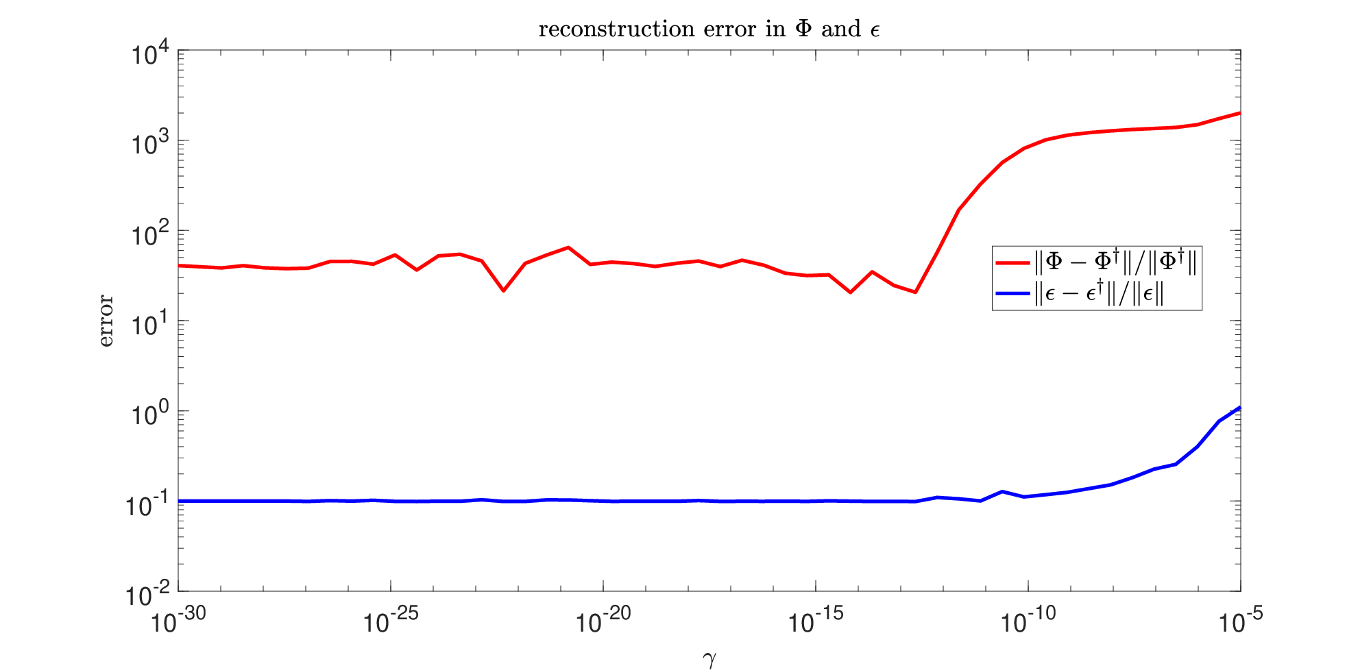
This strain function and its reconstruction with the method described above, as well as the simulated and recovered spectra, are shown in Figure 8 for noise-free data and in Figure 9 for noisy data. It is important to note that, comparing our spectral data with that in [12], it appears that our wavelength discretization is significantly coarser (we use an equidistant grid with spacing). On the other hand, we split the FBG into subgratings for the transfer matrix approach compared to in the original example. In particular, we obtain a spatial strain resolution of from only one FBG sensor. Similarly to the last section, we solve (39) for several values . In the absence of noise in the data, only a small amount of regularization is required. We obtain the best reconstruction for ; see Figure 8. We then repeat the experiment with 1% Gaussian noise added to the data. We still obtain good approximation of the unknown strain , see Figure 9 for . However, the approximations are sensitive with respect to the regularization parameter , and similar to the results in the previous section, it remains an open problem to find an automated way to determine an appropriate regularization parameter. Several established heuristic parameter selection rules have been tested, including the quasi-optimality criterion [20], the L-curve method [9], the heuristic discrepancy principle [21], and the simple L-curve [19]. The reason for this failure is likely the nonlinearity of the forward operator, as heuristic parameter selection rules are often developed for linear forward operators; as well as the previously noticed flatness of the residuals w.r.t. the regularization parameters. In Figure 10, we show residuals and reconstruction errors in phase and strain . It can be seen that without simulated data noise, the residuals fall continuously with decreasing until they reach a flat plateau. The minimal reconstruction error is to be found in the region of descending residuals. However, under noisy data this is no longer the case, as the residuals are almost unchanged for the range of regularization parameters shown. Also the reconstruction errors in and are flat, and it is difficult to locate the minima. Again, this indicates the need for adaptive parameter selection strategies, which remains a topic for future research.


 |
 |
 |
 |
In summary, we have demonstrated that it is possible to recover a strain distribution over the length of an FBG by minimizing a Tikhonov-type functional with a spatial resolution below 100m. The reconstruction quality depends strongly on the choice of the reconstruction parameter, and it remains an open problem to find a suitable rule for its selection.
6 Experiments
In this section we demonstrate the regularization approach with real measured data. We begin with the simplest test setting, a homogeneous deformation of the FBG. When using FBG sensors, a narrowband peak is a basic requirement for subsequent strain determination. A narrowband peak allows a main reflected wavelength to be determined. Various methods have been proposed in the literature for this purpose [15], e.g., by the centroid algorithm, the centre wavelength, a spline reconstruction or the full-width-at-half-maximum method (FWHM).
This reflected peak wavelength can now be determined at different points in time. Based on a change of the reflected wavelength, different physical quantities can be directly inferred. In our case this is the mechanical strain, which is obtained by solving for in (3), giving
| (43) |
This principle works well if the reflected peak is narrowbanded. In the literature two main effects are described where the reflected peak loses its narrowbanded form. These two effects, for which the peak widens or splits, are transversal and inhomogeneous loading of the sensor. Transversal loading (birefringence) is described in [17] and [18], see also Remark 1. This case is important for complex loading cases in complex components or reinforced materials, especially unidirectional reinforced materials. Currently this is not included in our model.
The second main effect is the inhomogeneous loading of a FBG sensor. This inhomogeneous case can occur in different situations. Foremost, the loading of a FBG sensor depends on the load case. Another source are geometric inhomogeneities, which also lead to inhomogeneous loading.
6.1 Experimental Setup and Specimen Design
In this paper we have intentionally created a geometric inhomogeneity to study the behaviour of FBG sensors and to test the inversion approach. Specifically, an aluminium bending beam was selected with linear-elastic material behaviour. The aluminium beam is loaded in a 4-point bending test, shown in Figure 12, as this produces an analytically well identifiable stressing in the region between the inner bearings, where the shear force is zero and the bending moment is constant.
In order to investigate the required magnitude of the inhomogeneity for producing an effect on the reflected peak, different specimens were produced, which are displayed in Figure 11. Different notches were manufactured in the aluminium beams. The geometry of these notches was determined by finite element simulation in Ansys. The notches were designed in such a way as to produce a specific characteristic of the strain along the FBG measuring length. This resulted in three variants of the test specimen. The first specimen shows a small strain gradient. The second specimen generates a medium strain gradient at the eccentric sensor of 30 % strain difference over the sensor length. A large strain gradient is produced by the third specimen, which has a strain difference at the eccentric sensor of 70 % over the sensor length.


The left panel of Figure 12 shows the experimental setup of the four-point bending test. In this experiment, a 100 kN ZwickRoell® testing machine is used. Besides a force controlled introduction of a preload, the loading is applied displacement controlled. Thereby, the force is measured by a 5 kN load cell. The displacement produces an approximated averaged strain of 2000 on the surface of the specimen. For this purpose, the punch is pressed onto a carriage, which introduces the force into the specimen via two mounted rolls (inner bearings). The outer rolls represent the outer bearings and are also rotatable. This means that no lateral force is generated. The produced, mean strain is measured by the electrical strain gauge with the MGCplus CP22 measurement system from HBM with catman AP V3.5.1.48.
Three different sensors are applied on each specimen as depicted on the right image of Figure 12. An electrical strain gauge is installed centrally above the notch and centrally at beam depth and serves as a reference sensor. The strain gauge we use, is a sensor 1-LY13-3/250 from HBM. Furthermore, two fibre Bragg grating sensors are applied. TOne edge of the so-called eccentric sensor aligns to the centre of the notch. The second, centric, sensor is centred above the notch. In this case draw tower gratings (DTG®) from FBGS with a sensor length of 8 mm were used. The FBG signal is measured by the FBGscan 800 from FBGS with the software program IllumiSense V.2.3.5.
Echoing the remark at the end of Section 4, our currently available measurement setup is not well suited to determine the complex loading configurations in the experiments we carried out. We know from the manufacturer that the employed FBGs are homogeneous ( , , ) with a length of 8mm. Other parameters such as , or the precise value of are not provided. Furthermore, the obtained spectra have a poor wavelength resolution of approximately 168nm, which alone is not enough for a precise characterization of the peak for the FBG without loading, since the FWHM of the peak is about 450nm. (In other words, the measured maximum spectrum may deviate from the correct peak due to the coarse discretization.) Finally, the spectra are not scaled according to the theory (with values up to around 80 for the intensity, which should reach 1 at maximum) and exhibit some background noise at an intensity of approximately 10 for which we have no explanation and which is not consistent with the forward model. An example of a measured spectrum is shown in Figure 13. We also show the rescaled spectrum which we use as input for the reconstruction algorithm: We take , divide by 100, subtract its minimum, and divide by the estimated peak value. To estimate the peak, we make a fit of the modified data to a Gaussian curve to find , and , and set . The rescaled data and an example of a homogeneous fit using the approach of Section 5.1 is also shown in Figure 13, which yields values for and . In order to obtain this, the remaining unknowns are mostly guessed. We find the peak wavelength of the unperturbed FBG and set which is a typical value. This yields . Despite the many inaccuracies, we show in the following that even from this “worst-case” data significant information about the FBG loading can be extracted.
Remark 2.
One can use the mentioned Gaussian fit directly to assess the shift of the peak in a homogeneous setting, since yields the peak wavelength. We demonstrate later that this approach appears to be slightly better than the evaluation of the software built into the interrogator.


6.2 Analysis of Experimental Data: Homogeneous Beam
In our first experiment we test the homogeneous setting, with the regularization as discussed in Section 5.1. While this is not the intended application of our method, it serves to demonstrate that the concept works, in particular with respect to the provided data. The results for the centric sensor are shown in Figure 14, they are similar for the eccentric sensor. We compare four evaluations of the strain: the strain gauge reading, the strain obtained directly from the interrogator, the strain calculated by a Gaussian peak fit (cf. Remark 2), and the strain calculated from the peak shift through the reconstruction of . All curves are close together and only differ in details. In the zoomed-in image, we see that the original data is not strictly linear as it appears superimposed with a sinusoidal wave of small amplitude. The Gaussian peak estimate is able to remove most of this sinusoidal wave and hence may be more accurate. The reconstructed curve is, arguably on average, closer to the strain gauge reading, but displays a distinct periodic staircasing effect. After several experiments, we attribute this purely to the insufficient data quality. Because the wavelength resolution is too coarse, there is an inherent sampling aliasing in the measurement process. We were able to recreate this in simulations with coarsely sampled spectra. Nevertheless, the resulting strain yields the lowest residuals to the measured data. Hence, we conclude that the algorithm itself works as intended.


6.3 Analysis of Experimental Data: Medium Strain Gradient
In this experiment we simulate a slight inhomogeneity in the strain applied to the FBG caused by an inserted notch. The notch produces a stress concentration which leads to an inhomogeneous deformation state. As seen in Figure 15, the eccentric sensor still sees an (almost) homogeneous loading, and the spectra only show a slight loss in peak height. The centric sensor, on the other hand, displays spectra that are considerably wider and of lower peak intensity for larger applied strain values. This means the homogeneous model becomes inaccurate. To illustrate this, we show in Figure 16 the strain reconstruction obtained from the peak shift in the same way as in the homogeneous case of the previous section. Now neither of the FBG evaluation methods follows the strain gauge, simply because the model is incorrect. We also added an example of a spectrum and its reconstruction with the homogeneous FBG model, which clearly no longer fit.


Since the FBG is no longer homogeneous due to the applied force, it becomes necessary to resolve the strain over the FBG spatially. To this end, we employ the model of Section 5.3. The presence of a strain gradient means that the period of the FBG refractive index distribution is no longer constant but varies locally, which we can model with a chirp function . The strain gauge only measures an average strain along the FBG, hence a different reference against which to compare our reconstruction is needed. To this end, we carry out a finite element simulation of the experiment using Abaqus CAE V6.14. The beam is modelled with eight-node brick element (C3D8) with linear-elastic material behaviour with a Young’s Modulus of and a Poisson ratio of . The beam is in contact with rolls as analytical rigid bodies. The contact behaviour is a hard contact in the normal direction without friction in the tangential direction. The strain analysis is obtained by way of Abaqus’ path option. Different paths describe the three different sensors (centric and eccentric FBG sensor and electrical strain gauge). Using the paths we can resolve the strain along the each sensor, which we can use as a reference for our reconstruction. Note that this reference may itself deviate from the true strain since it stems from a simulation. In Figure 17 we show a reconstruction without regularization, and in Figure 18 the regularization with a hand-tuned regularization parameter is shown. The regularization is able to produce a smooth strain curve, but is observed to underestimate the strain magnitude. We remark that this may also be explained by the wavelength discretization and the resulting inaccuracy in the determination of the spectrum peak. In our setup, this inaccuracy may yield a strain offset of up to approximately , which would place the reconstruction right on top of the reference. Another explanation is that we are seeing the onset of birefringence. In Figure 19 we compare a simulation of the FBG spectrum using the strain from the finite element simulation and the measurements. While the peak intensity of the measurements is lower than in the simulation, peak position and width of the peak agree well. Note that we used a much finer wavelength discretization in the simulation such that we can observe fine details in the sidelobes which are lost in the measurement due to poor wavelength resolution.


6.4 Analysis of Experimental Data: Large Strain Gradient
Our intention was to spatially resolve the strain along the FBG also for the large strain gradient case and compare the reconstruction to the finite element simulation. However, the reconstructions were not satisfying. We therefore simulated the expected spectrum given the strain obtained from the finite element simulation and compared it to the measured data, see Figure 19. It is easy to see that the spectra do not fit, i.e., the model must be incorrect. This is likely due to birefringence (see Remark 1), since the large strain leads to significant transverse loading on the fibre, superimposed to the axial strain. It is the subject of future work to fully integrate this effect. A forward modelling without inversion can be found in [24].
6.5 Calibration of an Apodized FBG
In our final experiment we leave the previous setting. By courtesy of Dr. Detleff Hofmann (German Federal Institute for Materials Research and Testing, BAM) we were provided with a high-resolution FBG spectrum. The only information provided was that the FBG is apodized (cf. Fig. 1). None of the characteristic FGB parameters were known, not even the grating length. As before, we simply guessed the necessary parameters to conduct the regularization as presented in Section 5.2. We set mm and , and calculated from the FBG peak . The spectra now have a wavelength resolution of pm, i.e., a 33 times higher resolution than the previous set of measurements. The spectra are given in dB and range from dB to dB, i.e., can be considered essentially noise-free. In the reconstructions we would expect a parabolic curve for both and . For this is clearly the case. However, we were not able to find a smoother solution for . Intuitively we would attribute this to the unknown FBG-length , since shows strong artefacts at the boundaries. The reconstructions were surprisingly stable against variation of the regularization parameter, and most looked similar to that shown in Figure 20.

Conclusion
We have presented the basic physics and modelling for the spectrum of FBG sensors and cast the recovery of the refractive index modulation from the FBG spectra as a nonlinear inverse problem. We have discussed some sources of non-uniqueness in the reconstruction from measured FBG data and demonstrated that regularization is able to reconstruct complex FBG configurations given that the parameters are chosen appropriately. We have also shown that choosing the parameters is difficult, and that conventional parameter selection rules fail. Therefore, the development of new ways of determining the regularization parameters is crucial but has to be postponed to a later publication. Finally, we evaluated our algorithm in experiments with real data. Despite the low data quality, we were able to find good approximations of the unknowns, which we verified against other experimental data or a finite element simulation measurements were not feasible. The paper demonstrates that regularization opens the possibility to extract significantly more data from FBG measurements than used in most contexts, opening this comparatively inexpensive and well-established technology to more involved experiments and practical uses.
Acknowledgement
The work by S. Hannusch is a part of a measure, which is co-financed by tax revenue based on the budget approved by the members of the Saxon state parliament. D. Gerth was supported by Deutsche Forschungsgemeinschaft (DFG) under project GE3171/1-1. Financial support is gratefully acknowledged.
References
- [1] D. Gerth, B. Hofmann, S. Birkholz, S. Koke and G. Steinmeyer Regularization of an autoconvolution problem in ultrashort laser pulse characterization Inverse Probl. Sci. Eng. 22 (2), pp. 245–366, 2014
- [2] R. Gafsi and A. El-Sherif Analysis of Induced-Birefringence Effects on Fiber Bragg Gratings Optical Fiber Technology 6 (3), pp. 299–323, 2000
- [3] M. Born and E. Wolf Principles of Optics Pergamon, New York, 1987
- [4] K. O. Hill, Y. Fujii, D. C. Johnson and B. S. Kawasaki Photosensitivity in optical fiber waveguides: Application to reflection filter fabrication Applied Physics Letters 32 (10), pp. 647–649, 1978
- [5] K. Okamoto Fundamentals of Optical Waveguides, Academic Press, 2005
- [6] D. Marcuse Theory of Dielectric Optical Waveguides Academic Press, San Diego, 1991
- [7] R. Kashyap Fiber Bragg Gratings Academic Press, 1999
- [8] T. Erdogan Fiber grating spectra Journal of Lightwave Technology 15, pp. 1277–1294, 1997
- [9] P. C. Hansen and D. P. O’Leary The Use of the L-Curve in the Regularization of Discrete Ill-Posed Problems SIAM J. Scientific Computing 14 pp. 1487–1503, 1993
- [10] M. Belge, M. E. Kilmer, E. L. Miller Efficient determination of multiple regularization parameters in a generalized L-curve framework Inverse Problems 18 (4), 2002
- [11] K. Peters, M. Studer, J. Botsis, A. Iocco, H. Limberger and R. Salathé Embedded optical fiber Bragg grating sensor in a nonuniform strain field: measurements and simulations Experimental Mechanics 41 (1), pp. 19–28, 2001
- [12] A. Gill, K. Peters and M. Studer Genetic algorithm for the reconstruction of Bragg grating sensor strain profiles Measurement Science and Technology 15 (9), pp. 1877–1884, 2004
- [13] K. O. Hill and G. Meltz Fiber Bragg grating technology fundamentals and overview Journal of Lightwave Technology 15 (8), pp. 1263–1276, 1997
- [14] J. Fiebrandt Eigenschaften von Faser-Bragg-Gittern in seltenerddotierten optischen Fasern PhD-thesis, author=Fiebrandt, Julia,Friedrich-Schiller-Universität Jena, 2013
- [15] L. H. Hofmann Spektroskopische Instrumente zur Demodulation von Faser-Bragg-Gitter-Sensorsignalen PhD-thesis, Technische Universität München, 2008
- [16] A. D. Kersey, M. A. Davis, H. J. Patrick, M. LeBlanc, K. P. Koo, C. G. Askins, M. A. Putnam and E. J. Friebele Fiber grating sensors Journal of Lightwave Technology 15 (8), pp. 1442–1463, 1997
- [17] J. A. Guemes and J. M. Menéndez Response of Bragg grating fiber-optic sensors when embedded in composite laminates Composites Science and Technology 62 (7–8), pp. 959–966, 2002
- [18] C. M. Lawrence, D. V. Nelson, E. Udd and T. Bennett A fiber optic sensor for transverse strain measurement Experimental Mechanics 39 (3), pp. 202–209, 1999
- [19] S. Kindermann and K. Raik A simplified L-curve as error estimator Electron. Trans. Numer Anal. 53, pp. 217–238, 2020
- [20] A. Bakushinskii Remarks on choosing a regularization parameter using the quasioptimality and ratio criterion USSR Comput. Maths. Math. Phys. 24, pp. 181–182, 1984
- [21] H. W. Engl, M. Hanke and A. Neubauer Regularization of Inverse Problems Kluwer Academic Publishers, Dordrecht, 1996
- [22] C. Hofmann, B. Hofmann and A. Pichler Simultaneous identification of volatility and interest rate functions – a two parameter regularization approach Elect. Trans. Numer. Anal. 51, pp. 99–117, 2019
- [23] D. Gerth, E. Escoto, G. Steinmeyer and B. Hofmann Regularized differential evolution for a blind phase retrieval problem in ultrashort laser pulse characterization Review of Scientific Instruments 90 (4), 043116, 2019
- [24] M. Prabhugoud and K. Peters Finite element model for embedded fiber Bragg grating sensor Smart Mater. Struct 15, pp. 550-562, 2006