A Comparison of Two Fluctuation Analyses
for Natural Language
Clustering Phenomena
—Taylor vs. Ebeling & Neiman Methods—
Abstract
This article considers the fluctuation analysis methods of Taylor and Ebeling & Neiman. While both have been applied to various phenomena in the statistical mechanics domain, their similarities and differences have not been clarified. After considering their analytical aspects, this article presents a large-scale application of these methods to text. It is found that both methods can distinguish real text from independently and identically distributed (i.i.d.) sequences. Furthermore, it is found that the Taylor exponents acquired from words can roughly distinguish text categories; this is also the case for Ebeling and Neiman exponents, but to a lesser extent. Additionally, both methods show some possibility of capturing script kinds.
1 Introduction
Clustering phenomena are frequently observed to underlie complex systems. In particular, language possesses clustering phenomena that arise mainly from changes in context.
A natural way to quantify the degree of clustering is with fluctuation analysis. Historically, three forms of fluctuation analysis have been used to study complex systems. While these methods share many similarities, they have been treated and used in distinct ways. The first is the Hurst method, a numerical time series method that was originally used to analyze the flow of the Nile River. Its application to natural language involves transforming a word sequence into a numerical sequence of frequency ranks (Montemurro and Pury 2002). Although the idea of applying river flow analysis to natural language is interesting, the transformation of words into ranks is somewhat arbitrary. Moreover, the essential problem of the Hurst method is that it measures the degree of fluctuation by the difference between the maximum and minimum samples within a segment, not the variance, causing it to incorporate outliers.
Unlike Hurst’s method, the second and third forms of fluctuation analysis exploit the variance. The second form was originally proposed in Smith 1938, where it was used to analyze crops. Taylor (Taylor 1961) subsequently used it to analyze biological colonies. Since then, this method has been referred to as Taylor analysis, and it has been applied to a wide variety of phenomena (Eisler et al. 2007). In particular, it has been applied to language (Gerlach and Altmann 2014), notably to large-scale language corpora (Tanaka-Ishii and Kobayashi 2018; Kobayashi and Tanaka-Ishii 2018). In this last case, Taylor’s method measures the variance of every word type in a segment, which is a given-length subsequence of a text.
The third form, generally referred to simply as fluctuation analysis, measures the overall growth of the variance with respect to the segment length . A variety of methods can be regarded as fluctuation analyses. In particular, the detrended fluctuation method and multifractal methods (Peng et al. 1994; Kantelhardt et al. 2002) have been applied to continuous data. A simple and natural application to natural language was reported by Ebeling & Neiman (Ebeling and Neiman 1995), which we will refer to as the EN method, or EN analysis. The EN method was initially intended for characters and used to study the Bible.
In all three forms of fluctuation analysis, the outcome appears in the form of a power law. However, except for this similarity, the commonalities and differences between the above methods have not been thoroughly examined until now. To address this gap in our understanding, we decided to compare the Taylor and EN methods qualitatively and quantitatively.
2 The Two Methods
Suppose that a set of events, , consists of linguistic elements , such as words or characters. Furthermore, let a text be a sequence of elements, , where for all .
For a segment of length (a positive integer), can be statistically analyzed w.r.t. a segment as follows. Let indicate the count of word in the segment, and let its mean and variance be and , respectively.
2.1 Taylor’s Method
Taylor’s method focuses on the distribution of variances of words for a given . Precisely speaking, it examines whether the following relation holds for words :
| (1) |
In what follows, we will call the exponent the Taylor exponent.
2.2 EN Method
The EN method considers the following function , which is the sum of variances of all elements of :
| (2) |
The goal of the EN method is to determine whether shows a power-law behavior, as follows:
| (3) |
Hereafter, we will call the EN exponent.


2.3 Estimation of the Exponent
Given a text of length , and can be determined through the simple procedure described in Appendix A. In particular, for a sample text, points are acquired, where . In the case of Taylor’s method, and for , whereas in the EN method, and for , , with being some maximum length within a document of length (Appendix A gives an example).
We want to fit the points to a power function , where and are functional parameters, and is either or . In log-log coordinates, the power function becomes a linear plot, and the points can be fitted using the least-squares method as follows:
| (4) | |||||
| (5) |
where denotes the square error from the fitted function, i.e., the residual. That is, the exponent is determined by minimizing the residual.
2.4 Example Analyses
Figure 1 shows the results of Taylor and EN analyses of the words of the novel Moby Dick by Melville. Appendix A explains the procedures used to make these plots, while Table 1 of Appendix B summarizes the statistical details of Moby Dick. Note as well that all figures in this article use the color scheme of Figure 1: blue for the results of Taylor’s method and red for those of the EN method.
In (a), the horizontal axis indicates the mean occurrence in segments, while the vertical axis indicates the variance. Every point corresponds to a word type. It can be seen that the data points are aligned roughly linearly, although vertical deviation is also present. The exponent is estimated as , with .
In (b), the horizontal axis indicates the segment length, , while the vertical axis indicates the logarithm of the variance. Each red dot represents , the sum of variances of all elements , for a given segment length . The plot clearly shows a power-law tendency. The exponent is estimated as , with .
2.5 Analytical Background
It is empirically known that and each have values in the range . In general, indicates that the events, in this case words, form a sequence whose elements are independently and identically distributed (i.i.d.), whereas both values being indicates that the events are clustered.
In the former case, for an i.i.d. process, the number of occurrences of a word in a segment of length obeys a Poisson distribution. Accordingly, the mean and variance are equal, and trivially, . Furthermore, because the mean grows linearly with , so does the variance. Therefore, as well. A formal mathematical analysis of Taylor’s method for the i.i.d. case is given in Kobayashi and Tanaka-Ishii 2018. The same analysis can be easily extended to the EN method.
In the latter case, when the events are clustered, the exponents rise. In particular, when all segments contain the same proportions of the elements of . For example, suppose that . If occurs twice as often as in all segments (e.g., three and six in one segment, two and four in another, etc.), the mean for is twice that for , and similarly for the variances. Thus, . Furthermore, if is made times larger, then the variances of the occurrences of and each become times larger, and so , as well. This simple example indicates that co-occurrences of elements have the effect of enlarging the exponents.
The values of and can be analytically analyzed in a different way through rare events. Consider a rare word that occurs only a few times in the entire text. If every occurrence is in a different segment, then it can be analytically shown (see Tanaka-Ishii and Kobahashi 2019) that , whereas if all occurrences are in the same segment, then . A similar argument applies to the cases of and in the EN method.
2.6 Qualitative Comparison of the Two Methods
EN and Taylor analyses are each based on . Despite this similarity, they treat sequences from different perspectives, and the fluctuations that they capture are different. In both analyses, a text has a characteristic that fluctuation is amplified by a power law, but the EN method focuses on in , whereas Taylor’s method focuses on .
Let us summarize the differences between the two methods. First, Taylor’s method depends on , whereas the EN method does not. However, this fact does not make Taylor’s method insignificant, because the overall qualitative understanding it provides has been empirically shown not to depend on (Eisler et al. 2007; Tanaka-Ishii and Kobayashi 2018).
Second, while the EN method is valid even when the size of the set of elements is small, such as when is the set of Roman alphabetical characters, Taylor’s method requires a large number of types of elements to give meaningful results.
Taylor’s method can be regarded as the first step of the EN method; i.e., it determines in Formula (2). The EN method sums the variances without regard to the power dependency underlying the events, and the sum accumulates to for a particular . This procedure corresponds to Taylor’s method, which produces by analyzing the distribution. Therefore, the results of the EN method are partly a consequence of Taylor’s method.
With these qualitative differences in mind, let us now compare the two methods empirically.
3 Datasets
Table 1 in Appendix B lists the datasets used in this study. The data consist of literary texts, newspaper corpora, and language-related data from sources such as music and programming languages. Appendix B explains the details of the data and how they were preprocessed.


4 Basic Statistical Properties of the Two Methods
This section describes the fundamental statistical properties of the two methods. First, let us consider their fits. Figure 2 shows the distribution of the fitting error to a power function, i.e., the value of as defined in Formula (5). The horizontal axis indicates the error, while the vertical axis indicates the number of sample texts. Both methods were applied to the words in the literary texts from Project Gutenberg (Table 1).
For Taylor’s method, the fitting error was calculated across a distribution of data points, where each point represents a word. The words are distributed as shown in the left graph of Figure 1, where it is clear that the values tend to be larger in comparison with those in the right graph for the EN method.
On the other hand, for the EN method, only one data point, i.e., , was taken for each value of the segment length . Therefore, the error is relatively small compared with that of Taylor’s method. The fitting error of the EN method tends to increase with the estimated exponent value, however, and it is large for some texts.

Next, let us examine the influence of the data size on the exponent value, as shown in Figure 3. The methods were applied at the word level to a standard large-scale corpus in English, the Wall Street Journal (WSJ), whose statistics are listed in Table 1. The horizontal axis of Figure 3 indicates the data size in words on a log scale, while the vertical axis indicates the exponent values of the two methods. The experiment was conducted on 10 different consecutive portions of the WSJ, except for the last three points. The last point represents the total size of the WSJ. Because of this, multiple points are presented vertically, with the mean behavior represented by the lines.
The figure shows that texts must be sufficiently large for a credible analysis. The plots of both methods are unstable until a length of . This is why we chose the size of the portion of newspaper data to be (see Appendix B) and why the data in §3 were chosen to be long texts of more than words.
Beyond , the EN exponent appears to stabilize with a slight increasing tendency. On the other hand, the Taylor exponent slowly decreases. This decreasing tendency tapers off and seems to converge as increases. One reason for this asymptotic behavior lies in the fact that this graph was produced with a constant . As the document size increases, must increase to accommodate the underlying increase in fluctuation among words.
The exponent value was reported to increase with respect to the logarithm of (Eisler et al. 2007; Kobayashi and Tanaka-Ishii 2018; Tanaka-Ishii and Kobayashi 2018). Those reports showed how this tendency applies to any data category, and that the order of the exponent value remains consistent with respect to text categories. A similar tendency can be seen in Figure 7 in Appendix C, which plots versus the segment length for the WSJ dataset.
Overall, the tendency of increasing stability for both methods provides evidence that a dimension underlying fluctuations in a text, as mentioned later in §6.2, represents a universal quality that is almost independent of the size of the text.
5 Effect of Text Quality
The most interesting aspect of the original analysis reported by Taylor is that he showed how the exponent corresponds to species of organisms (Taylor 1961). Similarly, Kobayashi and Tanaka-Ishii 2018; Tanaka-Ishii and Kobayashi 2018 reported that Taylor exponents distinguish text categories. However, this capability has not been verified for the EN method, because the original paper only considered a few text samples (Ebeling and Neiman 1995).
Hence, this section analyzes how the exponents of the two methods reflect text qualities, in particular the text category and type of language. The findings indicate that Taylor’s method can distinguish text categories and that the EN method can as well but to a lesser extent. On the other hand, both methods show some tendency to be able to capture language types, but not as clearly as text categories.
5.1 Effect of Text Category
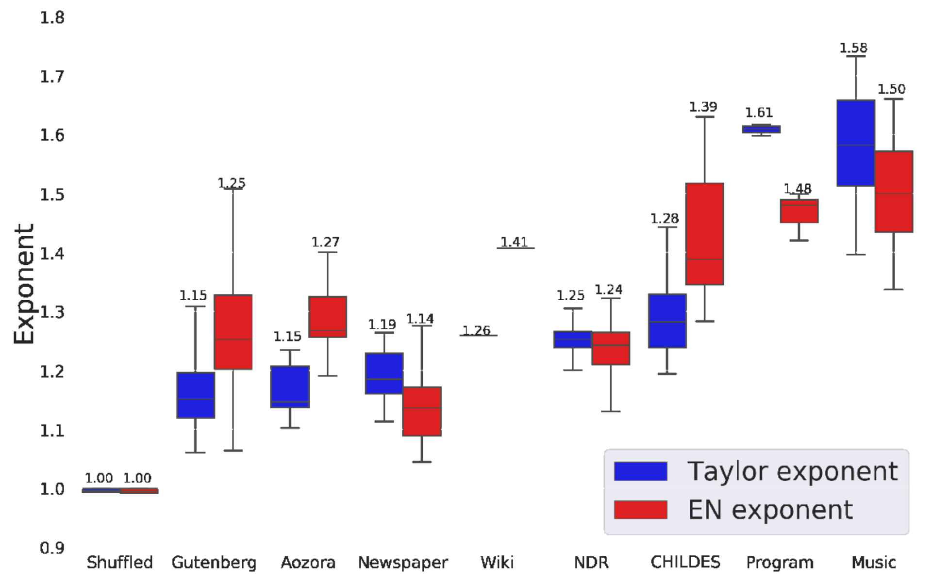
Figure 4 shows the distributions of the exponents with respect to text categories. The horizontal axis indicates the text categories, as listed in the first column of Table 1, while the vertical axis indicates the exponent values. The mean values for every text category are also listed in Table 3 in Appendix D.
Each category has a boxplot for each method. The box edges indicate two quantiles of the data, with the line near the middle of the box indicating the median. The whiskers indicate the maximum and minimum values. The number above each maximum whisker is the median value.
The two leftmost boxes show the results for shuffled data, consisting of 10 different samples acquired from Moby Dick. Following theory, as explained in §2.5, the two boxes are at a value of 1. The figure thus shows how small the variance of the exponents is in that case.
The rest of the figure shows the results for the real data listed in Table 1. Most importantly, not a single sample has a value of 1.
Here, we consider the relation between the text category and the exponents. The second to fourth categories (Gutenberg, Aozora, Newspaper) are results for written text. The Taylor exponents are consistently distributed around 1.15, with the newspaper exponents slightly above those of the literary texts. This is understandable, because among these written forms, similar phrases appear more frequently in newspaper texts, and co-occurrences enlarge the exponent (cf. §2.5). In contrast, the EN exponents vary more widely. Interestingly, the newspaper exponents are lower for the EN method, possibly because of the larger number of rare events. Furthermore, for Project Gutenberg, the variation of the EN exponents is larger than that of the Taylor exponents.
The rest of the figure represents the other categories listed in the third block of Table 1. The fifth category (Wiki) shows results for Wikipedia data, which include the Wikipedia annotations. The Taylor exponents are larger than for the previous categories, which is a result of grammatical annotations in the form of wiki tags. Note that those tags have the tendency to increase co-occurrences (an analysis was given in §2.5). On the other hand, for the EN method, the increase is very large; the exponent is 1.41.
The sixth category in the figure is speech data (the National Diet Record, or NDR, in Japanese). The Taylor exponents are larger than for written text. The EN method shows similar results, but they do not distinguish the written and spoken text, as the exponent values for written text range over a large interval.
The last three categories consist of language spoken by infants, music, and programming language. For all three categories, both exponents are larger than those for the real natural language texts. Taylor’s method gives larger values especially for the programming language data, because of the large co-occurrence effect in program source code.
We performed a statistical test to evaluate whether the differences among text categories were significant. Because the number of texts largely varied among the categories, we conducted a nonparametric statistical test, the Brunner-Munzel method (Brunner and Munzel 2000)11 1 The Kolmogorov-Smirnov test might seem to be a more direct statistical test for examining the similarity of distributions, but it presumes that a distribution has been captured with many sample points. The Brunner-Munzel method is more suitable when the numbers of data points differ largely.. This test examines the difference of the statistical values acquired from two categories. Two samples, and , which are either or values acquired from two sample texts, are each taken from the categories under comparison; then, the null hypothesis is that the probability of and that of are equal.
All categories with at least 10 samples were tested (the Wikipedia and program categories were not tested). Appendix E lists the p-values (Table 4 for Taylor’s method, and Table 5 for the EN method). The results conform to our expectations with a significance level of 0.05. For Taylor’s method, the null hypothesis was validated for the written text (Gutenberg-Aozora, Aozora-Newspaper) and speech (CHILDES-NDR) data 22 2 The null hypothesis was rejected for the Gutenberg-News samples, possibly because these datasets have very large differences in the number of samples.. The null hypothesis was rejected for all other pairs. On the other hand, for the EN method, the null hypothesis was rejected for all pairs except Gutenberg-Aozora. This suggests that the EN method could not capture category differences.
Overall, we can say that Taylor’s method captures categories much better than the EN method does. Such a characteristic captured across categories seems to correspond to some degree of co-occurrence in texts. The correspondence from written to spoken and to other categories suggests a change in complexity. The results presented in this section show how that change is captured by the Taylor exponent but not by the EN exponent. However, the rough results of the EN method are consistent with those of Taylor’s method, giving larger values for the CHILDES, program, and music data than for written texts.
5.2 Effect of Type of Language
Because our data consisted of various language types, we also examined the exponents in relation to language type.


Figure 5 shows scatter plots of the Taylor and EN exponents for all of the natural-language written texts listed in the first and second blocks of Table 1. Each point corresponds to a text, and the Taylor exponent and EN exponent are indicated by the horizontal and vertical coordinates, respectively. The color of each point represents the text’s language. Because the majority of texts are in English, the English texts are in the background, whereas those of the other languages are in the foreground.
The left graph shows the results for words. It indicates the extent to which the EN and Taylor exponents correlate. The Spearman correlation of the two methods is 0.69; thus, the exponents are strongly correlated. The graph also shows how the EN method covers a wider range of exponents compared with Taylor’s method (Figure 4 also showed this).
The graph seems to show a rough clustering of languages, such as the orange points for Chinese and Japanese at the middle right. Therefore, both exponents show some tendency to distinguish languages.
On the other hand, the right graph shows the results for characters. The Spearman correlation between and is 0.44, lower than that for words but still indicating a significant correlation.
The Taylor exponent is around 1 for many of the texts in alphabetic scripts. The analytical results presented in §2.6 indicate that Taylor’s method cannot distinguish texts in alphabetic scripts from an i.i.d. sequence. This is natural, because alphabetic scripts often have fewer than 100 characters, which is too few for a Taylor analysis of the distribution of character types. Once the number of characters reaches the level of Chinese and Japanese, though, the exponents are clearly larger than 1, at around 1.2, which is close to the exponent values of the written texts.
As for the EN method, all the natural language texts have exponents above 1. The EN method thus distinguishes real texts from i.i.d. sequences at the character level. Furthermore, the graph shows that the blue points are clustered at the bottom (around 1.15 on the vertical scale).

Figure 6 shows boxplots of texts for characters with respect to language for the EN exponent . Only results for languages with more than 10 samples are included. From left to right, the languages range from consonantal (Arabic, Hebrew) to alphabetic scripts and ideographs (Chinese and Japanese). The languages are not easy to distinguish; the ranges for English and German include those for Chinese and Japanese.
The statistical test by the Brunner-Munzel method reflects this reality. Here, too, only languages with more than 10 samples were included, and each pair of languages was tested as to whether the exponents were the same. It would be interesting if the test could capture differences among different scripts, but Appendix E shows that the results are not clear. For words, the results for many random language pairs appear to validate the null hypothesis. For characters, the results of the EN method are slightly better: for example, the Japanese-Chinese and Spanish-Italian pairs validate the null hypothesis, but the test results appear almost random.
6 Discussion
6.1 Empirical Pros and Cons of the Two Methods
Thus far, we have discussed the differences in the EN and Taylor methods in terms of qualitative and quantitative evidence. Moreover, Taylor’s method corresponds to the first phase of the EN method, and hence, the methods share a general tendency. Here, we will highlight their differences.
The EN method is statistically more stable. The exponent remains relatively invariant across data sizes. In particular, the method can distinguish a text from an i.i.d. process at any element level. This quality results from summing the variances of all element types. For the same reason, the EN exponent can capture the text category only very roughly.
In contrast, Taylor’s method can distinguish natural language text from an i.i.d. process only at the word level. On the other hand, at the character level, it is not applicable to a target system with a small number of elements, such as an alphabet or a consonantal script, because it considers the distribution of elements. It can, however, distinguish text categories when it is applied to words.
Overall, although Taylor’s method shows some dependency on parameters, if the set of elements is large enough, it is a more direct analysis than the EN method. It also has the possibility of highlighting qualitative differences as categorical distinctions. If the element set consists of fewer than 100 elements, then the EN method can reveal some properties of the system, although the exponent only reflects rough qualitative characteristics of a text.
It is important to learn what characteristics a method highlights. In this study, we revealed subtle differences between the results of Taylor’s method and the EN method when they are used on natural language text, a good target for this purpose as it is interpretable in various ways. We believe that differences such as the ones found here would appear when the methods are applied to targets other than language.
6.2 Interpretation of Exponents as Fractal Dimension
The resulting exponents can be interpreted as a dimension underlying the fluctuation of language. The EN exponent especially has an affinity with the similarity dimension, as a kind of fractal dimension (Mandelbrot 1997; Bunde and Havlin 1996). The similarity dimension is defined for a geometrical object in a metric space. If we suppose that enlarging an object times is equivalent to making copies of the original object, the similarity dimension can be defined as follows:
| (6) |
For example, for a square whose edge length is , doubling would give a square times larger by edge length, but filling this larger square requires of the original squares. Therefore, the similarity dimension is = 2. Similarly, the similarity dimension of a cube is . A famous example is the Koch curve, whose similarity dimension is . For a complex object, this dimension is known not to be an integer.
A text is not a geometrical object, so its length cannot be treated in the same way as a geometrical object defined in a metric space. Nevertheless, it is also true that we often say that a text has a length. The Taylor and EN exponents then suggest a metaphorical interpretation with respect to the fractal dimension. The EN case shows that a text portion that is times longer has times more fluctuation. Accordingly, . Similarly, although the Taylor exponent cannot be interpreted as the similarity dimension, it shows how words occurring times more frequently would fluctuate times more.
The Taylor and EN analyses we have presented here imply that a text does not simply consist of its portions. When the portions are concatenated, they require further editing to unify them into a whole. That is, a text requires linkages across its portions. These linkages generate holistic fluctuations, causing and not to be 1. A text therefore has a property of amplifying fluctuations in a self-similar manner, and Taylor and EN analyses are capable of revealing this property.
7 Conclusion
This article considered the commonalities and differences between Taylor’s method and the Ebeling & Neiman (EN) method in a large-scale study of natural language texts and related data.
Taylor’s method analyzes the distribution of the variance of every element type with respect to the mean within a given segment length. On the other hand, the EN method analyzes how the sum of the variances depends on the segment length. The results of these methods are power laws having respectively Taylor or EN exponents. Either exponent is 1 for an i.i.d. sequence. On the other hand, when a sequence presents some clustering tendency, the exponents become larger: in some cases, such as with consistent co-occurrences and clustered rare words, the exponents reach 2.
Because Taylor’s method can be regarded as the first step of the EN method, the outcomes of the two methods are correlated. Nevertheless, there are differences that derive from the methods’ procedures. Because Taylor’s method is a direct analysis of the distribution of the variances among elements, it can distinguish text categories when it is applied to words. Such a distinction is not so clear with the EN method, possibly because it accumulates the variances of all element types. Both methods show some limited possibility of being able to distinguish languages.
Our findings are based on natural language text as the target of analysis; we chose text because it is interpretable from various aspects. Moreover, we believe that the findings presented in this article apply to other analysis targets besides natural language.
References
- Andelkovic et al. (2001) Andelkovic, Darinka , Seva, Nada , and Moskovljevic, Jasmina (2001). Serbian Corpus of Early Child Language. Laboratory for Experimental Psychology, Faculty of Philosophy, and Department of General Linguistics, Faculty of Philology, University of Belgrade.
- Behrens (2006) Behrens, Heike (2006). The input-output relationship in first language acquisition. Language and Cognitive Processes, 21, 2–24.
- Benedet and Snow (2004) Benedet, Maria and Snow, Catherine (2004). Spanish BecaCESNo Corpus. TalkBank.
- Bol (1995) Bol, Gerard W. (1995). Implicational scaling in child language acquisition : the order of production of Dutch verb constructions, chapter 3, pages 1–13. Amsterdam Series in Child Language Development. Amsterdam: Institute for General Linguistics. editted by Verrips, M. and Wijnen, A.
- Brunner and Munzel (2000) Brunner, Edgar and Munzel, Ullrich (2000). The nonparametric Behrens-Fisher problem: Asymtotic theory and a small-sample approximation. Biometrical Journal, 42, 17–25.
- Bunde and Havlin (1996) Bunde, Armin and Havlin, Shlomo (1996). Fractals and Disordered Systems. Springer.
- Daniels and Bright (1996) Daniels, Peter T. and Bright, William , editors (1996). The World’s Writing Systems. Oxford University Press.
- Ebeling and Neiman (1995) Ebeling, Werner and Neiman, Alexander (1995). Long-range correlations between letters and sentences in texts. Physica A, 215(3), 233–241.
- Eisler et al. (2007) Eisler, Zoltán , Bartos, Imre , and Kertész, Janos (2007). Fluctuation scaling in complex systems: Taylor’s law and beyond. Advances in Physics, 57(1), 89–142.
- Gerlach and Altmann (2014) Gerlach, Martin and Altmann, Eduardo G. (2014). Scaling laws and fluctuations in the statistics of word frequencies. New Journal of Physics, 16(11), 113010.
- Gil and Tadmor (2007) Gil, David and Tadmor, Uri (2007). The MPI-EVA Jakarta Child Language Database. A joint project of the Department of Linguistics, Max Planck Institute for Evolutionary Anthropology and the Center for Language and Culture Studies, Atma Jaya Catholic University.
- Kantelhardt et al. (2002) Kantelhardt, Jan W. , Zschiegner, Stephan A. , Koscielny-Bunde, Eva , Havlin, Shlomo , Bunde, Armin , and Stanley, H. Eugene (2002). Multifractal detrended fluctuation analysis of nonstationary time series. Physica A, 316, 87–114.
- Kobayashi and Tanaka-Ishii (2018) Kobayashi, Tatsuru and Tanaka-Ishii, Kumiko (2018). Taylor’s law for human linguistic sequences. In Proceedings of the 56th Annual Meeting of the Association for Computational Linguistics, pages 1138–1148, Melbourne.
- Lieven et al. (2009) Lieven, Elena , Salomo, Dorothé , and Tomasello, Michael (2009). Two-year-old children’s production of multiword utterances : A usage-based analysis. Cognitive Linguistics, 20(3), 481–508.
- MacWhinney (2000) MacWhinney, Brian (2000). The Childes Project. Psychology Press.
- Mandelbrot (1997) Mandelbrot, Benoit B. (1997). Fractal and Scaling in Finance. Springer.
- Montemurro and Pury (2002) Montemurro, M. and Pury, P.A. (2002). Long-range fractal correlations in literary corpora. Fractals, 10(4), 451–461.
- Oshima-Takane et al. (1995) Oshima-Takane, Yuriko , MacWhinney, Brian , Sirai, Hidetosi , Miyata, Susanne , and Naka, Norio (1995). CHILDES manual for Japanese. Montreal : McGill University.
- Peng et al. (1994) Peng, Chung-Kang , Buldyrev, Sergey V. , Havlin, Shlomo , Simons, Michael , Stanley, H. Eugene , and Goldberger, Ary L. (1994). Mosaic organization of dna nucleotides. Physical Review E, 49, 1685–1689.
- Plunkett and Strömqvist (1992) Plunkett, Kim and Strömqvist, Sven (1992). The acquisition of scandinavian languages. In D. I. Slobin, editor, The Crosslinguistic Study of Language Acquisition, volume 3, pages 457–556. Lawrence Erlbaum Associates.
- Rondal (1985) Rondal, Jean A. (1985). Adult-child interaction and the process of language acquisition. Praeger Publishers.
- Smith (1938) Smith, H. Fairfield (1938). An empirical law describing hetero-geneity in the yields of agricultural crops. Journal of Agriculture Science, 28(1), 1–23.
- Smoczyńska (1986) Smoczyńska, Magdalena (1986). The acquisition of polish. In D. I. Slobin, editor, The Crosslinguistic Study of Language Acquisition, pages 595–686. Lawrence Erlbaum Associates.
- Tanaka-Ishii and Kobahashi (2019) Tanaka-Ishii, Kumiko and Kobahashi, Tatsuru (2019). Addendum: Another explanation about the bounds of the taylor exponent. Journal of Physics Communications, 3(8).
- Tanaka-Ishii and Kobayashi (2018) Tanaka-Ishii, Kumiko and Kobayashi, Tatsuru (2018). Taylor’s law for linguistic sequences and random walk models. Journal of Physics Communications, 2(11).
- Taylor (1961) Taylor, Lionel (1961). Aggregation, variance and the mean. Nature, 189(4766), 732–735.
Appendix A: Procedure to measure mean and variance
Let us segment a sequence into segments of length with no overlap. The appearances of an element are counted in each segment, and the mean and variance are computed from the counts.
is chosen as follows. For Taylor’s method, must be sufficiently smaller than the document length in order to calculate the variance; in other respects, its choice is arbitrary. Among the different values of taken from logarithmic bins, we chose the maximum that could apply to all documents, specifically . For the EN method, the points were taken from segments with an exponentially growing length, e.g., , , where . We set , , .
Appendix B: Datasets
| Texts (Category) | Language | # | Total Length | Mean Vocab Size | ||
| samples | word | char | word | char | ||
| English | 910 | 284945934 | 1421317443 | 17237.7 | 87.4 | |
| French | 66 | 19350770 | 102588196 | 22098.3 | 105.0 | |
| Finnish | 33 | 6518170 | 42270908 | 33597.1 | 86.6 | |
| Chinese | 32 | 20157338 | 43006836 | 15352.9 | 4413.0 | |
| Dutch | 27 | 6935199 | 37021318 | 19159.1 | 97.1 | |
| German | 20 | 4723500 | 26590388 | 24242.3 | 115.2 | |
| Gutenberg (written) | Italian | 14 | 3735326 | 19990753 | 29103.5 | 101.7 |
| Spanish | 12 | 4366047 | 21653921 | 26111.1 | 101.3 | |
| Greek | 10 | 1599692 | 8963014 | 22805.7 | 142.7 | |
| Latin | 2 | 1011487 | 4868576 | 59667.5 | 282.0 | |
| Portuguese | 1 | 261382 | 1333023.0 | 24719.0 | 110.0 | |
| Hungarian | 1 | 198303 | 1037517.0 | 38384.0 | 104.0 | |
| Tagalog | 1 | 208455 | 1193099.0 | 26335.0 | 109.0 | |
| Moby Dick | English | 1 | 254655 | 1255837 | 20473.0 | 78.0 |
| Aozora (written) | Japanese | 13 | 8016804 | 20349717 | 19760.0 | 3050.5 |
| Arabic | 90 | 27008988 | 129553552 | 25200.9 | 93.4 | |
| English | 70 | 21006597 | 115764317 | 21407.3 | 80.1 | |
| Newspaper (written) | Chinese | 30 | 9003127 | 22558321 | 18850.3 | 3494.1 |
| French | 30 | 9002942 | 50625194 | 28134.9 | 99.1 | |
| Hebrew | 10 | 3001046 | 14998734 | 46560.6 | 50.0 | |
| Japanese | 10 | 3001150 | 7737532 | 19833.0 | 2474.0 | |
| Wall Street Journal | English | 1 | 22679513 | 117305668 | 137467.0 | 87.0 |
| Wiki (enwiki8) | tag-annotated | 1 | 14647848 | - | 1430791.0 | - |
| NDR (National | Japanese | 392 | 121781033 | 201204976 | 8882.9 | 1964.0 |
| Diet Record, speech) | ||||||
| CHILDES (speech) | various | 10 | 1934340 | - | 9908.0 | - |
| Programs | various | 4 | 136644076 | - | 838907.8 | - |
| Music | MIDI | 12 | 1631921 | - | 9187.9 | - |
The datasets are publicly available, as listed in Table 1. In general, the data of Taylor or EN analyses should be chosen carefully, because these analyses require a large amount of data, as illustrated in Figure 3. A large-scale text often includes repetitions of large chunks. For such bad data, the analysis would only indicate the poor quality of the data rather than the true nature of the method. From this perspective, the data used in this article were chosen under strict criteria.
The data were categorized into the following three types: single-author literary texts (first block in Table 1), multi-author newspaper corpora (second block), and other kinds of data related to language (third block). The columns of Table 1 indicate the kind of data, the kind of language, the number of samples, the total length (words and characters), and the mean vocabulary size (words and characters). For example, 910 English literary texts were extracted from Project Gutenberg, and the Total Length column lists the total length in words for all 910 texts. Those texts have on average 313,127 words (= 284,945,934 / 910) and 1,42,317,443 characters (= 1,421,317,443 / 910 = 1,561,887), and mean vocabulary sizes of 17,238 words and 87 characters.
The first block of Table 1 lists the names of the literary texts extracted from Project Gutenberg and Aozora Bunko. The row for Moby Dick after Project Gutenberg is the example in the main text (§2.4). The set of literary texts consists of single-author texts extracted from the Project Gutenberg and Aozora Bunko archives and covers 14 languages33 3 Project Gutenberg includes hardly any Japanese literary texts; the Japanese texts were thus acquired from Aozora Bunko.. We initially collected texts above a certain size threshold (1 MB, including annotations). Project Gutenberg splits many of the texts into different volumes; these were manually combined into single texts.
Once the texts were collected, their metadata annotations were eliminated. The PyNLPIR 44 4 https://github.com/jordwest/mecab-docs-en and MeCab 55 5 https://pypi.org/project/PyNLPIR/ applications were used to segment the Chinese and Japanese texts for the word-based analyses. NLTK66 6 https://www.nltk.org was used to tokenize the texts in the other languages.
The word set is often difficult to define: accurate lemmatization is not available for some non-major languages, and it is difficult to capture all the customs of writing systems across languages. We considered that the fairest cross-language approach was to use all tokenized results, without introducing any arbitrary elimination scheme. In other words, conjugated words, capitalized words, misspelled words, and symbols at the word level were all included in the sequences used to produce the results in this article.
| Language | Newspaper |
|---|---|
| English | Wall Street Journal, New York Times, Central News Agency of Taiwan (English), Associated Press (English), Xinhua News Agency (English), Agence-France Presse (English), Los Angeles Times, Washington Post, Washington Post/Bloomberg |
| Arabic | Daily Aaj, Agence France-Presse (Arabic), Al-Ahram, Assabah, Asharq Al-Awsat, Al Hayat, Al-Quds Al-Arabi, Ummah Press, Xinhua News Agency (Arabic) |
| Chinese | People’s Daily, Xinhua News Agency, Central News Agency of Taiwan |
| French | Le Monde, Associated Press (French), Agence France-Presse (French) |
| Hebrew | Haaretz |
| Japanese | Mainichi |
The second block of Table 1 lists data from newspapers, which are characterized as multi-author texts. The above preprocessing scheme was applied to all of the natural language data from these newspapers. Table 2 lists the newspapers used. Many of them are distributed from credible sources such as the Language Data Consortium. In the case of the Wall Street Journal in English, all of the text was used, because it is a standard corpus of highly credible quality. For the other newspapers, 10 non-overlapping portions were extracted in units of articles from random parts of the corpus, so that each portion contained at least 300,000 words. This value of 300,000 words was chosen according to the statistical analysis described in §4, and it met the criteria discussed there.
Daniels and Bright 1996 defined six kinds of writing system used around the globe: alphabetic (Indo-European scripts), abjad (Arabic, Hebrew), abugida (Indian and south Asian scripts), logosyllabary (Chinese), syllabary (Japanese kana), and featural (Korean). This article does not consider the block characters of an abugida or a featural script, because in those cases, one block character is constructed from parts, and the notion of what is “one character” is deemed ambiguous, as a character can be either a component or a combination.
The third block lists the other language-related samples considered in this article, which were introduced for the purpose of comparing the behaviors of the exponents of the two methods.
In the third block, the first row indicates the enwiki8 100-MB dump datasets of Wikipedia, represented by the tag Wiki, consisting of tag-annotated text from English Wikipedia. These data included the annotations made by Wikipedia, for the purpose of observing their effect.
The second row indicates speech data. Obtaining long, clean data is an issue for speech, because speech content changes over time, so sessions are often very short. From the results of a search through various data sources, this article includes data of the National Diet Record (NDR) in Japanese. Records of 250 sessions were used, with each session corresponding to an opening of a National Diet meeting. These data are long and clean; they originally consisted of speech data that were transcribed by professionals.
The third row in the block lists data of the Child Language Data Exchange System (CHILDES). The 10 longest child-directed speech utterances in the CHILDES database were used77 7 The 10 longest utterances were as follows: Thomas (MacWhinney 2000; Lieven et al. 2009), Groningen (Bol 1995), Rondal (Rondal 1985), Leo (Behrens 2006), Ris (Gil and Tadmor 2007), Nanami (Oshima-Takane et al. 1995), Inka (Smoczyńska 1986), Angela (Andelkovic et al. 2001), Beca (Benedet and Snow 2004), and Boteborg (Plunkett and Strömqvist 1992).. The data were preprocessed by extracting only the children’s utterances.
The fourth row lists program source-code data (in the Lisp, Haskell, C++, and Python programming languages) crawled from large representative archives. The data were parsed and stripped of comments written in natural language. The data contain many repetitions, because of the general tendency of programmers to copy and paste sample code. In this sense, the results in this article should be considered only one possible result. It remains an open question how best to reuse programming source code as text data.
Finally, the last row in the third block represents 12 pieces of musical data (long symphonies and so forth) that were transformed from MIDI data into text with the SMF2MML software 88 8 http://shaw.la.coocan.jp/smf2mml/; the annotations were then removed. SMF2MML uses a descriptive method to transcribe the set of sounds occurring at a point in time together with their duration into a word. The transcription approach in this article is only one of the many possible for music.
Appendix C: Dependency of Taylor Exponent on
As reported in Eisler et al. 2007, the Taylor exponent grows as the segment length increases. For texts, it was reported in Kobayashi and Tanaka-Ishii 2018; Tanaka-Ishii and Kobayashi 2018 that depends on the logarithm of . This appendix provides evidence of this from the Wall Street Journal (the data are listed in the first row of the second block in Table 1).

Figure 7 shows the Taylor exponent with respect to . The horizontal axis indicates the logarithm of the segment length, while the vertical axis indicates the Taylor exponent. The figure shows an increasing tendency with respect to , with saturation occurring around . This is due to the fact that a large close to causes the number of segments to decrease. The Taylor exponent is initially when the segment length is . This can be analytically explained as follows (Eisler et al. 2007). Consider the case of . Let be the frequency of a particular word in a segment. We have , because the probability of a specific word appearing in a segment becomes very small. Because , . Then, because or (with =1), . Thus, .
As mentioned in the main text, Taylor’s method can be regarded as the first step of the EN method. Figure 7 shows that the Taylor exponent w.r.t. corresponds to w.r.t .
Appendix D: Mean Taylor and EN Exponents
| Texts | Language | ||||
|---|---|---|---|---|---|
| word | char | word | char | ||
| English | 1.16 | 1.01 | 1.29 | 1.29 | |
| French | 1.14 | 1.04 | 1.23 | 1.24 | |
| Finnish | 1.10 | 1.04 | 1.17 | 1.20 | |
| Chinese | 1.22 | 1.22 | 1.31 | 1.33 | |
| Dutch | 1.14 | 1.04 | 1.22 | 1.24 | |
| German | 1.18 | 1.07 | 1.27 | 1.33 | |
| Gutenberg | Italian | 1.14 | 1.05 | 1.24 | 1.25 |
| Spanish | 1.16 | 1.04 | 1.25 | 1.26 | |
| Greek | 1.16 | 1.02 | 1.18 | 1.22 | |
| Latin | 1.14 | 1.14 | 1.44 | 1.35 | |
| Portuguese | 1.12 | 1.06 | 1.20 | 1.35 | |
| Hungarian | 1.14 | 0.99 | 1.24 | 1.22 | |
| Tagalog | 1.18 | 1.06 | 1.29 | 1.35 | |
| Moby Dick | English | 1.15 | 1.03 | 1.25 | 1.22 |
| Aozora | Japanese | 1.18 | 1.17 | 1.29 | 1.29 |
| Arabic | 1.19 | 1.04 | 1.18 | 1.21 | |
| English | 1.18 | 0.98 | 1.14 | 1.12 | |
| Newspaper | Chinese | 1.22 | 1.22 | 1.17 | 1.19 |
| French | 1.13 | 1.00 | 1.15 | 1.13 | |
| Hebrew | 1.15 | 0.97 | 1.09 | 1.13 | |
| Japanese | 1.24 | 1.18 | 1.26 | 1.30 | |
| National Diet Record | Japanese | 1.25 | 1.22 | 1.21 | 1.23 |
| enwiki8 | tag-annotated | 1.26 | - | 1.41 | - |
| CHILDES | various | 1.36 | - | 1.43 | - |
| Programs | various | 1.58 | - | 1.47 | - |
| Music | MIDI | 1.58 | - | 1.51 | - |
Appendix E: Statistical Test Results for Text Category Pairs
Table 4 and Table 5 list the p-values from the statistical test of the Brunner-Munzel method for every pair of categories with at least 10 samples.
| Shuffled | Gutenberg | Aozora | News | NDR | CHILDES | Music | |
|---|---|---|---|---|---|---|---|
| Shuffled | N/A | 0.000 | 0.000 | 0.000 | 0.000 | 0.000 | 0.000 |
| Gutenberg | - | N/A | 0.347 | 0.000 | 0.000 | 0.000 | 0.000 |
| Aozora | - | - | N/A | 0.205 | 0.000 | 0.000 | 0.000 |
| Newspaper | - | - | - | N/A | 0.000 | 0.000 | 0.000 |
| NDR | - | - | - | - | N/A | 0.116 | 0.000 |
| CHILDES | - | - | - | - | - | N/A | 0.000 |
| Music | - | - | - | - | - | - | N/A |
| Shuffled | Gutenberg | Aozora | News | NDR | CHILDES | Music | |
| Shuffled | N/A | 0.000 | 0.000 | 0.000 | 0.000 | 0.000 | 0.000 |
| Gutenberg | - | N/A | 0.084 | 0.000 | 0.000 | 0.000 | 0.000 |
| Aozora | - | - | N/A | 0.000 | 0.002 | 0.000 | 0.000 |
| Newspaper | - | - | - | N/A | 0.000 | 0.000 | 0.000 |
| NDR | - | - | - | - | N/A | 0.000 | 0.000 |
| CHILDES | - | - | - | - | - | N/A | 0.046 |
| Music | - | - | - | - | - | - | N/A |
Appendix F: Statistical Test Results for Language Pairs
The tables in this section list the p-values from the statistical test of the Brunner-Munzel method for every pair of languages with at least 10 samples. Table 6 and Table 7 are for words, whereas Table 8 is for characters. Because Taylor’s method is not applicable to scripts with a small number of characters, no table is given for that case.
| Arabic | Hebrew | Finnish | Greek | French | Italian | Spanish | English | German | Dutch | Chinese | Japanese | |
| Arabic | N/A | 0.000 | 0.000 | 0.002 | 0.000 | 0.032 | 0.013 | 0.000 | 0.587 | 0.000 | 0.000 | 0.173 |
| Hebrew | - | N/A | 0.000 | 0.542 | 0.057 | 0.111 | 0.285 | 0.018 | 0.041 | 0.008 | 0.000 | 0.051 |
| Finnish | - | - | N/A | 0.004 | 0.404 | 0.000 | 0.000 | 0.000 | 0.000 | 0.000 | 0.000 | |
| Greek | - | - | - | N/A | 0.283 | 0.307 | 0.806 | 0.579 | 0.238 | 0.295 | 0.000 | 0.004 |
| French | - | - | - | - | N/A | 0.259 | 0.864 | 0.000 | 0.013 | 0.498 | 0.000 | 0.000 |
| Italian | - | - | - | - | - | N/A | 0.204 | 0.095 | 0.034 | 0.177 | 0.008 | 0.013 |
| Spanish | - | - | - | - | - | - | N/A | 0.316 | 0.099 | 0.702 | 0.000 | 0.003 |
| English | - | - | - | - | - | - | - | N/A | 0.226 | 0.021 | 0.000 | 0.002 |
| German | - | - | - | - | - | - | - | - | N/A | 0.025 | 0.079 | 0.477 |
| Dutch | - | - | - | - | - | - | - | - | - | N/A | 0.000 | 0.000 |
| Chinese | - | - | - | - | - | - | - | - | - | - | N/A | 0.350 |
| Japanese | - | - | - | - | - | - | - | - | - | - | - | N/A |
| Arabic | Hebrew | Finish | Greek | French | Italian | Spanish | English | German | Dutch | Chinese | Japanese | |
| Arabic | N/A | 0.000 | 0.321 | 0.634 | 0.296 | 0.013 | 0.000 | 0.000 | 0.027 | 0.001 | 0.000 | 0.000 |
| Hebrew | - | N/A | 0.000 | 0.001 | 0.000 | 0.000 | 0.000 | 0.000 | 0.000 | 0.000 | 0.000 | 0.000 |
| Finnish | - | - | N/A | 0.423 | 0.092 | 0.006 | 0.000 | 0.000 | 0.008 | 0.001 | 0.000 | 0.000 |
| Greek | - | - | - | N/A | 0.723 | 0.046 | 0.012 | 0.001 | 0.035 | 0.141 | 0.032 | 0.000 |
| French | - | - | - | - | N/A | 0.056 | 0.000 | 0.000 | 0.064 | 0.022 | 0.004 | 0.000 |
| Italian | - | - | - | - | - | N/A | 0.691 | 0.320 | 0.554 | 0.427 | 0.826 | 0.193 |
| Spanish | - | - | - | - | - | - | N/A | 0.392 | 0.827 | 0.112 | 0.677 | 0.146 |
| English | - | - | - | - | - | - | - | N/A | 0.902 | 0.002 | 0.031 | 0.155 |
| German | - | - | - | - | - | - | - | - | N/A | 0.267 | 0.421 | 0.984 |
| Dutch | - | - | - | - | - | - | - | - | - | N/A | 0.354 | 0.000 |
| Chinese | - | - | - | - | - | - | - | - | - | - | N/A | 0.037 |
| Japanese | - | - | - | - | - | - | - | - | - | - | - | N/A |
| Arabic | Hebrew | Finnish | Greek | French | Italian | Spanish | English | German | Dutch | Chinese | Japanese | |
| Arabic | N/A | 0.000 | 0.558 | 0.118 | 0.268 | 0.110 | 0.002 | 0.000 | 0.000 | 0.000 | 0.000 | 0.000 |
| Hebrew | - | N/A | 0.000 | 0.000 | 0.000 | 0.000 | 0.000 | 0.000 | 0.000 | 0.000 | 0.000 | 0.000 |
| Finnish | - | - | N/A | 0.165 | 0.759 | 0.339 | 0.007 | 0.000 | 0.000 | 0.015 | 0.002 | 0.000 |
| Greek | - | - | - | N/A | 0.323 | 0.955 | 0.169 | 0.087 | 0.023 | 0.594 | 0.177 | 0.046 |
| French | - | - | - | - | N/A | 0.232 | 0.014 | 0.000 | 0.000 | 0.030 | 0.000 | 0.000 |
| Italian | - | - | - | - | - | N/A | 0.497 | 0.312 | 0.086 | 0.699 | 0.792 | 0.291 |
| Spanish | - | - | - | - | - | - | N/A | 0.857 | 0.130 | 0.334 | 0.736 | 0.901 |
| English | - | - | - | - | - | - | - | N/A | 0.142 | 0.117 | 0.490 | 0.588 |
| German | - | - | - | - | - | - | - | - | N/A | 0.038 | 0.077 | 0.175 |
| Dutch | - | - | - | - | - | - | - | - | - | N/A | 0.374 | 0.062 |
| Chinese | - | - | - | - | - | - | - | - | - | - | N/A | 0.923 |
| Japanese | - | - | - | - | - | - | - | - | - | - | - | N/A |