Self-organized Criticality in Multi-pulse Gamma-Ray Bursts
Front. Phys. ???, ?? (2020)
DOI ???
Research article
1. Purple Mountain Observatory, Chinese Academy of Sciences, Nanjing 210023, China
2. University of Chinese Academy of Sciences, Beijing 100049, China
3. Theoretical Division, Los Alamos National Laboratory, Los Alamos, NM 87545, USA
4. College of Physics and Electronic Engineering, Nanyang Normal University, Nanyang, Henan 473061, China
5. School of Astronomy and Space Science, University of Science and Technology of China, Hefei, Anhui 230026, China
6. School of Astronomy and Space Science, Nanjing University, Nanjing 210023, China
7. Institute of Astronomy and Astrophysics, University of Tübingen, Auf der Morgenstelle 10, D-72076,Tübingen
Corresponding author E-mail: ∗leeyp2009@gmail.com, ∗∗gengjinjun@nju.edu.cn, xfwu@pmo.ac.cn
The variability in multi-pulse gamma-ray bursts (GRBs) may help to reveal the mechanism of underlying processes from the central engine. To investigate whether the self-organized criticality (SOC) phenomena exist in the prompt phase of GRBs, we statistically study the properties of GRBs with more than 3 pulses in each burst by fitting the distributions of several observed physical variables with a Markov Chain Monte Carlo approach, including the isotropic energy , the duration time and the peak count rate of each pulse. Our sample consists of 454 pulses in 93 GRBs observed by the CGRO/BATSE satellite. The best-fitting values and uncertainties for these power-law indices of the differential frequency distributions are: , and , while the power-law indices in the cumulative frequency distributions are: , and . We find that these distributions are roughly consistent with the physical framework of a Fractal-Diffusive, Self-Organized Criticality (FD-SOC) system with the spatial dimension and the classical diffusion =1. Our results support that the jet responsible for the GRBs should be magnetically dominated and magnetic instabilities (e.g., kink model, or tearing-model instability) lead the GRB emission region into the SOC state.
Keywords gamma-ray burst: general -methods: statistical
PACS numbers 98.70.Rz, 02.70.Rr
1 Introduction
Gamma-ray bursts (GRBs) are extremely energetic events occurring at the cosmological distance. The observed GRB lightcurves usually consist of several pulses characterized by highly temporal variabilities. It is well accepted that the prompt gamma-ray emission is generated by internal dissipation processes while the later afterglow is produced through the shock wave interacting with the surrounding medium. There is a consensus that long GRBs originate from the collapse of massive stars [1], while short GRBs are from mergers of two compact objects such as binary neutron stars or black hole-neutron star binaries [2, 5, 3, 4, e.g.]. The nature of GRB’s central engine has remained mysterious. The central engine is popularly supposed to be a black hole surrounded by a hyper-accreting disk [6] or a millisecond magnetar [5], but remains uncertain from case to case. On the other hand, the presence of X-ray flares after the prompt gamma-ray emission indicates the GRB central engine may not cease all activities after the main burst phase [7, 5, 8, 9, 10, e.g.].
The self-organized criticality (SOC) phenomena are ubiquitous, and they are commonly observed in many astrophysical processes, such as solar flares [11], magnetospheric substorms, lunar craters, pulsar glitches, and fast radio bursts [12, 13, 14], etc (see [15, 16] for a review). The general definition of SOC is a critical state of a nonlinear energy dissipation system that is slowly and continuously driven towards a critical value of a system-wide instability threshold, producing scale-free, fractal-diffusive, and intermittent avalanches [15, 17, 18]. The SOC phenomena could be identified and diagnosed by analyzing the power-law or power-law like frequency distributions of relevant scale-free parameters [19, 20, 15, 16].
Some SOC phenomena in GRBs have been discussed in the literature. The frequency distributions of energy/waiting time11 1 The general definition of waiting time is the time interval between two subsequent bursts. for GRB X-ray flares exhibit power-law tails very similar to those of solar X-ray flares [21] indicating that the central engine activity of GRBs might be a magnetic reconnection-driven SOC system like that happens on the Sun. It was later revealed that statistical properties of energy, duration, peak flux, and waiting time for X-ray flares from different sources (the Sun, GRBs, Swift J1644+57, Sgr A∗, and M87) could be wholly explained by the SOC model [22]. Also, the statistical similarities between those sources imply that all of the X-ray flares are consistent with magnetic reconnection events. The dimensionality of the SOC process in Sgr A∗ X-ray flares is discussed [23]. The waiting time distributions of both -ray pulses and X-ray flares of GRBs were systematically analyzed and argued that it is not proper to use the SOC mechanism as the interpretation to GRBs [24]. However, Yi et al. [25] comprehensively studied GRB X-ray flares observed by the Swift satellite, and their results supported the SOC phenomena in GRBs. Moreover, it is found that these statistical properties are similar to those of the X-ray flares, which indicates that GRB optical flares and X-ray flares may share a common physical origin [26]. Besides, the power density spectra (PDSs) of GRB prompt lightcurves (with a power-law index value of ) indicate the bursts themselves have a self-similar temporal structure [27].
Some studies suggest that X-ray flares and the gamma-ray prompt emission may share a common origin, i.e., relativistic jets [28, 29]. It is straightforward to ask whether the SOC phenomena exist in the GRB prompt emission and if so, whether the SOC behavior of multiple-pulses in the prompt emission is consistent with that of X-ray flares, and what causes this SOC behavior. This motivates us further to investigate the statistical properties of multiple pulses to explore the SOC behavior in the main prompt emission of GRBs.
The most interesting statistical characteristics of the SOC phenomena are scale-free power-law or the power-law-like size distributions (or frequency distributions) of the physical parameters of the system ([30] and the references therein).
In this study, we investigate the statistical characteristics of GRBs with multiple pulses in their prompt -ray lightcurves. The structure of this article is as follows. We present the selection criterion for our GRB sample in Section 2. In Section 3, we study the frequency distributions of several physical quantities, including the energy, the duration time, and the peak count rates of the pulses of GRBs. Finally, in Section 4, we discuss the implication of the statistical results and summarize our conclusions. Throughout this work, we assume a flat CDM universe with the cosmological parameters , , and .
2 Sample and data reduction
GRB lightcurves are highly complex and diverse, varying from a smooth single pulse to spiky multi-pulses. The pulses in the prompt emission should be the imprints of activities of the GRB central engine. Here, we investigate the statistical distributions of three physical variables of GRB pulses, including the isotropic energy , the duration time , and the peak count rate .
As the Burst and Transient Source Explorer (BATSE; [31, 32]) onboard in the Compton Gamma-Ray Observatory (CGRO; [33]) has a wider energy range and a lower photon detection threshold, we collect the GRB sample from BATSE, rather than other instruments like HETE-2, Swift, or Fermi. From the BATSE GRB catalog [34], we select the bursts whose lightcurves have at least three pulses. For these bursts, their pseudo redshifts are obtained from the catalog [35], which are estimated based on the -luminosity relation. Since spectral parameters are essential to derive the -correction to the and , we choose the bursts that have spectral parameters in the BATSE 5B GRB spectral catalog [36]. With this selection criterion, we finally collect 454 pulses in a sample of 93 GRBs.
-correction to burst energy in its cosmological rest frame should be considered in our calculations. For a burst at redshift of , the corrected isotropic energy is written as
| (1) |
where is the pulse fluence, and is the luminosity distance, and the spectral function is the empirical Band function [37]. The spectral parameters for could be referred from the catalog [34]. Note that the pseudo redshifts of our sample were estimated based on the empirical luminosity relation, in which the integration of -corrections factor is performed from 30 keV and keV [35]. To keep the consistence, we here adopt the same range of integration [38, 35]. and are 25 keV and 300 keV, respectively, because the pulse fluence is observed in this energy range.
For the pulse duration in the source rest frame, it is , where is the observed pulse width obtained from Table 1 in the catalog [34]. Note that here is based on time intervals between times when the pulse intensity is , rather than , and is the pulse amplitude [39]. The pulse peak count rate (in unit of ) in the rest frame is calculated as
| (2) |
where is the peak flux in 64 ms bin.
3 SOC analyses
While an ideal power-law distribution function is commonly used in the standard SOC models, most observed frequency distributions of empirical data are not consistent with an ideal power law. Hence, we will use the thresholded power-law distribution function [30] to analyze the data in our work.
In general, for the number of events N, the observed differential distribution could be well described with a so-called thresholded power-law distribution
| (3) |
where is a constant by considering the threshold effects (e.g., incomplete sampling below , background contamination), and are the minimum and maximum values of , respectively. The uncertainty of the differential distribution is given by
| (4) |
where is the event number in the -th bin, and is the bin size. And for , the corresponding cumulative distribution function (CDF) is written as
| (5) |
where is the total number of events. The uncertainty of the cumulative distribution in a given bin is estimated with
| (6) |
where is the number of events of the bin.
For a fractal-diffusive system, the statistical properties of the event duration (), event intensity () and event energy() are critical for determining the SOC structures [15]. In the following, we discuss the physical implication of the prompt pulse variables’ differential distributions in the framework of FD-SOC model. For the fractal dimension of avalanches, the FD-SOC theory predicts the indices of differential distributions for , and [15] as
| (7) |
where is the Euclidean space dimensionality, is the diffusion parameter, is the mean value of a fractal dimension, which is calculated by [20].
We explore the differential size distributions and the cumulative size distributions of observed physical variables (i.e., , , and ), and fit them with the theoretical model. We apply a uniformly logarithmic binning for the differential and the cumulative distributions. The method for determining the numbers of bins is similar to that in Li et al. [23]. For the differential distributions, the bins that have no events are omitted.
We obtain the best fitting parameter by minimizing the reduced for the differential distribution function,
| (8) |
The for the cumulative distribution function
| (9) |
where is the number of logarithmic bins, and is the number of the free parameters. and are the corresponding observed values for the differential distribution and the cumulative distribution, respectively.
In equations 3-5, there are two crucial parameters, i.e., and . It has been revealed [30] that the cumulative distributions turn out to be highly degenerate over . Therefore, when taking as a free parameter together with to fit the cumulative distributions, could not be well constrained. Here we take the same as in the differential distribution with the same binning. The position of emerging breakpoint shown in the differential distribution is taken as the value of , as shown in the left panels of Figs. 1 - 3. This is primarily based on the definition of , which was introduced to account for the deviation from an ideal power-law like behavior at the lower part of the differential distribution. The fitting parameters of these two kinds of differential distributions can be determined via the emcee algorithm ( Python implementation of Markov chain Monte Carlo fitting technique, [40]) if is fixed.
The differential distribution of the pulse is displayed in the left panel of Figure 1 with erg, and the power-law index fitted using Equation (3) yields (=2.7122 2 Note that the MCMC fitting and the calculation of are performed by considering the data above only). The right panel of Figure 1 illustrates the corresponding cumulative distribution. With the threshold determined by the differential distribution, the best-fitting power-law index of the cumulative distribution is (=1.55).
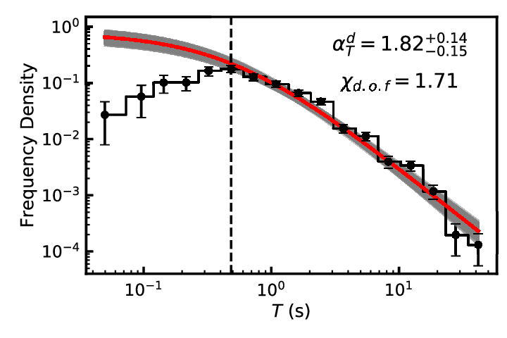
The differential distribution of the pulse duration time () for the -ray multi-pulses sample is displayed in the left panel of Figure 2, which gives the best-fitting index as (=1.71) given the threshold value to be 0.48 s. The corresponding cumulative distribution is shown in the right panel of Figure 2, gives the best-fitting index as (=1.05).
Also, in Figure 3, it is shown that the differential distribution and the cumulative distribution of could be fitted with indices of (=1.14), and (=0.59) respectively, given the threshold value to be counts .
All the results above have quoted a 3 uncertainty for the best fitted power-law index. The derived indices from the fits to both the differential and cumulative distributions are generally consistent within the error bars. It is obvious from Figures 1 3 that the values of for the differential size distributions are larger than those in the cumulative size distributions. The major reason is that the cumulative size distributions would contain favorably more events in each bin than the differential distributions.
The choice of from the data itself would lead to the relatively large =2.71 in the left panel of Figure 1 since is deeply affected by the effect of incomplete sampling and background contamination.
In the framework of the FD-SOC model, we obtain , and 1.7 according to Equation (7) by taking the three-dimensional space () and the classical diffusion (). Comparing to our results, it is found that the derived and are well consistent with the prediction of the FD-SOC model and also roughly consistent with the model prediction. is derived from 64 ms peak flux (see equation 2). However, is replaced by an averaged flux over the pulse duration for several long-timescale pulses in the catalog. Considering that the averaged flux over the pulse duration is relatively fainter than the flux determined in short time interval [41], is expected to be steeper than its predicted value.




4 Discussions and conclusion
In this paper, we have compiled 454 prompt -ray pulses in 93 GRBs observed by the CGRO-BATSE satellite within ten years. The reason why we select the mutiple-pulses dected by the CGRO-BATSE satellite as the only sample source because of its lower photon detection threshold (observed pulses are more distinct) compared with other detectors. At the same time, the total number of GRBs in our sample is limited by the number that have pseudo redshifts which were served as a distance indicator.
By analyzing the temporal properties (i.e., , and ) of these pulses, we presented that the differential and the cumulative thresholded differential distributions of GRB temporal properties could be well understood within the physical framework of a fractal-diffusive, self-organized criticality (FD-SOC) model, which is generally consistent with the previous works on the SOC behavior in GRB X-ray flares [21, 22, 25, 26]. However, the statistical results favor a spatial dimension of of the SOC system for prompt properties, rather than a spatial dimension of for the case of X-ray flares [21].
The positive thresholds of these physical parameters in three distributions (see Figures 1 3) suggest that the statistical results of SOC behavior among multiple pulses in the prompt emission are slightly contaminated by the event-unrelated background [30].
Pulses are building blocks of one GRB event. Due to the highly overlapping effect, it is difficult to identify the pulses from complex lightcurves. In this analysis, we adopt a sample from [34] and present SOC analysis. Note that scale-free is a very important characteristic of a SOC system. Although extracting pulses from lightcurves highly depends on the empirical pulse model and the instrument threshold, our analysis based on the uniform criteria could give insights to evaluating the SOC nature of GRBs.
Another effect is that the physical threshold of the instability of pulses in the prompt emission of GRBs. In a SOC system, owing to some driving force, the subsystems will self-organize to a critical state at which a small perturbation can trigger an avalanche-like chain reaction of any size (namely the instability). For the GRB prompt emission pulses studied in this work, the instability of the SOC behavior is closely related to the jet composition (thermally or magnetically dominant) and the central engine models (hyper-accreting black hole or rapidly spinning magnetar). If the jet is thermally dominated [42, 43, 44, 45, 46] and produced by the neutrino annihilation from the accretion disk around the black hole, the instability is likely to be the thermal instability of the accretion disk. If the jet is dominated by magnetic fields [47, 48, 49] and launched from a magnetar or a black hole (i.e., through the Blandford-Znajek mechanism [50]), the SOC behavior may be determined by the magnetic reconnection instabilities, such as the kink-mode or tearing-mode instability.
It is interesting to notice that both the GRB prompt emission and X-ray flare resemble a SOC system, but favor a different spatial dimension parameter respectively. This apparent contradiction could be also naturally explained within the scenario of a magnetic-dominated jet. Some studies have suggested that X-ray flares and the gamma-ray prompt emission may share a common origin, i.e., X-ray flares also come from relativistic jets. In such a scenario, the magnetic reconnection is supposed to drive the current sheets, from which the electrons are accelerated to emit observed photons. However, the prompt burst phase and flare episodes should belong to different active stages of the central engine (e.g., [51]). During the early prompt phase, the turbulent magnetic reconnection will produce mini-emitters [52, 53] by the magnetic instabilities (tearing/plasmoids). The runaway growth of these mini-emitters is in a 3-dimensional (or isotropic) form due to the existence of turbulence, resulting in a SOC system with a dimension of . For late X-ray flares, the magnetic field reconnection topology for the dissipation region should be 1-dimensional (i.e., ) [21]. The emission site of gamma-ray emission differs from that of X-ray flares, which makes the dimension of their magnetic reconnection different, i.e., the bursts in the prompt emission might correspond to 3-dimensional magnetic reconnection, while the X-ray flares might be 1-dimensional magnetic reconnection. Therefore, our statistical results provide an indirect clue to identify the jet composition and the radiation mechanism of GRBs.
In this work, the GRBs are selected from the same instrument, and the backgrounds are well deducted when deriving the lightcurve of every burst, which makes the observational bias of our sample to be minimal. On the other hand, it seems to be a critical issue when we are gathering the pulses from different GRBs to perform analyses while these GRBs may have different physical progenitors. In principle, it is better to analyze the pulses within a single burst. However, we found that there are no enough pulses to perform the statistics within a single burst. Fortunately, the selection criterion of our sample, i.e., having 3 pulses in each burst, excludes any short GRB from our sample. All the bursts in our sample are long GRBs indeed, and they are theoretically believed to come from the collapse of the massive stars. Thus the bias of our results due to the internal difference between each burst is not so significant given the same origin.
To summarize, we draw a tentative conclusion that our statistical results are explained in the theoretical prediction of a self-organized criticality system with the classical diffusion, the spatial dimension , which are generally consistent with statistical results of various black hole systems including GRBs, TDE Swift J1644+57, Sgr A∗, M87. They can be explained by a three-dimensional SOC model [22], despite the dimension of our result is different from that of previous work [21, 22, 25, 26], which implies that the relativistic jets may be magnetically dominated, consistent with our previous work [48].
Although only the BATSE sample of GRBs with pseudo redshifts are adopted for SOC analyses, we anticipate that the Swift sample of GRBs with detected redshifts and corresponding analysis may be also interesting. In the future, it is worthy to explore the SOC behavior in the prompt emission and X-ray flares simultaneously observed with a large sample of GRBs detected by Swift satellite, which may help to probe into the activities of the central engine from the prompt phase to afterglow phase.
Acknowledgements This work is partially supported by the National Natural Science Foundation of China (grant Nos. 11673068, 11725314, U1831122, 11703064, 11903019, and U1938116), the Shanghai Sailing Program (No. 17YF1422600), the Youth Innovation Promotion Association (2017366), the Key Research Program of Frontier Sciences (grant Nos. QYZDB-SSW-SYS005 and ZDBS-LY-7014), and the Strategic Priority Research Program “Multi-waveband gravitational wave Universe” (grant No. XDB23000000) of the Chinese Academy of Sciences.
References
- Meszaros and Rees [1992] P. Meszaros, and M. J. Rees Tidal Heating and Mass Loss in Neutron Star Binaries: Implications for Gamma-Ray Burst Models, ApJ. 397,570 (1992)
- Paczynski [1986] B. Paczynski, Gamma-ray bursters at cosmological distances, ApJL. 308,L43 (1986)
- Metzger et al. [2011] B. D. Metzger, D. Giannios, and S. Horiuchi Heavy nuclei synthesized in gamma-ray burst outflows as the source of ultrahigh energy cosmic rays, MNRAS. 415,2495 (2011)
- Goldstein et al. [2017] A. Goldstein, P. Veres, E. Burns, et al., An Ordinary Short Gamma-Ray Burst with Extraordinary Implications: Fermi-GBM Detection of GRB 170817A, ApJL. 848,L14 (2017)
- Dai et al. [2006] Z. G. Dai, X. Y. Wang, X. F. Wu, and B. Zhang X-ray Flares from Postmerger Millisecond Pulsars, Sci. 311,1127 (2006)
- MacFadyen and Woosley [1999] A. I. MacFadyen and S. E. Woosley Collapsars: Gamma-Ray Bursts and Explosions in “Failed Supernovae”, ApJ. 524,262 (1999)
- Burrows et al. [2005] D. N. Burrows, P. Romano, A. Falcone, et al., Bright X-ray Flares in Gamma-Ray Burst Afterglows, Sci. 309,1833 (2005)
- Liang et al. [2006] E. W. Liang, B. Zhang, P. T. O’Brien, et al., Testing the Curvature Effect and Internal Origin of Gamma-Ray Burst Prompt Emissions and X-Ray Flares with Swift Data, ApJ. 646,351 (2006)
- Zhang et al. [2006] B. Zhang, Y. Z. Fan, J. Dyks, et al., Physical Processes Shaping Gamma-Ray Burst X-Ray Afterglow Light Curves: Theoretical Implications from the Swift X-Ray Telescope Observations, ApJ. 642,354 (2006)
- Liu and Mao [2019] C.Liu, and J. Mao GRB X-Ray Flare Properties among Different GRB Subclasses, ApJ. 884,59 (2019)
- Goodman et al. [2020] M. L. Goodman, C. Kwan, B. Ayhan, and E. L. Shang A new approach to solar flare prediction, FrPhy. 15,34601 (2020)
- Wang and Yu [2017] F. Y. Wang, and H. Yu SGR-like behaviour of the repeating FRB 121102, JCAP. 2017,023 (2017)
- Li et al. [2019] B. Li, L.-B. Li, Z.-B. Zhang, et al., Statistical properties of the repeating fast radio burst source FRB 121102, arXiv.arXiv:1901.03484 (2019)
- Zhang et al. [2019] G. Q. Zhang, F. Y. Wang, and Z. G. Dai Similar behaviors between FRB 121102 and solar type III radio bursts, arXiv.arXiv:1903.11895 (2019)
- Aschwanden [2014] M. J. Aschwanden, A Macroscopic Description of a Generalized Self-organized Criticality System: Astrophysical Applications, ApJ. 782,54 (2014)
- Aschwanden et al. [2016] M. J. Aschwanden, N. B. Crosby, M. Dimitropoulou, et al., 25 Years of Self-Organized Criticality: Solar and Astrophysics, SSRv. 198,47 (2016)
- Bak et al. [1987] P. Bak, C. Tang, and K. Wiesenfeld Self-organized criticality: An explanation of the 1/f noise, PhRvL. 59,381 (1987)
- Bak et al. [1988] P. Bak, C. Tang, and K. Wiesenfeld Self-organized criticality, PhRvA. 38,364 (1988)
- Aschwanden and McTiernan [2010] M. J. Aschwanden, and J. M. McTiernan Reconciliation of Waiting Time Statistics of Solar Flares Observed in Hard X-rays, ApJ. 717,683 (2010)
- Aschwanden [2012] M. J. Aschwanden, A statistical fractal-diffusive avalanche model of a slowly-driven self-organized criticality system, A&A. 539,A2 (2012)
- Wang and Dai [2013] F. Y. Wang, and Z. G. Dai Self-organized criticality in X-ray flares of gamma-ray-burst afterglows, NatPh. 9,465 (2013)
- Wang et al. [2015] F. Y. Wang, Z. G. Dai, S. X. Yi, and S. Q. Xi Universal Behavior of X-Ray Flares from Black Hole Systems, ApJS. 216,8 (2015)
- Li et al. [2015] Y.-P. Li, F. Yuan, Q. Yuan, et al., Statistics of X-Ray Flares of Sagittarius A*: Evidence for Solar-like Self-organized Criticality Phenomena, ApJ. 810,19 (2015)
- Guidorzi et al. [2015] C. Guidorzi, S. Dichiara, F. Frontera, et al., A Common Stochastic Process Rules Gamma-ray Burst Prompt Emission and X-ray Flares, ApJ. 801,57 (2015)
- Yi et al. [2016] S.-X. Yi, S.-Q. Xi, H. Yu, et al., Comprehensive Study of the X-Ray Flares from Gamma-ray Bursts Observed by Swift, ApJS. 224,20 (2016)
- Yi et al. [2017] S.-X. Yi, H. Yu, F. Y. Wang, and Z.-G. Dai Statistical Distributions of Optical Flares from Gamma-Ray Bursts, ApJ. 844,79 (2017)
- Beloborodov et al. [2000] A. M. Beloborodov, B. E. Stern, and R. Svensson Power Density Spectra of Gamma-Ray Bursts, ApJ. 535,158 (2000)
- Uhm and Zhang [2015] Z. L. Uhm, and B. Zhang On the Curvature Effect of a Relativistic Spherical Shell, ApJ. 808,33 (2015)
- Geng et al. [2018] J.-J. Geng, Y.-F. Huang, X.-F. Wu, L.-M. Song, and H.-S. Zong Probing Magnetic Fields of GRB X-Ray Flares with Polarization Observations, ApJ. 862,115 (2018)
- Aschwanden [2015] M. J. Aschwanden, Thresholded Power law Size Distributions of Instabilities in Astrophysics, ApJ. 814,19 (2015)
- Fishman et al. [1989] G. J. Fishman, C. A. Meegan, R. B. Wilson, et al., The BATSE Experiment for the GRO - Solar Flare Hard X-Ray and Gamma-Ray Capabilities, BAAS. 21,860 (1989)
- Meegan et al. [1992] C. A. Meegan, G. J. Fishman, R. B. Wilson, et al., Spatial distribution of -ray bursts observed by BATSE, Natur. 355,143 (1992)
- Gehrels et al. [1994] N. Gehrels, E. Chipman, and D. Kniffen The Compton Gamma Ray Observatory, ApJS. 92,351 (1994)
- Hakkila and Preece [2011] J. Hakkila, and R. D. Preece Unification of Pulses in Long and Short Gamma-Ray Bursts: Evidence from Pulse Properties and Their Correlations, ApJ. 740,104 (2011)
- Yonetoku et al. [2004] D. Yonetoku, T. Murakami, T. Nakamura, and 3 colleagues Gamma-Ray Burst Formation Rate Inferred from the Spectral Peak Energy-Peak Luminosity Relation, ApJ. 609,935 (2004)
- Goldstein et al. [2013] A. Goldstein, R. D. Preece, R. S. Mallozzi, et al., The BATSE 5B Gamma-Ray Burst Spectral Catalog, ApJS. 208,21 (2013)
- Band et al. [1993] D. Band, J. Matteson, L. Ford, et al., BATSE Observations of Gamma-Ray Burst Spectra. I. Spectral Diversity, ApJ. 413,281 (1993)
- Amati et al. [2002] L. Amati, F. Frontera, M. Tavani, et al., Intrinsic spectra and energetics of BeppoSAX Gamma-Ray Bursts with known redshifts, A&A. 390,81 (2002)
- Norris et al. [2005] J. P. Norris, J. T. Bonnell, D. Kazanas, et al., Long-Lag, Wide-Pulse Gamma-Ray Bursts, ApJ. 627,324 (2005)
- Foreman-Mackey et al. [2013] D. Foreman-Mackey, D. W. Hogg, D. Lang, and J. Goodman emcee: The MCMC Hammer, PASP. 125,306 (2013)
- Lyu et al. [2015] F. Lyu, Y. Wang, Y. Liang, et al., Comparison between the time-integrated spectrum and the peak time spectrum of gamma-ray bursts and possible implications, SCPMA. 58,5575 (2015)
- Meszaros and Rees [1993] P. Meszaros and M. J. Rees Relativistic Fireballs and Their Impact on External Matter: Models for Cosmological Gamma-Ray Bursts, ApJ. 405,278 (1993)
- Piran et al. [1993] T. Piran, A. Shemi, and R. Narayan Hydrodynamics of Relativistic Fireballs, MNRAS. 263,861 (1993)
- Hou et al. [2018] S.-J. Hou, B.-B. Zhang, Y.-Z. Meng, et al., Multicolor Blackbody Emission in GRB 081221, ApJ. 866,13 (2018)
- Meng et al. [2018] Y.-Z. Meng, J.-J. Geng, B.-B. Zhang, et al., The Origin of the Prompt Emission for Short GRB 170817A: Photosphere Emission or Synchrotron Emission?, ApJ. 860,72 (2018)
- Meng et al. [2019] Y.-Z. Meng, L.-D. Liu, J.-J. Wei, X.-F. Wu, and B.-B. Zhang The Time-resolved Spectra of Photospheric Emission from a Structured Jet for Gamma-Ray Bursts, ApJ. 882,26 (2019)
- Zhang and Yan [2011] B. Zhang, and H. Yan The Internal-collision-induced Magnetic Reconnection and Turbulence (ICMART) Model of Gamma-ray Bursts, ApJ. 726,90 (2011)
- Lyu et al. [2014] F. Lyu, E.-W. Liang, Y.-F. Liang, et al., Distributions of Gamma-Ray Bursts and Blazars in the L p-E p-Plane and Possible Implications for their Radiation Physics, ApJ. 793,36 (2014)
- Uhm and Zhang [2014] Z. L. Uhm, and B. Zhang Fast-cooling synchrotron radiation in a decaying magnetic field and -ray burst emission mechanism, NatPh. 10,351 (2014)
- Blandford and Znajek [1977] R. D. Blandford, and R. L. Znajek Electromagnetic extraction of energy from Kerr black holes., MNRAS. 179,433 (1977)
- Hu et al. [2014] Y.-D. Hu, E.-W. Liang, S.-Q. Xi, and 4 colleagues Internal Energy Dissipation of Gamma-Ray Bursts Observed with Swift: Precursors, Prompt Gamma-Rays, Extended Emission, and Late X-Ray Flares, ApJ. 789,145 (2014)
- Zhang and Zhang [2014] B. Zhang and B. Zhang Gamma-Ray Burst Prompt Emission Light Curves and Power Density Spectra in the ICMART Model, ApJ. 782,92 (2014)
- Lazarian et al. [2020] A. Lazarian,, G. L. Eyink, A. Jafari, et al., 3D turbulent reconnection: Theory, tests, and astrophysical implications, PhPl. 27,012305 (2020)