I Introduction
After the striking neutron star merging GW170817 event
GBM:2017lvd, which was followed by a kilonova, the fact
that the gravitational waves arrived almost simultaneously with
the electromagnetic radiation emitted by the kilonova, it was
obvious that the gravitational wave speed was nearly equal
to that of light’s, that is in natural units. This fact
has put several generalizations of Einstein’s theory of relativity
into peril, since several extended theories of gravity predict a
gravitational wave speed different from that of light’s, referring
always to the speed of the tensor perturbations. One question with
conceptual interest is, does it matter if some theories of
extended gravity predict a primordial gravitational wave speed
different than that of light’s? The answer could be easy to answer
by simply thinking that the Universe during the inflationary era
and in the post-inflationary era, is classical, and described by a
four dimensional spacetime metric. Thus there is no particle
physics reason for the Universe to change the mass of the
primordial graviton. Thus indeed, the graviton, either it
propagates in the form of primordial gravitational waves, or it
propagates in the form of astrophysical originating gravitational
waves, should be massless, or nearly massless. An extensive list
of theories which were put into question after the GW170817 event,
can be found in Ref. Ezquiaga:2017ekz.
In this paper, we shall extend the formalism of our previous work
Odintsov:2020sqy, to take into account a constant-roll
evolution for the scalar field. The constant-roll evolution is a
widely used assumption for the evolution of the scalar field
during the primordial era. The aim of this paper is two-fold:
Firstly we shall investigate whether a viable phenomenology can be
obtained by the constant-roll GW170817-compatible
Einstein-Gauss-Bonnet theory. Secondly, we shall investigate what
is the predicted amount of non-Gaussianities predicted by the
GW170817-compatible Einstein-Gauss-Bonnet theory, when the
constant-roll assumption is used, since the constant-roll
evolution is known to enhance the non-Gaussianities features. Our
results are quite interesting, since we evince that the
constant-roll evolution assumption for the scalar field can also
yield the GW170817-compatible Einstein-Gauss-Bonnet theory viable
and very good aligned with the latest Planck data
Akrami:2018odb, but more importantly, the non-Gaussianities
in the case at hand are not enhanced, and in some cases are
smaller in value, when compared to the slowly rolling scalar field
scenario for the GW170817-compatible Einstein-Gauss-Bonnet theory.
Our motivation to use modified gravity description for the
inflationary era, comes from the fact that general relativity
seems to fail to consistently describe several evolution eras of
our Universe, such as the dark energy era, and in some cases the
inflationary era, see for reviews
Nojiri:2017ncd; Capozziello:2011et; Capozziello:2010zz; Nojiri:2006ri; Nojiri:2010wj; delaCruzDombriz:2012xy; Olmo:2011uz. Also in some
cases, it is possible that modified gravity can mimic dark matter,
but also dark matter can also be a massive particle with no
interaction or small interaction with other particles
Bertone:2004pz; Bergstrom:2000pn; Mambrini:2015sia; Profumo:2013yn; Hooper:2007qk; Oikonomou:2006mh.
Before starting, an important discussion is in order. The Planck
2018 data on inflation are able to bring information relevant to
the inflationary era, available and unaltered at late-times, due
to the mechanism of inflation itself. Basically, the information
measured in the CMB at present, is nothing else but the primordial
modes which exited the Hubble horizon at the first time, at the
time instance we assumed that inflation started. These modes were
frozen after the horizon crossing, and re-entered the Hubble
horizon during the radiation and matter domination eras,
unaltered. For the latter reason the primordial modes carry
information about the inflationary era, these are the frozen modes
at early times. Now regarding the primordial tensor modes, the
same principle applies, hence if primordial gravitational waves
are ever found, these must be massless modes and which correspond
to a gravitational wave speed equal to unity. Now the question is
whether someone should expect these primordial modes to be
massless, and why should an astrophysical gravitational wave speed
equal to unity, impose constraints on the early-time primordial
gravity waves. From a fundamental physics point of view, gravity
is mediated by gravitons, so regardless the graviton mediates
primordial gravity waves, or astrophysical gravity waves, the
graviton is the same. From a particle physics point of view, there
is no fundamental reason for the graviton to alter its mass during
the inflationary and the post-inflationary era. This is why the
constraint brought along by the kilonova related event GW170817
for a massless graviton, also affects the early-time tensor
perturbation modes, thus the primordial gravity wave speed. For
us, Einstein-Gauss-Bonnet theory is one of the most appealing
extensions of minimally coupled scalar field theory, since it is
string motivated and also with our approach, the gravity waves
which are basically the primordial tensor modes, are also
massless, as the present time graviton seems to be.
II Constant-roll Inflationary Evolution of Einstein-Gauss-Bonnet Gravity
In this section we shall investigate how the theoretical framework
of Ref. Odintsov:2020sqy is modified if the constant-roll
evolution is adopted for the scalar field. In order to render the
article self-contained, we shall describe in brief the formalism
of the GW170817-compatible Einstein-Gauss-Bonnet gravity developed
in Ref. Odintsov:2020sqy, and we shall consider a minimally
coupled Einstein Gauss-Bonnet theory described by the
gravitational action,
|
|
|
(1) |
where is the metric determinant, denotes the Ricci scalar,
is the gravitational constant where
denotes the reduced Planck mass, and is the scalar
potential, while describes the Gauss-Bonnet
invariant
,
with and being the
Ricci and Riemann tensor respectively. Finally,
denotes the Gauss-Bonnet coupling scalar function. Moreover, we
shall assume that the geometric background is a flat
Friedman-Robertson-Walker background, with the line element being,
|
|
|
(2) |
According to this form, the metric tensor reads
. Furthermore, we
shall also assume that the scalar field is homogeneous, or
in other words it is only time-dependent. Furthermore, since the
metric is flat, the Ricci scalar and the Gauss-Bonnet invariant
can be written in very simple forms, as and
. Here, signifies Hubble’s
parameter and in addition, the “dot” denotes differentiation
with respect to the cosmic time as usual. Finally, we note that
the term in the kinetic term will be set equal to unity
in order to describe the canonical case, but for the time being we
shall leave it as it is in order to show how the results depend on
such term. However it shall be treated as a constant, independent
of the scalar field.
By varying the gravitational action (1), one can
extract the field equations easily. Consequently, the equations of
motion are derived easily from the time and space components of
the field equations for gravity and the continuity equation of the
scalar field, which read,
|
|
|
(3) |
|
|
|
(4) |
|
|
|
(5) |
where in contrast to the previous notation, the prime denotes
differentiation with respect to the scalar field .
Describing the inflationary era properly implies an analytical
solution of the system of equations of motion. Unfortunately, such
a system is very difficult to study analytically. The solution can
however be extracted by assuming certain approximations during
inflation, after the first horizon crossing, or the initial moment
of inflation. Here, we shall assume that the slow-roll
approximations hold true and also impose the constant-roll
condition on the scalar field. Mathematically speaking, we shall
assume that the following conditions hold true,
|
|
|
|
|
|
|
(6) |
where is the constant-roll parameter. These assumptions
make the equations of motion simpler and we end up with the
following expressions,
|
|
|
(7) |
|
|
|
(8) |
|
|
|
(9) |
These are the simplified equations of motion we shall use in order
to produce results. However, before we proceed further, we shall
impose certain additional constraints in order to achieve
compatibility with recent striking observations.
The tensor perturbations of the flat FRW metric, or simply the
primordial gravitational waves as they are called, propagate
through spacetime with the velocity of light, as it was recently
ascertained by the GW170817 event. This realization made it
abundantly clear that theories which describe modified gravity and
produce a different velocity must be discarded. A theory which
belongs to that category is the Einstein-Gauss-Bonnet theory,
since string corrections produce the following expression for
their velocity in natural units,
|
|
|
(10) |
where and
. The compatibility with the
GW170817 event may be achieved only if we demand . This
in turn implies that the numerator of the second term becomes
zero, or in other words . This is an ordinary
differential equation which can be solved easily. Although finding
an expression for the term , which satisfies the
aforementioned differential equation, is feasible
Odintsov:2020sqy, we shall choose a different approach
taking advantage of the constant-roll condition. Let us expand the
differential equation with respect to the scalar field. Since
(6) holds true, and the differential operator
is equivalent to , then we
have,
|
|
|
(11) |
Therefore, the expression for the derivative of the scalar field
is,
|
|
|
(12) |
Taking the limit , the above formula in equivalent to the
analysis made in a previous work of ours Odintsov:2020sqy
where we studied the slow-roll case, as expected. Thus, the
equations of motion are rewritten in the case at hand as follows,
|
|
|
(13) |
|
|
|
(14) |
|
|
|
(15) |
The above set of equations is much more easy to manipulate
analytically, as we show in the next sections. Firstly, Eq.
(14) is connected to the slow-roll index
as we shall see in the subsequent calculations. It is a useful
expression since it is interconnected to the constant-roll
parameter and the ratio of derivatives of the Gauss-Bonnet
coupling function. Hence, designating an appropriate coupling
function is of fundamental importance. Furthermore, the degrees of
freedom have decreased by one, since constraints on the velocity
of the gravitational waves were imposed. In consequence,
specifying the coupling function leads to a differential equation
which, once it is solved, it generates the scalar potential.
Hence, these terms cannot be designated freely but they are in
fact interconnected, although they have different origins. Let us
now proceed with the evaluation of the slow-roll indices.
The dynamics of inflation can be described by six parameters named
the slow-roll indices, defined as follows
Hwang:2005hb; Odintsov:2020sqy,
|
|
|
|
|
|
|
|
|
|
|
|
|
|
(16) |
where , ,
and
. Hence,
according to equations (6), (12),
(14) and (15), the indices can be rewritten
as follows,
|
|
|
(17) |
|
|
|
(18) |
|
|
|
(19) |
|
|
|
(20) |
|
|
|
(21) |
|
|
|
(22) |
Obviously, in the limit , all the slow-roll indices,
apart from , are restored as in the slow-roll case we
studied in Ref. Odintsov:2020sqy. Moreover, it is clear
that the value , which in turn implies that
, is not an accepted value for due to
the fact that it leads to zero slow-roll indices, apart from
, and this choice would lead to eternal inflation.
This was obviously implied previously when we performed a division
with in order to extract the form of
depending on the coupling scalar function and Hubble’s parameter.
On the other hand, there exists no physical constraint which
prohibits to obtain values greater than unity, so the
inequality could still yield interesting phenomenology.
We also mention that the auxiliary functions are written as,
|
|
|
(23) |
|
|
|
(24) |
|
|
|
(25) |
|
|
|
(26) |
The term was introduced here, but will be used in the
following relations. Lastly, we discuss the form of the
observational indices in the case of the model at hand. The
spectral index of primordial curvature perturbations , the
spectral index of tensor perturbations and the
tensor-to-scalar ratio in terms of the slow-roll indices, are
defined as follows Hwang:2005hb; Odintsov:2020sqy,
|
|
|
|
|
|
|
|
(27) |
where the sound wave velocity defined as,
|
|
|
(28) |
The aim in the rest of the paper is to evaluate the observational
indices during the first horizon crossing. However, instead of
using wavenumbers, we shall use the values of the scalar potential
during the initial stage of inflation. Taking it as an input, we
can obtain the actual values of the observational quantities. We
can do so by firstly evaluating the final value of the scalar
field. This value can be derived by equating slow-roll index
in Eq. (17) to unity. Consequently, the
initial value can be evaluated from the -foldings number,
defined as
,
where the difference signifies the duration of the
inflationary era. Recalling the definition of in Eq.
(12), one finds that the proper relation from which the
initial value of the scalar field can be derived is,
|
|
|
(29) |
From this equation, as well as equation (17), it is
obvious that choosing an appropriate coupling function, is the key
in order to simplify the results. In the following, we shall work
with certain functional forms of this coupling function, derive
the scalar potential from (15) and produce results for
both the observational quantities introduced previously, but also
we shall discuss the primordial non-Gaussianities, known to occur
when the constant-roll condition is used, as we mentioned in the
introduction. In the following section, we shall introduce the
formalism of non-Gaussianities before continuing with examining
the viability of certain models.
III Primordial Non Gaussianities Under The Constant-Roll Condition
Until now, the perturbations in the Cosmic Microwave Background
(CMB) are described perfectly as Gaussian distributions, since no
practical evidence is found pointing out a non-Gaussian pattern in
the CMB. It is possible though, not probable for the moment, that
in the following years the observations may reveal a non-Gaussian
pattern in the CMB primordial power spectrum. In this section we
shall discuss how to evaluate the non-Gaussianities quantitatively
in the context of the GW170817-compatible Einstein-Gauss-Bonnet
gravity, using the formalism and notation of
DeFelice:2011zh. We first define the following quantities,
|
|
|
|
|
|
|
|
|
|
|
|
(30) |
Here, we shall implement a different formula for the sound wave
speed, however equivalent to the previous, which is based on these
newly defined quantities for convenience and reads,
|
|
|
(31) |
Recalling equations (12), (14) and
(15), one finds that the previous auxiliary terms have
the following forms,
|
|
|
(32) |
|
|
|
(33) |
|
|
|
(34) |
|
|
|
(35) |
|
|
|
(36) |
In certain examples, we shall see that by choosing appropriately
the coupling function simplifies greatly the quantity
, as it shall also coincide with , along
with . No matter the form of the sound wave velocity,
the derivative is very complex, so we omit its analytic
expression. These forms are very useful due to the fact that the
power spectra of the primordial curvature
perturbations and the equilateral momentum approximation term
can be derived from such terms. These quantities are
defined as,
|
|
|
(37) |
|
|
|
(38) |
In the following we shall appropriately specify the value of the
term during the first horizon crossing, to see what
the constant-roll condition brings along. The evaluation shall be
performed by using the values of the free parameters in such a way
so that the viability of the observational indices of inflation
are compatible with the 2018 Planck data Akrami:2018odb.
It is useful to note that, the spectral indices of scalar and
tensor perturbations and the tensor-to-scalar ratio which will be
numerically evaluated in the subsequent sections for appropriately
chosen models, can be derived using the auxiliary parameters of
this section, as follows,
|
|
|
|
|
|
|
|
(39) |
These are obviously equivalent to the definitions presented in the
previous section, but we shall proceed with the slow-roll
expression.
V Phenomenology by Imposing the Condition
In this section we shall assume that the following condition holds
true , and we shall examine the
phenomenological implications for an appropriately chosen model.
Thus the differential equation that connects the scalar potential
and the scalar coupling function takes the form,
|
|
|
(81) |
This is a simple ordinary differential equation which has the
following solution,
|
|
|
(82) |
where is an integration constant with mass dimensions
[m]-4. By appropriately choosing the Gauss-Bonnet coupling
scalar function, specifies immediately the scalar potential. In
this model, let us assume that the coupling function is defined
as,
|
|
|
(83) |
This is a model which was also studied in our previous work
Odintsov:2020sqy. It is an appropriate function since,
|
|
|
(84) |
thus the ratio is greatly simplified. In addition,
the corresponding slow-roll indices are written as,
|
|
|
(85) |
|
|
|
(86) |
|
|
|
(87) |
|
|
|
(88) |
|
|
|
(89) |
|
|
|
(90) |
|
|
|
(91) |
Finally, we mention that the values of the scalar field during the
initial and final moment of inflation are,
|
|
|
(92) |
|
|
|
(93) |
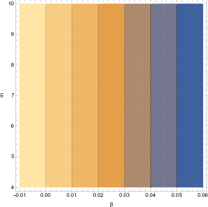
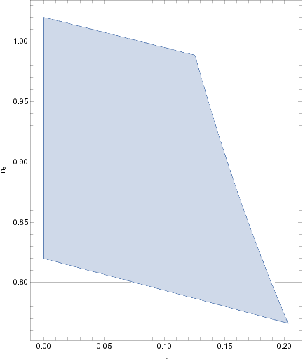
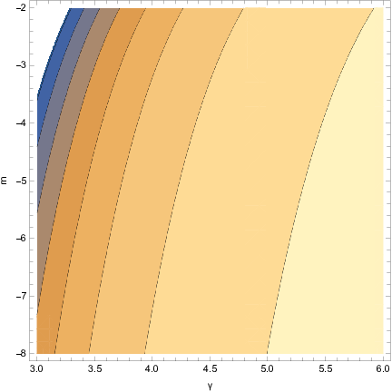
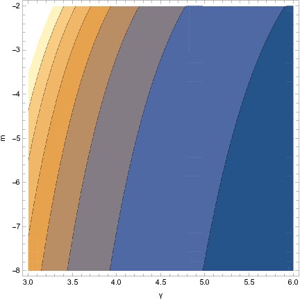
Assuming that in Planck Units, (, , ,
, , )=(1, , 60, 0, 0.013, 1) then
the resulting values for the spectral index of primordial
curvature perturbations and the tensor-to-scalar ratio are
and , which are are both compatible
results with the Planck 2018 data Akrami:2018odb.
Furthermore, the spectral index of tensor perturbations is
and the values of the scalar field are
and which indicates a decrease
in the scalar potential. And finally, when it comes to the
slow-roll indices, ,
,
. The effective value of
the last three is obviously zero.
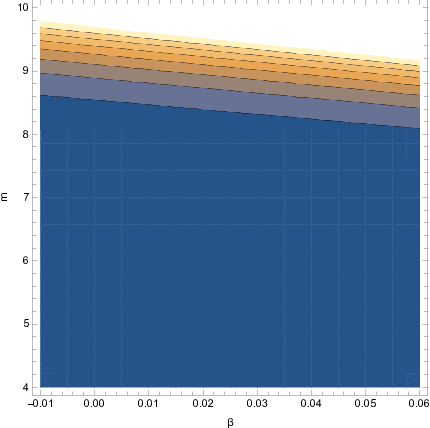
In addition, the predicted values for the non-Gaussianities are
also compatible results. We mention that the equilateral non
linear term obtains the value which is
quite a small value. Also, ,
, . The term
can obtain a greater value by decreasing , but such
decrease leads to a subsequent increase in the tensor-to-scalar
ratio so it must be made with care. Choosing leads
to while producing also viable spectral
indices and tensor-to-scalar ratio. Here, affects the
following quantities, the tensor-to-scalar ratio, the term
and the spectral index of scalar perturbations, but
mainly the first two, while the latter are affected greatly by the
constant-roll parameter .
Lastly, we examine the validity of our approximations. Concerning
the slow-roll approximations, we note that compared to
similarly
in contrast
to . Indeed, the approximations in
(6) are valid. Moreover, the string terms in the
equations of motion (3) and (4) are
and which justifies the reason the were
neglected. Also, the ratio is of order
. The term is of same order as
.
This set of values for the free parameters of the theory is
interesting due to the fact that selecting implies
that,
|
|
|
(94) |
which is an interesting relation between the scalar functions of the model.
VI Conclusions
In this work we investigated the quantitative effects of imposing
a constant-roll evolution on the scalar field for a
GW170817-compatible Einstein-Gauss-Bonnet theory. Our focus was on
the inflationary era, and we calculated the slow-roll indices and
the observational quantities of inflation, and we confronted
several models with the observational data coming from the Planck
2018 collaboration. As we demonstrated, the resulting inflationary
phenomenology can be compatible with the latest Planck data, for a
wide range of the free parameters of the theory, and with the
constant-roll condition holding true. In our calculations we
demonstrated that all the assumptions we made were satisfied for
all the models we examined, and for the values of the free
parameters that yield inflationary viability with respect to the
latest Planck data. For all the models we studied, we also
investigated the amount of non-Gaussianities that are predicted
from the models, by calculating the quantity in the
equilateral momentum approximation. Interestingly enough, we
demonstrated that the amount of non-Gaussianities is quite small
in the constant-roll case, and also in some cases, where we
compared the slow-roll and constant-roll cases explicitly, we
showed that the quantity is even smaller in the
constant-roll case, compared to the slow-roll case. Finally, we
performed an analytic approximation in the differential equation
that connects the scalar field potential and the scalar coupling
function, and we examined the phenomenology of inflation in this
case too. As we evinced, the model can also be compatible with the
Planck 2018 too.
A future study should address the important feature of having the
constraint holding true after the slow-roll or
constant-roll era, during the reheating era and beyond. In that
case, the differential equation that connects the scalar field
potential and the scalar coupling function
is not simplified, as it was during the inflationary era, thus one
may use the exact form of the differential equation, and impose
the constraint that it holds true for all the post-inflationary
eras, and that it exactly defines the interconnection of the
scalar potential and of the scalar-Gauss-Bonnet coupling. This
differential equation could be taken as an additional constraint
in the theory, and may affect the reheating era if the
constant-roll assumption is used, like for example in Ref.
Odintsov:2020sqy, or even if the slow-roll assumption is
used. The point is that in our previous work
Odintsov:2020sqy, and in the present work, we found only an
approximate relation for the scalar potential and the
scalar-Gauss-Bonnet coupling function, however, in the
post-inflationary era, the full differential equation should be
taken into account, and thus, one may have the exact relation
between the two scalar functions, without the need of any
approximation. Thus, one may use this differential equation as an
additional constraint, and solve thus numerically problems of
astrophysical or cosmological interest. This task is in our future
plans and we aim to materialize this in the next years, motivated
by the current astrophysical and cosmological interest on the
gravitational wave speed
Nair:2019iur; Carson:2020cqb; Giare:2020vss.