Hilbert-Schmidt speed as an efficient tool in quantum metrology

Hossein Rangani Jahromi Email: h.ranganijahromi@jahromu.ac.ir Affiliation: Physics Department, Faculty of Sciences, Jahrom University, P.B. 74135111, Jahrom, Iran Rosario Lo Franco Email: rosario.lofranco@unipa.it Affiliation: Dipartimento di Ingegneria, Università di Palermo, Viale delle Scienze, Edificio 6, 90128 Palermo, Italy

August 11, 2026

Abstract

We investigate how the Hilbert-Schmidt speed (HSS), a special type of quantum statistical speed, can be exploited as a powerful and easily computable tool for quantum phase estimation in a $n$ -qubit system. We find that, when both the HSS and quantum Fisher information (QFI) are computed with respect to the phase parameter encoded into the initial state of the $n$ -qubit register, the zeros of the HSS dynamics are essentially the same as those of the QFI dynamics. Moreover, the positivity (negativity) of the time-derivative of the HSS exactly coincides with the positivity (negativity) of the time-derivative of the QFI. Our results also provide strong evidence for contractivity of the HSS under memoryless dynamics and its sensitivity to system-environment information backflows to detect the non-Markovianity in high-dimensional systems, as predicted in previous studies.

Keywords:

Quantum Metrology, quantum Fisher information, Hilbert-Schmidt speed

I Introduction

When intending to estimate an unknown parameter in a quantum process, typically we prepare the probe system in an initial state, let it interact with an environment to encode the information about the unknown parameter, and then measure the probe to extract the information and estimate the parameter. It should be noted that in this process, the system also may be affected by different noises. Provided that the physical mechanism governing the system dynamics is known, we may deduce an estimated value of the parameter by comparison between the input and the output states of the probe Giovannetti et al. 2006.

Phase estimation is at the heart of quantum metrology Holevo 1978; Giovannetti et al. 2004; Paris 2009; Giovannetti et al. 2011; Liu et al. 2019; Tóth and Apellaniz 2014; Jafarzadeh et al. 2020; Rangani Jahromi 2020; Polino et al. 2020; Pirandola et al. 2018; Pezzè et al. 2018 such that in many technological areas, the estimation problem is concerned with determining a phase shift of the quantum state describing the probe. Estimation of an unknown phase has many significant applications such as the observation of gravitational waves Abbott et al. 2016 and detection of weak signals or defects resulting in the design of very sensitive sensors Taylor et al. 2013. In most of these scenarios an interferometric scheme is used to implement the quantum phase estimation. The most important variations of the interferometers include optical interferometry in gravitational wave detectors, Ramsey spectroscopy in atomic physics, optical imaging or laser gyroscopes to name but a few. All of these applications usually aim at optimal estimation of a relative phase gathered by one arm of the interferometer Dorner et al. 2009.

According to the quantum Cramér-Rao theorem, the precision of the quantum phase estimation is bounded by the inverse of the quantum Fisher information (QFI) Helstrom and Helstrom 1976; Paris 2009, which thus denotes a central quantity in quantum metrology. In fact, evaluation of the QFI provides the ultimate quantum limits to precision and consequently a general benchmark to assess quantum metrological protocols.

The QFI is also a measure of quantum statistical speed such that it quantifies the sensitivity of an initial state with respect to changes of the parameter which should be estimated. The more sensitivity indicates that the parameter, which could be an unknown phase shift of interest, can be estimated more efficiently, or with more precision. On the other hand, each measure of statistical distance naturally leads to a statistical speed for parametric evolutions of classical probability distributions or quantum states. This statistical speed can be obtained by the change in distance originated from a small change of this parameter (i.e., the derivative of the distance). The quantum statistical speed is obtained by maximizing over the classical statistical speed over all quantum measurements Gessner and Smerzi 2018.

Inspired by the fact that the QFI can be derived as quantum statistical speed from the Hellinger distance Jeffreys 1946, we investigate the application of the Hilbert-Schmidt speed (HSS), another interesting quantifier of quantum statistical speed which has the advantage of avoiding diagonalization of the evolved density matrix, in the quantum phase estimation. Because the computation of the QFI for high-dimensional quantum systems is very complicated, it would be useful to inquire the efficiency of the HSS, which is an easily computable quantity, in the quantum estimation theory.

In this paper, we show that the HSS can be exploited as a powerful and convenient figure of merit in quantum metrology for $n$ -qubit systems. This result gains particular attention considering the fact that most of the quantum information protocols are designed by $n$ -qubit registers.

The paper is organized as follows. In Sec. II we briefly review the definition of the QFI and HSS. In Sec. III we present our main result about the applicability of the HSS in quantum phase estimation and check its validity by various examples. Finally, Sec. IV summarizes the main results and prospects.

II Preliminaries

II.1 Quantum Fisher information (QFI)

We start by recalling the general formulation resulting in defining a kind of quantum statistical speed by which the QFI can be characterized.

First, we consider the (classical) Hellinger distance Jeffreys 1946

[d(p,q)]^{2}=\dfrac{1}{2}\sum\limits_{x}|\sqrt{p_{x}}-\sqrt{q_{x}}|^{2},

(1)

in which $p=\{p_{x}\}_{x}$ and $q=\{q_{x}\}_{x}$ represent the probability distributions. Here it has been assumed that the random variable $x$ takes only discrete values.

Formally, in order to achieve the statistical speed from a given statistical distance, one should quantify the distance between infinitesimally close distributions taken from a one-parameter family $p_{x}(\varphi)$ with parameter $\varphi$ . Following this prescription and performing a Taylor expansion at $\varphi_{0}$ for small values of $\varphi$ , we find that the classical statistical speed associated with the (classical) Hellinger distance is given by

s[p(\varphi_{0})]\equiv\dfrac{d}{d\varphi}d\big(p(\varphi_{0}+\varphi),p(\varphi_{0})\big)=\sqrt{\dfrac{f(p(\varphi_{0}))}{8}},

(2)

where

f(p(\varphi))=\sum_{x}p_{x}(\varphi)\bigg(\dfrac{\partial~\text{ln}p_{x}(\varphi)}{\partial\varphi}\bigg)^{2},

(3)

denotes the Fisher information Braunstein and Caves 1994; Paris 2009.

Extending these classical notions to the quantum case with considering a given pair of quantum states $\rho$ and $\sigma$ , one may write $p_{x}=\text{Tr}\{E_{x}\rho\}$ and $q_{x}=\text{Tr}\{E_{x}\sigma\}$ representing the measurement probabilities associated with the positive-operator-valued measure (POVM) defined by the $\{E_{x}\geq 0\}$ which satisfies $\sum\limits_{x}E_{x}=\mathbb{I}$ . The associated quantum distance can be obtained by maximizing the classical distance over all possible choices of POVMs Luo and Zhang 2004, i.e.,

D(\rho,\sigma)=\max_{\{E_{x}\}}d(p,q)=\sqrt{1-\mathcal{F}(\rho,\sigma)},

(4)

called the Bures distance Braunstein and Caves 1994 in which $\mathcal{F}(\rho,\sigma)\equiv\text{Tr}\sqrt{\sqrt{\rho}\sigma\sqrt{\rho}}$ denotes the fidelity Jozsa 1994.

Now we can define the quantum statistical speed Braunstein and Caves 1994 as follows

S[\rho(\varphi_{0})]\equiv\dfrac{d}{d\varphi}D\big(\rho(\varphi_{0}+\varphi),\rho(\varphi_{0})\big)=\sqrt{\dfrac{F(\rho(\varphi_{0}))}{8}},

(5)

where the quantum Fisher information (QFI) is given by Braunstein and Caves 1994; Giovannetti et al. 2006; Giovannetti et al. 2011; Liu et al. 2019

	$\displaystyle F(\rho(\varphi))\equiv F_{\varphi}=\sum_{i,j}\frac{2}{\lambda_{i}+\lambda_{j}}\|\langle\phi_{i}\|\partial_{\varphi}\rho\left(\varphi\right)\|\phi_{j}\rangle\|^{2}~~~~~~~~~~~~~~~~~$
	$\displaystyle\ =\sum_{i}\frac{(\partial_{\varphi}\lambda_{i})^{2}}{\lambda_{i}}+2\sum_{i\neq j}\frac{(\lambda_{i}-\lambda_{j})^{2}}{\lambda_{i}+\lambda_{j}}\|\langle\phi_{i}\|\partial_{\varphi}\phi_{j}\rangle\|^{2},$		(6)

in which $|\phi_{i}\rangle$ and $\lambda_{i}$ , respectively, denote the eigenvectors and eigenvalues of matrix $\rho\left(\varphi\right)$ . In fact, the QFI is obtained by maximizing the Fisher information over all possible POVMs Paris 2009, i.e.,

F(\rho(\varphi))=\max_{\{E_{x}\}}f(p(\varphi)),

(7)

in which $p(\varphi)=\{p_{x}(\varphi)\}_{x}$ and $p_{x}(\varphi)=\text{Tr}\{E_{x}\rho(\varphi)\}$ . The fundamental relationship between the QFI and its corresponding quantum bound is expressed by the quantum Cramér-Rao bound stating that Braunstein and Caves 1994

\Delta\varphi_{QCR}=\sqrt{\dfrac{1}{F(\rho(\varphi))}},

(8)

setting the precision limit for quantum estimation of unknown parameter $\varphi$ .

II.2 Hilbert-Schmidt speed (HSS)

Introducing the distance measure Gessner and Smerzi 2018

[\text{d}(p,q)]^{2}=\dfrac{1}{2}\sum\limits_{x}|p_{x}-q_{x}|^{2},

(9)

in which $p=\{p_{x}\}_{x}$ as well as $q=\{q_{x}\}_{x}$ are probability distributions, and subsequently considering the classical statistical speed

\text{s}\big[p(\varphi_{0})\big]=\dfrac{d}{d\varphi}\text{d}\big(p(\varphi_{0}+\varphi),p(\varphi_{0})\big),

(10)

we can define a special kind of quantum statistical speed which is called the HSS. Following the procedure discussed in the previous subsection for obtaining the corresponding quantum relations, one may obtain the Hilbert-Schmidt distance Ozawa 2000

\text{D}(\rho,\sigma)\equiv\max_{\{E_{x}\}}\text{d}(\rho,\sigma)=\sqrt{\frac{1}{2}\text{Tr}[(\rho-\sigma)^{2}]},

(11)

not requiring the diagonalization of the argument operator. Moreover, the corresponding quantum statistical speed also called the HSS, is obtained as follows Gessner and Smerzi 2018

	$\displaystyle HSS\bigg(\rho(\varphi)\bigg)\equiv HSS_{\varphi}$	$\displaystyle\equiv\text{S}\big[\rho(\varphi)\big]=\max_{\{E_{x}\}}\text{s}\big[p(\varphi)\big]$
		$\displaystyle=\sqrt{\frac{1}{2}\text{Tr}\bigg[\bigg(\dfrac{d\rho(\varphi)}{d\varphi}\bigg)^{2}\bigg]},$		(12)

which can be computed without diagonalizing $\text{d}\rho(\varphi)/\text{d}\varphi$ .

III Quantum estimation through HSS

Because both the QFI and HSS are quantum statistical speeds associated, respectively, with the Bures and Hilbert-Schmidt distances, it is reasonable to investigate how they can be related to each other. By numerical simulation, we find that there is an important relationship between them. We state it in the following.

Main Result.

Suppose that we are given a pure initial state of a $n$ -qubit quantum register, i.e.,

|\psi_{0}\rangle=N\sum_{j}\text{e}^{i\varphi_{j}}c_{j}|j\rangle

(13)

in which $N=\frac{1}{\sqrt{\sum_{j}|c_{j}|^{2}}}$ represents the normalization factor and $\left\{|j\rangle\right\}$ denotes the computational basis. Then, this state is affected by a general quantum channel $\mathcal{E}_{t}$ such that the output state is given by $\rho_{t}=\mathcal{E}_{t}(|\psi_{0}\rangle\langle\psi_{0}|)$ . Under these conditions, we find that $HSS_{\varphi_{j}}\equiv HSS\bigg(\rho_{t}(\varphi_{j})\bigg)$ and $F_{\varphi_{j}}\equiv F\bigg(\rho_{t}(\varphi_{j})\bigg)$ computed with respect to phase parameter $\varphi_{j}$ encoded into the input state (13), exhibit qualitatively the same dynamics such that if $HSS_{\varphi_{j}}\neq 0$ , we have $\dfrac{\text{d}HSS_{\varphi_{j}}}{\text{d}t}\geq 0\Leftrightarrow\dfrac{\text{d}F_{\varphi_{j}}}{\text{d}t}\geq 0$ and $\dfrac{\text{d}HSS_{\varphi_{j}}}{\text{d}t}\leq 0\Leftrightarrow\dfrac{\text{d}F_{\varphi_{j}}}{\text{d}t}\leq 0$ . Moreover, $HSS_{\varphi_{j}}=0\Leftrightarrow F_{\varphi_{j}}=0$ . Therefore, investigating the HSS dynamics, we can detect the instants at which the optimal phase estimation is achieved.

The sanity check of this technique is performed by presenting various examples in the following subsections. It should be noted that using the general hierarchy between the HSS and QFI discussed in Gessner and Smerzi 2018, one can show that $0\leqslant HSS_{\varphi_{j}}\leqslant\sqrt{F_{\varphi_{j}}}$ , hence $F_{\varphi_{j}}=0$ leads to $HSS_{\varphi_{j}}$ . However, the reverse (i.e., detecting the QFI zeros through the HSS zeros, which we discussed in this paper) cannot be necessarily extracted from the above general inequality.

III.1 One-qubit example

First we focus on a one-qubit system interacting with a dissipative reservoir through the Hamiltonian

H=\omega_{0}~\sigma_{+}\sigma_{-}+\sum\limits_{k}\omega_{k}b^{\dagger}_{k}b_{k}+(\sigma_{+}B+\sigma_{-}B^{\dagger}),

(14)

where $\omega_{0}$ denotes the transition frequency of the qubit, $\sigma_{\pm}$ represent the system raising and lowering operators, $\omega_{k}$ is the frequency of the $k$ -th field mode of the reservoir, $b_{k}$ ( $b^{\dagger}_{k}$ ) denotes the $k$ -mode annihilation (creation) operator, and $B=\sum_{k}g_{k}b_{k}$ in which $g_{k}$ represents the coupling constant with the $k$ -th mode.

At zero temperature and in the strong-coupling regime using Hamiltonian (14) with a Lorentzian spectral density for the cavity modes and preparing the qubit in initial state

|\psi_{0}\rangle=\text{cos}(\theta)|1\rangle+\text{e}^{i\varphi}\text{sin}(\theta)|0\rangle,

(15)

one can find that the dynamics of the qubit in basis $\{|1\rangle,~|0\rangle\}$ is described by the following evolved reduced density matrix Breuer et al. 2002; Bellomo et al. 2007

\rho^{S}(t)=\left(\begin{array}[]{cc}\dfrac{P_{t}}{2}\left(\cos\left(\theta\right)+1\right)&\dfrac{\sqrt{P_{t}}}{2}{{\rm e}^{-i\varphi}}\sin\left(\theta\right)\\ \vskip 6.0pt plus 2.0pt minus 2.0pt\cr\dfrac{\sqrt{P_{t}}}{2}{{\rm e}^{i\varphi}}\sin\left(\theta\right)&1-\dfrac{P_{t}}{2}\left(\cos\left(\theta\right)+1\right)\end{array}\right),

(16)

in which the coherence characteristic function $P(t)$ is

P(t)=\text{e}^{-\lambda t}\left[\cos(\Gamma t/2)+(\lambda/\Gamma)\sin(\Gamma t/2)\right]^{2},

(17)

with $\Gamma=\sqrt{2\gamma_{0}\lambda-\lambda^{2}}$ . The parameter $\lambda$ , connected to the reservoir correlation time $\tau_{c}$ by relation $\tau_{c}\approx 1/\lambda$ , represents the spectral width for the qubit-reservoir coupling. Moreover, decay rate $\gamma_{0}$ is related to the system (qubit) relaxation time scale $\tau_{r}$ , over which the state of the system changes, by relation $\tau_{r}=1/\gamma_{0}$ .

Inserting (16) into Eqs. (II.1) and (II.2), we find that the QFI and HSS associated with initial phase $\varphi$ , respectively, are given by

F_{\varphi}(t)=P_{t}\sin^{2}\left(\theta\right),

(18)

and

HSS_{\varphi}(t)=\dfrac{\sqrt{P_{t}}}{2}\sin\left(\theta\right),

(19)

leading to relations

F_{\varphi}=4(HSS_{\varphi})^{2}\Longrightarrow\dfrac{\text{d}F_{\varphi}}{\text{d}t}=(8~HSS_{\varphi})\dfrac{\text{d}HSS_{\varphi}}{\text{d}t}.

(20)

Accordingly, we see that when the HSS vanishes, the QFI also equals zero. Moreover, at all instances when $HSS_{\varphi}\neq 0$ , the signs of $\dfrac{\text{d}F_{\varphi}}{\text{d}t}$ and $\dfrac{\text{d}HSS_{\varphi}}{\text{d}t}$ are similar and hence they exhibit qualitatively the same dynamics. In particular, the times at which the optimal estimation is achieved, i.e., $\dfrac{\text{d}F_{\varphi}}{\text{d}t}=0$ , can be easily detected by investigating the HSS dynamics.

III.2 Two-qubit examples

Here the validity of our result for two-qubit systems in three different scenarios, i.e., coupling to independent environments, interaction with common environment, and teleportation of the entanglement between the qubits, is discussed.

III.2.1 Coupling to independent environments

We now study a composite quantum system which consists of two separated qubits independently interacting with their own dissipative reservoir. Knowing the evolved density matrix of the single qubit discussed in previous subsection, one can easily obtain the density matrix evolution of the two independent qubits Bellomo et al. 2007. We investigate the scenario in which the two qubits are prepared in initial state

|\psi_{0}\rangle=\frac{1}{\sqrt{3}}(\text{e}^{i\varphi}|10\rangle+|01\rangle+|00\rangle),

(21)

resulting in the evolved reduced density matrix

\rho^{S}(t)=\left(\begin{array}[]{cccc}0&0&0&0\\ 0&\dfrac{P_{t}}{3}&\dfrac{P_{t}}{3}e^{i\varphi}&\dfrac{\sqrt{P_{t}}}{3}e^{i\varphi}\\ 0&\dfrac{P_{t}}{3}e^{-i\varphi}&\dfrac{P_{t}}{3}&\dfrac{\sqrt{P_{t}}}{3}\\ 0&\dfrac{\sqrt{P_{t}}}{3}e^{-i\varphi}&\dfrac{\sqrt{P_{t}}}{3}&1-\dfrac{2P_{t}}{3}\\ \end{array}\right),

(22)

where $P_{t}\in[0,1]$ is the coherence characteristic function of Eq. (17). Computing the QFI and HSS with respect to phase parameter $\varphi$ , one promptly gets that they are given, respectively, by

F_{\varphi}(t)=\dfrac{8}{9}P_{t},\quad HSS_{\varphi}(t)=\frac{1}{3}\sqrt{P_{t}(P_{t}+1)}.

(23)

resulting in

	$\displaystyle F_{\varphi}$	$\displaystyle=$	$\displaystyle\dfrac{4}{9}(\,\sqrt{1+36\,{{\it HSS^{2}_{\varphi}}}}-1)\Rightarrow$
	$\displaystyle\dfrac{\text{d}F_{\varphi}}{\text{d}t}$	$\displaystyle=$	$\displaystyle{\frac{{\it 16~HSS_{\varphi}}}{\sqrt{1+36\,{{\it HSS^{2}_{\varphi}}}}}}\dfrac{\text{d}HSS_{\varphi}}{\text{d}t}.$		(24)

Again assuming that $HSS_{\varphi_{j}}\neq 0$ , we have $\dfrac{\text{d}HSS_{\varphi_{j}}}{\text{d}t}\geq 0\Leftrightarrow\dfrac{\text{d}F_{\varphi_{j}}}{\text{d}t}\geq 0$ and $\dfrac{\text{d}HSS_{\varphi_{j}}}{\text{d}t}\leq 0\Leftrightarrow\dfrac{\text{d}F_{\varphi_{j}}}{\text{d}t}\leq 0$ . In addition, at instants when $HSS_{\varphi_{j}}=0$ , the QFI also vanishes and hence no information can be extracted from the system.

III.2.2 Interaction with common environment

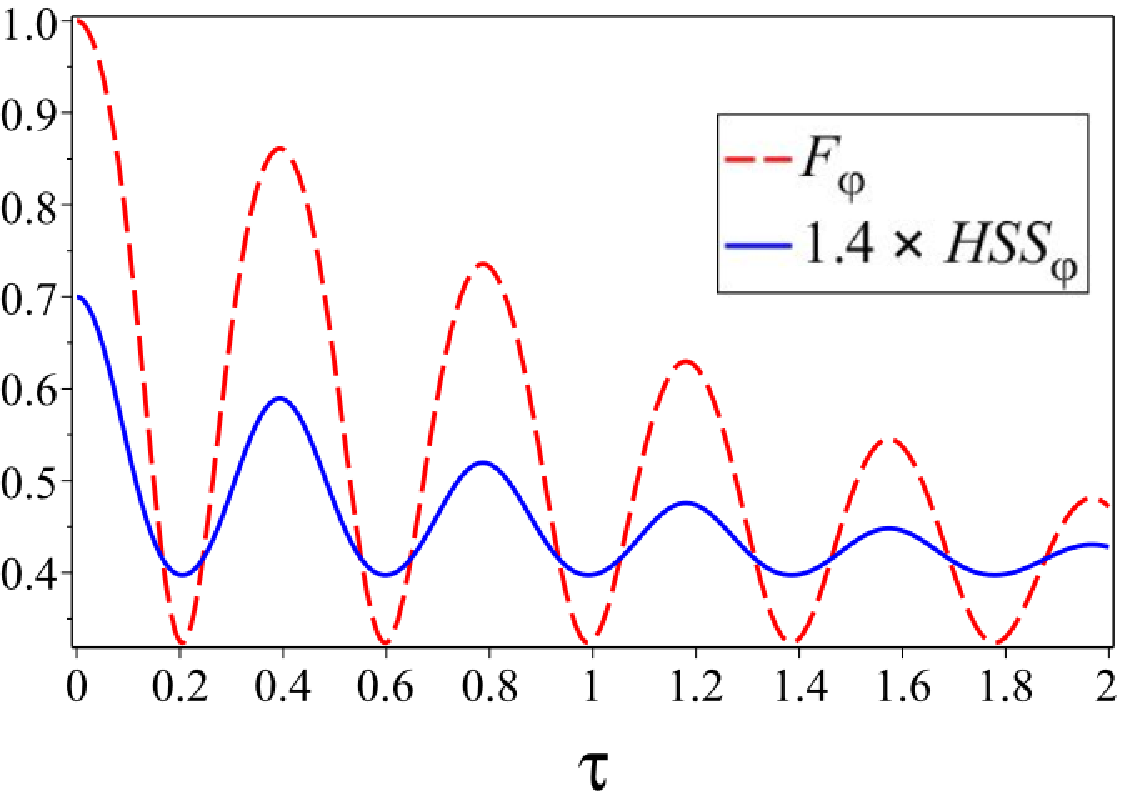
Refer to caption — Figure 1: Dynamics of quantum Fisher information $F_{\varphi}(t)$ (red dashed line) and Hilbert-Schmidt speed $HSS_{\varphi}(t)$ (amplified by $1.4$ times for comparison, blue solid line), as a function of the dimensionless time $\tau$ for the two-qubits system coupled to a common reservoir, with $r_{1}=0.3$ and $R=8$ .

We study two qubits interacting with a common zero-temperature bosonic reservoir. The total Hamiltonian of the two-qubit system plus the reservoir is written as $H=H_{0}+H_{int}$ , with Maniscalco et al. 2008

	$\displaystyle H_{0}$	$\displaystyle=$	$\displaystyle\omega_{1}~\sigma^{(1)}_{+}\sigma^{(1)}_{-}+\omega_{2}~\sigma^{(2)}_{+}\sigma^{(2)}_{-}+\sum\limits_{k}\omega_{k}b^{\dagger}_{k}b_{k},$
	$\displaystyle H_{\mathrm{int}}$	$\displaystyle=$	$\displaystyle(\alpha_{1}\sigma^{(1)}_{+}+\alpha_{2}\sigma^{(2)}_{+})B+(\alpha_{1}\sigma^{(1)}_{-}+\alpha_{2}\sigma^{(2)}_{-})B^{\dagger},$		(25)

where $\sigma^{(j)}_{\pm}$ and $\omega_{j}$ denote, respectively, the inversion operator and transition frequency of the $j$ th qubit, $j=1,2$ , $b^{\dagger}_{k}$ ( $b_{k}$ ) represents the $k$ -mode creation (annihilation) operator of quanta of the environment, and $B=\sum_{k}g_{k}b_{k}$ in which $g_{k}$ is the coupling constant with the $k$ -th mode. Moreover, the interaction of the $j$ th qubit with the reservoir is measured by the dimensionless constant $\alpha_{j}$ depending on the value of the cavity field at the qubit position and can be effectively controlled by means of dc Stark shifts tuning the atomic transition in and out of the resonance. We investigate the case in which the two atomic qubits interact resonantly with the reservoir described by a Lorentzian spectral density and they have the same transition frequency, i.e., $\omega_{1}=\omega_{2}=\omega_{0}$ .

It is useful to introduce a collective coupling constant $\alpha_{T}=\sqrt{\alpha^{2}_{1}+\alpha^{2}_{2}}$ , the relative strengths $r_{j}=\alpha_{j}/\alpha_{T}$ such that $r_{1}^{2}+r_{2}^{2}=1$ , and mutually orthogonal quantum states

|\psi_{+}\rangle=r_{1}|10\rangle+r_{2}|01\rangle,\quad|\psi_{-}\rangle=r_{2}|10\rangle-r_{1}|01\rangle.

(26)

With these definitions, one finds that for an initial state of the form

|\psi_{0}\rangle=\big[\dfrac{1}{\sqrt{2}}(|10\rangle+\text{e}^{i\varphi}|01\rangle)\big]\bigotimes_{k}|0_{k}\rangle,

(27)

and in the basis $\{|1\rangle,|0\rangle\}$ , the reduced density operator for the the two-qubit system is written as Maniscalco et al. 2008

\rho(t)=\left(\begin{array}[]{cccc}0&0&0&0\\ 0&|c_{1}(t)|^{2}&c_{1}(t)c^{*}_{2}(t)&0\\ 0&c^{*}_{1}(t)c_{2}(t)&|c_{2}(t)|^{2}&0\\ 0&0&0&1-|c_{1}(t)|^{2}-|c_{2}(t)|^{2}\\ \end{array}\right),

(28)

where, considering $\beta_{\pm}=\langle\psi_{\pm}|\psi_{0}\rangle$ , one has

c_{1}(t)=r_{2}\beta_{-}+r_{1}\mathcal{F}_{t}\beta_{+},\quad c_{2}(t)=-r_{1}\beta_{-}+r_{2}\mathcal{F}_{t}\beta_{+}.

(29)

Moreover, defining dimensionless quantities $\tau=\lambda t$ and $R=\mathcal{R}/\lambda$ in which $1/\lambda$ is the reservoir correlation time and $\mathcal{R}$ denotes the vacuum Rabi frequency, we have

\mathcal{F}_{\tau}=\text{e}^{-\tau/2}\left[\cosh(\frac{\tau}{2}\sqrt{1-4R^{2}})+\dfrac{1}{\sqrt{1-4R^{2}}}\sinh(\frac{\tau}{2}\sqrt{1-4R^{2}})\right].

(30)

The QFI can be computed analytically, however it is too complicated to present here. On the other hand, we find that the HSS is given by

HSS_{\varphi}(t)=\dfrac{1}{2}\left({r_{{1}}}^{2}+{r_{{2}}}^{2}\right)\sqrt{{\mathcal{F}_{t}}^{2}{r_{{1}}}^{4}-2\,\left({\mathcal{F}_{t}}^{2}-1\right)^{2}{r_{{1}}}^{2}{r_{{2}}}^{2}\cos\left(2\,\varphi\right)+2\,\left({\mathcal{F}_{t}}^{4}-{\mathcal{F}_{t}}^{2}+1\right){r_{{1}}}^{2}{r_{{2}}}^{2}+{\mathcal{F}_{t}}^{2}{r_{{2}}}^{4}}.

(31)

Figure 1 illustrates that the QFI and HSS dynamics simultaneously exhibit an oscillatory behavior such that their maximum and minimum points exactly coincide. This figure qualitatively verifies our result that the HSS can detect exactly the times at which the best phase estimation occurs. In fact, the HSS, similar to QFI, can be used as a distinguishability metric on the space of quantum states which quantifies the maximum amount of information on an unknown phase parameter attainable by a given probe state.

III.2.3 Two-qubit teleportation

One of the most important models used in the low-temperature regime is typically the spin environment Rangani Jahromi et al. 2019; Lombardo and Villar 2010. In particular, in order to achieve the proper operation in experiments performed to study the macroscopic quantum coherence and decoherence, one require temperatures close to absolute zero. Here we consider a two-qubit system interacting with an external environment composed of $N$ spins. The general Hamiltonian is therefore written as $H=H_{S}+H_{E}+H_{I}$ where the system, environment and interaction Hamiltonians, respectively, are given by

H_{S}=\dfrac{\hbar\Omega_{1}}{2}\sigma_{z}^{1}+\dfrac{\hbar\Omega_{2}}{2}\sigma_{z}^{2}+\gamma\sigma_{z}^{1}\sigma_{z}^{2},

(32)

H_{E}=\sum\limits_{i=1}^{N}h_{i}\sigma_{xi},

(33)

H_{I}=\sigma_{z}^{1}\otimes\sum\limits_{n=1}^{N}\varepsilon_{i}\sigma_{zi}+\sigma_{z}^{2}\otimes\sum\limits_{n=1}^{N}\lambda_{i}\sigma_{zi},

(34)

in which $\Omega_{i}$ and $\gamma$ denote, respectively, the characteristic frequency of $i$ th qubit, and the coupling strength between the two spin qubits. Moreover, $\xi_{i}$ ( $\lambda_{i}$ ) represents the coupling between qubit 1 ( qubit 2) and the spins of the environment, and $h_{i}$ denotes the tunneling matrix element for the $i$ th-environmental spin.

Preparing the two-qubit system in initial state

\rho(0)=\frac{1-r}{4}\mathcal{I}+r|\vartheta\rangle\langle\vartheta|

(35)

where $r\in(0,1]$ denotes the mixing of the state, $\mathcal{I}$ is $4\times 4$ unity operator and

|\vartheta\rangle=\sqrt{1-p}|00\rangle+\sqrt{p}|11\rangle;~~0\leq p\leq 1,

(36)

one finds that the evolved reduced density matrix is given by Lombardo and Villar 2010

\rho(t)=\left(\begin{array}[]{cccc}\dfrac{1-r}{4}+r(1-p)&0&0&r\sqrt{p(1-p)}e^{-i(\Omega_{1}+\Omega_{2})t}Q(t)\\ 0&\dfrac{1-r}{4}&0&0\\ 0&0&\dfrac{1-r}{4}&0\\ r\sqrt{p(1-p)}e^{i(\Omega_{1}+\Omega_{2})t}Q(t)&0&0&\dfrac{1-r}{4}+rp\\ \end{array}\right),

(37)

where the decoherence factor $Q(t)$ is

Q(t)=\prod\limits_{i=1}^{N}\bigg\lgroup 1-\big[\dfrac{2(\varepsilon_{i}+\lambda_{i})^{2}}{h_{i}^{2}+(\varepsilon_{i}+\lambda_{i})^{2}}\big]\text{sin}^{2}(t\sqrt{h_{i}^{2}+(\varepsilon_{i}+\lambda_{i})^{2}})\bigg\rgroup.

(38)

Assuming that the two qubits are shared between Alice and Bob, we use two copies of this system as a resource for teleportation of an unknown entangled state $\rho_{in}$ . It is useful to introduce the Bell states $\mathcal{B}_{i}$ ’s associated with the Pauli matrices $\sigma_{i}$ ’s by

\mathcal{B}_{i}=\left(\sigma_{0}\otimes\sigma_{i}\right)\mathcal{B}_{0}\left(\sigma_{0}\otimes\sigma_{i}\right);\;i=1,2,3,

(39)

in which $\sigma_{0}=I$ , $\sigma_{1}=\sigma_{x}$ , $\sigma_{2}=\sigma_{y}$ , $\sigma_{3}=\sigma_{z}$ , and $I$ represents the $2\times 2$ identity matrix. In addition, we choose $\mathcal{B}_{0}=\frac{1}{2}\left(\Ket{00}+\Ket{11}\right)\left(\Bra{00}+\Bra{11}\right)$ where $\left\{\Ket{0},\Ket{1}\right\}$ is the usual computational basis for the one-qubit system. Now, following Lee and Kim 2000, one can generalize the standard teleportation protocol $T_{0}$ and find that the output state of the two-qubit teleportation is given by Bowen and Bose 2001

\rho_{\text{out}}=\sum_{ij}p_{ij}\left(\sigma_{i}\otimes\sigma_{j}\right)\rho_{\text{in}}\left(\sigma_{i}\otimes\sigma_{j}\right),\ i,j=0,x,y,z,

(40)

where $p_{ij}=\text{Tr}\left(\mathcal{B}_{i}\rho_{\text{res}}\right)\text{Tr}\left(\mathcal{B}_{j}\rho_{\text{res}}\right)$ in which $\rho_{\text{res}}$ , the resource state for the teleportation, equals the reduced density matrix (37) in our model. Accordingly, for the input state $\rho_{in}=\Ket{\psi_{in}}\Bra{\psi_{in}}$ with

\Ket{\psi_{in}}=\text{cos}(\theta/2)\Ket{10}+\text{sin}(\theta/2)\text{e}^{i\varphi}\Ket{01},

(41)

where $\ 0\leq\theta\leq\pi,\ 0\leq\varphi\leq 2\pi$ , we find that the output state of the teleportation can be written as

\rho_{out}(t)=\left[\begin{array}[]{cccc}4\,{R}^{2}+2\,Rr&0&0&0\\ \vskip 6.0pt plus 2.0pt minus 2.0pt\cr 0&\left(4\,Rr+{r}^{2}\right)\sin^{2}\left(\dfrac{\theta}{2}\right)+4\,{R}^{2}&2\,{e}^{i\varphi}\sin\left(\theta\right){A^{2}(t)}\cos^{2}\big(\Omega_{{1}}+\Omega_{{2}}\big)&0\\ \vskip 6.0pt plus 2.0pt minus 2.0pt\cr 0&2\,{e}^{-i\varphi}\sin\left(\theta\right){A^{2}(t)}\cos^{2}\big(\Omega_{{1}}+\Omega_{{2}}\big)&\left(4\,Rr+{r}^{2}\right)\cos^{2}\left(\dfrac{\theta}{2}\right)+4\,{R}^{2}&0\\ \vskip 6.0pt plus 2.0pt minus 2.0pt\cr 0&0&0&4\,{R}^{2}+2\,Rr\end{array}\right],

(42)

in which $R=\dfrac{1-r}{4}$ and $A(t)=\sqrt{\left(1-p\right)p}rQ(t)$ . Using this expression for the output state, we find that the QFI and HSS associated to the phase parameter encoded into the input state used in teleportation channel are given, respectively, by

F_{\varphi}(t)=32\,{\frac{{A}^{4}(t)\cos^{4}\big(\Omega_{{1}}+\Omega_{{2}}\big)\sin^{2}\theta}{1+{r}^{2}}},

(43)

HSS_{\varphi}(t)=2\,{A}^{2}(t)\cos^{2}\big(\Omega_{{1}}+\Omega_{{2}}\big)\sin\theta.

(44)

Therefore, we obtain

F_{\varphi}={\frac{{{\it 8~HSS^{2}_{\varphi}}}}{1+{r}^{2}}}\Longrightarrow\dfrac{\text{d}F_{\varphi}}{\text{d}t}={\frac{{{\it 16~HSS_{\varphi}}}}{1+{r}^{2}}}\dfrac{\text{d}HSS_{\varphi}}{\text{d}t},

(45)

leading to our main result, i.e., the possibility of extracting the QFI dynamics through the HSS dynamics.

III.3 $n$ -qubit example ( $n\geq 3$ )

First we consider the dynamics of a topological qubit realized by two Majorana modes which are generated at the endpoints of some nanowire with strong spin-orbit interaction, placed on top of an s-wave superconductor and driven by an external magnetic field B along the wire axis direction Ho et al. 2014; Rangani Jahromi and Haseli 2020. We also assume that each Majorana mode is coupled to the metallic nanowire via a tunnel junction in the way that the tunneling strength is controllable by an external gate voltage.

The total Hamiltonian is written as

H=H_{S}+H_{E}+V

(46)

in which $H_{s}$ denotes the Hamiltonian of the topological qubit and $V$ represents the system-environment interaction Hamiltonian. In addition, the environment Hamiltonian is denoted by $H_{E}$ whose elementary constituents can be considered as electrons or holes. The decoherence which affects the topological qubit is modelled as a fermionic Ohmic-like environment described by spectral density $\rho_{spec}\propto\omega^{Q}$ with $Q\geq 0$ . The Ohmic, supere Ohmic and sub-Ohmic environments are characterized by $Q=1$ , $Q>1$ and $Q<1$ , respectively.

Since these Majorana modes used as the topological qubit are zero-energy modes, we have $H_{S}=0$ . Moreover, interaction Hamiltonian $V$ constructed by the electron creation (annihilation) operators with Majorana modes $\gamma_{1}$ and $\gamma_{2}$ satisfies the properties:

\gamma^{\dagger}_{a}=\gamma_{a},~~~\{\gamma_{a},\gamma_{b}\}=2\delta_{ab},

(47)

where $a,b=1,2$ . Before turning on interaction $V$ , the two Majorana modes construct a topological (non-local) qubit with states $|0\rangle$ and $|1\rangle$ related to each other by

\frac{1}{2}(\gamma_{1}-\text{i}\gamma_{2})|0\rangle=|1\rangle,~~~~~\frac{1}{2}(\gamma_{1}+\text{i}\gamma_{2})|1\rangle=|0\rangle,

(48)

where the following representation has been chosen for $\gamma_{1,2}$ :

\gamma_{1}=\sigma_{1},~~~\gamma_{2}=\sigma_{2},~~~\text{i}\gamma_{1}\gamma_{2}=\sigma_{3},

(49)

in which $\sigma_{j}$ ’s represent the Pauli matrices.

Assuming that $\varrho^{T}$ , denoting the state of the total system, is uncorrelated initially: $\varrho^{T}(0)=\varrho(0)\otimes\varrho_{E}$ , in which $\rho_{S}(0)$ and $\rho_{E}$ are the initial density matrices of the topological qubit and its environment, respectively. Supposing that the initial state of the Majorana qubit is written as

\varrho(0)=\left(\begin{array}[]{cc}\varrho_{11}(0)&\varrho_{12}(0)\\ \varrho_{21}(0)&\varrho_{22}(0)\\ \end{array}\right),

(50)

one finds that the reduced density matrix of the system at time $t$ can be obtained by dynamical map $\Phi_{t}$ such that (for details, see Ho et al. 2014):

	$\displaystyle\varrho(t)$	$\displaystyle=\Phi_{t}\big(\varrho(0)\big)=$
		$\displaystyle\frac{1}{2}\left(\begin{array}[]{cc}1+(2\varrho_{11}(0)-1)\alpha^{2}(t)&2\varrho_{12}(0)\alpha(t)\\ 2\varrho_{21}(0)\alpha(t)&1+(2\varrho_{22}(0)-1)\alpha^{2}(t)\\ \end{array}\right),$

in which

\alpha(t)=\text{e}^{-2B^{2}|\beta|I_{Q}(t)},~~~~~\beta\equiv\dfrac{-4\pi}{\Gamma(Q+1)}(\dfrac{1}{\varGamma_{0}})^{Q+1}

(53)

where $\varGamma_{0}$ denotes the high-frequency cutoff for the linear spectrum of the edge state and $\Gamma(z)$ represents the Gamma function. In addition,

I_{Q}(t)=\left\{\begin{array}[]{rl}2\varGamma_{0}^{Q-1}\Gamma(\frac{Q-1}{2})\bigg[1-\,_{1}F_{1}\big(\frac{Q-1}{2};\frac{1}{2};-\frac{t^{2}\varGamma^{2}_{0}}{4}\big)\bigg],&Q\neq 1,\\ \frac{1}{2}t^{2}\varGamma^{2}_{0}\,{}_{2}F_{2}\bigg(\{1,1\};\{3/2,2\};-\frac{t^{2}\varGamma^{2}_{0}}{4}\bigg),&Q=1,\end{array}\right.

(54)

where ${}_{p}F_{q}$ is the generalized hypergeometric function and $\varGamma(z)$ denotes the Gamma function.

From the eigenvalues and eigenvectors of the Choi matrix Leung 2003 of the map $\Phi_{t}$ , the corresponding Kraus operators $\{K_{i}(t)\}$ can be obtained as

		$\displaystyle K_{1}(t)=\left(\begin{array}[]{cc}\frac{\alpha-1}{2}&0\\ 0&\frac{1-\alpha}{2}\\ \end{array}\right),~K_{2}(t)=\left(\begin{array}[]{cc}\frac{\alpha+1}{2}&0\\ 0&\frac{\alpha+1}{2}\\ \end{array}\right),$
		$\displaystyle K_{3}(t)=\left(\begin{array}[]{cc}0&\frac{\sqrt{1-\alpha^{2}}}{\sqrt{2}}\\ 0&0\\ \end{array}\right),~K_{4}(t)=\left(\begin{array}[]{cc}0&0\\ \frac{\sqrt{1-\alpha^{2}}}{\sqrt{2}}&0\\ \end{array}\right).$

Now, we consider a system formed by $n$ noninteracting topological qubits such that each qubit locally interacts with the environment described above. Note that the effects of the environment on each of the qubits can be canceled by setting the corresponding external magnetic field B to zero. With this in mind we focus on the scenarios in which $m$ of the qubits are affected by the noise, while others are noiseless. Since the environments are independent in our model, the Kraus operators are just tensor products of Kraus operators of each of the qubits, noting that the Kraus operators of the noiseless qubits are set to identity operator.

Using a three-qubit system $(n=3)$ with $m=3$ , initially prepared in the W-like state

|\psi_{0}\rangle=\dfrac{1}{\sqrt{3}}\big(\text{e}^{i\varphi_{1}}|100\rangle+|010\rangle+\text{e}^{i\varphi_{2}}|001\rangle\big),

(63)

we find that the QFI and HSS associated with phase parameter $\varphi_{1}$ is obtained as

F_{\varphi_{1}}(t)=\frac{2}{9}\left(5-\frac{2}{\alpha^{2}(t)+1}\right),~HSS_{\varphi_{1}}(t)=\frac{\alpha^{2}(t)+1}{3\sqrt{2}}.

(64)

It is easily found that

F_{\varphi_{1}}(t)={\frac{10}{9}}-{\frac{2\,\sqrt{2}}{27\,{\it HSS_{\varphi_{1}}}}}(t)\Rightarrow\dfrac{\text{d}F_{\varphi_{1}}}{\text{d}t}={\frac{2\,\sqrt{2}}{27\,{{\it(HSS_{\varphi_{1}}}})^{2}}}\dfrac{\text{d}HSS_{\varphi_{1}}}{\text{d}t}.

(65)

As it is clear from (64), the HSS is always nonzero and therefore, according to (65), we conclude that the QFI dynamics can be completely determined by analyzing the HSS dynamics, i.e., $\dfrac{\text{d}HSS_{\varphi_{1}}}{\text{d}t}>0\Leftrightarrow\dfrac{\text{d}F_{\varphi_{1}}}{\text{d}t}>0$ and $\dfrac{\text{d}HSS_{\varphi_{1}}}{\text{d}t}<0\Leftrightarrow\dfrac{\text{d}F_{\varphi_{1}}}{\text{d}t}<0$ . Now we compute the measures associated with phase parameter $\varphi_{2}$ , leading to the expressions

F_{\varphi_{2}}(t)=\frac{16\alpha^{2}(t)}{9\alpha^{2}(t)+9},\quad HSS_{\varphi_{2}}(t)=\frac{\sqrt{2}\alpha(t)}{3}.

(66)

Because

	$\displaystyle F_{\varphi_{2}}(t)$	$\displaystyle=$	$\displaystyle\dfrac{16~\bigg(HSS_{\varphi_{2}}(t)\bigg)^{2}}{9~\bigg(HSS_{\varphi_{2}}(t)\bigg)^{2}+2}$		(67)
		$\displaystyle\Rightarrow$	$\displaystyle\dfrac{\text{d}F_{\varphi_{2}}}{\text{d}t}=\,{\frac{{64~HSS_{\varphi_{2}}}}{\left[9\,(HSS_{\varphi_{2}})^{2}+2\right]^{2}}}\dfrac{\text{d}HSS_{\varphi_{2}}}{\text{d}t},$		(67)

our main result can be again easily confirmed.

As the final example, we take the $n$ -qubit register prepared in a Greenberger- Horne-Zeilinger (GHZ)-like state Greenberger et al. 1990 written as

|\mathrm{GHZ}\rangle_{n}=\dfrac{1}{\sqrt{2}}\big(\text{e}^{i\varphi}|0\rangle^{\otimes n}+|1\rangle^{\otimes n}\big).

(68)

Calculating the evolved state of the system, we find that the corresponding QFI and HSS are given, respectively, by

	$\displaystyle F^{GHZ}_{n,m}(\varphi)$	$\displaystyle=$	$\displaystyle F_{\varphi}=\bigg(\dfrac{2\alpha^{2}}{1+\alpha^{2}}\bigg)^{m},$
	$\displaystyle HSS^{GHZ}_{n,m}(\varphi)$	$\displaystyle=$	$\displaystyle HSS_{\varphi}=\dfrac{\alpha^{m}}{2}.$		(69)

Hence, we can write

F_{\varphi}=2^{m+2}(HSS_{\varphi})^{2}\left(4^{1/m}(HSS_{\varphi})^{2/m}+1\right)^{-m}\Longrightarrow\dfrac{\text{d}F_{\varphi}}{\text{d}t}=2^{m+3}(HSS_{\varphi})\left(4^{1/m}(HSS_{\varphi})^{2/m}+1\right)^{-m-1}\dfrac{\text{d}HSS_{\varphi}}{\text{d}t},

(70)

explicitly leading to our main result, as described in other examples.

IV Conclusions

Quantum information processing based on $n$ -qubit registers provides a playground for fundamental research and also results in technological advances. Examples include stronger violations of local realistic world views which can be used to tolerate larger amounts of noise in quantum communication protocols.

In this paper, we have constructed a strong relationship between the Hilbert-Schmidt speed (HSS), which is a special case of quantum statistical speed and the quantum Fisher information (QFI), a key concept in parameter estimation theory, for $n$ -qubit systems. The idea underlying this relationship stems from the fact that the QFI, quantifying the sensitivity of an initial state with respect to changes of the parameter of a dynamical evolution, is a quantum statistical speed extracted from the Hellinger distance. In contrast to the computational complication of the QFI, especially for multipartite systems, our findings show that the HSS can be instead employed as a strong and efficient tool in quantum metrology, because of its straightforward determination.

The QFI monotonically decreases under Markovian dynamics, as it cannot increase under completely positive maps Fujiwara 2001; Suzuki 2016; Laurenza et al. 2018, and hence it can be used as a witness of non-Markovianity. Originally, introducing a flow of QFI as $\mathcal{I}_{\varphi}(t)=\text{d}F_{\varphi}(t)/{\text{d}t}$ Lu et al. 2010, it has been proposed that if $\mathcal{I}_{\varphi}(t)>0$ for some $t$ , then the time evolution is non-Markovian. Nevertheless, the efficiency of the QFI flow to detect the non-Markovianity in various scenarios has not been yet compared with the other faithful witnesses of the non-Markovianity. On the other hand, recently, the HSS flow ${\text{d}HSS_{\varphi}(t)}/{\text{d}t}$ has been proposed as a faithful witness of non-Markovianity Rangani Jahromi et al. 2020 in low dimensional systems. Therefore, our results also provide a sanity check of the QFI flow as a witness of the non-Markovianity. Moreover, because the QFI is always contractive under Markovian dynamics, our results provide a strong evidence for contractivity of the HSS under memoryless evolution of high-dimensional systems and pave the way to further studies on its applications in measuring the non-Markovianity in open quantum systems made of qudits.

Acknowledgements

H.R.J. thanks Manuel Gessner for invaluable comments as well as constructive remarks. H.R.J. also wishes to acknowledge the financial support of the MSRT of Iran and Jahrom University.

References

Giovannetti et al. (2006) V. Giovannetti, S. Lloyd, and L. Maccone, Phys. Rev. Lett. 96, 010401 (2006).
Holevo (1978) A. Holevo, Rep. Math. Phys. 13, 379 (1978).
Giovannetti et al. (2004) V. Giovannetti, S. Lloyd, and L. Maccone, Science 306, 1330 (2004).
Paris (2009) M. G. Paris, Int. J. Quantum Inf. 7, 125 (2009).
Giovannetti et al. (2011) V. Giovannetti, S. Lloyd, and L. Maccone, Nat. Photon. 5, 222 (2011).
Liu et al. (2019) J. Liu, H. Yuan, X.-M. Lu, and X. Wang, J. Phys. A 53, 023001 (2019).
Tóth and Apellaniz (2014) G. Tóth and I. Apellaniz, J. Phys. A 47, 424006 (2014).
Jafarzadeh et al. (2020) M. Jafarzadeh, H. Rangani Jahromi, and M. Amniat-Talab, Proc. R. Soc. A 476, 20200378 (2020).
Rangani Jahromi (2020) H. Rangani Jahromi, Phys. Scr. 95, 035107 (2020).
Polino et al. (2020) E. Polino, M. Valeri, N. Spagnolo, and F. Sciarrino, AVS Quantum Science 2, 024703 (2020).
Pirandola et al. (2018) S. Pirandola, B. R. Bardhan, T. Gehring, C. Weedbrook, and S. Lloyd, Nat. Photon. 12, 724 (2018).
Pezzè et al. (2018) L. Pezzè, A. Smerzi, M. K. Oberthaler, R. Schmied, and P. Treutlein, Rev. Mod. Phys. 90, 035005 (2018).
Abbott et al. (2016) B. P. Abbott, R. Abbott, T. D. Abbott, M. R. Abernathy, F. Acernese, K. Ackley, C. Adams, T. Adams, P. Addesso, R. X. Adhikari, et al., Phys. Rev. Lett. 116, 061102 (2016).
Taylor et al. (2013) M. A. Taylor, J. Janousek, V. Daria, J. Knittel, B. Hage, H.-A. Bachor, and W. P. Bowen, Nat. Photonics 7, 229 (2013).
Dorner et al. (2009) U. Dorner, R. Demkowicz-Dobrzanski, B. Smith, J. Lundeen, W. Wasilewski, K. Banaszek, and I. Walmsley, Phys. Rev. Lett. 102, 040403 (2009).
Helstrom and Helstrom (1976) C. W. Helstrom and C. W. Helstrom, Quantum detection and estimation theory, vol. 3 (Academic press New York, 1976).
Gessner and Smerzi (2018) M. Gessner and A. Smerzi, Phys. Rev. A 97, 022109 (2018).
Jeffreys (1946) H. Jeffreys, Proc. R. Soc. Lond. A 186, 453 (1946).
Braunstein and Caves (1994) S. L. Braunstein and C. M. Caves, Physical Review Letters 72, 3439 (1994).
Luo and Zhang (2004) S. Luo and Q. Zhang, Phys. Rev. A 69, 032106 (2004).
Jozsa (1994) R. Jozsa, J. Mod. Opt. 41, 2315 (1994).
Ozawa (2000) M. Ozawa, Phys. Lett. A 268, 158 (2000).
Breuer et al. (2002) H. Breuer, F. Petruccione, and S. Petruccione, The Theory of Open Quantum Systems (Oxford University Press, 2002).
Bellomo et al. (2007) B. Bellomo, R. Lo Franco, and G. Compagno, Phys. Rev. Lett. 99, 160502 (2007).
Maniscalco et al. (2008) S. Maniscalco, F. Francica, R. L. Zaffino, N. Lo Gullo, and F. Plastina, Phys. Rev. Lett. 100, 090503 (2008).
Rangani Jahromi et al. (2019) H. Rangani Jahromi, M. Amini, and M. Ghanaatian, Quantum Inf. Process. 18, 338 (2019).
Lombardo and Villar (2010) F. C. Lombardo and P. I. Villar, Phys. Rev. A 81, 022115 (2010).
Lee and Kim (2000) J. Lee and M. S. Kim, Phys. Rev. Lett. 84, 4236 (2000).
Bowen and Bose (2001) G. Bowen and S. Bose, Phys. Rev. Lett. 87, 267901 (2001).
Ho et al. (2014) S.-H. Ho, S.-P. Chao, C.-H. Chou, and F.-L. Lin, New J. Phys. 16, 113062 (2014).
Rangani Jahromi and Haseli (2020) H. Rangani Jahromi and S. Haseli, Quantum Inf. Comput. 20, 0935 (2020).
Leung (2003) D. W. Leung, J. Math. Phys. 44, 528 (2003).
Greenberger et al. (1990) D. M. Greenberger, M. A. Horne, A. Shimony, and A. Zeilinger, Am. J. Phys. 58, 1131 (1990).
Fujiwara (2001) A. Fujiwara, Phys. Rev. A 63, 042304 (2001).
Suzuki (2016) J. Suzuki, Phys. Rev. A 94, 042306 (2016).
Laurenza et al. (2018) R. Laurenza, C. Lupo, G. Spedalieri, S. L. Braunstein, and S. Pirandola, Quantum Meas. Quantum Metrol. 5, 1 (2018).
Lu et al. (2010) X.-M. Lu, X. Wang, and C. Sun, Phys. Rev. A 82, 042103 (2010).
Rangani Jahromi et al. (2020) H. Rangani Jahromi, K. Mahdavipour, M. K. Shadfar, and R. Lo Franco, Phys. Rev. A 102, 022221 (2020).