Long-range exchange interaction between spin qubits mediated by a superconducting link at finite magnetic field

The field of quantum computation advances rapidly, with the first quantum computers already outperforming classical computers for certain tasks Arute et al. 2019. However, the first prototypes consist merely of a few dozen qubits, and the idea of an universal quantum computer made of thousands of qubits remains a distant goal for now. While progress is being made in a variety of qubit architectures Devoret and Schoelkopf 2013; Bermudez et al. 2017; Gaita-Ariño et al. 2019, scalability remains a common challenge for all of them. One of the most promising qubit architecture are semiconductor-based spin qubits. Their main advantages over competing alternatives are the long coherence times and easy qubit manipulation, together with the straightforward production of quantum dots (QDs) by standard lithographic techniques Loss and DiVincenzo 1998; Kloeffel and Loss 2013; Vandersypen et al. 2017. In these setups, two-qubit gates are conventionally realized by exchange interactions. However, such interactions are short-ranged, which heavily constrains the spatial distance between QDs and impedes scalability. As a result, engineering long-range interaction between spin-qubits in QDs has been an active field of research in recent years McNeil et al. 2011; Takada et al. 2019; Baart et al. 2016; Nguyen et al. 2017; Wei and Deng 2015; Li et al. 2018.

A promising approach to extend the range of the interaction in QD-based spin qubits is the use of a quantum mediator. Examples of such systems include long-range interaction mediated by a third quantum dot Busl et al. 2013; Baart et al. 2017; Chan et al. 2020, floating metallic gates Trifunovic et al. 2012; Serina et al. 2017, quantum Hall edge states Yang et al. 2016; Elman et al. 2017, and superconductors Mi et al. 2017; Leijnse and Flensberg 2013; van Woerkom et al. 2018; Scherübl et al. 2019. Here, we focus on the latter example, basing our work on a proposal where the exchange coupling between two quantum dots is mediated by a thin superconducting film that is tunnel-coupled to the dots Hassler et al. 2015. An effective coupling between the dots is mediated by virtual transitions in and out of the superconducting film. In Ref. Hassler et al. 2015, it was estimated that exchange interaction strengths of the order of $10-100\,$MHz over length scales of a few micrometers for a two-dimensional superconducting film can be achieved in this setup. In this paper, we build on the previous proposal and consider three additional effects of experimental relevance: the possibility of spin non-conserving tunneling from the dots to the superconductor due to spin-orbit coupling at the interface, the addition of an external magnetic field, and the role of the geometry of the superconducting film, in particular, the 2D to 1D crossover.

We show that the addition of SO induced spin non-conserving tunneling between the dots and the superconductor is equivalent to a controlled spin rotation. In the absence of an external magnetic field, this can be taken into account by a fixed rotation of the spin quantization axis and does not affect the strength of the exchange interaction. On the other hand, SO scattering in the superconducting bulk leads, due to disorder averaging over different paths with variations in the spin-rotation, to a decrease in the effective coherence length of the exchange interaction for distances larger than spin-orbit length $l_{\text{so}}$. We study the effect of an external magnetic field which is commonly used for qubit manipulation and read-out Wu et al. 2014; Takeda et al. 2020; Shulman et al. 2012. Assuming that the field is weak enough, such that the superconducting gap is not affected, and oriented parallel to the thin superconducting film, it creates a Zeeman splitting in both the dots and the superconductor Fulde 1973. As the degeneracy of the energy levels is broken due to the Zeeman splitting, the energy of the electrons in the virtual intermediate state varies for the different processes (i.e., different initial spins, and spin conserving versus non-conserving tunneling). In order to ensure that all processes remain entirely virtual such that the electron cannot leak to the quasiparticle states above the gap, a retuning of the energy levels of the quantum dot is necessary. This ultimately leads to a reduction of the effective exchange-coupling between the two quantum dots. We also investigate the influence of the geometry of the superconductor, in particular, the crossover from a 2D to a quasi-1D configuration. In contrast to SO coupling and the external magnetic field, reducing the effective dimensionality of the superconductor has the potential to increase the exchange interaction by over an order of magnitude in comparison to the infinite two-dimensional case discussed in Ref. Hassler et al. 2015. In particular, we show that for the specific case where the superconducting film is made of aluminum, a material with very weak spin-orbit scattering Catelani et al. 2008, and for magnetic fields of the order of $100\,\text{mT}$, an exchange interaction of the order of $100\,\text{MHz}$ can be obtained. We want to point out that the decrease due to the external magnetic field and SO scattering can be more than compensated by reducing the width of the superconducting link.

The outline of the paper is as follows. In Sec. II we introduce the setup. Section III contains the main results of our manuscript. The section is divided in three subsections: the first subsection discusses the effects on the exchange interaction of spin-orbit coupling, the second subsection considers the full two-dimensional model, with both spin-orbit effects present as well as an external field, and the third subsection tackles the impact of the geometry of the superconductor. Finally, in Sec. IV we summarize our findings and give estimates for the achievable ranges of coupling strength for a superconducting coupler made of aluminum.

We study the exchange interaction between electron spins in two quantum dots coupled via a thin superconducting film (see Fig. 1). We extend the results of Ref. Hassler et al. 2015 by including the effects of an external magnetic field $B_{\parallel}$ parallel to the superconducting film, spin non-conserving tunneling events between the dots and the superconductor due to SO coupling, and the geometry of the superconducting film. The setup is modeled by the Hamiltonian

where $H_{D}$ is the Hamiltonian of the quantum dots, $H_{\text{BCS}}$ of the superconducting film, $H_{T}$ describes the tunneling between the dots and the superconductor, and $H_{Z}$ the external magnetic field. We discuss these terms in detail in the following, setting $\hbar=1$ throughout the text.

The dots are described by $H_{D}=H_{1}+H_{2}$, where $H_{1}$ and $H_{2}$ model the first (left) and second (right) dot, respectively. The Hamiltonians of the individual quantum dots are given by

with the number operator $n_{j}=\sum_{\sigma}d^{\dagger}_{j\sigma}d_{j\sigma}$ where $d^{\dagger}_{j\sigma}$ and $d_{j\sigma}$ the creation and annihilation operators for an electron of spin $\sigma$ in the dot $j$. The energy of the lowest occupation level in the dot, measured from the chemical potential of the superconductor $\mu$, is given by $\epsilon_{j}$, which we assume to be experimentally tunable by nearby gates. The term proportional to $U_{j}>0$ describes the repulsive Coulomb interaction between electrons in the dot.

In the following, we consider the situation where the states $\ket{\sigma,\sigma'}$ (one electron with spin $\sigma$ in the first dot, and an electron with spin $\sigma^{\prime}$ in the second one) and $\ket{0,\uparrow\downarrow}$ (both electrons in the right dot in a spin-single configuration) are close in energy. In particular, we set the energy difference $\delta\varepsilon=\varepsilon_{0,2}-\varepsilon_{1,1}>0$ with $\varepsilon_{1,1}=\epsilon_{1}+\epsilon_{2}$ and $\varepsilon_{0,2}=2\epsilon_{2}+U_{2}$, much smaller than the energy spacing in the dots. A schematic representation of the energy levels can be found in Fig. 2(a). Note that by choosing these two states to be very close in energy, the states $\ket{\uparrow\downarrow,0}$ and $\ket{\uparrow,\downarrow}$ have a large energy offset. This breaks the inversion symmetry of the system and allows to only consider an electron virtually travelling from the first to the second dot, and not the other way around.

The superconducting film, assumed to be of $s$-wave pairing, is modeled by the BCS mean-field Hamiltonian Bardeen et al. 1957

where $c^{\dagger}_{\bm{k}\sigma}$ and $c_{\bm{k}\sigma}$ denote the creation and annihilation of an electron of momentum $\bm{k}$ and spin $\sigma$ in the superconductor; here, $\Delta>0$ is the energy gap of the superconductor, and $\epsilon_{k}$ is the electron energy measured with respect to the chemical potential of the superconductor. We assume a dirty superconductor where disorder leads to diffusive motion due to elastic scattering. In particular, we expect scattering at the boundaries of the superconductor to be important, limiting the mean-free path to $L_{x}$. We model the disorder by a random potential $V(\bm{r})$ with Gaussian statistics with $\overline{V(\bm{r})}=0$ and $\overline{V(\bm{r})V(\bm{r}^{\prime})}=\gamma_{e}\delta^{(d)}(\bm{r}-\bm{r}^{\prime})$, where the overline denotes the average over different disorder configurations. The disorder parameter $\gamma_{e}$ is related to the mean free-path $\ell_{e}$ and the density of states per spin in the normal state $\rho_{0}$ via $\gamma_{e}=v_{F}/2\pi\rho_{0}\ell_{e}$ ($v_{F}$ denotes the Fermi velocity). We average the dynamics of the electrons in the superconductor over disorder with the use of diagrammatic techniques (see González Rosado et al. 2020 and reference therein for details).

We model the coupling between the dots and the superconductor by the most general time-reversal invariant tunneling Hamiltonian Danon and Nazarov 2009, which we divide in two terms as $H_{T}=H_{T}^{0}+H_{T}^{F}$, where $H_{T}^{0}$ is spin-conserving tunneling and $H_{T}^{F}$ spin non-conserving. In particular, we find

where $t_{1},t_{2}>0$, $t_{f1},t_{f2}\in\mathbb{C}$, and $R$ is the distance between the two dots (which we take to be along the $z$-axis). For concreteness, we have assumed that tunneling is into an effectively two-dimensional superconductor, so from now on the density of states $\rho_{0}$ should be understood as the appropriate 2D one. We also introduce the total tunneling rate $\Gamma=2\pi t^{2}\rho_{0}$, where $t$ is the total tunneling amplitude $t=(t_{1}^{2}+|t_{f1}|^{2})^{1/2}=(t_{2}^{2}+|t_{f2}|^{2})^{1/2}$ taken to be the same in both dots for simplicity.

We assume that the magnetic field with magnitude $B$ is oriented parallel to the superconducting film. Moreover, it should be weak enough that the superconducting gap is not affected; that is, we assume $B\lesssim 0.5B_{c\parallel}$, where $B_{c\parallel}$ is the parallel critical field. We include the effect of the magnetic field via a Zeeman splitting in both the superconductor as well as the quantum dots which takes the form

where the spin quantization axis is chosen along the field direction. Here, $E_{Z}^{\text{sc}}=\frac{1}{2}\mu_{B}g^{\text{sc}}B$ and $E_{Z}^{D}=\frac{1}{2}\mu_{B}g^{D}B$, with $\mu_{B}$ the Bohr magneton and $g^{\text{sc},D}$ the $g$-factors, which we assume to be the same in both quantum dots, but different in the superconductor.

In the next section, we calculate the exchange interaction in this model and in order to do so, we first revisit the results obtained in Ref. Hassler et al. 2015 for $H_{T}^{F}=H_{Z}=0$.

The exchange interaction stems from fourth order perturbation theory in the tunneling Hamiltonian (see Fig. 3). It takes the form $H_{\text{ex}}=\frac{1}{4}J\bm{\sigma}^{1}\cdot\bm{\sigma}^{2}$, where $J$ is the strength of the interaction, and $\bm{\sigma}^{1,2}$ the vectors of Pauli matrices for the first and second dot respectively. We define the dimensionless coupling parameter $\alpha$ by $J=\alpha\Gamma^{2}/\delta\varepsilon$. In the simplified case studied in Ref. Hassler et al. 2015, where $H_{Z}=H_{T}^{F}=0$, it is shown that

where $E_{k}=\sqrt{\epsilon_{k}^{2}+\Delta^{2}}$ denotes the quasiparticle spectrum of the superconductor, $\bar{\uparrow}={\downarrow}$ and vice versa. Here, $\ket{\bm{k}\sigma;0,\sigma}$ denotes the intermediate state where the electron with spin $\sigma$ from the left dot is promoted to a quasiparticle with momentum $\bm{k}$ in the superconductor.

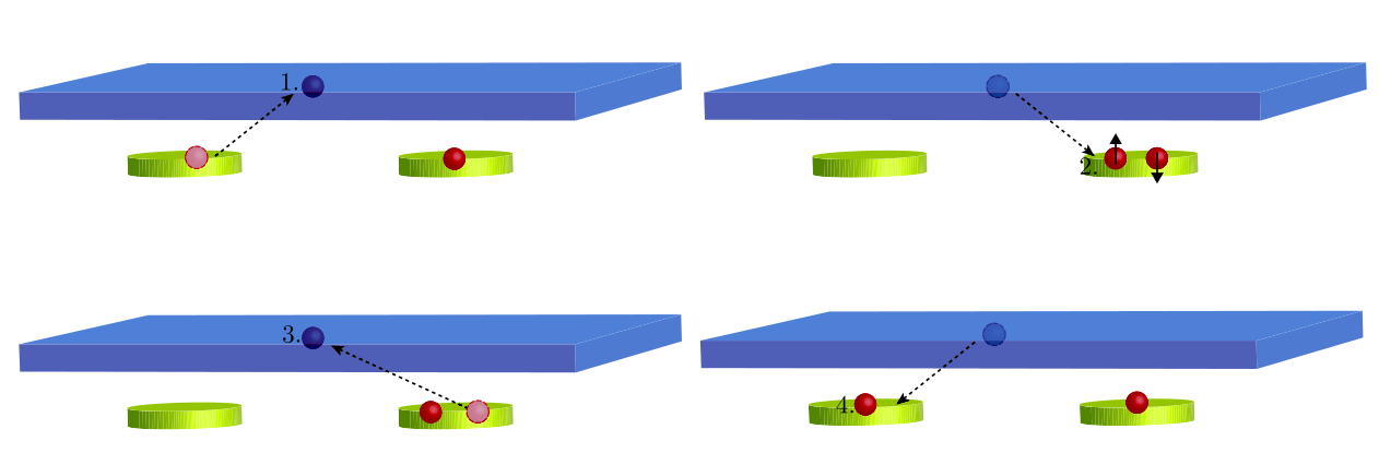
The energies $\varepsilon_{1,1}$ and $\varepsilon_{0,1}$ play a key role in the exchange interaction through the denominator of Eq. (6). Their difference should be minimized in order to increase the effective coupling between the dots. We define the minimum detuning $M$ as the minimum energy difference between the superconducting gap and the energy of an electron in the first dot (see Fig. 2). Due to the broadening of the superconducting density of states, $M$ cannot be arbitrarily low but we can safely assume $M\ll\Delta$. In the absence of a magnetic field, this leads to detuning $\varepsilon_{1,1}-\varepsilon_{0,1}=\epsilon_{1}=\Delta-M$.

The expression for $\alpha$ in Eq. (6) can be written in terms of the electronic Green’s functions in a superconductor. In the two dimensional limit for $M\ll\Delta\ll\mu$, as shown in Ref. Hassler et al. 2015, it assumes the form

with the effective coherence length $\xi_{D}=D^{1/2}/(8\Delta M)^{1/4}$, where $D=v_{F}\ell_{e}/d$ is the diffusion constant and where the electronic Green’s function is defined as

In 2D, the decay of the exchange interactions is controlled by the Macdonald function $K_{0}(x)=\int_{0}^{\infty}\!dt\,\cos[x\sinh(t)]$. Details on how to perform the average over disorder to obtain the result in Eq. (7) can be found in Appendix A.

We want to comment on potential experimental implications of our results. In particular, we would like to estimate the exchange interaction that can be achieved with the setup under discussion. Note that we estimate the strength of the exchange interaction through the dimensionless coupling parameter $\alpha$ [see subsection III.2], which gives the scaling of the exchange interaction in our setup with respect to the microscopic exchange interaction $J_{0}=\Gamma^{2}/\delta\varepsilon$, where we estimate $J_{0}\approx 10-100\,\text{GHz}$. Values of $\alpha$ of the order $10^{-2}-10^{-3}$ are therefore needed to ensure that the exchange interaction remains of the order of $100\,\text{MHz}$, which is a typical value for spin qubit operations Brunner et al. 2011. In order to obtain an improvement in scalability with this setup over current qubit architectures, we aim to achieve such exchange interaction strengths over interdot distances of $R\approx 1\,\mu\text{m}$.

The key elements that determine the strength of the exchange interaction are the effective coherence length in the absence of magnetic field $\xi_{D}$ [defined after Eq. (7)], the geometry of the superconductor, and the strength of the Zeeman splitting. Strictly speaking, the relevant length scale is $\xi_{B}$ and not $\xi_{D}$ [see Eq. (15)]; however, the effect of the Zeeman splitting on the coherence length is weak enough that we can assume $\xi_{B}\approx\xi_{D}$ for order-of-magnitude estimates. The effective coherence length dictates both the decay length of the exchange interaction as well as the dimensionality crossover. At $R\approx\xi_{D}$ the exchange interaction is not yet exponentially suppressed and a superconducting film of width $L_{y}\approx 0.1\xi_{D}$ is sufficient to reach the 1D limit. As we can see in Fig. 4, achieving the 1D limit is a key objective for the optimal use of the setup, since it gives rise to an improvement of more than an order of magnitude over the 2D case. The importance of this improvement is highlighted when an external magnetic field is present, as large exchange interaction under the effect of large Zeeman splittings may only be achievable in the 1D limit (see Fig. 5).

We propose aluminum as a good candidate for the material of the superconducting film. Very thin aluminum films (thickness $L_{x}$ below 10 nm) have a parallel critical field of a few Tesla and their order parameter is not significantly affected by the field up to a substantial fraction of the critical one Catelani et al. 2008. However, the mean free-path $\ell_{e}$ is short, of the order of $L_{x}$. Since the parallel critical field scales as the inverse of the thickness, films of $L_{x}\simeq 30\,$nm should have both sufficiently high critical field (close to 1 T) and sufficiently long mean free-path. Several times longer mean free path can be achieved by epitaxial growth Adams et al. 2017, so we estimate $\ell_{e}\simeq 100\,$nm. With this mean free path, the value of Fermi velocity $v_{F}\simeq 2\times 10^{6}\,$m/s², and the measured spin-orbit scattering rate Catelani et al. 2008; Adams et al. 2017, we arrive at $l_{\text{so}}\sim 1\,\mu$m ³³ 3 We note that this is likely an underestimate of the actual spin-orbit length, since there is evidence that the sheet resistance decreases faster with thickness than one would expect from a linear increase of mean free path with $L_{x}$, and at the same time the spin-orbit scattering time increases with $L_{x}$ Adams et al. 2017; Lo et al. 2015. Since, as discussed in Sec. III.1, $l_{\text{so}}$ sets an upper limit for the effective coherence length $\xi_{D}$, we choose the detuning $M$ so that $\xi_{D}\sim 1\,\mu$m (while neglecting its possible decrease due to finite $l_{\text{so}}$). We therefore set $M=5\times 10^{-3}\Delta\approx 1\,\mu\text{eV}$, where $\Delta\approx 200\,\mu\text{eV}$ is the superconducting gap of aluminum. Such a value for $M$ seems feasible, since the broadening of the peaks in the density of states for aluminum, as measured by the Dynes parameter $\gamma$, can be very small ($\gamma\approx 2\times 10^{-7}\Delta$ Saira et al. 2012). Finally, the prefactor $k_{F}\ell_{e}$ entering $\alpha$, see e.g. Eq. (7), can be rewritten as $2E_{F}\ell_{e}/v_{F}\simeq 2\times 10^{3}$, where $E_{F}=11.6\,$eV is the Fermi energy in aluminum.

The Zeeman splitting depends both on the external magnetic field and the $g$-factors of the materials. For aluminum, a good estimate is $g^{\text{sc}}=2$ at low temperature and for the magnetic fields of interest, since in this case Fermi-liquid effects that renormalize the $g$-factor in the normal state are suppressed Catelani et al. 2008. For the dots, $g^{D}$ can vary depending on several factors, mainly the material hosting the quantum dots and their shape, taking a wide range of values, from negative ones $g^{D}\approx-1$ Belykh et al. 2015; Pryor and Flatté 2006; Shchepetilnikov et al. 2013 to values as large as $g^{D}\approx 50$ Nedniyom et al. 2009, as well as values of the order the free electron one $g^{D}\approx 0.5$–$3$ Katsaros et al. 2010. We assume for simplicity $g^{D}\approx 2$, as appropriate for silicon Ferdous et al. 2018; Zhao et al. 2019, such that external magnetic fields of the order of $B\approx 100\,\text{mT}$ would lead to a total Zeeman splitting $E_{\text{tot}}\approx 10\,\mu\text{eV}\approx 10M$ ⁴⁴ 4 Note that in this case we have $\Delta_{Z}\ll M$ and $M_{B}\simeq M+E_{\text{tot}}$; hence it follows from Eq. (15) that $\xi_{B}/\xi_{D}\approx 0.55$. In the 1D regime for a long strip, this reduces $\alpha$ by a factor of 4, a reduction that can be counteracted by using a finite strip of length $L_{z}\simeq R$.. Looking at Fig. 5, we estimate that using a small enough superconducting strip ($100\,\text{nm}$–$1\,\mu\text{m}$ width) as coupler between two quantum dots an exchange interaction in the order of $J\simeq 100\,\text{MHz}$ over distances of $R\simeq 1\,\mu\text{m}$ can be achieved. This shows that our setup can sustain an external magnetic field up to a few hundred mT and is therefore a viable approach to long-range coupling of spin qubits in a realistic setting.

References

- Arute et al. (2019) F. Arute, K. Arya, R. Babbush, et al., Nature 574, 505 (2019).
- Devoret and Schoelkopf (2013) M. H. Devoret and R. J. Schoelkopf, Science 339, 1169 (2013).
- Bermudez et al. (2017) A. Bermudez, X. Xu, R. Nigmatullin, J. O’Gorman, V. Negnevitsky, P. Schindler, T. Monz, U. G. Poschinger, C. Hempel, J. Home, F. Schmidt-Kaler, M. Biercuk, R. Blatt, S. Benjamin, and M. Müller, Phys. Rev. X 7, 041061 (2017).
- Gaita-Ariño et al. (2019) A. Gaita-Ariño, F. Luis, S. Hill, and E. Coronado, Nat. Chem. 11, 301 (2019).
- Loss and DiVincenzo (1998) D. Loss and D. P. DiVincenzo, Phys. Rev. A 57, 120 (1998).
- Kloeffel and Loss (2013) C. Kloeffel and D. Loss, Annual Review of Condensed Matter Physics 4, 51 (2013).
- Vandersypen et al. (2017) L. M. K. Vandersypen, H. Bluhm, J. S. Clarke, A. S. Dzurak, R. Ishihara, A. Morello, D. J. Reilly, L. R. Schreiber, and M. Veldhorst, npj Quantum Inf. 3, 34 (2017).
- McNeil et al. (2011) R. P. G. McNeil, M. Kataoka, C. J. B. Ford, C. H. W. Barnes, D. Anderson, G. A. C. Jones, I. Farrer, and D. A. Ritchie, Nature 477, 439 (2011).
- Takada et al. (2019) S. Takada, H. Edlbauer, H. V. Lepage, J. Wang, P.-A. Mortemousque, G. Georgiou, C. H. W. Barnes, C. J. B. Ford, M. Yuan, P. V. Santos, X. Waintal, A. Ludwig, A. D. Wieck, M. Urdampilleta, T. Meunier, and C. Bäuerle, Nature Commun. 10, 4557 (2019).
- Baart et al. (2016) T. A. Baart, M. Shafiei, T. Fujita, C. Reichl, W. Wegscheider, and L. M. K. Vandersypen, Nature Nanotech. 11, 330 (2016).
- Nguyen et al. (2017) T. Nguyen, C. D. Hill, L. C. L. Hollenberg, and M. R. James, Sci. Rep. 7, 13386 (2017).
- Wei and Deng (2015) H.-R. Wei and F.-G. Deng, Sci. Rep. 4, 7551 (2015).
- Li et al. (2018) R. Li, L. Petit, D. P. Franke, J. P. Dehollain, J. Helsen, M. Steudtner, N. K. Thomas, Z. R. Yoscovits, K. J. Singh, S. Wehner, L. M. K. Vandersypen, J. S. Clarke, and M. Veldhorst, Science Advances 4 (2018), 10.1126/sciadv.aar3960.
- Busl et al. (2013) M. Busl, G. Granger, L. Gaudreau, R. Sánchez, A. Kam, M. Pioro-Ladrière, S. A. Studenikin, P. Zawadzki, Z. R. Wasilewski, A. S. Sachrajda, and G. Platero, Nature Nanotech. 8, 261 (2013).
- Baart et al. (2017) T. A. Baart, T. Fujita, C. Reichl, W. Wegscheider, and L. M. K. Vandersypen, Nature Nanotech. 12, 26–30 (2017).
- Chan et al. (2020) K. W. Chan, H. Sahasrabudhe, W. Huang, Y. Wang, H. C. Yang, M. Veldhorst, J. C. C. Hwang, F. A. Mohiyaddin, F. E. Hudson, K. M. Itoh, A. Saraiva, A. Morello, A. Laucht, R. Rahman, and A. S. Dzurak, arXiv:2004.07666 (2020).
- Trifunovic et al. (2012) L. Trifunovic, O. Dial, M. Trif, J. R. Wootton, R. Abebe, A. Yacoby, and D. Loss, Phys. Rev. X 2, 011006 (2012).
- Serina et al. (2017) M. Serina, C. Kloeffel, and D. Loss, Phys. Rev. B 95, 245422 (2017).
- Yang et al. (2016) G. Yang, C.-H. Hsu, P. Stano, J. Klinovaja, and D. Loss, Phys. Rev. B 93, 075301 (2016).
- Elman et al. (2017) S. J. Elman, S. D. Bartlett, and A. C. Doherty, Phys. Rev. B 96, 115407 (2017).
- Mi et al. (2017) X. Mi, J. V. Cady, D. M. Zajac, P. W. Deelman, and J. R. Petta, Science 355, 156 (2017).
- Leijnse and Flensberg (2013) M. Leijnse and K. Flensberg, Phys. Rev. Lett. 111, 060501 (2013).
- van Woerkom et al. (2018) D. J. van Woerkom, P. Scarlino, J. H. Ungerer, C. Müller, J. V. Koski, A. J. Landig, C. Reichl, W. Wegscheider, T. Ihn, K. Ensslin, and A. Wallraff, Phys. Rev. X 8, 041018 (2018).
- Scherübl et al. (2019) Z. Scherübl, A. Pályi, and S. Csonka, Beilstein J. Nanotechnol. 10, 363 (2019).
- Hassler et al. (2015) F. Hassler, G. Catelani, and H. Bluhm, Phys. Rev. B. 92, 235401 (2015).
- Wu et al. (2014) X. Wu, D. R. Ward, J. R. Prance, D. Kim, J. K. Gamble, R. T. Mohr, Z. Shi, D. E. Savage, M. G. Lagally, M. Friesen, S. N. Coppersmith, and M. A. Eriksson, Proceedings of the National Academy of Sciences 111, 11938 (2014).
- Takeda et al. (2020) K. Takeda, A. Noiri, J. Yoneda, T. Nakajima, and S. Tarucha, Phys. Rev. Lett. 124, 117701 (2020).
- Shulman et al. (2012) M. D. Shulman, O. E. Dial, S. P. Harvey, H. Bluhm, V. Umansky, and A. Yacoby, Science 336, 202 (2012).
- Fulde (1973) P. Fulde, Advances in Physics 22, 667 (1973).
- Catelani et al. (2008) G. Catelani, X. S. Wu, and P. W. Adams, Phys. Rev. B 78, 104515 (2008).
- Bardeen et al. (1957) J. Bardeen, L. N. Cooper, and J. R. Schrieffer, Phys. Rev. 108, 1175 (1957).
- González Rosado et al. (2020) L. González Rosado, F. Hassler, and G. Catelani, Phys. Rev. B 101, 174202 (2020).
- Danon and Nazarov (2009) J. Danon and Y. V. Nazarov, Phys. Rev. B 80, 041301 (2009).
- Akkermans and Montambaux (2007) E. Akkermans and G. Montambaux, Mesoscopic Physics of Electrons and Photons (Cambridge University Press, 2007).
- (35) We do not include a contribution from , corresponding to cross-terms in the exchange interaction in the form with , as they can be set to zero with a local basis rotation in the -plane.
- (36) If the -factors have different sign, or if SO coupling is weak (such that the possible decay into the superconductor due to spin non-conserving tunneling as electrons reach energies higher than could be neglected), the energy tuning would give stronger exchange interaction.
- Gawełczyk and Gawarecki (2019) M. Gawełczyk and K. Gawarecki, arXiv:1902.10112 (2019).
- Danon (2013) J. Danon, Phys. Rev. B 88, 075306 (2013).
- Maisi et al. (2016) V. F. Maisi, A. Hofmann, M. Röösli, J. Basset, C. Reichl, W. Wegscheider, T. Ihn, and K. Ensslin, Phys. Rev. Lett. 116, 136803 (2016).
- Brunner et al. (2011) R. Brunner, Y.-S. Shin, T. Obata, M. Pioro-Ladrière, T. Kubo, K. Yoshida, T. Taniyama, Y. Tokura, and S. Tarucha, Phys. Rev. Lett. 107, 146801 (2011).
- Adams et al. (2017) P. Adams, H. Nam, C. K. Shih, and G. Catelani, Phys. Rev. B 95, 094520 (2017).
- (42) We note that this is likely an underestimate of the actual spin-orbit length, since there is evidence that the sheet resistance decreases faster with thickness than one would expect from a linear increase of mean free path with , and at the same time the spin-orbit scattering time increases with Adams et al. 2017; Lo et al. 2015.
- Saira et al. (2012) O.-P. Saira, A. Kemppinen, V. F. Maisi, and J. P. Pekola, Phys. Rev. B 85, 012504 (2012).
- Belykh et al. (2015) V. V. Belykh, A. Greilich, D. R. Yakovlev, M. Yacob, J. P. Reithmaier, M. Benyoucef, and M. Bayer, Phys. Rev. B 92, 165307 (2015).
- Pryor and Flatté (2006) C. E. Pryor and M. E. Flatté, Phys. Rev. Lett. 96, 026804 (2006).
- Shchepetilnikov et al. (2013) A. V. Shchepetilnikov, Y. A. Nefyodov, I. V. Kukushkin, and W. Dietsche, Journal of Physics: Conference Series 456, 012035 (2013).
- Nedniyom et al. (2009) B. Nedniyom, R. J. Nicholas, M. T. Emeny, L. Buckle, A. M. Gilbertson, P. D. Buckle, and T. Ashley, Phys. Rev. B 80, 125328 (2009).
- Katsaros et al. (2010) G. Katsaros, P. Spathis, M. Stoffel, F. Fournel, M. Mongillo, V. Bouchiat, F. Lefloch, A. Rastelli, O. G. Schmidt, and S. D. Franceschi, Nature Nanotech. 5, 458–464 (2010).
- Ferdous et al. (2018) R. Ferdous, E. Kawakami, P. Scarlino, M. P. Nowak, D. R. Ward, D. E. Savage, M. G. Lagally, S. N. Coppersmith, M. Friesen, M. A. Eriksson, L. M. K. Vandersypen, and R. Rahman, npj Quantum Inf. 4, 26 (2018).
- Zhao et al. (2019) T. Zhao, R.and Tanttu, K. Y. Tan, B. Hensen, K. W. Chan, J. C. C. Hwang, R. C. C. Leon, C. H. Yang, W. Gilbert, F. E. Hudson, K. M. Itoh, A. A. Kiselev, T. D. Ladd, A. Morello, A. Laucht, and A. S. Dzurak, Nature Commun. 10, 5500 (2019).
- (51) Note that in this case we have and ; hence it follows from Eq. (15) that . In the 1D regime for a long strip, this reduces by a factor of 4, a reduction that can be counteracted by using a finite strip of length .
- Abrikosov et al. (1975) A. Abrikosov, L. Gorkov, and I. Dzyaloshinski., Methods of Quantum Field Theory in Statistical Physics (Dover Publications, INC., 1975).
- Bravyi et al. (2011) S. Bravyi, D. P. DiVincenzo, and D. Loss, Annals of Physics 326, 2793 (2011).
- Lo et al. (2015) S.-T. Lo, S.-W. Lin, Y.-T. Wang, S.-D. Lin, and C.-T. Liang, Sci. Rep. 4, 5438 (2015).