Revisiting Factorizing Aggregated Posterior
in Learning Disentangled Representations
Abstract
In the problem of learning disentangled representations, one of the promising methods is to factorize aggregated posterior by penalizing the total correlation of sampled latent variables. However, this well-motivated strategy has a blind spot: there is a disparity between the sampled latent representation and its corresponding mean representation. In this paper, we provide a theoretical explanation that low total correlation of sampled representation cannot guarantee low total correlation of the mean representation. Indeed, we prove that for the multivariate normal distributions, the mean representation with arbitrarily high total correlation can have a corresponding sampled representation with bounded total correlation. We also propose a method to eliminate the above-mentioned disparity. Experiments show that our model can learn a mean representation with much lower total correlation, hence a factorized mean representation. Moreover, we offer a detailed explanation of the limitations of factorizing aggregated posterior: factor disintegration. Our work indicates a potential direction for future research of disentangled learning.
Keywords:
Total Correlation, Representative Learning, DisentanglementDisentangled representation is believed to be the key to learn a better representation (Bengio et al., 2013; LeCun et al., 2015; Peters et al., 2017). There are 2 major ingredients of disentanglement: 1. Models should learn separate factors of variations (Bengio et al., 2013); 2. Factors should be compact (Bengio et al., 2013), informative and independent from task at hand (Goodfellow et al., 2009). The motivation of disentanglement includes usefulness for downstream tasks (Bengio et al., 2013), being invariant to nuisance factors (Kumar et al., 2017), improving robustness to adversarial attack (Alemi et al., 2016), etc. (See also the introduction of disentangled representation in Locatello et al., 2018; Chen et al., 2018; Kim and Mnih, 2018 and reference therein.)
Recent works (Higgins et al., 2017; Kim and Mnih, 2018; Chen et al., 2018; Kumar et al., 2017; Ridgeway and Mozer, 2018) have introduced various regularizers to the objective function of the Variational Autoencoder (VAE) (Kingma and Welling, 2013; Bengio et al., 2007), Evidence Lower Bound (ELBO). They aim at factorizing aggregated posterior, , which hopefully can encourage disentanglement. Among these works, Kim and Mnih, 2018; Chen et al., 2018 independently proposed a promising regularizer, the total correlation (TC) of sampled representation. TC is defined to be the KL-divergence between the joint distribution and the product of marginal distributions . The TC of a sampled representation, , should describe its level of independence. In this case, a low value suggests a more factorized joint distribution.
However, Locatello et al., 2018 point out, though these works seem to be effective at factorizing aggregated posterior, there exists a blind spot: a disparity between and the TC of the corresponding mean representation, . Specifically, A low does not necessarily give rise to a low . Conventionally, the mean representation is used as the encoded latent variables, an unnoticed high is usually the culprit behind the undesirable entanglement. They found that as the strength of regularization on increases, decreases as expected, but increases. Moreover, the scores under disentanglement metrics are uncorrelated to the regularization strength. Their finding has 2 implications:
- 1.
Low does not imply low , which is yet not understood;
- 2.
Either low or low does not guarantee disentanglement. Disentanglement does not seem to correlate with or no matter how much these 2 quantities change.
This created several important yet not answered questions: Why does have no control over ? Is the strategy of regularizing TC unhelpful to disentanglement? In this paper, we answer the first question completely by theoretically analyzing the relation between and . Then after investigating factorized representations, we believe that regularizing TC still might be a key to learning disentangled representation and hopefully our study can shed some light into this problem.
Our main contributions are listed as the followings:
- •
- •
We show how to control both and and obtain factorized mean representation. Our method is to introduce a simple yet effective regularizer, a penalty term on the variance of each latent variable, which forces a sampled representation to behave similarly to the corresponding mean representation. (Section. 3)
- •
We compare different methods of TC estimation and point out that the method of minibatch estimators (MSS/MWS) suffers from the curse of dimensionality, i.e., the estimation accuracy decays significantly with the increase of the dimension of the latent space. In addition, they may cause unintended shutdown of latent dimensions. (Section. 4)
- •
We investigate the limitation of factorized mean representation and suggest a tradeoff be considered for the future work of learning disentangled representation. (Section. 5)
1 Related Works
VAE (Kingma and Welling, 2013; Bengio et al., 2007) takes the variational approach to approximate the posterior with by minimizing their KL-divergence, , which is equivalent to maximizing ELBO. As a result, the high-dimensional real world observations is encoded into lower-dimension latent variable that is expected to be semantically meaningful.
In order to learn disentangled representation, Higgins et al., 2017 proposed a modification of the VAE framework and introduced an adjustable hyperparameter that balances latent channel capacity and independence constraints with reconstruction accuracy.
Chen et al., 2018 proposed -TCVAE which adopts the idea of decomposing the average ELBO (Hoffman and Johnson, 2016) and penalizes the TC of latent variables aiming on regularizing a more precise source of disentanglemnet. Around the same time, Kim and Mnih, 2018 proposed a similar regularizer penalizing called FactorVAE. The major difference between FactorVAE and -TCVAE lies in their different strategies of estimating . Chen et al., 2018 used formulated estimators while Kim and Mnih, 2018 utilized the density-ratio trick which requires an auxiliary discriminator network. We will discuss these two strategies more in details in Section. 4. Kumar et al., 2017 introduced DIP-VAE-I&II, which penalize on the covariance matrix of mean and sampled latent variables respectively in order to encourage disentanglement. This strategy could learn an uncorrelated but not independent distribution.
Locatello et al., 2018 challenged most recent work on disentanglement and argued that unsupervised learning of disentangled representations without inductive biases is basically impossible. This makes strong suggestion that researchers should pay attention to representative learning with inductive biases on both learning approaches and data sets. We refer readers to works in this direction, e.g. Thomas et al., 2018; Bouchacourt et al., 2018; Rolinek et al., 2019 and works referred therein. However, Locatello et al., 2018 does not provide an explanation to one of the observations they made, i.e., why most regularizers are effective at factorizing aggregated posterior but the corresponding mean representations may be entangled? We answer this question in the next section.
2 The Disparity between Total Correlation of Mean and Sampled Distribution
In information theory, total correlation (TC) is one of the generalizations of mutual information (see definition 1), which measures the difference between the joint distribution of multiple random variables and the product of their marginal distributions. A high value of TC indicates the joint distribution is far from an independent distribution, and hence it suggests high entanglement among these random variables.
Definition 1.
The total correlation of random variable is defined as
Motivated by this concept, people seek the solution of disentanglement in the form of low TC of the latent variables (Kim and Mnih, 2018; Chen et al., 2018). However, Locatello et al., 2018 pointed out that even though is low, can be high. This is problematic because the mean representation is usually taken as the representation of input and such representation is entangled.
Hence, a clear understanding of the relation between and is needed. To this end, we present a theorem that provides an explicit bound for under some mild assumptions. This bound does not rely on the distribution of mean representation, which turns out to be the root of the disparity between the two TCs. One of the assumptions we made is that the distribution of mean representation is multivariate normal (MVN), but actually the theorem can be easily generalized to distributions with compact support or fast decay. This makes the theorem relatively general and effective for many practical cases.
Here are some notations: and are random variables, and and are corresponding samples (fixed values); and are matrices; stands for some constant.
Theorem 1.
Let . For a fixed , let , where is diagonal and satisfies that,
| (1) |
where and is the diagonal element of . Then is independent of and
| (2) |
where and is some constant that replies only on dimension .
The details of the proof are presented in Appendix 2. Intuitively, in the case of multivariate normal distribution, if there exist two dimensions of with high correlation, then the TC of this distribution is high (less independent). And the probability density is narrowly distributed in the subspace of these two dimensions. Now, if the standard deviations of corresponding to these two dimensions are suitably large (bounded away from zero), then the distribution of will spread wider in the subspace which is closer to a distribution with low TC (more independent). Figure 1 gives an example, for a distribution of with high TC, how to construct distribution of with low TC.
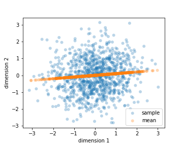
One fact can be deduced from Theorem 1 is: with a fixed upperbound of (by fixing parameters ), one can make arbitrarily large. To see this, we use Proposition 1 in Section. 4, which states depends only on the determinant of the correlation matrix of , i.e., , so we only need to tune the off-diagonal elements of (while keeping unchanged) to make go to zero and hence go to infinity.
Interestingly, we note that in Theorem 1 when approaches zero, the upperbound of goes to infinity. It reflects the following fact: when the distribution of is closed to the distribution of , is close to , which can be large.
Thus, Theorem 1 provides an explanation to the disparity observed by Locatello et al., 2018 that is low but is high. Indeed, for every distribution of with large there exist a family of distributions of with bounded . If the objective function only penalizes , the optimization process could easily find a distribution of with low but high . However, this disparity can be eliminated. In Section. 3, we propose a simple regularizer to serve this goal.
3 An Additional Regularizer
To simplify notation, let , and . Recall the average evidence lower bound (ELBO):
| (3) |
where the first term can be interpreted as reconstruction error. Inspired by ELBO decomposition (Hoffman and Johnson, 2016), Chen et al., 2018 refined the decomposition and separated TC of from other terms. Since the independence of latent variables can be one of the sources of disentanglement, they introduced -TCVAE with a new objective function that penalizes TC in order to learn factorized representation. At the same time, also recognizing the importance of TC in factorizing aggregated posterior, Kim and Mnih, 2018 independently introduced FactorVAE that penalizes with a different implementation. Such strategy of penalizing can be formulated as
| (4) |
Though this strategy are effective at factorizing aggregated posterior (Locatello et al., 2018), according to Theorem 1 the mean representations can still be entangled. To resolve this, we propose a regularized TC-VAE (RTC-VAE),
| (5) |
where Our penalty originates from the first term of the law of total covariance:
Note that a factorized distribution must have a diagonal covariance matrix . For VAEs, it is conventional to set as a factorized distribution, e.g. , which forces VAEs to behave similar to PCA (Rolinek et al., 2019). As a result, the first term is forced to be diagonal.
Motivated by this, Kumar et al., 2017 proposed DIP-VAEs which penalizes the off-diagonal terms in the second term in the law of total correlation and ignores the first term in order to get a diagonal covariance matrix . Locatello et al., 2018 recognized DIP-VAEs being effective on factorizing aggregated posterior, but we point out that this is actually mistaken. The reason is simply because zero correlation does not necessarily imply independence (see details in Section 5).
Our approach, on the other hand, does not penalize directly on . Instead, we penalize on , the standard deviation of the distribution , which is the first term in the law of total covariance. This may seem little counter-intuitive at first sight, since penalizing a diagonal component of covariance seems not helpful to factorising. However, in the view of Theorem 1, the additional regularizer in equation 5 will force the distribution of to be similar to the distribution of . Hence, it pushes us away from the situation of large and low . Consequently, by minimizing we get low , which leads to factorized mean representations.
In practice, we keep in a range, e.g., , by multiplying the hyperparameter with 1.2 if this term is greater than and set to zero if the term is smaller than . If the variance of latent variables vanishes completely, the VAE degenerates to a deterministic autoencoder. Thus, this approach saves the effort of tuning extra hyperparameter and keeps the stochastic nature of VAE.
4 Estimation of Total Correlation

To calculate the objective function equation 5, a key step is to estimate TC. For multivariate normal distribution11 1 One may choose other prior distributions for a VAE model for different reasons. Here, normal distribution helps our analysis and simplifies the scenario. This is the reason why we choose normal distribution as prior. , its ground truth TC can be explicitly calculated thanks to the following proposition,
Proposition 1.
Let , then
| (6) |
Proposition 1 is a simple result, which is why its exact originality is difficult to track, but it is quite handy in our analysis. In Appendix 3, we provide a simple proof for the convenience of readers. Locatello et al., 2018 even used this proposition to approximate the TC of the mean representations in latent space.
To estimate TC, naive Monte Carlo method comes with an intrinsic issue of underestimation. To resolve this, Kim and Mnih, 2018 proposed a discriminator network with the help of density-ratio trick (see equation (3) and Appendix D. of Kim and Mnih, 2018). In Chen et al., 2018, two kinds of estimator of TC are proposed, Minibatch Weighted Sampling (MWS) and Minibatch Stratified Sampling (MSS) (see definitions in Appendix 1).
In this work, we adopt density-ratio trick as our main method for estimating the total correlation of RTC-VAE. The reason is that we found out there exist some problems of MWS and MSS: the curse of dimensionality and an unintended latent dimension shutdown.
Our anaysis on MWS and MSS consists of both experimental and theoretic analysis. First, we evaluate MWS, MSS0 and MSS1 (see definitions in Appendix 1) through the following experiments. Let where , and where and . We set small so that the distribution of can be approximated by normal distribution, and the ground truth can be calculated by Proposition 1. Then by adjusting , we can control . We evaluate different estimators on different TC’s, and results are presented in Figure 2.
From the experiments, we summarize some observations: 1. MWS tends to underestimate TC in general; 2. For latent space of dimension , MSS0 and MSS1 are relatively accurate; 3. For latent space of high dimension, both MSS0 and MSS1 tend to overestimate TC when the actual value of TC is small; 4. Overall MSS1 estimates closer to ground truth than MMS0 does.
In Appendix 1, we provides a theoretic analysis of the 3rd observation to explain why these estimators deteriorate as dimension increases. In addition, we find that MWS and MSS may lead to an unintended shutdown of latent dimensions. While shutting down dimensions may not necessarily hurt disentanglement (it even can be helpful), the shutdown caused by these estimators is yet less understood for practice. We refer readers to Appendix 1 for detailed analysis.
Density-ratio trick and auxiliary discriminator: The gist of density-ratio trick is to estimate the KL-divergence between the distribution of the latent representation and the distribution of factorized latent representations , which can be described as following (Nguyen et al., 2010; Sugiyama et al., 2012),
| (7) |
where is discriminator that classifies being sampled from or . We implemented our TC estimator according to Section 3 in Kim and Mnih, 2018 for training the auxiliary network .
We do not include a direct numerical comparison between density-ratio trick and MWS/MSS because density-ratio trick would gain unfair advantage due to a potentially overfitting auxiliary discriminator.
5 Experiments
We compare RTC-VAE with three models: FactorVAE and DIP-VAE-I&II. We saved the experiments on -TCVAE because its problem of disparity is the same as FactorVAE (Locatello et al., 2018). The datasets we use include dSprites (Matthey et al., 2017), Shapes3D (Burgess and Kim, 2018) and Car3d (Reed et al., 2015). Check Table 2 for the architectures of encoder and decoder and Table 1 for hyper-parameter setting. More details of experiments can be found in Appendix 7. We use the same structure for discriminator as Kim and Mnih, 2018 suggested for FactorVAE, which is a 6-layer MLP with 1000 hidden units per layer and leaky ReLU activation.
For RTC-VAE, we set the hyperparameter . We bound from below to avoid the situation where the variance term in equation 5 is so small that it will not contribute much compared with the term. Especially when is small, we need strong enough to regularize .
We choose batch size 500 for all models on all data sets to balance between performance and training time, whereas Locatello et al., 2018; Kim and Mnih, 2018 used 64, Kumar et al., 2017 used 400 and Chen et al., 2018 used 2048 to account for the bias in minibatch estimation. Learning rate is fixed to . We evaluate models on 5000 randomly sampled data on every data set.
We estimate and by Proposition 1 as proposed by Locatello et al., 2018. Specifically, we calculate the correlation matrices of the mean and sampled latent vectors, ’s and ’s, encoded from the 5000 samples.
5.1 Eliminating the Disparity between and
We first show that RTC-VAE has eliminates the disparity between and . Again, since -TCVAE has the same problem of disparity as FactorVAE, it is sufficient to compare RTC-VAE with FactorVAE. In order to do that, we evaluate and of RTC-VAE under different regularization strength and compare them with the corresponding values of FactorVAE.
In Figure 3, we see that: (Left) Under all regularization strength, the disparity exists between and for both -VAE and FactorVAE. (Right) With the regularizer on variance of , there is almost no difference between and , i.e., the disparity is evidently remedied. In Figure 4, the revised -VAE and FactorVAE can obtain much lower and than vanilla ones, meanwhile their are comparably low.


5.2 Factorizing Aggregated Posterior
Locatello et al., 2018 reported that DIP-VAEs seem to be immune to the disparity between TCs and pointed out it is due to the measurement of TC being Gaussian based. Since DIP-VAEs are trained by regularizing the off-diagonal elements of correlation matrix, by Proposition 1 they are guaranteed to have low estimated TCs. Then the question is: Do DIP-VAEs obtain really factorized representation? Our investigation shows that the answer is no.
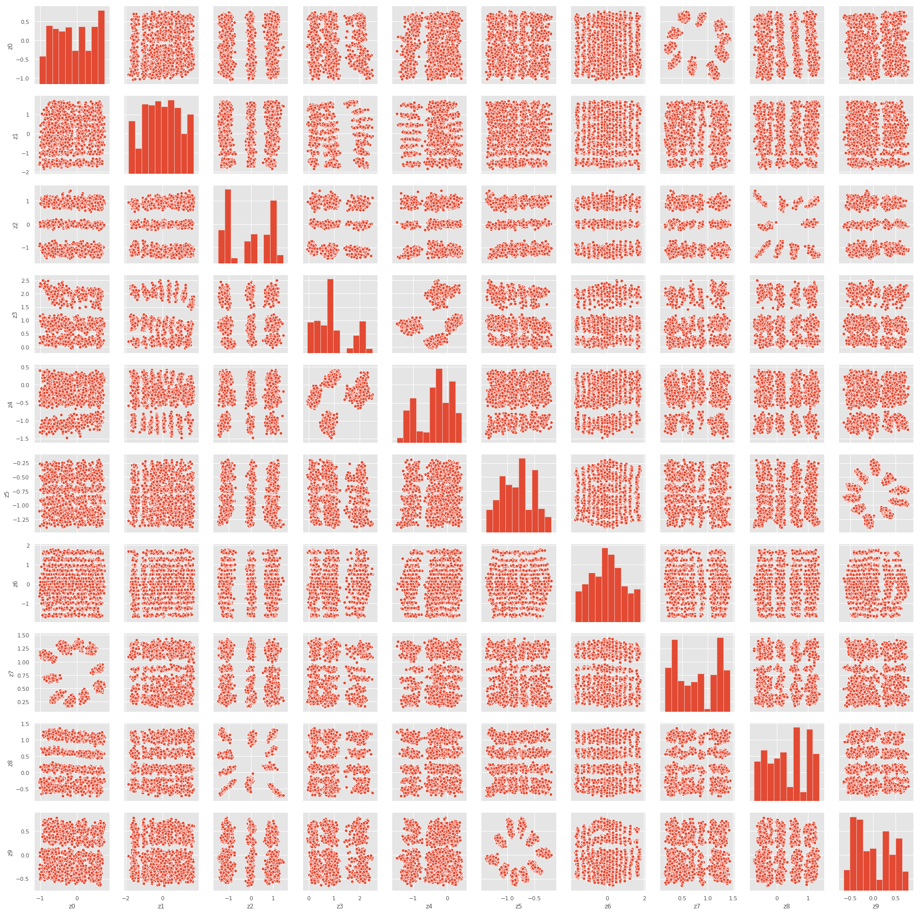
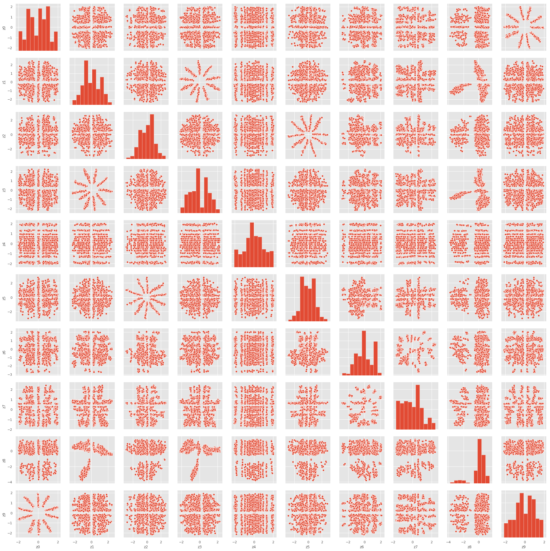
In Figure 5 (c) and also Figure 6, we see that the learned latent representations of DIP-VAEs are uncorrelated but not factorized. Notice that estimating TC by Proposition 1 is only valid for the multivariate normal distribution. If the presumption is violated, any uncorrelated distribution will have zero TC by such estimation. Since DIP-VAEs penalize directly on the correlation of mean representations, it leads to uncorrelated distributions and low TC estimation. Yet an uncorrelated and non-Gaussian distribution is not necessarily independent or factorized.


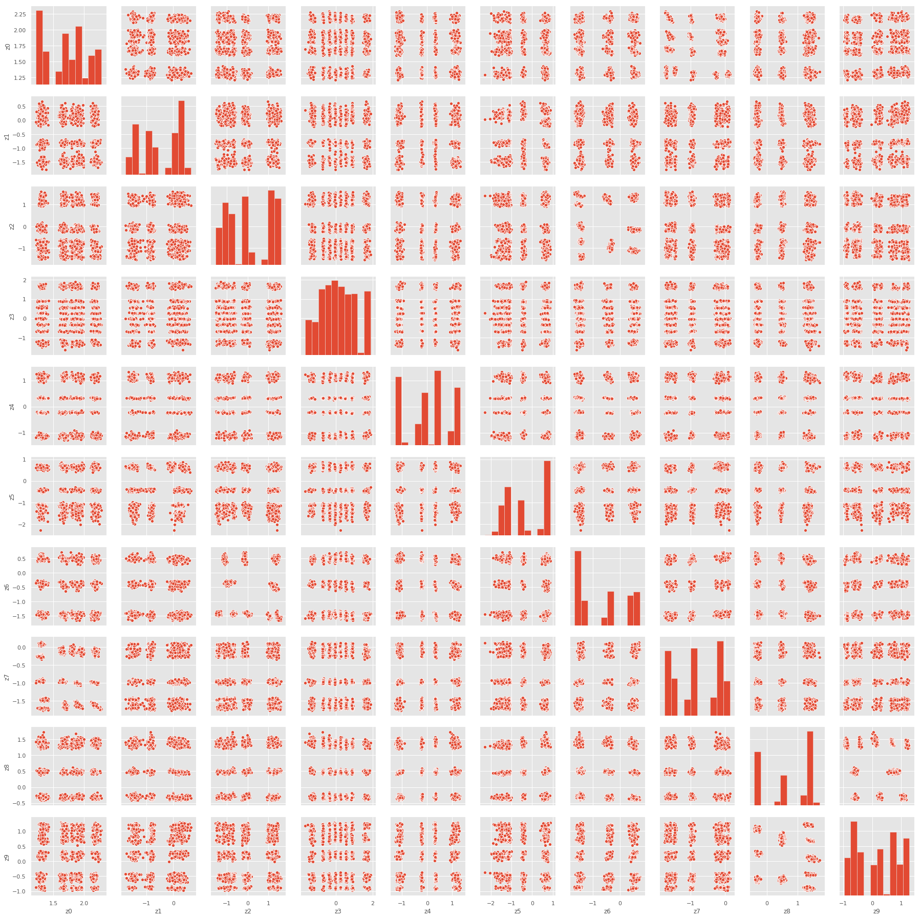
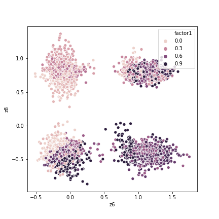
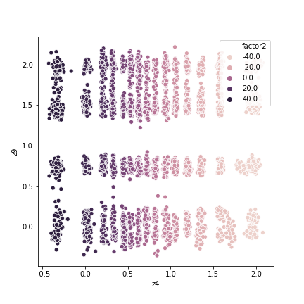
On the other hand, RTC-VAE can successfully factorize representations (both sample and mean). Since the mean and sampled representation are very close, we only need to examine one of them. A typical distribution of latent variables learned by RTC-VAE is presented in the pairplot of all latent variables, see Figure 5 (d) and also Figure 15 in Appendix 7. We observe that the distribution present features of discrete independent distributions.
5.3 Factor Disintegration: Is Factorized Representation Disentangled?
Now that we can obtain factorized representations, the next question is: is a factorized representation disentangled? Here, we point out factor disintegration, indicating multiple independent latent variables simultaneously represent one single factor of variation, exists in factorized representation, which maybe an unwanted feature for disentanglement. To this end, future study of disentangled representation should consider this tradeoff between factor disintegration and factorized representations.
First, we will describe what factor disintegration is. For example, in Shape3D, the wall hue is a 1-d factor taking values between 0 and 1. It turns out that a VAE model can cause the 1-d factor to disintegrate into 2 or more latent variables. Then each latent variable controls a subset of wall hue. In this way, even though the VAE can have a highly factorized latent representation, it manages to use multiple dimensions to represent the wall hue instead of one, hence a factor disintegration (see Figure 5 (b) and (d)).
Factor disintegration disobeys the notion of “compactness” introduced by Eastwood and Williams, 2018, where compactness indicates each factor associates only one or a few latent variables. So, factor disintegration is a subclass of non-compactness (additionally presuming independence). Though there is still disagreement on whether compactness should be a character of disentanglement, e.g., Ridgeway and Mozer, 2018, factor disintegration can potentially lead to unnecessarily many latent variables associating to a single factor of variation.


5.4 The Effect of Factor Disintegration on Disentanglement Metric
To further demonstrate how factor disintegration will affect disentangled learning, we analyze its effect on disentanglement metric.
There are many disentanglement metrics, and most of these metrics share something in common. They look for the link between each factor of variation and each latent variable though the way of measuring the link differs. For example, Chen et al., 2018 proposed mutual information gap (MIG), which estimates the mutual information between each latent variable and each ground truth factor and then find the average gap between top 2 scores. DCI (Eastwood and Williams, 2018) computes the uncertainty (entropy) of predicting ground truth factor by latent variables, and then constructs a weighted average as a score. Higgins et al., 2017 proposed BetaVAE, a linear classifier that predicts the index of a fixed factor of variation. Then they use the accuracy of the classifier as a disentanglement metric. Kim and Mnih, 2018 improved this method by using majority vote classifier to handle some corner case.
As Locatello et al., 2018 pointed out, most metrics could actually be mildly correlated, and pairs (BetaVAE, FactorVAE) and (MIG, DCI) are even strongly correlated with each other. It implies that no matter which metric we use, if a model is affected by factor disintegration, it can find multiple latent variables scoring similar values, and hence suppress its final score under such metric.
In the following, we test the argument above with two disentanglement metrics: MIG and Separated Attribute Predictability score (SAP score), proposed by Kumar et al., 2017 . Both metrics are classifier-free and essentially independent of the data. The idea behind SAP is similar to MIG but the underline measurement is score instead of mutual information. Specifically, SAP computes score between each latent variable and ground truth factor, and then calculate the difference between top 2 scores for each ground truth factor, and lastly take the average of these differences as a final score. Considering the theoretically optimal case (i.e., every ground truth factor is linearly correlated with exactly one latent variable and uncorrelated with all other variables), SAP score has an optimal value 1 (see evaluation of models with SAP in Appendix 7), whereas MIG is bounded above by the average entropy of each ground truth factor.
6 Conclusion
In this work, we theoretically explain the relation between TC of sampled and mean distribution. We analyze the methods of estimating TC and point out some unnoticed problem. We demonstrate that RTC-VAE can eliminates the disparity between TC of the sampled and mean representations. Also, we compare RTC-VAE with DIP-VAEs and point out that DIP-VAEs can end up with uncorrelated yet dependent latent variables. Last, we find out a tradeoff between factorizing aggregated posterior and factor disintegration underlines disentangling representation.
References
- Alemi et al., (2016) Alemi, A. A., Fischer, I., Dillon, J. V., and Murphy, K. (2016). Deep variational information bottleneck. arXiv preprint arXiv:1612.00410.
- Bengio et al., (2013) Bengio, Y., Courville, A., and Vincent, P. (2013). Representation learning: A review and new perspectives. IEEE transactions on pattern analysis and machine intelligence, 35(8):1798–1828.
- Bengio et al., (2007) Bengio, Y., LeCun, Y., et al. (2007). Scaling learning algorithms towards ai. Large-scale kernel machines, 34(5):1–41.
- Bouchacourt et al., (2018) Bouchacourt, D., Tomioka, R., and Nowozin, S. (2018). Multi-level variational autoencoder: Learning disentangled representations from grouped observations. In Thirty-Second AAAI Conference on Artificial Intelligence.
- Burgess and Kim, (2018) Burgess, C. and Kim, H. (2018). 3d shapes dataset. https://github.com/deepmind/3dshapes-dataset/.
- Chen et al., (2018) Chen, R. T., Li, X., Grosse, R., and Duvenaud, D. (2018). Isolating sources of disentanglement in vaes. arXiv preprint arXiv:1802.04942.
- Eastwood and Williams, (2018) Eastwood, C. and Williams, C. K. (2018). A framework for the quantitative evaluation of disentangled representations.
- Goodfellow et al., (2009) Goodfellow, I., Lee, H., Le, Q. V., Saxe, A., and Ng, A. Y. (2009). Measuring invariances in deep networks. In Advances in neural information processing systems, pages 646–654.
- Higgins et al., (2017) Higgins, I., Matthey, L., Pal, A., Burgess, C., Glorot, X., Botvinick, M., Mohamed, S., and Lerchner, A. (2017). beta-vae: Learning basic visual concepts with a constrained variational framework. ICLR, 2(5):6.
- Hoffman and Johnson, (2016) Hoffman, M. D. and Johnson, M. J. (2016). Elbo surgery: yet another way to carve up the variational evidence lower bound.
- Kim and Mnih, (2018) Kim, H. and Mnih, A. (2018). Disentangling by factorising. arXiv preprint arXiv:1802.05983.
- Kingma and Welling, (2013) Kingma, D. P. and Welling, M. (2013). Auto-encoding variational bayes. arXiv preprint arXiv:1312.6114.
- Kumar et al., (2017) Kumar, A., Sattigeri, P., and Balakrishnan, A. (2017). Variational inference of disentangled latent concepts from unlabeled observations. arXiv preprint arXiv:1711.00848.
- LeCun et al., (2015) LeCun, Y., Bengio, Y., and Hinton, G. (2015). Deep learning. nature, 521(7553):436–444.
- Locatello et al., (2018) Locatello, F., Bauer, S., Lucic, M., Gelly, S., Schölkopf, B., and Bachem, O. (2018). Challenging common assumptions in the unsupervised learning of disentangled representations. arXiv preprint arXiv:1811.12359.
- Matthey et al., (2017) Matthey, L., Higgins, I., Hassabis, D., and Lerchner, A. (2017). dsprites: Disentanglement testing sprites dataset. https://github.com/deepmind/dsprites-dataset/.
- Nguyen et al., (2010) Nguyen, X., Wainwright, M. J., and Jordan, M. I. (2010). Estimating divergence functionals and the likelihood ratio by convex risk minimization. IEEE Transactions on Information Theory, 56(11):5847–5861.
- Peters et al., (2017) Peters, J., Janzing, D., and Schölkopf, B. (2017). Elements of causal inference: foundations and learning algorithms. MIT press.
- Reed et al., (2015) Reed, S. E., Zhang, Y., Zhang, Y., and Lee, H. (2015). Deep visual analogy-making. In Advances in neural information processing systems, pages 1252–1260.
- Ridgeway and Mozer, (2018) Ridgeway, K. and Mozer, M. C. (2018). Learning deep disentangled embeddings with the f-statistic loss. In Advances in Neural Information Processing Systems, pages 185–194.
- Rolinek et al., (2019) Rolinek, M., Zietlow, D., and Martius, G. (2019). Variational autoencoders pursue pca directions (by accident). In Proceedings of the IEEE Conference on Computer Vision and Pattern Recognition, pages 12406–12415.
- Sugiyama et al., (2012) Sugiyama, M., Suzuki, T., and Kanamori, T. (2012). Density-ratio matching under the bregman divergence: a unified framework of density-ratio estimation. Annals of the Institute of Statistical Mathematics, 64(5):1009–1044.
- Thomas et al., (2018) Thomas, V., Bengio, E., Fedus, W., Pondard, J., Beaudoin, P., Larochelle, H., Pineau, J., Precup, D., and Bengio, Y. (2018). Disentangling the independently controllable factors of variation by interacting with the world. arXiv preprint arXiv:1802.09484.
Appendix
1 Problems in Methods of Minibatch Estimators
1.1 Minibatch Weighted Sampling (MWS)
See Chen et al., 2018,
| (8) |
1.2 Minibatch Estimators (MSS)
MSS can be described as: For a minibatch of sample, ,
| (9) |
where
| (10) | ||||
| (11) |
is an unbiased estimator of , but it turns out when it is used for estimating TC, it suffers from the curse of dimensions.
MMS0 and MMS1: There is a small part of the implementation of MSS in Chen et al.’s code that is not quite clear to us, specifically, the computation of log importance weight matrix in equation 9. In our experiment, we implement MSS with our understanding and denote it as MSS1, and we denote Chen et al.’s implementation MSS0. The only difference is that we replace this chunk of code (https://github.com/rtqichen/beta-tcvae/blob/master/vae_quant.py#L199-L201) to
1.3 Comparison of the Two Methods
In Section 4 we present our empirical evaluation of MWS, MSS0 and MSS1, and the result is shown in Figure 2. Here, we conduct some theoretical analysis and try to explain some of our observations: For latent space of dimension , MSS0 and MSS1 are relatively accurate; for latent space of high dimension, both MSS0 and MSS1 tend to overestimate TC when the actual value of TC is small.
Recall the experiment settings: Let where , and where and . We set small so that the distribution of can be approximated by normal distribution, and the ground truth can be calculated by Proposition 1. Then by adjusting , we can control .
1.3.1 The Curse of Dimensionality
Let be the batchsize and be the dimensions of latent space. Notice that in the above setting and is small. Let be the estimation of with minibatch estimator, either equation 9 or equation 8, and we find that for approximately
| (12) |
See details of deduction in Appendix 5. Thus, seriously overestimates the true .
1.3.2 Unintended Shutdown of Latent Dimensions
We also find that the estimation of TC by MSS and MWS is lower for distributions with few active latent dimensions (we refer it as dimension “shutdown”) than distributions with fully active dimensions. To see why, consider , where , and where means all the dimensions except 0, and assume that is uncorrelated with the rest, and , where . Again, and if we choose small , is small.
Though a similar analysis we find that the estimation of is approximately
| (13) |
See a proof in Appendix 6. Compared to equation 12, the distribution with a shutdown dimension has a lower estimation of TC. Hence, by penalizing estimated a model may converge to distribution with fewer active latent variables.
We note that shutting down latent dimensions may be helpful to learning disentangled representation, e.g., if the number of ground truth dimensions can efficiently represent data, more dimensions may cause entanglement. There are some works studying the phenomenon of dimension shutdown of VAE, and readers may refer to Rolinek et al., 2019 and reference therein. However, in the case of MWS/MSS, the shutdown may be unintended and it is yet unclear exactly how many dimensions get shutdown. In our opinion, in order to precisely induce dimension shutdown, a better solution may be introducing proper bias to models, which also motivates supervised learning to disentangled learning (in addition to regularizing factor disintegration discussed in Section 5.3).
2 Proof of Theorem 1
In the following proof, we follow a convention of mathematical analysis: the meaning of can change through lines. Specifically, if there are and , take . Since we only care about boundedness of some quantity, this notation eliminates some redundant work of tracking. .
Theorem (Theorem 1 restated).
Let . For a fixed , let , where is diagonal and satisfies that,
| (14) |
where and is the diagonal element of . Then is independent of and
| (15) |
where and is some constant that replies only on dimension .
Proof. Let
then
Since KL-divergence is non-negative, if is bounded, then must be bounded. In the following, we work on , i.e., we assume .
Note that total correlation is invariant under scaling, i.e., for , , then . In Gaussian case, one can see this by simply applying Proposition 1. Hence, let be the standard deviation of , and we can assume . Otherwise we can instead work on with a sufficient small .
Fix some , and for ,
And also for ,
where in the second last inequality we use the fact and the fact and .
Let be the largest singular value of , and for we have,
where . The second last inequality is due to the estimation of complementary error function (abramowitz1972handbook). Again, we can scale such that of is less than 1. Hence, we can set .
Also for ,
Thus,
To estimate the last term in the 4th inequality above, we transform the integral to spherical integral and then repeat integrate-by-part till we can estimate it with complementary error function.
One can directly check that the above argument is valid for with compact support (then can be taken as ) or fast decay (faster than )). Specifically, if has a compact support, the only thing will change is the estimation of for . Scale such that its support is contained in . Then the integral on is 0 and hence can take . If decays faster than ), then the argument is the same.
3 Proof of Proposition 1
Proposition (Proposition 1 restated).
Let , then
| (16) |
Proof. First, recall that the KL-divergence between two distributions and is defined as
Also, the density function for a multivariate Gaussian distribution is
Now, for two multivariate Gaussian and , we have
Let be a multivariate Gaussian , and then the product of the marginal distribution is also Gaussian , where . Thus, the total correlation of multivariate Gaussian distribution is
4 Proof of equation 17
Proof. For ,
5 Sketched Proof of equation 12
The following argument provides an approximated estimation of related quantities. The goal is not complete rigorousness but rather an intuitive yet quantitative explanation of our observations in Section 4.
Recall that and , and hence is small. is batchsize and is latent dimension. Now, consider , where are indices of a box with size and let be a sample drawn in a minibatch and . We claim: when the ground truth is low,considering , only the elements on the diagonal plane of an index-box, namely those probabilities with indices , take some bounded values , and all the other elements are very small.
To rationalize our claim, it is obvious that is not small, and we only need to show the probability of , , being large is small enough to ignore for each minibatch. Let us first consider 1-D cases, where , . When is small, can be approximately treated as . and are independent for , hence , and for any , we can estimate the probability of by
| (17) |
See a proof in Appendix 4.
Generalized to D-dimension, the probability would be 22 2 To see this, notice that the region within a hypersphere, , is contained in the hyper-rectangle, . Now, recall the assumption that TC is small, implying the correlation among each components of is low. Hence, the probability of the hyper-rectangle can be estimated simply by the product of the probability of each component. . Now, for the case being large, it happens only if and (since the probability of normal distribution outside 3 standard deviation is very small). When , the probability of such cases to happen is . This means, when , the number of such cases belongs to binomial distribution with and less than batch-size. While batch-size usually is less than , such cases can be ignored if (both mean and variance are small). Therefore, we can assume is small for all .
Thus,
and
6 Sketched Proof of equation 13
Recall that the first dimension of gets shutdown, i.e., , where , and . Then for any , is O(1). For the rest of the dimensions, it reduces to -dimension case (since true is small, all dimensions can be treated independently). Hence, is approximately . Therefore, only probabilities with indices and where take some bounded values and the rest can be ignored (for batchsize , if is sufficiently small, then we can choose such that ). Hence, , and
The above argument can be easily generalized to the case of -dimension shutdown till some integer . One reason for is that, the argument stops being true if no longer holds. After all, it is unlikely for a model to represent data with all latent dimensions shutdown.
7 Experiments

For RTCVAE, can affect the quality of reconstruction.