Analytic Study on Chiral Phase Transition in Holographic QCD

We consider a 5-dimensional EMS system with probe matter fields. 1301.0385; 1406.1865; 1506.05930; 1703.09184; 1705.07587; 1812.09676; 2004.01965. The system can be described by an action with two parts, the background sector $S_{B}$ and the matter sector $S_{m}$,

$$S=S_{B}+S_{m}.$$

(2.1)

In the string frame, labeled by a sup-index $s$, the background sector $S_{B}$ includes a gravity field $g^{s}_{\mu\nu}$, a Maxwell field $A_{\mu}$ and a neutral scalar field $\phi^{s}$ with action,

$$S_{B}=\frac{1}{16\pi G_{5}}\int d^{5}x\sqrt{-g^{s}}e^{-2\phi^{s}}\left[{R^{s}-\frac{f^{s}_{B}(\phi^{s})}{4}{F}^{2}}+4\partial_{\mu}\phi^{s}\partial^{\mu}\phi^{s}-V^{s}(\phi^{s})\right],$$

(2.2)

where ${G}_{5}$ is the 5-dimensional Newtonian constant and ${{F}}_{\mu\nu}=\partial_{\mu}{A}_{\nu}-\partial_{\nu}{A}_{\mu}$ is the gauge field strength corresponding to the Maxwell field. The leading term of the gauge field expansion near the AdS boundary is associated to the chemical potential $\mu$ in hQCD. The function $f^{s}(\phi^{s})$ is the gauge kinetic function associated to Maxwell field and $V^{s}(\phi^{s})$ is the potential of the scalar field.

The action of the matter sector includes two parts $S_{m}=S_{V}+S_{\chi}$ with

	$\displaystyle S_{V}$	$\displaystyle=$	$\displaystyle-\frac{1}{16\pi G_{5}}\int d^{5}x\sqrt{-g^{s}}e^{-\phi^{s}}\left[{\frac{f^{s}\left(\phi^{s}\right)}{4}}\left(F_{V}^{2}+F_{\tilde{V}}^{2}\right)\right],$		(2.3)
	$\displaystyle S_{\chi}$	$\displaystyle=$	$\displaystyle-\int d^{5}x\sqrt{-g^{s}}e^{-\phi_{s}}Tr\{\nabla_{M}X^{\dagger}\nabla^{M}X+m_{\chi}^{2}X^{\dagger}X\},$		(2.4)

where the massless gauge fields $A_{\mu}^{V}$ and $A_{\mu}^{\tilde{V}}$ describing the degrees of freedom of vector mesons and pseudovector mesons on the 4-dimensional boundary, and $S_{\chi}$ is the action of the composite scalar $X$ describing the quark condensation $\langle\bar{\psi}\psi\rangle$ in the vacuum with $m_{\chi}$ being the mass of the 5-dimensional scalar. We treat the matter fields as probe and ignore their back-reaction to the background.

We have described the EMS system in string frame. However, for the background part, it is more convenient to solve the equations of motion and study the thermodynamical properties of hQCD in Einstein frame, which can be obtained by the following Weyl transformations,

$$\phi^{s}=\sqrt{\frac{3}{8}}\phi,~g^{s}_{\mu\nu}=g_{\mu\nu}{e}^{\sqrt{\frac{2}{3}}\phi},~f^{s}\left(\phi^{s}\right)=f\left(\phi\right){e}^{\sqrt{\frac{2}{3}}\phi},~V^{s}\left(\phi^{s}\right)={e}^{-\sqrt{\frac{2}{3}}\phi}V\left(\phi\right).$$

(2.5)

The action of the background Eq. (2.2) becomes

$\displaystyle S_{B}$

$\displaystyle=$

$\displaystyle\frac{1}{16\pi G_{5}}\int d^{5}x\sqrt{-g}\left[{R-\frac{f\left(\phi\right)}{4}F^{2}}-\frac{1}{2}\partial_{\mu}\phi\partial^{\mu}\phi-V\left(\phi\right)\right].$

(2.6)

The equations of motion for the background can be derived as,

	$\displaystyle\nabla^{2}\phi$	$\displaystyle=$	$\displaystyle\frac{\partial V}{\partial\phi}+\frac{F^{2}}{4}\frac{\partial f}{\partial\phi},$		(2.7)
	$\displaystyle\nabla_{\mu}\left[f(\phi)F^{\mu\nu}\right]$	$\displaystyle=$	$\displaystyle 0,$		(2.8)
	$\displaystyle R_{\mu\nu}-\frac{1}{2}g_{\mu\nu}R$	$\displaystyle=$	$\displaystyle\frac{f(\phi)}{2}\left(F_{\mu\rho}F_{\nu}^{~\rho}-\frac{1}{4}g_{\mu\nu}F^{2}\right)+\frac{1}{2}\left[\partial_{\mu}\phi\partial_{\nu}\phi-\frac{1}{2}g_{\mu\nu}\left(\partial\phi\right)^{2}-g_{\mu\nu}V(\phi)\right].$		(2.9)

Since we are going to study the phase transitions in QCD at finite temperature and chemical potential, without loss of generality, we consider the following ansatz for the metric of the bulk space-time in Einstein frame,

	$\displaystyle ds^{2}$	$\displaystyle=$	$\displaystyle\frac{e^{2A\left(z\right)}}{z^{2}}\left[-g(z)dt^{2}+d\vec{x}^{2}+\frac{dz^{2}}{g(z)}\right],$		(2.10)
	$\displaystyle\phi$	$\displaystyle=$	$\displaystyle\phi\left(z\right),~A_{\mu}=\left(A_{t}\left(z\right),\vec{0},0\right),$		(2.11)

where $z=0$ corresponds to the conformal boundary of the 5-dimensional space-time and $g(z)$ stands for the blackening factor. Here we have set the radial of $AdS_{5}$ to be unit by a scale invariant of the system.

Plugging the ansatz Eq. (2.10) and Eq. (2.11) into Eqs. (2.7-2.9), the equations of motion become

	$\displaystyle\phi^{\prime\prime}+\left(\frac{g^{\prime}}{g}+3A^{\prime}-\dfrac{3}{z}\right)\phi^{\prime}+\left(\frac{z^{2}e^{-2A}A_{t}^{\prime 2}f_{\phi}}{2g}-\frac{e^{2A}V_{\phi}}{z^{2}g}\right)$	$\displaystyle=$	$\displaystyle 0,$		(2.12)
	$\displaystyle A_{t}^{\prime\prime}+\left(\frac{f^{\prime}}{f}+A^{\prime}-\dfrac{1}{z}\right)A_{t}^{\prime}$	$\displaystyle=$	$\displaystyle 0,$		(2.13)
	$\displaystyle A^{\prime\prime}-A^{\prime 2}+\dfrac{2}{z}A^{\prime}+\dfrac{\phi^{\prime 2}}{6}$	$\displaystyle=$	$\displaystyle 0,$		(2.14)
	$\displaystyle g^{\prime\prime}+3g^{\prime}\left(A^{\prime}-\dfrac{1}{z}\right)-\frac{fz^{2}A_{t}^{\prime 2}}{e^{2A}}$	$\displaystyle=$	$\displaystyle 0,$		(2.15)
	$\displaystyle A^{\prime\prime}+3A^{\prime 2}-\frac{2}{z}A^{\prime}+\left(A^{\prime}-\frac{1}{z}\right)\left(\frac{3g^{\prime}}{2g}-\dfrac{4}{z}\right)+\dfrac{g^{\prime\prime}}{6g}+\frac{e^{2A}V}{3z^{2}g}$	$\displaystyle=$	$\displaystyle 0.$		(2.16)

Before we start to solve the equations of motion, it is worth to verify the null energy condition (NEC) to guarantee the stability of the gravitational model. The NEC can be expressed as

$$T_{\mu\nu}N^{\mu}N^{\nu}\geq 0,$$

(2.17)

where $T^{\mu\nu}$ is the energy-momentum tensor of the background matter fields. The null vector $N^{\mu}$ satisfies the condition $g_{\mu\nu}N^{\mu}N^{\nu}=0$ and could be chosen as

$$N^{\mu}=\frac{1}{\sqrt{g\left(z\right)}}N^{t}+\frac{\sin\theta}{\sqrt{3}}N^{\vec{x}}+\cos\theta\sqrt{g\left(z\right)}N^{z},$$

(2.18)

for arbitrary parameter $\theta$. Then the NEC Eq. (2.17) becomes

$$\frac{1}{2}\left(f\frac{A_{t}^{\prime 2}z^{2}\sin^{2}\theta}{e^{2A}}+g\phi^{\prime 2}\cos^{2}\theta\right)\geq 0,$$

(2.19)

which, together with the above equations of motion, requests that the gauge kinematic function is non-negative and the scalar field $\phi$ is real, i.e. $f\geq 0$ and $\phi^{\prime 2}\geq 0$. Importantly, the condition $\phi^{\prime 2}\geq 0$ constraints the functional form of the warped function $A(z)$ in Eq. (2.10).

To solve the above equations of motion, proper boundary conditions should be imposed. At the boundary $z=0$, we impose that the metric in the string frame is asymptotic to $AdS_{5}$, that leads

$$A(0)+\sqrt{\frac{1}{6}}\phi(0)=0,~g(0)=1.$$

(2.20)

At the horizon $z=z_{H}$, we require the regularity of the black hole solution,

$$A_{t}(z_{H})=g(z_{H})=0.$$

(2.21)

By using the potential reconstruction method, the equations of motion Eqs. (2.12-2.15) can be solved analytically as,

	$\displaystyle\phi\left(z\right)$	$\displaystyle=$	$\displaystyle\int_{0}^{z}dy\sqrt{-6\left(A^{\prime\prime}-A^{\prime 2}+\dfrac{2}{z}A^{\prime}\right)},$		(2.22)
	$\displaystyle A_{t}\left(z\right)$	$\displaystyle=$	$\displaystyle\mu\left(1-\frac{\int_{0}^{z}\frac{y}{fe^{A}}dy}{\int_{0}^{z_{H}}\frac{y}{fe^{A}}dy}\right)=\mu-\rho z^{2}+\cdots,$		(2.23)
	$\displaystyle g\left({z}\right)$	$\displaystyle=$	$\displaystyle 1-\frac{\int_{0}^{z}\frac{y^{3}}{e^{3A}}dy}{\int_{0}^{z_{H}}\frac{y^{3}}{e^{3A}}dy}+\dfrac{\mu^{2}\left|\begin{array}[c]{cc}\int_{0}^{z_{H}}\frac{y^{3}}{e^{3A}}dy&\int_{0}^{z_{H}}\frac{y^{3}}{e^{3A}}dy\int_{0}^{y}\frac{x}{fe^{A}}dx\\ \int_{z_{H}}^{z}\frac{y^{3}}{e^{3A}}dy&\int_{z_{H}}^{z}\frac{y^{3}}{e^{3A}}dy\int_{0}^{y}\frac{x}{fe^{A}}dx\end{array}\right|}{\left(\int_{0}^{z_{H}}\frac{y^{3}}{e^{3A}}dz\right)\left(\int_{0}^{z_{H}}\frac{z}{fe^{A}}dz\right)^{2}},$
	$\displaystyle V(z)$	$\displaystyle=$	$\displaystyle-\frac{3gz^{2}}{e^{2A}}\left[\left(A^{\prime\prime}+3A^{\prime 2}-\frac{2}{z}A^{\prime}\right)+\left(A^{\prime}-\frac{1}{z}\right)\left(\frac{3g^{\prime}}{2g}-\dfrac{4}{z}\right)+\dfrac{g^{\prime\prime}}{6g}\right].$		(2.27)

where $\mu$ is the chemical potential according to the holographic dictionary of the AdS/CFT correspondence, and $\rho$ stands for the baryon density that relates to the chemical potential as,

$$\rho=\dfrac{\mu}{2\int_{0}^{z_{H}}\dfrac{y}{fe^{A}}dy}.$$

(2.28)

Eqs. (2.22-2.27) represent a family of black hole solutions, the different choice of the functions $A$ and $f$ corresponds to the different solution.

One of the crucial properties of the soft-wall hQCD models is that the vector meson spectrum satisfies the linear Regge trajectories at zero temperature. This issue was first addressed in 0602229 by holographic correspondence.

To study this issue in our model, we consider the probe vector field $V$ in the bulk space-time. The equation of motion for the vector field can be obtained by varying the action Eq. (2.3),

$$\nabla_{\mu}\left[e^{\sqrt{\frac{3}{8}\phi}}f\left(\phi\right)F_{V}^{\mu\nu}\right]=0,$$

(2.29)

in Einstein frame.

By fixing the gauge $V_{z}=0$, the equation of motion of the transverse part of the vector field $V_{\mu}$ $\left(\partial^{\mu}V_{\mu}=0\right)$ in the background Eq. (2.10) reduces to a Schrödinger equation,

$$-\psi_{i}^{\prime\prime}+U\left(z\right)\psi_{i}=\left(\dfrac{\omega^{2}}{g^{2}}-\dfrac{p^{2}}{g}\right)\psi_{i},$$

(2.30)

where we have performed the Fourier transformation for the vector field $V_{i}$,

$$V_{i}\left(x,z\right)=\int\dfrac{d^{4}k}{\left(2\pi\right)^{4}}e^{ik\cdot x}v_{i}\left(z\right),$$

(2.31)

and made a transformation,

$$v_{i}=\left(\dfrac{z}{e^{\sqrt{\frac{3}{8}\phi}}e^{A}fg}\right)^{1/2}\psi_{i}\equiv X\psi_{i}.$$

(2.32)

The potential function $U$ in the Schrödinger equation Eq. (2.30) is defined as

$$U\left(z\right)=\dfrac{2X^{\prime 2}}{X^{2}}-\dfrac{X^{\prime\prime}}{X}.$$

(2.33)

At zero temperature, $g\rightarrow 1$, we expect that the discrete spectrum of the vector mesons obeys the linear Regge trajectories Eq. (2.30) in the zero temperature limit reduces to the following form,

$$-\psi_{i}^{\prime\prime}+U\left(z\right)\psi_{i}=m^{2}\psi_{i},$$

(2.34)

where $m^{2}=-k^{2}=\omega^{2}-p^{2}$. To produce the discrete mass spectrum which satisfied with the linear Regge trajectories, the potential $U\left(z\right)$ should be in certain forms. A simple choice for the gauge kinetic function is

$$f\left(z\right)=e^{-\sqrt{\frac{3}{8}\phi}-cz^{2}-A\left(z\right)},$$

(2.35)

which leads the potential to be

$$U\left(z\right)=-\dfrac{3}{4z^{2}}-c^{2}z^{2}.$$

(2.36)

The Schrödinger Eq. (2.34) with the potential Eq. (2.36) has the discrete eigenvalues,

$$m_{n}^{2}=4cn,$$

(2.37)

which is the well known linear Regge trajectories 0507246, where $n$ stands for the energy level. By fitting the mass spectrum with $\rho$ meson tower, we fixed the parameter $c=0.227~GeV$, 1406.1865.

Once we fixed the gauge kinetic function $f(z)$, the solutions Eqs. (2.22-2.27) represent a family of solutions for the black hole background depending on the choice of the warped factor $A\left(z\right)$ which satisfies the boundary condition in Eq. (2.20). Following 1703.09184; 1705.07587; 1812.09676; 2004.01965, we choose the warped factor to be

$$A\left(z\right)=-a\ln(bz^{2}+1)$$

(2.38)

with the parameters $a=4.046$ and $b=0.01613$, which are fixed by comparing the confinement phase transition temperature at zero chemical potential with the lattice QCD result $T\simeq 157MeV$ in 1701.04325.

In this section, we study the phase structure of the black hole background in Eqs. (2.22-2.27) obtained in the last section. The Hawking temperature can be calculated as,

$\displaystyle T$

$\displaystyle=$

$\displaystyle\dfrac{z_{H}^{3}e^{-3A\left(z_{H}\right)}}{4\pi\int_{0}^{z_{H}}\frac{y^{3}}{e^{3A}}dy}\left[1-2c\mu^{2}\frac{e^{cz_{H}^{2}}\int_{0}^{z_{H}}\frac{y^{3}}{e^{3A}}dy-\int_{0}^{z_{H}}\frac{y^{3}}{e^{3A-cy^{2}}}dy}{\left(1-e^{cz_{H}^{2}}\right)^{2}}\right].$

(2.39)

The temperature vs. horizon at different chemical potentials are plotted in Fig. 2. At small chemical potential, $0\leq\mu\leq\mu_{c}$, where $\mu_{c}=0.216~GeV$ labels the critical chemical potential, the temperature is a monotonously decreasing function of horizon. While at large chemical potential, $\mu>\mu_{c}$, the temperature becomes multi-valued implying a phase transition between black holes with different sizes.

To determine the phase transition temperatures at different chemical potentials, it is necessary to consider the free energy. In grand canonical ensemble, the free energy is defined by the first law of thermodynamics,

$$dF=-sdT-\rho d\mu.$$

(2.40)

For a fixed chemical potential $\mu$, the free energy can be evaluated by the following integral,

$$F=-\int sdT=\int_{zH}^{\infty}s(z_{H})T^{\prime}(z_{H})dz_{H},$$

(2.41)

where

$\displaystyle s=\frac{e^{3A(z_{H})}}{4z_{H}^{3}},$

(2.42)

is the black hole entropy and we have normalized the free energy to vanish at $z_{H}\to\infty$, i.e. $T=0$.

Eq. (2.41) can be integrate numerically to obtain the free energy. The free energy vs. temperature at different chemical potentials are plotted in Fig. 3(a). For $\mu>\mu_{c}$, the free energy behaves as the swallow-tiled shape. The intersection of the free energy curve gives the transition temperature of the phase transition between two black holes with different sizes. As the chemical potential decreases, the size of the swallow-tiled shrinks. At the critical chemical potential $\mu=\mu_{c}$, the swallow-tiled reduces a singular point, and finally disappears for $\mu<\mu_{c}$. The behavior of the free energy exhibits that the system undergoes a first order phase transition at the large chemical potential $\mu>\mu_{c}$ that ends at a CEP at $(\mu_{c},T_{c})\simeq(0.216,0.159)$ where the phase transition becomes second order. For $\mu<\mu_{c}$, the phase transition reduces to a crossover. The phase diagram of the black holes phase transition in the bulk background is plotted in Fig. 3(b).

The entropy density $s$ is an important thermodynamic quantity which has been defined in Eq. (2.42). The dimensionless quantity $s/T^{3}$ vs. temperature is plotted in Fig. 4(a). In the high temperature limit $T\to\infty$, $s/T^{3}$ approaches the hadronic freeze-out conditions 1603.03847; 1807.08105, $s/T^{3}\to\pi^{3}/4$, which is independent of the chemical potential. On the other hand, $s/T^{3}$ around the phase transition temperature $T\sim 0.15~GeV$ is multi-valued as is enlarged in Fig. 4(a). Under the phase transition, the entropy density jumps from almost zero to a finite value.

Another important thermodynamic quantity is the specific heat $C_{V}$, which not only signifies the stability of the black hole solutions but also implies the phase transition 2006.03494. The specific heat $C_{V}$ and can be defined as

$$C_{V}=T\frac{\partial s}{\partial T}.$$

(2.43)

The dimensionless quantity $C_{V}/T^{3}$ vs. temperature is plotted in Fig. 4(b). The negative branch of the specific heat corresponds to the thermodynamic instability. For $\mu<\mu_{c}$, the specific heat is always positive indicating that the black hole solutions are always thermodynamically stable. As the chemical potential increasing, when $\mu>\mu_{c}$, the specific heat becomes multi-valued and the negative branch of the specific heat emerges indicating that the black hole is thermodynamically unstable in this branch. This negative branch corresponds to the negative-slope segment between the local maximum and minimum temperatures as showed in Fig. (2).

Furthermore, the speed of sound plays a characteristic role of the thermodynamic quantity in QCD and quark-gluon plasma states. For non-zero chemical potential conditions, the speed of sound can be calculated by 1705.07587; 1707.00872

$$c_{s}^{2}=\frac{s}{T\left(\frac{\partial s}{\partial T}\right)_{\mu}+\mu\left(\frac{\partial\rho}{\partial T}\right)_{\mu}}.$$

(2.44)

The square of speed of sound $c_{s}^{2}$ vs. temperature is plotted in Fig. 4(c). In the high temperature limit, $c_{s}^{2}$ approaches the conformal limit $1/3$ as expected. For $\mu<\mu_{c}$, the speed of sound is a smooth curve with a rapid turning point around the crossover transition temperature. The turning point sharpens to a tip touching zero at $\mu=\mu_{c}$. For $\mu>\mu_{c}$, The speed of sound becomes multi-valued with the intersect point locating the phase transition temperature. In addition, a negative branch emerges for $c_{s}^{2}$ induces the imaginary of the speed of sound that implies the Gregory-Laflamme dynamical instability 9301052; 9404071. In our system, this dynamical instability is equivalent to the thermodynamic instability from the specific heat as the Gubser-Mitra conjecture 0009126; 0011127; 0104071.

Finally, the trace anomaly $\epsilon-3p$ is the sign of the system deviated from the conformality, where $p=-F$ and $\varepsilon=F+Ts+\mu\rho$. The dimensionless quantity $(\epsilon-3p)/T^{4}$ vs. temperature is plotted in Fig. 4(d). The non-zero peak implies the dual quantum field theory, i.e. QCD, is not conformal anymore. Similarly, around the phase transition temperature, the trace anomaly jumps from almost zero to a finite value.

Because the solved black hole background is very complicated, it is hard to solve the the equation of motion exactly. In most of the previous literature, the the equation of motion was solved numerically. In this work, we will use the matching method to obtain an approximated analytic solution. We first solve Eq. (3.46) near the boundary at $z=0$ and near the horizon at $z=z_{H}$ respectively, then connect the two asymptotic solutions by smoothly matching them at an intermediate point $z_{\epsilon}$,

$\displaystyle\chi_{H}(z_{\epsilon})=\chi_{B}(z_{\epsilon}),~\chi_{H}^{\prime}(z_{\epsilon})=\chi_{B}^{\prime}(z_{\epsilon}),$

(3.49)

where the sub-index $B/H$ in $\chi$ labels the expansion near the boundary/horizon respectively and $z_{\epsilon}\in[0,z_{H}]$. Since the functions $p$ and $q$ in Eqs. (3.47-3.48) are analytic at $z=0$, the equation of motion Eq. (3.46) can be solved by using the Frobenius method near the boundary at $z=0$ with the expansion,

$\displaystyle\chi(z)=\sum\limits_{n=0}^{\infty}C_{n}z^{n+\lambda},~\lambda\in\mathbb{R},$

(3.50)

where the parameter $\lambda$ will be determined from indicial equation in the following.

With the above expansion at $z=0$, the equation of motion becomes

$\displaystyle\sum_{n=0}^{\infty}C_{n}(n+\lambda)(n+\lambda-1)z^{n+\lambda-2}+p(z)\sum_{n=0}^{\infty}C_{n}(n+\lambda)z^{n+\lambda-2}-q(z)\sum_{n=0}^{\infty}C_{n}z^{n+\lambda-2}=0.$

(3.51)

At the leading order, $n=0$, the above equation reduces to

$\displaystyle C_{0}[\lambda^{2}-\lambda+p(0)\lambda-q(0)]z^{\lambda-2}=0.$

(3.52)

For $C_{0}\neq 0$ and using $p(0)=-3$ and $q(0)=m_{\chi}^{2}$, we obtain the indicial equation,

$\displaystyle\lambda^{2}-4\lambda-m_{\chi}^{2}=0,$

(3.53)

which has two solutions,

$\displaystyle\lambda_{1,2}=2\pm\sqrt{4+m_{\chi}^{2}}.$

(3.54)

For a 5-dimensional scalar, we choose $m^{2}_{\chi}=-3$ to saturate the Breitenlohner-Freedman bound, so that the two solutions reduces to $\lambda_{1}=3$ and $\lambda_{2}=1$. The two roots of the indicial equation are consist with the massive scalar field in the representative one 0501128.

Because $\lambda_{1}-\lambda_{2}\in{\mathbb{Z}}^{+}$, the two series solutions corresponding to $\lambda_{1}$ and $\lambda_{2}$ are not independent each other. However, to obtain the general solution, we need to take the linear combination of the two independent series solutions. By the Frobenius method, the general solution of Eq. (3.46) can be expressed as the linear combination of the two independent series solutions $\chi_{1}$ and $\chi_{2}$ as follows,

$$\chi_{B}(z)=\alpha\chi_{1}(z)+\beta\chi_{2}(z),$$

(3.55)

where $\alpha$ and $\beta$ are two arbitrary coefficients, and

	$\displaystyle\chi_{1}(z)$	$\displaystyle=\sum\limits_{n=0}^{\infty}C^{(1)}_{n}z^{n+3},$		(3.56)
	$\displaystyle\chi_{2}(z)$	$\displaystyle=C\ln z\sum\limits_{n=0}^{\infty}C_{n}^{(1)}z^{n+3}+\sum\limits_{n=0}^{\infty}C^{(2)}_{n}z^{n+1},$		(3.57)

are two independent solutions of the Eq. (3.46).

To determine the coefficients $C$, $C_{n}^{(1)}$ and $C_{n}^{(2)}$ in the expansions Eq. (3.56) and Eq. (3.57), we substitute the series solutions $\chi_{1}$ and $\chi_{2}$ into the equation of motion Eq. (3.46),

	$\displaystyle\sum\limits_{n=0}^{\infty}[(n+3+C)(n+2)+C(n+3)]C_{n}^{(1)}z^{n+1}+p(z)\sum\limits_{n=0}^{\infty}(n+3+C)C_{n}^{(1)}z^{n+1}-q(z)\sum\limits_{n=0}^{\infty}C_{n}^{(1)}z^{n+1}$	$\displaystyle=0,$		(3.58)
	$\displaystyle\sum\limits_{n=1}^{\infty}n(n+1)C^{(2)}_{n}z^{n-1}+p(z)\sum\limits_{n=0}^{\infty}(n+1)C^{(2)}_{n}z^{n-1}-q(z)\sum\limits_{n=0}^{\infty}C^{(2)}_{n}z^{n-1}+C\ln z\sum\limits_{n=0}^{\infty}(n+3)(n+2)C_{n}^{(1)}z^{n+1}$
	$\displaystyle+Cp(z)\ln z\sum\limits_{n=0}^{\infty}(n+3)C_{n}^{(1)}z^{n+1}-Cq(z)\ln z\sum\limits_{n=0}^{\infty}C_{n}^{(1)}z^{n+1}$	$\displaystyle=0.$		(3.59)

Using the above equations, the coefficients $C$, $C_{n}^{(1)}$ and $C_{n}^{(2)}$ can be solved order by order.

Up to the fourth order, we obtain

	$\displaystyle C$	$\displaystyle=-\frac{\left[p^{\prime\prime}(0)-q^{\prime\prime}(0)\right]+2\left[2p^{\prime}(0)-q^{\prime}(0)\right]\left[p^{\prime}(0)-q^{\prime}(0)\right]}{4}C^{(2)}_{0},$		(3.60)
	$\displaystyle C^{(1)}_{1}$	$\displaystyle=\frac{q^{\prime}(0)-3p^{\prime}(0)}{3}C^{(1)}_{0},$		(3.61)
	$\displaystyle C^{(2)}_{1}$	$\displaystyle=[p^{\prime}(0)-q^{\prime}(0)]C^{(2)}_{0},$		(3.62)
	$\displaystyle C^{(2)}_{3}$	$\displaystyle=\left(\frac{q^{\prime}(0)}{3}-p^{\prime}(0)\right)C^{(2)}_{2}$
		$\displaystyle-\frac{\left[p^{\prime\prime}(0)-q^{\prime\prime}(0)\right]+2\left[2p^{\prime}(0)-q^{\prime}(0)\right]\left[p^{\prime}(0)-q^{\prime}(0)\right]}{4}\frac{9p^{\prime}(0)-4q^{\prime}(0)}{9}C^{(1)}_{0}C^{(2)}_{0},$
		$\displaystyle+\frac{1}{6}\left[(q^{\prime\prime}(0)-2p^{\prime\prime}(0))(p^{\prime}(0)-q^{\prime}(0))+\frac{1}{3}(q^{\prime\prime\prime}(0)-p^{\prime\prime\prime}(0))\right]C^{(2)}_{0}.$		(3.63)

Since the coefficients $\alpha$ and $\beta$ in the linear combination of $\chi_{1}$ and $\chi_{2}$ in Eq. (3.55) are arbitrary constants, we can set the parameters $C^{(1)}_{0}=C^{(2)}_{0}=1$ and $C^{(2)}_{2}=0$ in the above equations without loosing generality.

Finally, the near boundary solution can be expanded as

$\displaystyle\chi_{B}(z)=$

$\displaystyle\beta z+\beta C^{(2)}_{1}z^{2}+\alpha z^{3}+\beta Cz^{3}\ln z+(\alpha C^{(1)}_{1}+\beta C^{(2)}_{3})z^{4}+\beta CC^{(1)}_{1}z^{4}\ln z+\cdots$

(3.64)

On the other side, the scalar field $\chi$ can be expanded near the horizon at $z=z_{H}$ as well. The regular condition of the equation of motion at the horizon,

$$g^{\prime}(z_{H})\chi^{\prime}(z_{H})-\frac{e^{2A_{s}(z_{H})}m_{\chi}^{2}}{z_{H}^{2}}\chi(z_{H})=0,$$

(3.65)

implies that $\chi(z_{H})\neq 0$ to ensure that we will not get a trivial solution, i.e., the expansion should start from the zeroth order,

$$\chi_{H}(z)=\sum\limits_{n=0}^{\infty}D_{n}(z-z_{H})^{n}.$$

(3.66)

where the coefficients $D_{n}$ depend on the background in Eqs. (2.22-2.27). By plugging the expansion Eq. (3.66) into the equation of motion Eq. (3.46), we can obtain the coefficients $D_{n}$ order by order. For instance, we list the first few coefficients as follows,

	$\displaystyle D_{1}=$	$\displaystyle\frac{m_{\chi}^{2}e^{2A_{s}(z_{H})}}{z_{H}^{2}g^{\prime}(z_{H})}D_{0}=d_{1}D_{0},$		(3.67)
	$\displaystyle D_{2}=$	$\displaystyle-\frac{D_{1}}{4}\left[A^{\prime}_{s}(z_{H})-\phi_{s}^{\prime}(z_{H})+\frac{g^{\prime\prime}(z_{H})}{g^{\prime}(z_{H})}-\frac{1}{z_{H}}-d_{1}\right]=d_{2}D_{0},$		(3.68)
	$\displaystyle D_{3}=$	$\displaystyle D_{1}\left[\frac{d_{1}^{2}}{36}+\frac{d_{1}}{6}\left(-\frac{1}{6z_{H}}-\frac{2g^{\prime\prime}}{3g^{\prime}}+\frac{A_{s}^{\prime}}{6}+\frac{\phi_{s}^{\prime}}{2}\right)-\frac{g^{\prime\prime\prime}}{18g^{\prime}}+\frac{g^{\prime\prime}}{12g^{\prime}}\left(-\frac{1}{z_{H}}+\frac{g^{\prime\prime}}{g^{\prime}}+A_{s}^{\prime}-\phi_{s}^{\prime}\right)\right.$
		$\displaystyle+\frac{1}{z_{H}}\left(\frac{1}{6z_{H}}-\frac{7A_{s}^{\prime}}{9}+\frac{2\phi_{s}^{\prime}}{9}\right)\left.-\frac{2A_{s}^{\prime\prime}}{9}-\frac{2}{9}A_{s}^{\prime}\phi_{s}^{\prime}+\frac{7}{18}A_{s}^{\prime 2}+\frac{\phi_{s}^{\prime\prime}}{9}+\frac{1}{18}\phi_{s}^{\prime 2}\right]=d_{3}D_{0},$		(3.69)

Since the equation of motion is an ordinary homogeneous linear differential equation, we could scale the overall coefficient $D_{0}$ to an arbitrary constant. In the following of this paper, we set $D_{0}=1$.

Next, we will match the two asympototic solutions at boundary and the horizon smoothly to get a completed solution in the domain $[0,z_{H}]$. The smooth matching conditions Eq. (3.49) become

	$\displaystyle\chi_{H}(z_{\epsilon})$	$\displaystyle=$	$\displaystyle\alpha\chi_{1}(z_{\epsilon})+\beta\chi_{2}(z_{\epsilon}),$		(3.70)
	$\displaystyle\chi^{\prime}_{H}(z_{\epsilon})$	$\displaystyle=$	$\displaystyle\alpha\chi^{\prime}_{1}(z_{\epsilon})+\beta\chi^{\prime}_{2}(z_{\epsilon}),$		(3.71)

Using the above matching equations, we can solve the parameter $\alpha$ as

$$\alpha=\frac{\chi_{H}(z_{\epsilon})\chi^{\prime}_{2}(z_{\epsilon})-\chi^{\prime}_{H}(z_{\epsilon})\chi_{2}(z_{\epsilon})}{\chi_{1}(z_{\epsilon})\chi^{\prime}_{2}(z_{\epsilon})-\chi^{\prime}_{1}(z_{\epsilon})\chi_{2}(z_{\epsilon})},$$

(3.72)

and the dynamical matching point $z_{\epsilon}$ can be determined from the equation

$$\frac{\chi_{H}(z_{\epsilon})\chi^{\prime}_{1}(z_{\epsilon})-\chi^{\prime}_{H}(z_{\epsilon})\chi_{1}(z_{\epsilon})}{\chi_{2}(z_{\epsilon})\chi^{\prime}_{1}(z_{\epsilon})-\chi^{\prime}_{2}(z_{\epsilon})\chi_{1}(z_{\epsilon})}=\beta,$$

(3.73)

where the parameter $\beta$ is a constant associating to the quark mass.

We expand $\chi_{B}$ to the fourth order and $\chi_{H}$ to the third order in the following explicit form,

	$\displaystyle\chi_{1}(z)$	$\displaystyle=z^{3}+C^{(1)}_{1}z^{4},$		(3.74)
	$\displaystyle\chi_{2}(z)$	$\displaystyle=z+C^{(2)}_{1}z^{2}+Cz^{3}\ln z+C^{(2)}_{3}z^{4}+CC^{(1)}_{1}z^{4}\ln z,$		(3.75)
	$\displaystyle\chi_{H}(z)$	$\displaystyle=1+D_{1}(z-z_{H})+D_{2}(z-z_{H})^{2}+D_{3}(z-z_{H})^{3},$		(3.76)

where the coefficients $C$’s and $D$’s are calculated in Eqs. (3.60-3.63) and Eqs. (3.67-3.69).

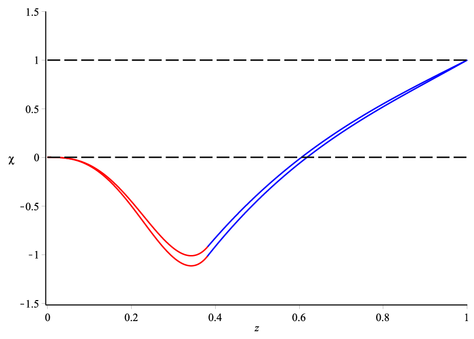
It is worth while to emphasize that the matching point $z_{\epsilon}$ is not a fixed constant but a dynamical variable depending on the temperature, the chemical potential as well as the quark mass through Eq. (3.73). (Without loss of generality, the $z_{\epsilon}$ is linear with the black hole horizon because of the dimensional analysis, so we anchor the $z_{\epsilon}=\epsilon z_{H}$.) As an example, the smoothly matched solution for $z_{H}=1$ and $\mu=0,1$ are plotted in Fig. 5(a). The red part is the near boundary solution with boundary condition $\chi(0)=0$, and the blue part is the near horizon solution with the boundary condition $\chi(z_{H})=1$. The two asymptotic solutions are smoothly connected at the matching point $z_{\epsilon}\sim 0.381$. For different chemical potentials, the matching point is almost saturated in a constant as showed in Fig. 5(a).