Interplay of Flat Electronic Bands with Holstein Phonons

We use the adiabatic approximation, ignoring the $\hat{p}_{\bf i}^{2}$ term, and assume a staggered pattern of phonon displacements with the ansatz $x_{\bf i}=x_{0}-\Delta$ for sublattice A and $x_{\bf i}=x_{0}+\Delta$ for sublattice B/C. Inserting this ansatz into Eq. 1, the resulting quadratic fermion Hamiltonian can be diagonalized. Then the free energy is a function of $x_{0}$, $\Delta$ and inverse temperature $\beta$,

where

are the three fermion energy bands, and $\mathbf{k}=(k_{x},k_{y})$ are allowed momentum vectors. At a fixed temperature $T$, we determine the ($x_{0}^{*}$, $\Delta^{*}$) which minimize $F$. Results obtained by this approach will be presented in the next section.

Although much insight can be gleaned from MFT, especially concerning the possible types of order, it has a number of well-understood defects, especially an overestimate of the tendency to long range order arising from ignoring fluctuations. This is particularly evident in lattice models like the Hubbard and Holstein Hamiltonians where it fails to distinguish two separate energy scales. The first is the temperature $T\sim U$ at which local moments (in the case of repulsive interactions) or pairs (in the case of attractive interactions) form. The second is the temperature at which inter-site ordering occurs. Since the former grows linearly with the interaction strength $U$, and the latter falls as $1/U$, MFT overestimates $T_{c}$ by a far wider margin at strong coupling than in simpler classical descriptions of long range order such as the Ising model.

To provide a more accurate treatment of the electron-phonon correlations, we turn to the use of the DQMC methodologyBlankenbecler et al. 1981; Sorella et al. 1989. In this approach, the full imaginary time propagator $e^{-\beta\hat{\cal H}}$ is written as a product of incremental factors $e^{-\Delta\tau\hat{\cal H}}$. This discretization allows for the ‘Trotter’ approximation, $e^{-\Delta\tau\hat{\cal H}}\approx e^{-\Delta\tau\hat{\cal H}_{1}}e^{-\Delta\tau\hat{\cal H}_{2}}$ with $\hat{\cal H}=\hat{\cal H}_{1}+\hat{\cal H}_{2}$. The purpose of dividing up the imaginary time evolution is that the matrix elements of the individual pieces can be evaluated analytically. In particular, upon the introduction of complete sets of phonon states, the fermionic trace in the resulting quadratic form of fermionic operators can be performed, leaving a trace over a phonon field $x(\mathbf{i},\tau)$ which depends on both spatial site $\mathbf{i}$ and imaginary time slice $\tau$. The integrand has both a bosonic piece from the quantum oscillator term in $\hat{\cal H}$ and a product of two determinants (one from each spin species) which depend on $x(\mathbf{i},\tau)$. For the Holstein model, because the up and down species couple to the phonon coordinate in the same way, the determinants are identical. The fermion sign problem is absent in the resulting square of determinants. $x(\mathbf{i},\tau)$ is sampled stochastically.

DQMC treats interacting quantum Hamiltonians exactly. The sole (controlled) approximation is in the discretization of $\beta$. With the usual choices of $\Delta\tau$ the associated errors are easily made smaller than those arising from the sampling. (The exception is for local quantities like the energy and double occupancy whose statistical errors are extremely small. For these observables, a $\Delta\tau\rightarrow 0$ extrapolation is straightforward to perform.) Simulations are carried out on lattices of finite size, necessitating a finite size scaling analysis, as described below.

We focus on several local observables, the density $\rho=\langle\hat{n}_{\mathbf{i}}\rangle$ and double occupancy ${\cal D}=\langle\hat{n}_{\mathbf{i}\uparrow}\hat{n}_{\mathbf{i}\downarrow}\rangle$, and on the CDW structure factor, the Fourier transform of the real-space density-density correlation function.

where $\Delta\hat{n}_{\mathbf{i}}=\sum_{\sigma}\Delta\hat{n}_{\mathbf{i},\sigma}=\sum_{\sigma}\hat{n}_{\mathbf{i}B,\sigma}+\hat{n}_{\mathbf{i}C,\sigma}-2\hat{n}_{\mathbf{i}A,\sigma}$ is the charge density difference within a unit cell, labeled by ${\bf i}$. When only the A or B/C sublattice is occupied, corresponding to one-third or two-thirds filling, the dominant $S(\mathbf{q})$ will be $S_{\rm cdw}=S(0,0)$.

The spectral function $A(r,\omega)$ is obtained by an analytic continuation of the non-equal time Greens function

We report the Fourier transform of the spectral function at zero distance, a quantity which is the analog of the non-interacting density of states in a correlated system.

DQMC has been used to explore various properties of the attractive and repulsive Hubbard models on the Lieb LatticeIglovikov et al. 2014; Costa et al. 2016; Oliveira et al. 2019, but has not yet been used for the Holstein model.

We first explore the effect of electron phonon interaction by using the mean field theory approach described in section 3A. Since the $\lambda x_{\bf i}n_{\bf i}$ term in the mean field Holstein Hamiltonian can be viewed as a chemical potential $\lambda x_{\bf i}$ acting on site i, a nonzero bond dimerization $\Delta$ implies a staggered pattern of electron density, i.e. a CDW phase. We set $\mu=-\frac{\lambda^{2}}{\omega_{0}^{2}}$ so that the lattice is half filled. The corresponding $x_{0}=-\frac{\lambda}{\omega_{0}^{2}}$.

The value $\Delta^{*}$ which minimizes ${\cal F}$ is plotted as a function of temperature $T$ in Fig. 4. For $T>T_{c}\sim 1.9\,t$, the order parameter $\Delta^{*}=0$ and there are equal sublattice densities $\rho_{A}=\rho_{B/C}=1/2$ per spin. (See also Fig. 5.) Below $T_{c}$, we find there is a degenerate pair of nonzero solutions $\pm\Delta^{*}$, and distinct densities $\rho_{A};\,\rho_{B/C}$ on the two sublattices. We denote the densities per spin on the whole lattice, i.e. averaged over sublattices, $(\rho_{A}+2\rho_{B/C})\,/\,3$, by $1/2\pm d\rho$. The two signs are associated with the two signs $\pm\Delta^{*}$. A change in sign of $\Delta^{*}$ can be viewed an interchange $A\leftrightarrow B/C$ of the high and low occupation sublattices. Since the numbers of sites in the two sublattices are unequal, this also shifts the density on the whole lattice (unlike the more conventional cases of square and honeycomb bipartite lattices).

Perfect CDW order, in which $1/2\pm d\rho=1/3;\,2/3$, and $(\rho_{A};\,\rho_{B/C})=(1,0)$ or $(0,1)$, requires the absence of both thermal ($T\rightarrow 0$) and quantum ($\lambda^{2}/\omega_{0}^{2}\rightarrow\infty$) fluctuations. In Fig. 4, $\Delta^{*}$ increases to a maximal value $\Delta^{*}\sim 1.85$ at zero temperature. $\Delta^{*}=2$ would yield a perfect CDW pattern. That $\Delta^{*}<2$ reflects the presence of some residual quantum fluctuations: $\lambda^{2}/\omega_{0}^{2}$ is finite. Not surprisingly, in Fig. 5, the density per spin $\rho_{B/C}$ (red) is closer to the perfect CDW state, $\rho=0$ (empty) or $\rho=1$ (doubly occupied), than the density $\rho_{A}$ (blue). This is because sites A have twice as many nearest neighbors as sites B/C. The larger number of hoppings $t$ produce more quantum fluctuations.

All MFT results presented in this paper are obtained on a $3\times(40\times 40)$ Lieb lattice with a dimensionless electron phonon coupling constant $\lambda_{D}\equiv\frac{\lambda^{2}}{\omega_{0}^{2}W}=\sqrt{2}/2$. Here $W=4\sqrt{2}t$ is the fermion band width for a Lieb lattice in the noninteracting limit. We will see later the MFT $T_{c}\sim 1.9\,t$ is more than an order of magnitude higher than the $T_{c}$ given by DQMC.

For different chemical potential $\mu$, we follow the same steps to determine $(x_{0}^{*},\Delta^{*})$ minimizing the free energy and find $\Delta^{*}>0$ ($\rho=1/3$ CDW pattern) when $\mu<-\frac{\lambda^{2}}{\omega_{0}^{2}}$; $\Delta^{*}<0$ ($\rho=2/3$ CDW pattern) when $\mu>-\frac{\lambda^{2}}{\omega_{0}^{2}}$. The electron density can be obtained by $n=\sum_{\alpha,\mathbf{k}}\frac{1}{1+e^{\beta\epsilon_{\alpha}}}$. Figure 6 shows the density $\rho$ per spin as a function of chemical potential $\mu$. As temperature is lowered, plateaus at $\rho=1/3$ and $\rho=2/3$ develop, indicating that a 1/3 filling CDW pattern and its partner at 2/3 filling, extend over a finite range of $\mu$, which is consistent with the DQMC results below. A similar phenomenon is also observed in the ‘$t-V$ model’ of spinless fermions interacting with a nearest neighbor repulsion on a Lieb lattice.Bercx et al. 2017.

We now turn to DQMC results. We begin with the spectral function in Fig. 7. At high temperatures (small $\beta$) $A(\omega=0)$ is non-zero. A gap is fully formed at $\beta_{c}\,t\sim 6$, suggesting a transition to an insulating CDW phase.

A more accurate determination of the location of the CDW transition is obtained by a finite size scaling analysis of $S_{\rm cdw}$. Because the low temperature phase involves occupying one of two spatial sublattices, it breaks a ${\cal Z}_{2}$ symmetry, and therefore the transition should be in the Ising universality class. Using the known 2D Ising critical exponents $\nu=1$ and $\gamma/\nu=7/4$ yields the finite size scaling plots of Fig.8. We find $\beta_{c}\,t=6.4\pm 0.1$. If we eschew this knowledge and instead vary the critical exponents and minimize the scatter of the data collapse plot, the resulting $\gamma/\nu$ is within 5% of the 2D Ising value. An example of such an analysis (for the honeycomb lattice) is given in Zhang et al. 2019.

The real space density correlations $c(\mathbf{r})$ provide additional insight into the nature of the CDW order. Figures 9 and 10 give color intensity plots of $c(\mathbf{r})$ for different temperatures and initializations of the phonon displacement $x(\mathbf{i},\tau)$. More specifically, if we start the phonon displacement at $x_{0}-\Delta$ (with $\Delta>0$), the fermion density on that site tends to be high, while a displacement $x_{0}+\Delta$ is associated with a low density. At high temperatures, the correlations are independent of the starting configuration and $c(\mathbf{r})=\langle n_{\mathbf{i+r}}n_{\mathbf{i}}\rangle=\langle n_{\mathbf{i+r}}\rangle\langle n_{\mathbf{i}}\rangle\sim 1$. Short range correlations begin to develop at $\beta\,t\sim 6$ and a strong alternation between $c(\mathbf{r})\sim 4$, where $\mathbf{r}$ connects a pair of doubly occupied sites, and $c(\mathbf{r})\sim 0$, where one of the sites is empty, becomes apparent. In the case of the initialization in the $\rho=1/3$ state (Fig. 9) with only sublattice A sites occupied, density correlations referenced to an A site (top panel) show the alternation, whereas if referenced to an unoccupied B site (bottom panel) all $c(\mathbf{r})$ become small. Conversely, for initialization in the $\rho=2/3$ state (Fig. 10) with sublattice B,C sites occupied, density correlations referenced to a B site (bottom panel) show the alternation, whereas if referenced to an unoccupied A site (top panel) all $c(\mathbf{r})$ become small.

Another way to examine the evolution into one of two possible ground states, characterized by distinct densities, is to begin several simulations with constant density $\rho=1/2$ per spin, and examine the final densities achieved. Figure 11 shows the result for four such simulations. At small $\beta$ the lattice remains half-filled, but as $\beta$ increases the lattice falls into either the $\rho=1/3$ or the $\rho=2/3$ minimum. The tendency for this splitting begins about $\beta\sim 5$. For $5\lesssim\beta\lesssim 9$ the data tend to fill the region between the upper and lower densities. This happens because at finite temperatures and on finite lattices, tunneling between the two minima can occur in the course of a simulation. Depending on the relative amount of time spent at $\rho=1/3$ and $\rho=2/3$, the average density can take different values. For $\beta\gtrsim 9$ very little tunneling occurs, and the data instead lie on just one of the two bounding lines. Note that the order parameter depends on $\beta$ so that the increasing width of the $\rho$ curves reflects the growth of the CDW order parameter below $\beta_{c}$.

It is important to emphasize a subtlety of the physics. Although the simulations of Fig. 11 were done at the chemical potential $\mu=-\lambda^{2}/\omega_{0}^{2}$ which should give $\rho=1/2$ per spin by particle-hole symmetry, the symmetry is broken and there are two low temperature phases with $\rho=1/3$ and $\rho=2/3$. This is precisely analogous to a simulation of a magnetic (e.g. Ising) model at zero external field. Although symmetry demands magnetization $M=0$, below $T_{c}$ there are two phases with $M=\pm M_{*}$.

Plots of the density $\rho$ versus chemical potential $\mu$ (Fig. 12) also reveal the CDW phase. At high temperatures $\rho$ evolves smoothly between the empty and a fully-packed limits, transiting half-filling at the particle-hole symmetry point $\mu=-\lambda^{2}/\omega_{0}^{2}$. At temperatures below the CDW transition, a plateau develops in which the compressibility $\kappa=d\rho/d\mu$ vanishes. However, unlike the situation on a bipartite lattice in which each sublattice has equal numbers of particles, the plateau is bifurcated by an abrupt jump as the system transitions from occupation of the minority to majority sublattice.

Figure 13 is similar to Fig. 11 except showing the double occupancy ${\cal D}$. At low $\beta$ (high $T$), ${\cal D}=\langle n_{\mathbf{i}\uparrow}n_{\mathbf{i}\downarrow}\rangle\sim\langle n_{\mathbf{i}\uparrow}\rangle\langle n_{\mathbf{i}\downarrow}\rangle\sim 1/4$. As $T$ decreases below the pair binding scale $U_{\rm eff}=\lambda^{2}/\omega_{0}^{2}\sim 4$, pairs begin to form on half the sites (${\cal D}\sim 0.5$). At larger $\beta$ a CDW pattern emerges in which ${\cal D}=0$ or ${\cal D}=1$ depending on which sublattice is occupied.

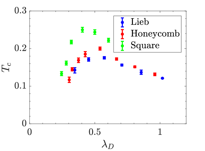
Figure 14 is the phase diagram of the Holstein model on a Lieb lattice in the plane of temperature-dimensionless coupling constant. We also compare to several other geometries. A striking feature of the plot is that the honeycomb and Lieb lattice values are so close. Naively, one might have argued that the delta-function divergence of the Lieb lattice flat band density of states would lead to a large $T_{c}$, especially when compared to the semi-metallic case of the honeycomb lattice. However, the explanation is clear- The Lieb lattice CDW order really occurs for $\rho=1/3$ and $\rho=2/3$, where it has Dirac cones much like the honeycomb lattice. Thus the only difference is that the honeycomb lattice coordination number $z=3$, whereas for the Lieb geometry the average coordination number is slightly smaller $\bar{z}=2/3(2)+1/3(4)=8/3$. Obtaining the weak coupling behavior of $T_{c}$ is a nontrivial analytic calculation. It has been done for the 2D square lattice, yielding good agreement with DQMC simulations similar to those reported hereFreericks and Scalapino 1994.

References

- Derzhko et al. (2015) O. Derzhko, J. Richter, and M. Maksymenko, “Strongly correlated flat-band systems: The route from Heisenberg spins to Hubbard electrons,” Int. J. of Mod. Phys. B 29, 1530007 (2015).
- Daniel Leykam and Alexei Andreanov and Sergej Flach (2018) Daniel Leykam and Alexei Andreanov and Sergej Flach, “Artificial flat band systems: from lattice models to experiments,” Advances in Physics: X 3, 1473052 (2018), https://doi.org/10.1080/23746149.2018.1473052 .
- Sutherland (1986) Bill Sutherland, “Localization of electronic wave functions due to local topology,” Phys. Rev. B 34, 5208–5211 (1986).
- Lieb (1989) Elliott H. Lieb, “Two theorems on the Hubbard model,” Phys. Rev. Lett. 62, 1201–1204 (1989).
- Mielke (1991a) A Mielke, “Ferromagnetic ground states for the Hubbard model on line graphs,” J. Phys. A: Math. Gen. 24, L73 (1991a).
- Mielke (1991b) A Mielke, “Ferromagnetism in the Hubbard model on line graphs and further considerations,” Journal of Physics A: Mathematical and General 24, 3311 (1991b).
- Tasaki (1992) Hal Tasaki, “Ferromagnetism in the Hubbard models with degenerate single-electron ground states,” Phys. Rev. Lett. 69, 1608–1611 (1992).
- Tasaki (1998) Hal Tasaki, “From Nagaoka’s Ferromagnetism to Flat-Band Ferromagnetism and Beyond,” Prog. Theor. Phys. 99, 489–548 (1998).
- Julku et al. (2016) Aleksi Julku, Sebastiano Peotta, Tuomas I. Vanhala, Dong-Hee Kim, and Päivi Törmä, “Geometric Origin of Superfluidity in the Lieb-Lattice Flat Band,” Phys. Rev. Lett. 117, 045303 (2016).
- Kumar et al. (2019) Pramod Kumar, Tuomas I. Vanhala, and Päivi Törmä, “Magnetization, -wave superconductivity, and non-Fermi-liquid behavior in a crossover from dispersive to flat bands,” Phys. Rev. B 100, 125141 (2019).
- (11) Kukka-Emilia Huhtinen and Päivi Törmä, “Insulator-pseudogap crossover in the Lieb lattice,” arXiv:2007.05118 .
- Swain and Karmakar (2020) Nyayabanta Swain and Madhuparna Karmakar, “Strain-induced superconductor-insulator transition on a Lieb lattice,” Phys. Rev. Research 2, 023136 (2020).
- Huber and Altman (2010) S. D. Huber and E. Altman, “Bose condensation in flat bands,” Phys. Rev. B 82, 184502 (2010).
- Tovmasyan et al. (2013) M. Tovmasyan, E. Van Nieuwenburg, and S. D. Huber, “Geometry induced pair condensation,” Phys. Rev. B 88, 220510R (2013).
- Iglovikov et al. (2014) V. I. Iglovikov, F. Hébert, B. Grémaud, G. G. Batrouni, and R. T. Scalettar, “Superconducting transitions in flat-band systems,” Phys. Rev. B 90, 094506 (2014).
- Parameswaran et al. (2013) S.A. Parameswaran, R. Roy, and S. Sondhi, “Fractional quantum Hall physics in topological flat bands,” Comptes Rendus Physique 14, 816 (2013).
- Bergholtz and Liu (2013) E. Bergholtz and Z. Liu, “Topological Flat Band Models and Fractional Chern Insulators,” Int. J. of Mod. Phys. B 27, 1330017 (2013).
- Takayoshi et al. (2013) S. Takayoshi, H. Katsura, N. Watanabe, and H. Aoki, “Phase diagram and pair Tomonaga-Luttinger liquid in a Bose-Hubbard model with flat bands,” Phys. Rev. A 88, 063613 (2013).
- Grémaud and Batrouni (2017) Benoît Grémaud and G. George Batrouni, “Haldane phase on the sawtooth lattice: Edge states, entanglement spectrum, and the flat band,” Phys. Rev. B 95, 165131 (2017).
- Cao et al. (2018a) Y. Cao, V. Fatemi, A. Demir, S. Fang, S. Tomarken, J. Luo, J. Sanchez-Yamagishi, K. Watanabe, T. Taniguchi, E. Kaxiras, R. Ashoori, and P. Jarillo-Herrero, “Correlated insulator behaviour at half-filling in magic-angle graphene superlattices,” Nature 556, 80 (2018a).
- Cao et al. (2018b) Y. Cao, V. Fatemi, S. Fang, K. Watanabe, T. Taniguchi, E. Kaxiras, and P. Jarillo-Herrero, “Un-conventional superconductivity in magic-angle graphene super-lattices,” Nature 556, 43 (2018b).
- Guo et al. (2018) H. Guo, X. Zhu, S. Feng, and R. Scalettar, “Pairing symmetry of interacting fermions on twisted bilayer graphene superlattice,” Phys. Rev. B 97, 235453 (2018).
- Pinto et al. (2020) A. Pinto, N. Frazao, D. Azevedo, and F. Moraes, “Evidence for flat zero-energy bands in bilayer graphene with a periodic defect lattice,” Physica E 119, 113987 (2020).
- Lee et al. (2020) J. M. Lee, C. Geng, J.W. Park, M. Oshikawa, S. Lee, H. Yeom, and G. Cho, “Stable Flatbands, Topology, and Superconductivity of Magic Honeycomb Networks,” Phys. Rev. Lett. 124, 137002 (2020).
- Shen et al. (2020) C. Shen, Y. Chu, Q-S. Wu, N. Li, S. Wang, Y. Zhao, J. Tang, J. Liu, J. Tian, K. Watanabe, T. Taniguchi, R. Yang, Z. Meng, D. Shi, O. Yazyev, and G. Zhan, “Correlated states in twisted double bilayer graphene,” Nature Physics 16, 520 (2020).
- Guzmán-Silva et al. (2014) D Guzmán-Silva, C Mejía-Cortés, M A Bandres, M C Rechtsman, S Weimann, S Nolte, M Segev, A Szameit, and R A Vicencio, “Experimental observation of bulk and edge transport in photonic Lieb lattices,” New Journal of Physics 16, 063061 (2014).
- Mukherjee et al. (2015) Sebabrata Mukherjee, Alexander Spracklen, Debaditya Choudhury, Nathan Goldman, Patrik Öhberg, Erika Andersson, and Robert R. Thomson, “Observation of a Localized Flat-Band State in a Photonic Lieb Lattice,” Phys. Rev. Lett. 114, 245504 (2015).
- Noda et al. (2014) Kazuto Noda, Kensuke Inaba, and Makoto Yamashita, “Flat-band ferromagnetism in the multilayer Lieb optical lattice,” Phys. Rev. A 90, 043624 (2014).
- Xia et al. (2016) Shiqiang Xia, Yi Hu, Daohong Song, Yuanyuan Zong, Liqin Tang, and Zhigang Chen, “Demonstration of flat-band image transmission in optically induced Lieb photonic lattices,” Opt. Lett. 41, 1435–1438 (2016).
- Santos et al. (2004) L. Santos, J.I. Cirac M.A. Baranov, H.-U. Everts, H. Fehrmann, and M. Lewenstein, “Atomic Quantum Gases in Kagome Lattices,” Phys. Rev. Lett. 93, 030601 (2004).
- Wu et al. (2007) C. Wu, D. Bergman, L. Balents, and S. Das Sarma, “Flat Bands and Wigner Crystallization in the Honeycomb Optical Lattice,” Phys. Rev. Lett. 99, 070401 (2007).
- Li and Johnston (2020) S. Li and S. Johnston, “Quantum Monte Carlo study of lattice polarons in the two-dimensional three-orbital Su–Schrieffer–Heeger model,” NPJ Quantum Mater. 5, 40 (2020).
- Feng et al. (2020) Chunhan Feng, Huaiming Guo, and Richard T. Scalettar, “Charge density waves on a half-filled decorated honeycomb lattice,” Phys. Rev. B 101, 205103 (2020).
- Holstein (1959) T Holstein, “Studies of polaron motion: Part I. The molecular-crystal model,” Annals of Physics 8, 325 (1959).
- Freericks et al. (1993) J. K. Freericks, M. Jarrell, and D. J. Scalapino, “Holstein model in infinite dimensions,” Phys. Rev. B 48, 6302–6314 (1993).
- Romero et al. (1999) A.H. Romero, D.W. Brown, and K. Lindenberg, “Effects of dimensionality and anisotropy on the Holstein polaron,” Phys. Rev. B 60, 14080 (1999).
- Ku et al. (2002) L.C. Ku, S.A. Trugman, and J. Bonca, “Dimensionality effects on the Holstein polaron,” Phys. Rev. B 65, 174306 (2002).
- Hohenadler et al. (2004) M. Hohenadler, H. G. Evertz, and W. von der Linden, “Quantum Monte Carlo and variational approaches to the Holstein model,” Phys. Rev. B 69, 024301 (2004).
- Marchand and Berciu (2013) Dominic J. J. Marchand and Mona Berciu, “Effect of dispersive optical phonons on the behavior of a Holstein polaron,” Phys. Rev. B 88, 060301 (2013).
- Scalettar et al. (1989a) R. T. Scalettar, N. E. Bickers, and D. J. Scalapino, “Competition of pairing and Peierls–charge-density-wave correlations in a two-dimensional electron-phonon model,” Phys. Rev. B 40, 197–200 (1989a).
- Marsiglio (1992) F. Marsiglio, “Eliashberg theory of the critical temperature and isotope effect. Dependence on bandwidth, band-filling, and direct Coulomb repulsion,” J. Low. Temp. Phys. 87, 659 (1992).
- von der Linden et al. (1995) W. von der Linden, E. Berger, and P. Valásek, “The Hubbard-Holstein model,” J. Low Temp. Phys. 99, 517 (1995).
- Alexandrov (2001) A. S. Alexandrov, “Breakdown of the Migdal-Eliashberg theory in the strong-coupling adiabatic regime,” Europhys. Lett. 56, 92–98 (2001).
- (44) Andrey V. Chubukov, Artem Abanov, Ilya Esterlis, and Steven A. Kivelson, “Eliashberg theory of phonon-mediated superconductivity – when it is valid and how it breaks down,” arXiv:2004.01281 .
- Dee et al. (2020) Philip M Dee, Jennifer Coulter, Kevin G Kleiner, and Steven Johnston, “Relative importance of nonlinear electron-phonon coupling and vertex corrections in the holstein model,” Communications Physics 3, 1–7 (2020).
- Noack et al. (1991) R.M. Noack, D.J. Scalapino, and R.T. Scalettar, “CDW and Pairing Susceptibilities in a Two Dimensional Electron–Phonon Model,” Phys. Rev. Lett. 66, 778 (1991).
- Vekić et al. (1992) M. Vekić, R.M. Noack, and S.R. White, “Charge-density waves versus superconductivity in the Holstein model with next-nearest-neighbor hopping,” Phys. Rev. B 46, 271 (1992).
- (48) O. Bradley and R. Scalettar, work in progress .
- Scalettar et al. (1989b) R. T. Scalettar, D. J. Scalapino, R. L. Sugar, and D. Toussaint, “Phase diagram of the half-filled 3D Hubbard model,” Phys. Rev. B 39, 4711–4714 (1989b).
- Vekić and White (1993) M. Vekić and S. R. White, “Gap formation in the density of states for the Holstein model,” Phys. Rev. B 48, 7643–7650 (1993).
- Weber and Hohenadler (2018) Manuel Weber and Martin Hohenadler, “Two-dimensional Holstein-Hubbard model: Critical temperature, Ising universality, and bipolaron liquid,” Phys. Rev. B 98, 085405 (2018).
- Costa et al. (2018) N. C. Costa, M. V. Araújo, J. P. Lima, T. Paiva, R. R. dos Santos, and R. T. Scalettar, “Compressible ferrimagnetism in the depleted periodic Anderson model,” Phys. Rev. B 97, 085123 (2018).
- Zhang et al. (2019) Y.X. Zhang, W.T. Chiu, N.C. Costa, G.G. Batrouni, and R.T. Scalettar, “Charge Order in the Holstein Model on a Honeycomb Lattice,” Phys. Rev. Lett. 122, 077602 (2019).
- Cohen-Stead et al. (2019) B. Cohen-Stead, N.C. Costa, E. Khatami, and R.T. Scalettar, “Effect of Strain on Charge Density Wave Order in the Holstein Model,” Phys. Rev. B 100, 045125 (2019).
- Chen et al. (2019) C. Chen, X.Y. Xu, Z.Y. Meng, and M. Hohenadler, “Charge-Density-Wave Transitions of Dirac Fermions Coupled to Phonons,” Phys. Rev. Lett. 122, 077601 (2019).
- (56) B. Xiao, N.C. Costa, E. Khatami, G.G. Batrouni, and R.T. Scalettar, “Charge Density Wave and Superconductivity in the Disordered Holstein Model,” arXiv:1910.08703 .
- Chen et al. (2018) Chuang Chen, Xiao Yan Xu, Junwei Liu, George Batrouni, Richard Scalettar, and Zi Yang Meng, “Symmetry-enforced self-learning Monte Carlo method applied to the Holstein model,” Phys. Rev. B 98, 041102 (2018).
- Beyl et al. (2018) Stefan Beyl, Florian Goth, and Fakher F. Assaad, “Revisiting the hybrid quantum Monte Carlo method for Hubbard and electron-phonon models,” Phys. Rev. B 97, 085144 (2018).
- Batrouni and Scalettar (2019a) G. G. Batrouni and Richard T. Scalettar, “Langevin Simulations of a Long Range Electron Phonon Model,” Phys. Rev. B 99, 035114 (2019a).
- Batrouni and Scalettar (2019b) G. G. Batrouni and Richard T. Scalettar, “Quantum Monte Carlo with the Langevin Equation: Coupled Bose-Fermi Systems,” Comm. Comp. Phys. 1290, 012004 (2019b).
- (61) Y. Zhang, C. Feng, G.G. Batrouni, and R. Scalettar, work in progress .
- Blankenbecler et al. (1981) R. Blankenbecler, D. J. Scalapino, and R. L. Sugar, “Monte Carlo calculations of coupled boson-fermion systems. I,” Phys. Rev. D 24, 2278–2286 (1981).
- Sorella et al. (1989) S. Sorella, S. Baroni, R. Car, and M. Parinello, “A Novel Technique for the Simulation of Interacting Fermion Systems,” Europhys. Lett. 8, 663 (1989).
- Costa et al. (2016) Natanael C. Costa, Tiago Mendes-Santos, Thereza Paiva, Raimundo R. dos Santos, and Richard T. Scalettar, “Ferromagnetism beyond Lieb’s theorem,” Phys. Rev. B 94, 155107 (2016).
- Oliveira et al. (2019) W. S. Oliveira, N. C. Costa, J. Pimentel de Lima, and Raimundo R. dos Santos, “Classical and quantum percolation on the Lieb lattice,” (2019), unpublished.
- Bercx et al. (2017) Martin Bercx, Johannes S. Hofmann, Fakher F. Assaad, and Thomas C. Lang, “Spontaneous particle-hole symmetry breaking of correlated fermions on the Lieb lattice,” Phys. Rev. B 95, 035108 (2017).
- Freericks and Scalapino (1994) J. K. Freericks and D. J. Scalapino, “Weak-coupling expansions for the attractive holstein and hubbard models,” Phys. Rev. B 49, 6368–6371 (1994).