Capillary Hysteresis and Gravity Segregation in Two Phase Flow Through Porous Media
Abstract
We study the gravity driven flow of two fluid phases in a one dimensional homogeneous porous column when history dependence of the pressure difference between the phases (capillary pressure) is taken into account. In the hyperbolic limit, solutions of such systems satisfy the Buckley-Leverett equation with a non-monotone flux function. However, solutions for the hysteretic case do not converge to the classical solutions in the hyperbolic limit in a wide range of situations. In particular, with Riemann data as initial condition, stationary shocks become possible in addition to classical components such as shocks, rarefaction waves and constant states. We derive an admissibility criterion for the stationary shocks and outline all admissible shocks. Depending on the capillary pressure functions, flux function and the Riemann data, two cases are identified a priori for which the solution consists of a stationary shock. In the first case, the shock remains at the point where the initial condition is discontinuous. In the second case, the solution is frozen in time in at least one semi-infinite half. The predictions are verified using numerical results.
1 Introduction
In this paper we investigate gravity driven flow of two fluid phases through a homogeneous one-dimensional porous column. We are concerned with the special case in which the length of the column is large and no injection of fluid is present (i.e. the total flow is zero). The corresponding mathematical model uses the well-known Buckley-Leverett equation, see [9]. In dimensionless form it reads
| (1.1) |
Here is the saturation of the wetting phase and the fractional flow function of which a typical sketch is shown in Figure 1 (left). The space coordinate is and denotes time. We solve (1.1) for and , where we prescribe at the Riemann condition
| (1.2) |
Solutions of (1.1)–(1.2) are generally non-unique [14, Chapter 1]. To find the physically relevant solution, we replace (1.1) by the capillary Buckley-Leverett equation
| (1.3) |
and study the limit . In (1.3), is the pressure difference between the fluid phases and is the dimensionless capillary number which scales inversely with the length of the domain (reference length). Hence for large domains, (1.1) is approximated by (1.3). A detailed derivation is given in Section 2.
To solve (1.3) a relation between and is assumed. In the standard equilibrium approach, one uses
| (1.4) |
where is a capillary pressure function [9].
For , let denote the solution of (1.2)–(1.4). The hyperbolic limit as yields the well known Buckley-Leverett solution of (1.1)–(1.2), comprising of constant states separated by shocks and rarefaction waves [22, 15, 14]. In particular, shocks can be seen as the limit of smooth, monotone travelling waves which become steeper as [14, 15, 31]. It is also known that the hyperbolic limit solution is independent of the actual shape of the capillary pressure as long as the approximating equation (1.3) is of convection-diffusion type [14, Chapter 3].


However, there are other more realistic capillary pressure expressions for which the limiting solution does inherit some properties of the vanishing capillarity. This was studied in detail in [34, 32, 30, 19] for the case where (1.4) is replaced by the non-equilibrium expression
where is a relaxation parameter called dynamic capillarity coefficient which attributes to saturation overshoot [33, 20, 17].
In this paper we investigate the effect of hysteresis in the capillary pressure. Since is a single valued function of saturation only, it does not contain any information about the history or directionality of the process. In particular, it does not distinguish between imbibition and drainage. No hysteretic effects are present in (1.4). However, hysteresis is known to occur in multi-phase porous media flow. This was first observed by Haines in 1930 and has been verified since by numerous experiments, some notable examples being [21, 35]. An overview of different hysteresis models from the mathematical, modelling and physical perspective can be found in [28, 8, 16].
In our approach we replace (1.4) by the following hysteresis description. Let
denote the imbibition and drainage capillary pressure functions, typical examples being shown in Figure 1 (right), and let
be the hysteresis region in the -plane, as indicated in Figure 1 (right). We restrict ourselves to the well-known play-type hysteresis model, first proposed in [6], which relates and via the relation
| (1.5) |
The play-type model assumes that switching from drainage to imbibition, or vice versa, occurs only along vertical scanning curves. For the rest of the study the state when and consequently will be referred to as the undetermined state of the system, whereas (consequently ) and () will refer to the imbibition and drainage states, respectively. Other models, such as the Lenhard-Parker model [23] and the extended play-type hysteresis model [8, 18] assume a more complex relation between and when . We comment on the consequences of such models in Remark 4.2.
The purpose of this paper is to construct solutions of the Riemann problem (1.1)–(1.2) that arise as the hyperbolic limit () of (1.2)–(1.3) and (1.5). We demonstrate that the occurrence of hysteresis in the vanishing capillary term, i.e. using (1.5) instead of (1.4), gives solutions that are significantly different specially when is close to and is close to . In particular, a stationary discontinuity occurs at the location where the initial condition is discontinuous. This is illustrated in Figure 2. The magnitude of the jump depends on the difference , as will be discussed later.
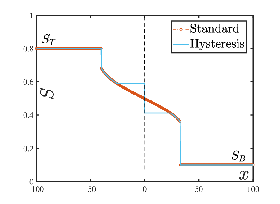
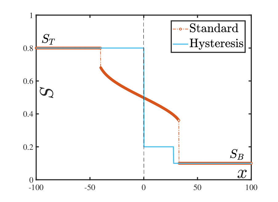
This behaviour was mentioned briefly in Section 3.5 of [19]. A stationary discontinuity in saturation for the classical problem (with no hysteresis) was also predicted in [2] at the interface between two semi-infinite halves having different and functions. However, the directionality imposed by hysteresis demands an extension of their results. The saturation discontinuity has major practical importance as the saturation distribution can change considerably if hysteresis is present, as is evident from Figure 2.
Remark 1.1 (Vanishing capillarity method).
In the mathematical literature, the method of finding solutions of equations such as (1.1) by passing to the limit in (1.3) is called the vanishing viscosity method, and was studied in classical references such as [13, 22]. In these papers, the notion of entropy was introduced, calling the vanishing viscosity solutions ‘entropy’ solutions. In the context of our application, we call the approach vanishing capillarity method, the approximate solutions for the capillarity solutions, and the limit solution the vanishing capillarity solution.
Hysteresis models have been analysed exhaustively, particularly in one spatial dimension [17]. Existence and uniqueness results for the regularised play-type model are given in [12, 27, 10, 18] and [7] respectively. A horizontal redistribution study using similarity solutions was performed in [8]. Travelling wave analysis for hysteresis was conducted for flow of water through soil in [33, 20, 5]. For the two-phase case, travelling waves were studied in [19] for monotone flux functions and vanishing capillarity solutions were derived that differ significantly from the classical ones. Non-classical solutions for non-monotone flux functions like are investigated in [29], although hysteresis is not included. In [11], examples of how hysteresis influences hyperbolic solutions in mechanics are found. The role of relative permeability hysteresis, which is not addressed in this study, in determining the hyperbolic solutions is examined in [25, 26, 4, 1]. However, the relation between and is assumed to be a linear one in these articles. In the current study, we investigate the vanishing capillarity solutions for the capillary hysteresis models in the non-monotone flux case and show that non-classical behaviour such as stationary shocks may occur. Stationary discontinuities have been studied in [2] for heterogeneous media without hysteresis and for redistribution problems (no gravity) in [8, 24] with hysteresis. The occurrence of a stationary discontinuity due to hysteresis in gravity driven flows is to our knowledge a novel observation.
We structure the paper as follows: In Section 2 the assumptions are stated and the model is derived. Using travelling wave analysis, all admissible shocks, including stationary shocks, are derived in Section 3 for the standard and the hysteresis model. Then, in Section 4, the admissible shocks are used to construct the vanishing capillarity solutions. Two cases are identified when the solutions for hysteresis deviate from the classical ones. This is determined a priori from , , , and . In the first case, the solution has a stationary discontinuity while the rest of the solution retains the structure of the classical solutions (Section 4.2.1). The second case has no classical counterparts and the solution is frozen in one of the semi-infinite halves (Section 4.2.2). Finally, in Section 5, we solve (1.2)–(1.3) and (1.5) numerically for small and show that the solution closely resembles our predictions.
2 Problem Formulation
We set-up the two-phase flow problem in a one-dimensional homogeneous porous domain. The phases are assumed to be incompressible and immiscible. There is no injection at the boundaries, making the flow purely counter-current and gravity driven, having zero total flux of the combined wetting and non-wetting phases. Following [9], we consider for each phase the mass balance equation and the corresponding Darcy Law. This yields
| (2.1a) | |||||
| (2.1b) | |||||
For each phase ( and representing the wetting and the non-wetting phases respectively), denotes the pressure, the relative permeability, the viscosity and the density. The porosity and absolute permeability are properties of the medium and are constant due to the assumption of homogeneity. Finally, gravity points in the direction of positive and is the gravitational constant. For the remainder of the study we assume that the wetting phase is denser than the non-wetting phase, i.e.,
Adding the equations in (2.1) gives
The term inside the brackets is the total flux of the combined phases. Since no-injection takes place in the column
Defining the capillary pressure and mobility ratio as
respectively, one obtains through rearrangement
| (2.2) |
To non-dimensionalise (2.1), we introduce a characteristic pressure (taken from the capillary pressure curves), a characteristic length (length of column or typical observation distance) and a characteristic time . We further define the fractional flow function
| (2.3) |
and introduce the dimensionless capillary number
| (2.4) |
Inserting (2.2) into (2.1a), choosing , and redefining the dimensional quantities as their dimensionless versions
one obtains (1.3). The Brooks-Corey model is commonly used for the relative permeability functions:
| (2.5) |
This gives the shape of as shown in Figure 1 and properties outlined in (P2). As for , either (1.4) or (1.5) is used.
For the capillary pressures and the fractional flow function, following set of properties is assumed, see Figure 1. They are consistent with experimental observations [9, 3]:
- (P1)
The capillary pressures , for , are continuously differentiable and strictly decreasing in ; and (no entry pressure).
- (P2)
The fractional flow function is smooth with . There exists such that
Moreover, there exists inflection points with such that
The assumption (P1) is consistent with the van Genuchten model for capillary pressures. For , the Brooks-Corey model (2.5) yields
| (2.6) |
3 Admissible shocks
In this section we consider shock solutions of equation (1.1) that originate from smooth solutions of (1.3). A shock is characterized by a constant left state , a constant right state and a constant speed . They are denoted by or
| (3.1) |
We call an admissible (i.e. vanishing capillarity) shock if it can be approximated, as , by smooth solutions of (1.3) [15, 14]. To investigate this, we consider a special class of solutions of (1.3) in the form of travelling waves:
| (3.2) |
Here is the saturation profile, the capillary pressure profile and the wave-speed. We consider profiles that satisfy for the saturation
| (3.3) |
and for the pressure
| (3.4) |
Clearly, if a smooth profile (3.2) exists and satisfies (3.3), then
Substituting (3.2) into (1.3) gives
| (3.5) |
where primes denote differentiation. Integrating this expression yields
| (3.6) |
If satisfies (3.3), then (3.6) implies that has a limit for . The boundedness of pressure (3.4) then forces
| (3.7) |
Using this in (3.6) for results in
| (3.8a) | ||||
| (3.8b) | ||||
giving
| (3.9) |
Substituting and in (3.6) yields
| (3.10) |
3.1 Equilibrium case: given by (1.4)
If , equation (3.11) has a solution satisfying (3.3) if for all . Hence, the shock is admissible if is given by (3.9) and
| (3.12a) | |||
| If , the shock is admissible if (3.9) is satisfied, and | |||
| (3.12b) | |||
Conditions (3.12) are classical (Oleinik admissibility conditions), see [22, 15, 14]. To see which possible admissible shocks connect to the left or right states of the Riemann problem (1.1)–(1.2) we introduce two saturations. For (first inflection point of ), let denote the unique point where the line through is tangent to the graph of . If , we set . A similar definition gives , see Figure 3. Thus, the points and satisfy,
| (3.13) |
Applying (3.12) to Riemann problem (1.1)–(1.2), we note that if , then can serve as the right state of an admissible shock for left states between , see Figure 3. Similar for and .

3.2 Hysteretic case: given by (1.5)
If or , then any admissible shock in terms of (1.4) is also an admissible shock in terms of (1.5): To see this, fix and let (3.12) hold. Define the relation between and as
Then, separately for and , and are related through the classical relation (1.4) where is replaced by and respectively. Consequently, the existence of and solving (3.10) with boundary conditions (3.3)–(3.4) follows from Section 3.1. Observe that for all as a consequence of (3.11) and (3.12). Hence, recalling from (3.2) that and , we have
It is now straightforward to verify that satisfies the hysteresis relation (1.5) for both and . Hence, shocks that are admissible in terms of the equilibrium capillary pressure (1.4) are admissible in terms of the hysteretic capillary pressure (1.5) as well, provided . Note that the profiles depend on the functional form of , but not the resulting shock.
Observe that for , the entire approximating wave is in imbibition state since and . Hence, we also refer to the resulting shock as being in imbibition state. Similarly, for , the shock is in drainage state since and . The effects of hysteresis are only observed, if the hysteretic states ahead and behind the shock are different. This can only happen for stationary shocks having zero wave speed, i.e. . For such shocks, Rankine-Hugoniot’s expression (3.9) requires
| (3.14) |
Note that this implies
| (3.15) |
Without a loss of generality we put the stationary shock at .
3.2.1 Case A: Connection between imbibition and drainage states
Let us first consider the case
| (3.16a) | ||||
| (3.16b) | ||||
The case of in imbibition and in drainage is symmetrical. Here, the imbibition and drainage states are inherited from the approximating solutions as before.
For (3.16) to be an admissible stationary shock, must be such that
- (A1)
Relation (3.14) is satisfied.
- (A2)
- (A3)
The pressure profile satisfies
(3.17)
Let and . Then (3.17) implies
| (3.18) |
Putting in (3.10) gives
| (3.19) |
This equation implies that
| (3.20) |
In particular, , or from (3.17)
| (3.21) |
Combining (3.17) and (3.19) gives the problem
| (3.22a) | ||||
| (3.22b) | ||||
where . The unique solution of (3.22) is for all . This follows from the fact that if , then from (3.15) and hence when and when . Now suppose there exists such that . Then implying . This means that for all contradicting . Similarly, if then , yielding a contradiction as well.
Repeating this reasoning for , we conclude that the unique solution of (A1)–(A3) is
| (3.23) |
where the pair in addition to satisfying (3.14), also must satisfy due to (3.21), i.e.,
| (3.24) |
We show that based on the assumptions (P1)–(P2), a unique pair with exists that satisfies (3.24). To see this, define the function as
| (3.25) |
From (P2), the function is decreasing, continuous, and , see also Figure 4 (left). Consider the strictly increasing function for . For , we have . Since is a strictly decreasing function, for small enough one has . On the other hand, . Thus, by intermediate value theorem, there exists such that , see Figure 4 (right). Thus, we put .


Hence, shocks (i.e. ), with their end states being in imbibition and drainage, are admissible if and only if (3.24) is satisfied with
| (3.26a) | ||||
| (3.26b) | ||||
where with is the unique solution of
| (3.27) |
Connecting an imbibition state with another imbibition state demands that (3.24) be satisfied with and which has the unique solution . The same result holds for connecting a drainage state with another drainage state. Hence, no non-trivial stationary shock () exists in these cases.
3.2.2 Case B: One state undetermined
It is also possible that one of the states is undetermined (neither in imbibition nor in drainage). To demonstrate the admissibility for this case, we first assume that the left state is undetermined and the right state is in imbibition. Using in (1.5), we have that is an admissible stationary shock if
- (B1)
Relation (3.14) is satisfied.
- (B2)
- (B3)
The pressure profile satisfies
(3.28)
Following the same arguments as before, we have
| (3.29) | ||||
| (3.30) |
What remains is the problem which reads
| (3.31) | ||||
| (3.32) |
Clearly, and is a solution provided,
| (3.33a) | ||||
| (3.33b) | ||||
Hence, also in this case, condition (3.24) is satisfied. We show below that additionally (3.33b) is satisfied if
| (3.34) |
where , and the function are defined in (3.27) and (3.25) respectively. Indeed, from the definition of , if then and . From (P1) it directly follows that, . To get we consider the strictly increasing function for , see the properties of , (P1) and Figures 4 and 5 (right). The function has a zero at . This means , or . The construction is also shown in Figure 5. It is straightforward to verify that this is only case when (3.33) is satisfied.


Condition (3.34) serves as the admissibility criterion when the left state is undetermined and the right state is in imbibition. Considering all combinations, including undetermined-drainage, imbibition-undetermined, drainage-undetermined and undetermined-undetermined, the complete list of admissible stationary shocks with is given in Table 1.
| Left state | Right state | ||||
| drainage | imbibition | ||||
| imbibition | drainage | ||||
| undetermined | imbibition | ||||
| imbibition | undetermined | ||||
| undetermined | drainage | ||||
| drainage | undetermined | ||||
| undetermined | undetermined |
4 Vanishing capillarity solutions of the Buckley-Leverett equation
We construct the solution of the Riemann problem (1.1)–(1.2) with the admissibility conditions from Section 3. A solution of (1.1) is composed of constant states separated by shocks and rarefaction waves. We recall that a rarefaction wave is a smooth solution of (1.1) having the form
| (4.1) |
Then for results the equation
| (4.2) |
where
Rarefaction waves are well-defined if
| (4.3) |
We show below how to construct solutions of (1.1) with rarefaction waves satisfying (4.2) along with condition (4.3), and shocks satisfying the admissibility conditions from Section 3. For completeness, we briefly recall the classical Buckley-Leverett construction.
4.1 Classical construction
The construction of vanishing capillarity solutions for the classical case is well established, see [22, 14]. Recalling the definition of and in (3.13), we identify three cases. Since the solutions for these cases will be used in Section 4.2 to construct parts of the vanishing capillarity solution for pairs other than , we also use and in the notation:
Case I: :
In this case since . The vanishing capillarity solutions are
| (4.4a) | |||
| and with defined in (4.2), | |||
| (4.4b) | |||
Case II: :
In this case . The vanishing capillarity solutions are
| (4.5a) | |||
| and | |||
| (4.5b) | |||
Case III: :
In this case we have,
| (4.6) |
4.2 Construction with capillary hysteresis
Vanishing capillarity solution for Case I and II:
Observe that in Case I of Section 4.1 () the shock is in an imbibition state and the rarefaction wave part, if it exists, satisfies . Hence, the vanishing capillarity solution as a whole is in imbibition state. Similarly, for Case II the entire solution is in drainage state. Consequently, based on the discussions in Section 3.2 and the fact that the classical solution does not depend on the specific form of , the vanishing capillarity solutions for the capillary hysteresis model in Case I and Case II are identical to the classical ones.
Vanishing capillarity solution for Case III:
As in the classical case, we construct a solution which is in imbibition state when and drainage state when . Hence one expects to have a stationary shock at . We restrict ourselves to the case
| (4.7) |
the solution for being symmetrical. With respect to the cases A and B in Section 3.2 we divide the discussion in two parts.
4.2.1 Case
The restriction (4.7) implies that . The stationary shock at in this case must connect and . To see this, assume the contrary. Recalling Table 1, we then have
where the function and are defined in (3.25) and (3.27) respectively. For and , the vanishing capillarity solution of (1.1) is classical, and thus, given by (4.4) with . Since this is a classical solution belonging to Case I of Section 4.1, it is in imbibition state. Similarly, for and , the solution is in drainage state. However, the only admissible stationary shock connecting an right imbibition state to a left drainage state is , see Table 1. Thus, the stationary shock at connects and .
Vanishing capillarity solution:
For and ,
| (4.8a) | |||
| For and , | |||
| (4.8b) | |||
Remark 4.1 (Convergence of (4.8) to the classical solutions).
4.2.2 Case
Let be such that , or in other words
| (4.9) |
Restriction (4.7) then implies that . In this case, the stationary shock is ruled out. Otherwise, since , the classical solution for and will be in imbibition state. However, recalling Table 1, the shock is not admissible for left state in imbibition. Similarly, other possibilities are eliminated using Table 1, except the following scenario:
Vanishing capillarity solution:
for and ,
| (4.10a) | |||
| For and , | |||
| (4.10b) | |||
The vanishing capillarity solutions for the cases and are shown in Figure 6. Observe that there is no classical counterpart of (4.10). The solution plotted in Figure 2 (right) for the play-type hysteresis model is of this type.
Remark 4.2 (Generality of the results with respect to other hysteresis models).
The admissible shocks presented in Table 1 and the vanishing capillarity solutions presented in (4.8) and (4.10) are consistent with any hysteresis model that satisfies the condition
| (4.11) |
Most of the commonly used hysteresis models, including the Lenhard-Parker model [23] and the extended play-type model [8] belong to this category. The results are consistent with any model satisfying (4.11) since, the models only differ in the description of when , i.e. when the hysteretic state is undetermined. As a result, if a stationary shock connects imbibition to drainage, then the set of equations (A1)–(A3) are valid also for a model satisfying (4.11). Thus, the resulting shocks are unaltered. Similarly, (B1)–(B3) (in particular (B3)) are consistent with describing the shock when one of the states is undetermined since in this case which is allowed by (4.11). Hence, models satisfying (4.11) are consistent with admissible shocks listed in Table 1, and consequently with the vanishing capillarity solutions derived in Section 4.
5 Numerical Results
To solve (1.2), (1.5) numerically, (1.5) is usually regularised in the following way:
| (5.1) |
The relaxation parameter (dynamic capillarity coefficient) was mentioned briefly in Section 1.
We solve (1.3) and (5.1) in a domain for a large . The boundary conditions used are
| (5.2) |
The approach for solving the system (1.3), (5.1)–(5.2), is based on rearranging (5.1) to express as a function of and , and using this, to consider (1.3) as an elliptic equation for the pressure. Details of the numerical method are given in Section 5 of [19], see also the numerical sections of [20, 33]. Cell centered finite difference method with a uniform mesh is used for the computation with and representing the mesh and the time step sizes respectively. The following choices of parameters are made
These values ensure both that our parabolic solver is converging and the capillarity solutions are sufficiently close to their hyperbolic limit. Since smaller also implies that the profiles take longer to develop, we have optimized the value of so that a good approximation of the developed profile is obtained in a reasonable time.
5.1 Validation


For validating our predictions of Section 4 we use Brooks-Corey expression (2.6) for with . This gives . Van Genuchten parametrization is used here to model the capillary curves. Two choices for the imbibition and drainage curves are made. At first, we take and close to each other, i.e.,
see Figure 7 (right). In this case, direct computation shows that and . We take and implying that . The vanishing capillarity solution expected in this scenario is outlined in (4.8). It consists of shocks between – and –, rarefaction waves between – and – and a stationary shock from to at , see Figure 2 (left) and Figure 7 (left). The numerically computed solution is shown in Figure 7 (left) and in the - plane in Figure 7 (right). The numerically obtained capillary solutions are a close match to the vanishing capillarity solutions predicted. The minor differences are due to , and numerical errors. Note that the counter-current flow for stems from non-monotonicity of since the flux at is which is greater than the flux at the left boundary.


Next, we take same as before but as in Figure 1 (right):
These curves resemble experimentally obtained retention curves (see [21]) and were taken from [19]. With same as before, one has in this case. Hence, recalling Section 4.2.2, particularly (4.10), the solution is frozen for . For , there is a shock connecting and . This behaviour is mimicked by the computed capillarity solutions, see Figure 8. In this case, the total mass is still balanced since the total rate of water infiltration is (where is the shock speed introduced in (3.9)), which is precisely equal to the difference of fluxes at the left and the right boundaries.
6 Conclusion
In this paper, we considered the hyperbolic Buckley-Leverett equation (1.1) and its parabolic counterpart (1.3) for the case when the flux function is non-monotone. This occurs in gravity driven flows. In the presence of hysteresis, represented by (1.5), the hyperbolic (vanishing capillarity) limit of solutions to (1.3) differs from the classical solution obtained through the equilibrium expression (1.4). In particular, a solution to the Riemann problem (1.1)–(1.2) has a stationary shock at if the left () and the right () states lie in the increasing and decreasing parts of the flux function respectively, or vice versa. The hysteretic states on the left and right become different in this case and thus, different capillary relations are used. Using travelling wave solutions, an admissibility (entropy) condition (3.24) is derived for stationary shocks. The condition states that the flux function and the pressure corresponding to the hysteretic state of the system, remain continuous across the shock. It is then used to derive all admissible shocks. They are listed in Table 1. The shocks are classified into two categories. The first (Case A) connects imbibition states to drainage states, and the second (Case B) has one of the states undetermined.
Depending on the values of the Riemann data with respect to characteristic points that are easily computable a-priori from and the capillary curves, two possibilities are identified (corresponding to Case A and Case B) when the stationary shocks occur. The vanishing capillarity solutions for these cases are given by (4.8) and (4.10). Interestingly, the solution (4.10) remains frozen in time in one of the halves and thus, differs significantly from the classical solution. To our knowledge, this is a novel observation. The predictions were validated using numerical experiments.
Acknowledgment
K. Mitra acknowledges the support from INRIA Paris through the ERC Gatipor grant. Parts of the research for K. Mitra were also funded by TU Dortmund University, Shell–NWO (grant 14CSER016) and Hasselt University (grant BOF17BL04). C.J. van Duijn is supported by the Darcy Center of Eindhoven University of Technology and Utrecht University. The authors would like to thank Prof. Sorin Pop for many fruitful discussions on the topic.
References
- [1] E. Abreu and W. Lambert. Computational modeling technique for numerical simulation of immiscible two-phase flow problems involving flow and transport phenomena in porous media with hysteresis. In AIP Conference Proceedings 4, volume 1453, pages 141–146. American Institute of Physics, 2012.
- [2] B. Andreianov and C. Cancès. Vanishing capillarity solutions of Buckley–Leverett equation with gravity in two-rocks’ medium. Computational Geosciences, 17(3):551–572, 2013.
- [3] J. Bear. Hydraulics of groundwater. McGraw-Hill International Book Co., 1979.
- [4] P. Bedrikovetsky, D. Marchesin, and P.R. Ballin. Mathematical model for immiscible displacement honouring hysteresis. In SPE Latin America/Caribbean Petroleum Engineering Conference. Society of Petroleum Engineers, 1996.
- [5] E.E. Behi-Gornostaeva, K. Mitra, and B. Schweizer. Traveling wave solutions for the Richards equation with hysteresis. IMA Journal of Applied Mathematics, 84(4):797–812, 2019.
- [6] A.Y. Beliaev and S.M. Hassanizadeh. A theoretical model of hysteresis and dynamic effects in the capillary relation for two-phase flow in porous media. Transport in Porous Media, 43(3):487–510, 2001.
- [7] X. Cao and I.S. Pop. Two-phase porous media flows with dynamic capillary effects and hysteresis: Uniqueness of weak solutions. Computers & Mathematics with Applications, 69(7):688 – 695, 2015.
- [8] C.J. van Duijn and K. Mitra. Hysteresis and horizontal redistribution in porous media. Transport in Porous Media, 122(2):375–399, 2018.
- [9] R. Helmig. Multiphase flow and transport processes in the subsurface: a contribution to the modeling of hydrosystems. Springer-Verlag, 1997.
- [10] J. Koch, A. Rätz, and B. Schweizer. Two-phase flow equations with a dynamic capillary pressure. European Journal of Applied Mathematics, 24(1):49–75, 2013.
- [11] Pavel Krejcı. Hysteresis, convexity and dissipation in hyperbolic equations. Tokyo: Gakkotosho, 1996.
- [12] A. Lamacz, A. Rätz, and B. Schweizer. A well-posed hysteresis model for flows in porous media and applications to fingering effects. Advances in Mathematical Sciences and Applications, 21(2):33, 2011.
- [13] P.D. Lax. Hyperbolic systems of conservation laws and the mathematical theory of shock waves. Society for Industrial and Applied Mathematics, 1973.
- [14] P.G. LeFloch. Hyperbolic Systems of Conservation Laws: The theory of classical and nonclassical shock waves. Springer Science & Business Media, 2002.
- [15] T.P. Liu. Hyperbolic and viscous conservation laws. Society for Industrial and Applied Mathematics, 2000.
- [16] C.T. Miller, K. Bruning, C.L. Talbot, J.E. McClure, and W.G. Gray. Nonhysteretic capillary pressure in two-fluid porous medium systems: Definition, evaluation, validation, and dynamics. Water Resources Research, 55(8):6825–6849, 2019.
- [17] K. Mitra. Mathematical complexities in porous media flow. PhD thesis, Eindhoven University of Technology & Hasselt University, 2019. ISBN: 978-90-386-4845-3.
- [18] K. Mitra. Existence and properties of solutions of extended play-type hysteresis model. arXiv, arXiv:2009.03209, 2020.
- [19] K. Mitra, T. Köppl, I.S. Pop, C.J. van Duijn, and R. Helmig. Fronts in two-phase porous media flow problems: The effects of hysteresis and dynamic capillarity. Studies in Applied Mathematics, 144(4):449–492, 2020.
- [20] K. Mitra and C.J. van Duijn. Wetting fronts in unsaturated porous media: The combined case of hysteresis and dynamic capillary pressure. Nonlinear Analysis: Real World Applications, 50:316 – 341, 2019.
- [21] N.R. Morrow and C.C. Harris. Capillary equilibrium in porous materials. Society of Petroleum Engineers, 5(01):15–24, 1965.
- [22] O.A. Oleinik. Discontinuous solutions of non-linear differential equations. Uspekhi Matematicheskikh Nauk, 12(3):3–73, 1957.
- [23] J.C. Parker, R.J. Lenhard, and T. Kuppusamy. A parametric model for constitutive properties governing multiphase flow in porous media. Water Resources Research, 23(4):618–624, 1987.
- [24] J.R. Philip. Horizontal redistribution with capillary hysteresis. Water Resources Research, 27:1459–1469, 1991.
- [25] B. Plohr, D. Marchesin, P. Bedrikovetsky, and P. Krause. Modeling hysteresis in porous media flow via relaxation. Computational Geosciences, 5(3):225–256, 2001.
- [26] C.E. Schaerer, D. Marchesin, M. Sarkis, and P. Bedrikovetsky. Permeability hysteresis in gravity counterflow segregation. SIAM Journal on Applied Mathematics, 66(5):1512–1532, 2006.
- [27] B. Schweizer. The Richards equation with hysteresis and degenerate capillary pressure. Journal of Differential Equations, 252(10):5594 – 5612, 2012.
- [28] B. Schweizer. Hysteresis in porous media: Modelling and analysis. Interfaces Free Bound, 19(3):417–447, 2017.
- [29] M. Shearer, K.R. Spayd, and E.R. Swanson. Traveling waves for conservation laws with cubic nonlinearity and BBM type dispersion. Journal of Differential Equations, 259(7):3216–3232, 2015.
- [30] K. Spayd and M. Shearer. The Buckley–Leverett equation with dynamic capillary pressure. SIAM Journal on Applied Mathematics, 71(4):1088–1108, 2011.
- [31] C.J. van Duijn and J.M. de Graaf. Large time behaviour of solutions of the porous medium equation with convection. Journal of differential equations, 84(1):183–203, 1990.
- [32] C.J. van Duijn, Y. Fan, L.A. Peletier, and I.S. Pop. Travelling wave solutions for degenerate pseudo-parabolic equations modelling two-phase flow in porous media. Nonlinear Analysis: Real World Applications, 14(3):1361–1383, 2013.
- [33] C.J. van Duijn, K. Mitra, and I.S. Pop. Travelling wave solutions for the Richards equation incorporating non-equilibrium effects in the capillarity pressure. Nonlinear Analysis: Real World Applications, 41(Supplement C):232 – 268, 2018.
- [34] C.J. van Duijn, L.A. Peletier, and I.S. Pop. A new class of entropy solutions of the Buckley–Leverett equation. SIAM Journal on Mathematical Analysis, 39(2):507–536, 2007.
- [35] L. Zhuang. Advanced Theories of Water Redistribution and Infiltration in Porous Media: Experimental Studies and Modeling. PhD thesis, University of Utrecht, Dept. of Earth Sciences, 2017.