Tensor-based Multi-dimensional Wideband Channel Estimation for mmWave Hybrid Cylindrical Arrays Thanks: This work was supported by the National Natural Science Foundation of China (NSFC) under Grant 61671072. (Corresponding author: Tiejun Lv.) Z. Lin and T. Lv are with the School of Information and Communication Engineering, BUPT, Beijing, China (email: {linlzp, lvtiejun}@bupt.edu.cn). Z. Lin is also with the School of Electrical and Data Engineering, UTS, Sydney, Australia. W. Ni is with the Data 61, CSIRO, Sydney, Australia (e-mail: Wei.Ni@data61.csiro.au). J. A. Zhang and R. P. Liu are with the School of Electrical and Data Engineering, UTS, Sydney, Australia (e-mail: {Andrew.Zhang, RenPing.Liu}@uts.edu.au).

Zhipeng Lin Member, IEEE Tiejun Lv Senior Member, IEEE Wei Ni Senior Member, IEEE Affiliation: J. Andrew Zhang, Senior Member, IEEE, and Ren Ping Liu, Senior Member, IEEE

Abstract

Channel estimation is challenging for hybrid millimeter wave (mmWave) large-scale antenna arrays which are promising in 5G/B5G applications. The challenges are associated with angular resolution losses resulting from hybrid front-ends, beam squinting, and susceptibility to the receiver noises. Based on tensor signal processing, this paper presents a novel multi-dimensional approach to channel parameter estimation with large-scale mmWave hybrid uniform circular cylindrical arrays (UCyAs) which are compact in size and immune to mutual coupling but known to suffer from infinite-dimensional array responses and intractability. We design a new resolution-preserving hybrid beamformer and a low-complexity beam squinting suppression method, and reveal the existence of shift-invariance relations in the tensor models of received array signals at the UCyA. Exploiting these relations, we propose a new tensor-based subspace estimation algorithm to suppress the receiver noises in all dimensions (time, frequency, and space). The algorithm can accurately estimate the channel parameters from both coherent and incoherent signals. Corroborated by the Cramér-Rao lower bound (CRLB), simulation results show that the proposed algorithm is able to achieve substantially higher estimation accuracy than existing matrix-based techniques, with a comparable computational complexity.

Index Terms:

5G/B5G, millimeter wave, large-scale antenna array, tensor, hybrid beamformer.

I Introduction

Massive hybrid antenna arrays can balance the hardware cost and complexity of wideband millimeter wave (mmWave) transceivers in fifth generation (5G) and beyond 5G (B5G) mobile communications [1]. Wideband mmWave hybrid circular arrays are particularly interesting owing to their compact size, strong immunity to mutual coupling, and inherently symmetric structure that enables 360-degree azimuth coverage [2]. Channel parameter estimation for wideband mmWave hybrid circular arrays is challenging, due to high-dimensional parameters, large signal bandwidth, large signal propagation loss, and subsequent susceptibility to noises [3, 4, 5].

Existing channel parameter estimation algorithms (for the azimuth and elevation angles, and the propagation delay of an incident signal) have typically been matrix-based. By those matrix-based algorithms, the relations between different dimensions (i.e., domains) of the signal become obscure, because the received multi-dimensional (i.e., space, time and frequency) signals are stacked into two-dimensional matrices [6, 7]. Moreover, typical high-resolution matrix-based subspace estimation algorithms, such as multiple signal classification (MUSIC) [8] and estimation of signal parameters via rotational invariance techniques (ESPRIT) [9], were designed for narrowband systems, where channel parameters vary negligibly within the system band and are unaffected by an adverse beam squinting effect [10].

Wideband signal-subspace methods (WSSMs) [11, 12] have been used to remove the frequency dependence of array steering vectors and suppress the beam squinting effect, before applying (narrowband) subspace estimation algorithms in wideband mmWave systems. Existing incoherent WSSMs (IWSSMs) [13, 14] decompose received signals into multiple non-overlapping narrowbands, and estimate the parameters independently at each narrowband. These methods [13, 14] do not utilize the high temporal resolution offered by wideband mmWave systems. In [15, 11], coherent WSSMs (CWSSMs) map the frequency-dependent array steering matrices to a reference frequency by producing so-called focusing matrices. The generation of the focusing matrices in these methods requires initial values, and the performance of the methods is susceptible to the initial values. A variation of CWSSM, named unitary constrained array manifold interpolation (UCAMI), is proposed in [16, 3]. It eliminates the need for initial estimates and avoids focusing loss¹¹ 1 Focusing loss refers to the ratio between the array signal-to-noise ratios after and before focusing operations. Focusing loss can be avoided by constraining that the focusing matrices are unitary [11].. However, the focusing matrices of UCAMI are obtained by solving multi-dimensional optimization problems. The dimension of the problems is equal to the number of estimation parameters, and UCAMI is computationally expensive. To overcome the beam squinting effect, an approximated channel model is developed in [17] to quantize the angular space, which would introduce errors and grid mismatches leading to a degraded channel estimation accuracy. To circumvent the grid mismatch, the algorithm developed in [17] repeatedly refines the angular grid and applies compressive sensing to estimate parameters. As a result, multiple iterative reweighted least squares problems need to be solved.

Refer to caption — Fig. 1: The flow diagram of the proposed localization approach. From left to right, the four key steps are described in Section III, Section IV, Section V-C, and Sections V-A and V-B, respectively.

Tensor-based channel parameter estimations have been demonstrated to be more powerful than conventional matrix-based techniques in [18, 6, 19]. By arranging the received signals in a tensor form and applying tensor decomposition, the multi-dimensional parameters can be estimated with super-high accuracy [6, 7]. The papers [7, 20, 21, 22] present tensor-based algorithms for multi-dimensional channel parameter estimation, which preserve the multi-dimensional structure of signals and improve estimation accuracy in scatter-rich microwave-band channels. The authors of [23] and [24] exploit the sparsity of mmWave channels to further improve the estimation accuracy. However, their algorithms require an alternating-least-squares procedure with no guarantee of convergence. In addition, the algorithm in [24] is only suitable for narrowband systems with uniform rectangular arrays (URAs).

This paper presents a novel tensor-based approach for multi-dimensional wideband channel estimation in large-scale mmWave hybrid uniform cylindrical arrays (UCyAs). The key contributions of the paper are as follows:

•

We design the hybrid beamformers by using quasi-discrete Fourier transform (Q-DFT) to maintain the angular resolution of the hybrid UCyA with a reduced number of radio frequency (RF) chains. Developing and applying a low-complexity UCAMI, we suppress the beam squinting effect and enable coherent combining across the wideband. These are two salient steps for our new tensor-based parameter estimation.
•

We propose a new tensor-based subspace estimation algorithm to jointly estimate the delay and the azimuth and elevation angles of each received signal by exploiting the important shift-invariance relations in the constructed truncated higher-order singular value decomposition (HOSVD) model. The algorithm can suppress the receiver noises in all of the time, frequency, and space dimensions, and hence accurately estimate the high-dimensional channel parameters of multiple coherent or incoherent signal sources.
•

We introduce a new way to rearrange the measurement tensor of the received signals to decorrelate coherent signals at the hybrid UCyA, i.e., spatial smoothing. Coherent signals can then be separated and can be estimated independently by using the proposed tensor subspace estimation algorithm.

The steps of the proposed approach are illustrated in Fig. 1, and elaborated on in the rest of this paper. In the first step, the received signals are first synthesized by a hybrid directional beamformer, which uses Q-DFT to reduce the number of required RF chains (with a negligible cost of the channel estimation accuracy at the later stages of the technique). In other words, this step reduces the dimension of the received signals, so that the signals can be processed with much fewer RF chains (than antennas). The second step is a proposed low-complexity UCAMI, which suppresses the beam squinting effect efficiently by only optimizing the focusing matrices in the elevation angular domain. The third step is to reveal and exploit the inherent linear recurrence relations in the first mode of the measure tensor and run spatial smoothing to decorrelate the coherent signals. Finally, the new tensor-based joint delay-angle estimation algorithm is carried out to estimate the delay and azimuth and elevation angles based on the constructed truncated HOSVD model of the measure tensor.

Validated by the Cramér-Rao lower bound (CRLB), simulation results show that the proposed algorithm is able to achieve much higher accuracy than state-of-the-art matrix-based techniques for wideband mmWave hybrid UCyAs. The new tensor-based algorithms work well even when the signal-to-noise ratio (SNR) is low, credited to the effective noise suppression in all of the time, space, and frequency domains.

Different from the existing studies, e.g, [17], we develop a new low-complexity UCAMI to suppress the beam squinting effect, which does not quantize the angular space and hence no quantization error will occur. Moreover, we reveal and exploit inherent shift-invariance relations [25] in each domain/mode of the measurement tensor. As a result, our algorithm only needs to solve a one-time HOSVD of the measurement tensor to estimate the multi-dimensional parameters jointly.

The rest of this paper is organized as follows. The system model is introduced in Sections II. In Sections III and IV, we design the hybrid beamformers and suppress the beam squinting effect in the received signals. In Section V, we introduce the new tensor-based parameter estimation algorithm. Simulations are provided in Section VI, followed by conclusions in Section VII.

I-A Preliminary and Notation

Notations $a$ , $\mathbf{a}$ , $\mathbf{A}$ , and $\mathbb{A}$ stand for scalar, column vector, matrix, and set, respectively. $\mathbf{I}_{K}$ and $\mathbf{0}_{M\times K}$ denote a $K\times K$ identity matrix and an $M\times K$ zero matrix, respectively. $\mathbf{A}^{\ast}$ , $\mathbf{A}^{T}$ and $\mathbf{A}^{H}$ denote the conjugate, transpose and conjugate transpose of $\mathbf{A}$ , respectively. $\left\|\mathbf{A}\right\|_{\textrm{F}}$ denotes the Frobenius norm of $\mathbf{A}$ . $\otimes$ and $\diamond$ denote the Kronecker product and Khatri-Rao product, respectively. $\hat{a}$ denotes the estimate of $a$ .

Tensor is the generalization of scalar (which has a zero-order mode), vector (which has one-order mode), and matrix (which has two-order modes) to arrays with an arbitrary order of modes. We use $\mathcal{A}\in\mathbb{C}^{I_{1}\times I_{2}\times\cdots\times I_{N}}$ to denote an order- $N$ tensor, whose elements (entries) are $a_{i_{1},i_{2},\cdots,i_{N}},$ $i_{n}=1,2,\ldots,I_{n}$ , and the index of $\mathcal{A}$ in the $n$ -th mode ranges from 1 to $I_{n}$ . By fixing some of the indices, a subtensor of $\mathcal{A}$ can be formed: $\mathcal{A}_{:,:,\cdots,:,i_{n}=k,:,\cdots,:}$ with the index of the mode- $n$ set to $k$ $\left(0\leq k\leq I_{n}\right)$ . $\times_{n}$ and $\circ$ stand for tensor $n$ -mode product and outer product, respectively. $\left[\mathcal{A}\sqcup_{n}\mathcal{B}\right]$ denotes the tensor concatenation of $\mathcal{A}$ and $\mathcal{B}$ in mode- $n$ . The mode- $n$ unfolding (also known as matricization) of a tensor $\mathcal{A}\in\mathbb{C}^{I_{1}\times I_{2}\times\cdots\times I_{N}}$ , denoted by $\mathbf{A}_{(n)}\in\mathbb{C}^{I_{n}\times(I_{1}I_{2}\cdots I_{N}/I_{n})}$ , arranges the fibers in the $n$ -th mode of $\mathcal{A}$ as the columns of the resulting matrix $\mathbf{A}_{(n)}$ . Some important properties of tensor operations used in this paper are presented in Appendix I.

II System Model

In our system, a base station (BS) is equipped with a large-scale hybrid mmWave UCyA with $M_{\textrm{bs}}$ antennas, consisting of $M_{\textrm{v}}$ vertically placed uniform circular arrays (UCAs) each with $M_{\textrm{h}}$ antenna elements, and $M_{\textrm{bs}}=M_{\textrm{v}}M_{\textrm{h}}$ . Let $r$ be the radius of the UCyA, and $h$ be the vertical distance between any two adjacent vertical elements. A hybrid front-end is adopted (i.e., there are fewer RF chains than antennas) with consideration of hardware cost, energy consumption, weight and size. Consider a wideband orthogonal frequency division multiplexing (OFDM) system, with $M_{\textrm{f}}$ subcarriers. There are a total of $K$ three-dimensional (3D) sources, each of which is equipped with a single antenna with an isotropic beam pattern.

We apply vertical beam sweeping to obtain the signals from the sources, as shown in Fig.2(a). $M_{\textrm{b}}$ evenly spaced elevation angles are swept successively. For each elevation angle, signal samples of $M_{\textrm{t}}$ time frames are collected within a sweeping time interval $\tau_{\textrm{b}}$ . In the $m_{\textrm{b}}$ -th sweeping beam $(m_{\textrm{b}}=1,\ldots,M_{\textrm{b}})$ , the signals from $K_{m_{\textrm{b}}}$ sources are captured at the BS (and $K\leq\sum_{m_{\textrm{b}}=1}^{M_{\textrm{b}}}K_{m_{\textrm{b}}}$ , due to the partially overlapping sweeping beams). The signal sample associated with the $m_{\textrm{f}}$ -th subcarrier $(m_{\textrm{f}}=1,\ldots,M_{\textrm{f}})$ at the $m_{\textrm{t}}$ -th time frame $(m_{\textrm{t}}=1,\ldots,M_{\textrm{t}})$ can be expressed as [1]:

	$\displaystyle\mathbf{x}_{m_{\textrm{f}},m_{\textrm{t}},m_{\textrm{b}}}$	$\displaystyle=\sum_{{}^{k_{m_{\textrm{b}}}=1}}^{K_{m_{\textrm{b}}}}s_{m_{\textrm{t}},k_{m_{\textrm{b}}}}a_{\textrm{fbs},m_{\textrm{f}},m_{\textrm{b}}}(\tau_{k_{m_{\textrm{b}}}})\mathbf{B}_{m_{\textrm{f}},m_{\textrm{b}}}^{H}$
		$\displaystyle\times\mathbf{a}_{\textrm{bs},m_{\textrm{f}},m_{\textrm{b}}}(\phi_{k_{m_{\textrm{b}}}},\theta_{k_{m_{\textrm{b}}}})+\mathbf{n}_{m_{\textrm{f}},m_{\textrm{t}},m_{\textrm{b}}},$		(1)

where $\phi_{k_{m_{\textrm{b}}}}$ and $\theta_{k_{m_{\textrm{b}}}}$ are the azimuth and elevation angles-of-arrivals (AOAs) of the $k_{m_{\textrm{b}}}$ -th path, respectively; $\mathbf{a}_{\textrm{bs},m_{\textrm{f}},m_{\textrm{b}}}(\phi_{k_{m_{\textrm{b}}}},\theta_{k_{m_{\textrm{b}}}})\in\mathbb{C}^{M_{\textrm{bs}}}$ denotes the steering vector of the hybrid UCyA; $s_{m_{\textrm{t}},k_{m_{\textrm{b}}}}=\alpha_{k_{m_{\textrm{b}}}}\tilde{s}_{m_{\textrm{t}},k_{m_{\textrm{b}}}}/\sqrt{\rho_{k_{m_{\textrm{b}}}}}$ , where $\tilde{s}_{m_{\textrm{t}},k_{m_{\textrm{b}}}}$ is the transmitted symbol, $\alpha_{k_{m_{\textrm{b}}}}$ is the signal power, and $\rho_{k_{m_{\textrm{b}}}}$ is the pathloss from the $k_{m_{\textrm{b}}}$ -th source to the BS; $\mathbf{n}_{m_{\textrm{f}},m_{\textrm{b}},m_{\textrm{t}}}\in\in\mathbb{C}^{M_{\textrm{bsd}}}$ denotes the additive white Gaussian noise (AWGN); $\mathbf{B}_{m_{\textrm{f}},m_{\textrm{b}}}=\mathbf{B}_{\textrm{ab}}\mathbf{B}_{\textrm{db},m_{\textrm{f}},m_{\textrm{b}}}\in\mathbb{C}^{M_{\textrm{bs}}\times M_{\textrm{bsd}}}$ is the hybrid beamforming matrix, composed of an analog beamforming matrix $\mathbf{B}_{\textrm{ab}}\in\mathbb{C}^{M_{\textrm{bs}}\times M_{\textrm{bsr}}}$ and a digital beamforming matrix $\mathbf{B}_{\textrm{db},m_{\textrm{f}},m_{\textrm{b}}}\in\mathbb{C}^{M_{\textrm{bsr}}\times M_{\textrm{bsd}}}$ ; $M_{\textrm{bsr}}$ is the number of RF chains; $M_{\textrm{bsd}}$ is the number of data streams after hybrid beamforming; and

a_{\textrm{fbs},m_{\textrm{f}},m_{\textrm{b}}}(\tau_{k_{m_{\textrm{b}}}})=a_{\textrm{f},m_{\textrm{f}}}(\tau_{k_{m_{\textrm{b}}}})b_{\textrm{f},m_{\textrm{b}}},

(2)

where $a_{\textrm{f},m_{\textrm{f}}}(\tau_{k_{m_{\textrm{b}}}})=e^{-j2\pi f_{m_{\textrm{f}}}\tau_{k_{m_{\textrm{b}}}}}$ and $b_{\textrm{f},m_{\textrm{b}}}=e^{-j2\pi f_{m_{\textrm{f}}}(m_{\textrm{b}}-1)\tau_{\textrm{b}}}$ with $\tau_{k_{m_{\textrm{b}}}}$ being the delay of the $k_{m_{\textrm{b}}}$ -th signal and $f_{m_{\textrm{f}}}$ being the $m_{\textrm{f}}$ -th subcarrier frequency. The delay $\tau_{k_{m_{\textrm{b}}}}$ can be used to estimate the source distance.

Given the structure of UCyA, the array steering vector, i.e., $\mathbf{a}_{\textrm{bs},m_{\textrm{f}},m_{\textrm{b}}}(\phi_{k_{m_{\textrm{b}}}},\theta_{k_{m_{\textrm{b}}}})$ , can be given as the Kronecker product of the vertical and horizontal array steering vectors:

		$\displaystyle\mathbf{a}_{\textrm{bs},m_{\textrm{f}},m_{\textrm{b}}}(\phi_{k_{m_{\textrm{b}}}},\theta_{k_{m_{\textrm{b}}}})$
		$\displaystyle=\mathbf{a}_{\textrm{v},m_{\textrm{f}},m_{\textrm{b}}}(\theta_{k_{m_{\textrm{b}}}})\otimes\mathbf{a}_{\textrm{h},m_{\textrm{f}},m_{\textrm{b}}}(\theta_{k_{m_{\textrm{b}}}},\phi_{k_{m_{\textrm{b}}}}).$		(3)

The elements of $\mathbf{a}_{\textrm{v},m_{\textrm{f}},m_{\textrm{b}}}(\theta_{k_{m_{\textrm{b}}}})$ and $\mathbf{a}_{\textrm{h},m_{\textrm{f}},m_{\textrm{b}}}(\theta_{k_{m_{\textrm{b}}}},\phi_{k_{m_{\textrm{b}}}})$ are:

	$\displaystyle\left[\mathbf{a}_{\textrm{v},m_{\textrm{f}},m_{\textrm{b}}}(\theta_{k_{m_{\textrm{b}}}})\right]_{m_{\textrm{v}},1}=a_{\textrm{v},m_{\textrm{v}},m_{\textrm{f}},m_{\textrm{b}}}(\theta_{k_{m_{\textrm{b}}}})$
	$\displaystyle=\frac{1}{\sqrt{M_{\textrm{v}}}}\exp\left(-j\frac{2\pi}{c}f_{m_{\textrm{f}}}h(m_{\textrm{v}}-1)\cos(\theta_{k_{m_{\textrm{b}}}})\right),$		(4)

		$\displaystyle\left[\mathbf{a}_{\textrm{h},m_{\textrm{f}},m_{\textrm{b}}}(\theta_{k_{m_{\textrm{b}}}},\phi_{k_{m_{\textrm{b}}}})\right]_{m_{\textrm{h}},1}=a_{\textrm{h},m_{\textrm{h}},m_{\textrm{f}},m_{\textrm{b}}}(\theta_{k_{m_{\textrm{b}}}},\phi_{k_{m_{\textrm{b}}}})$
		$\displaystyle=\frac{1}{\sqrt{M_{\textrm{h}}}}\exp\left(j\frac{2\pi}{c}f_{m_{\textrm{f}}}r\sin(\theta_{k_{m_{\textrm{b}}}})\cos(\phi_{k_{m_{\textrm{b}}}}-\varphi_{m_{\textrm{h}}})\right),$		(5)

where $c$ is the speed of light, and $\varphi_{m_{\textrm{h}}}=2\pi(m_{\textrm{h}}-1)/M_{\textrm{h}}$ is the difference between the central angles of the $m_{\textrm{h}}$ -th antenna and the first antenna of each UCA.

III Hybrid Directional Beamforming Design

In this section, we design the analog and digital beamforming matrices, $\mathbf{B}_{\textrm{ab}}$ and $\mathbf{B}_{\textrm{db},m_{\textrm{f}},m_{\textrm{b}}}$ , for the hybrid directional beamformer, as the first step shown in Fig. 1. The number of required RF chains is reduced while the angular resolution of the UCyA is not compromised as compared to its fully digital counterparts.

We decouple $\mathbf{B}_{\textrm{ab}}$ between the vertical and horizontal planes, i.e., $\mathbf{B}_{\textrm{ab}}=\mathbf{B}_{\textrm{vab}}\otimes\mathbf{B}_{\textrm{hab}}$ with $\mathbf{B}_{\textrm{vab}}\in\mathbb{C}^{M_{\textrm{v}}\times M_{\textrm{vr}}}$ and $\mathbf{B}_{\textrm{hab}}\in\mathbb{C}^{M_{\textrm{h}}\times M_{\textrm{hr}}}$ . By decoupling the beamformers into the Kronecker products of horizontal and vertical matrices, we preserve the shift-invariance relations on the vertical and horizontal planes, as will be revealed later in Section V. To maintain the angular resolution of the hybrid UCyA, we design $\mathbf{B}_{\textrm{hab}}$ based on the following theorem.

Theorem 1.

Suppose that $M_{\textrm{h}}\geq\left\lfloor 4\pi f_{m_{\textrm{f}}}r/c\right\rfloor$ . The array response vector $\mathbf{a}_{\textrm{h},m_{\textrm{f}},m_{\textrm{b}}}(\theta_{k_{m_{\textrm{b}}}},\phi_{k_{m_{\textrm{b}}}})$ can be transformed into a beamspace by using Q-DFT. If the index for a beamspace dimension, $p$ , is larger than $\left\lfloor 2\pi f_{m_{\textrm{f}}}r/c\right\rfloor$ , the element in the dimension is negligible and can be suppressed. The expression for the elements in the other dimensions is given by:

		$\displaystyle a_{\textrm{QDFT},p,m_{\textrm{f}},m_{\textrm{b}}}(\theta_{k_{m_{\textrm{b}}}},\phi_{k_{m_{\textrm{b}}}})$
		$\displaystyle\approx\sqrt{M_{\textrm{h}}}j^{p}J_{p}\left(\gamma_{m_{\textrm{f}}}(\theta_{k_{m_{\textrm{b}}}})\right)\exp\left(-jp\phi_{k_{m_{\textrm{b}}}}\right),$		(6)

where $\gamma_{m_{\textrm{f}}}(\theta_{k_{m_{\textrm{b}}}})=2\pi f_{m_{\textrm{f}}}r\sin(\theta_{k_{m_{\textrm{b}}}})/c$ , $p=-P,-P+1,\ldots,P$ , and $J_{p}\left(\gamma_{m_{\textrm{f}}}(\theta_{k_{m_{\textrm{b}}}})\right)$ is the Bessel function of the first kind of order $p$ .

Proof.

See Appendix II. ∎

Theorem 1 shows that, with the application of Q-DFT [26], the $M_{\textrm{h}}$ -dimensional array response vector of each UCA, $\mathbf{a}_{\textrm{h},m_{\textrm{f}},m_{\textrm{b}}}(\theta_{k_{m_{\textrm{b}}}},\phi_{k_{m_{\textrm{b}}}})$ , can be transformed to be $(2P+1)$ -dimensional, where $P=\left\lfloor 2\pi f_{m_{\textrm{f}}}r/c\right\rfloor$ . As a result, only $M_{\textrm{hr}}=(2P+1)$ RF chains are required on the horizontal plane. Specifically, according to Theorem 1, we design $\mathbf{B}_{\textrm{hab}}$ as $\left[\mathbf{B}_{\textrm{hab}}\right]_{m_{\textrm{h}},m_{\textrm{hr}}+P+1}=e^{-j2\pi(m_{\textrm{h}}-1)m_{\textrm{hr}}/M_{\textrm{h}}},$ where $m_{\textrm{hr}}=-P,-P+1,\ldots,P$ . We set $\mathbf{B}_{\textrm{vab}}=\mathbf{I}_{M_{\textrm{v}}}$ to preserve the recurrence relation between the UCAs, i.e., the shift-invariance relation. The relation is crucial for the subspace-based estimation algorithms, and exploited to estimate the elevation AOAs in this paper. With this design, the number of required RF chains is only $M_{\textrm{bsr}}=M_{\textrm{vr}}M_{\textrm{hr}}=M_{\textrm{v}}(2P+1)$ .

Then, we design the digital beamformer $\mathbf{B}_{\textrm{db},m_{\textrm{f}},m_{\textrm{b}}}$ as

\displaystyle\mathbf{B}_{\textrm{db},m_{\textrm{f}},m_{\textrm{b}}}=\textrm{diag}\left(b_{\textrm{db},1,m_{\textrm{f}},m_{\textrm{b}}},\ldots,b_{\textrm{db},M_{\textrm{bsr}},m_{\textrm{f}},m_{\textrm{b}}}\right),

(7)

where $b_{\textrm{db},m_{\textrm{bsr}},m_{\textrm{f}},m_{\textrm{b}}}$ $(m_{\textrm{bsr}}=1,2,\ldots,M_{\textrm{bsr}})$ is the beamforming weight coefficients. Since $\mathbf{B}_{\textrm{db},m_{\textrm{f}},m_{\textrm{b}}}$ is diagonal, we have $M_{\textrm{bsr}}=M_{\textrm{bsd}}$ . Considering that sweeping beams on both the vertical and horizontal planes would take a longer time, we design the beamformers to sweep on the vertical plane only, and operate omnidirectionally on the horizon plane. The beamforming weight coefficients can be configured according to the beamforming response, $P_{m_{\textrm{f}}}(\bar{\theta}_{m_{\textrm{b}}}),$ as given by

\displaystyle P_{m_{\textrm{f}}}(\bar{\theta}_{m_{\textrm{b}}})

\displaystyle=\mathbf{b}_{\textrm{db},m_{\textrm{f}},m_{\textrm{b}}}^{H}\mathbf{B}_{\textrm{ab}}^{H}\mathbf{a}_{\textrm{bs},m_{\textrm{f}},m_{\textrm{b}}}(\bar{\theta}_{m_{\textrm{b}}},\phi),

(8)

where

\mathbf{b}_{\textrm{db},m_{\textrm{f}},m_{\textrm{b}}}=\left[b_{\textrm{db},1,m_{\textrm{f}},m_{\textrm{b}}},\ldots,b_{\textrm{db},M_{\textrm{bsr}},m_{\textrm{f}},m_{\textrm{b}}}\right]^{T}

(9)

is the normalized digital beamforming vector, i.e., $\mathbf{b}_{\textrm{db},m_{\textrm{f}},m_{\textrm{b}}}^{H}\mathbf{b}_{\textrm{db},m_{\textrm{f}},m_{\textrm{b}}}=1$ , and $\bar{\theta}_{m_{\textrm{b}}}$ is the $m_{\textrm{b}}$ -th beamforming sweeping direction. Assume that the vertical angular sweeping interval is $\frac{\pi}{M_{\textrm{b}}}$ . The elevation angle of the $m_{\textrm{b}}$ -th angular sample ranges from $\frac{\pi}{M_{\textrm{b}}}(m_{\textrm{b}}-1)$ to $\frac{\pi}{M_{\textrm{b}}}m_{\textrm{b}}$ .

We also decouple the digital beamforming matrix $\mathbf{B}_{\textrm{db},m_{\textrm{f}},m_{\textrm{b}}}$ in (7) between the vertical and horizontal planes, i.e., $\mathbf{B}_{\textrm{db},m_{\textrm{f}},m_{\textrm{b}}}=\mathbf{B}_{\textrm{vdb},m_{\textrm{f}},m_{\textrm{b}}}\otimes\mathbf{B}_{\textrm{hdb},m_{\textrm{f}},m_{\textrm{b}}}$ , where $\mathbf{B}_{\textrm{vdb},m_{\textrm{f}},m_{\textrm{b}}}\in\mathbb{C}^{M_{\textrm{vd}}\times M_{\textrm{vd}}}$ and $\mathbf{B}_{\textrm{hdb},m_{\textrm{f}},m_{\textrm{b}}}\in\mathbb{C}^{M_{\textrm{hd}}\times M_{\textrm{hd}}}$ are diagonal matrices with elements $b_{\textrm{vdb},m_{\textrm{vd}},m_{\textrm{f}},m_{\textrm{b}}}$ and $b_{\textrm{hdb},m_{\textrm{hd}},m_{\textrm{f}},m_{\textrm{b}}}$ , respectively. Thus, after hybrid beamforming, the array steering vectors $\mathbf{a}_{\textrm{bs},m_{\textrm{f}},m_{\textrm{b}}}(\theta_{k_{m_{\textrm{b}}}},\phi_{k_{m_{\textrm{b}}}})$ can be written as:

		$\displaystyle\mathbf{a}_{\textrm{hd},m_{\textrm{f}},m_{\textrm{b}}}(\theta_{k_{m_{\textrm{b}}}},\phi_{k_{m_{\textrm{b}}}})=\mathbf{B}_{m_{\textrm{f}},m_{\textrm{b}}}^{H}\mathbf{a}_{\textrm{bs},m_{\textrm{f}},m_{\textrm{b}}}(\theta_{k_{m_{\textrm{b}}}},\phi_{k_{m_{\textrm{b}}}})$
		$\displaystyle=\left(\left(\mathbf{B}_{\textrm{vab}}\otimes\mathbf{B}_{\textrm{hab}}\right)\left(\mathbf{B}_{\textrm{vdb},m_{\textrm{f}},m_{\textrm{b}}}\otimes\mathbf{B}_{\textrm{hdb},m_{\textrm{f}},m_{\textrm{b}}}\right)\right)^{H}$
		$\displaystyle\qquad\times\mathbf{a}_{\textrm{bs},m_{\textrm{f}},m_{\textrm{b}}}(\theta_{k_{m_{\textrm{b}}}},\phi_{k_{m_{\textrm{b}}}})$
		$\displaystyle\stackrel{{\scriptstyle(\textrm{a})}}{{=}}\left(\left(\mathbf{B}_{\textrm{vab}}\mathbf{B}_{\textrm{vdb},m_{\textrm{f}},m_{\textrm{b}}}\right)\otimes\left(\mathbf{B}_{\textrm{hab}}\mathbf{B}_{\textrm{hdb},m_{\textrm{f}},m_{\textrm{b}}}\right)\right)^{H}$
		$\displaystyle\qquad\times\mathbf{a}_{\textrm{bs},m_{\textrm{f}},m_{\textrm{b}}}(\theta_{k_{m_{\textrm{b}}}},\phi_{k_{m_{\textrm{b}}}})$
		$\displaystyle\stackrel{{\scriptstyle(\textrm{b})}}{{=}}\left(\left(\mathbf{B}_{\textrm{vab}}\mathbf{B}_{\textrm{vdb},m_{\textrm{f}},m_{\textrm{b}}}\right)^{H}\otimes\left(\mathbf{B}_{\textrm{hab}}\mathbf{B}_{\textrm{hdb},m_{\textrm{f}},m_{\textrm{b}}}\right)^{H}\right)$
		$\displaystyle\qquad\times\left(\mathbf{a}_{\textrm{v},m_{\textrm{f}},m_{\textrm{b}}}(\theta_{k_{m_{\textrm{b}}}})\otimes\mathbf{a}_{\textrm{h},m_{\textrm{f}},m_{\textrm{b}}}(\theta_{k_{m_{\textrm{b}}}},\phi_{k_{m_{\textrm{b}}}})\right)$
		$\displaystyle=\mathbf{a}_{\textrm{vhb},m_{\textrm{f}},m_{\textrm{b}}}(\theta_{k_{m_{\textrm{b}}}})\otimes\mathbf{a}_{\textrm{hhb},m_{\textrm{f}},m_{\textrm{b}}}(\theta_{k_{m_{\textrm{b}}}},\phi_{k_{m_{\textrm{b}}}}),$		(10)

where $\mathbf{a}_{\textrm{vhb},m_{\textrm{f}},m_{\textrm{b}}}(\theta_{k_{m_{\textrm{b}}}})\in\mathbb{C}^{M_{\textrm{vd}}}$ , $\mathbf{a}_{\textrm{hhb},m_{\textrm{f}},m_{\textrm{b}}}(\theta_{k_{m_{\textrm{b}}}},\phi_{k_{m_{\textrm{b}}}})\in\mathbb{C}^{M_{\textrm{hd}}}$ , $M_{\textrm{vd}}=M_{\textrm{vr}}=M_{\textrm{v}}$ , and $M_{\textrm{hd}}=M_{\textrm{hr}}=2P+1$ . In (10), $(\textrm{a})$ and $(\textrm{b})$ are based on two important properties of the Kronecker product, i.e., $(\mathbf{A}\otimes\mathbf{B})(\mathbf{C}\otimes\mathbf{D})=\mathbf{AC}\otimes\mathbf{BD}$ and $(\mathbf{A}\otimes\mathbf{B})^{H}=\mathbf{A}^{H}\otimes\mathbf{B}^{H}$ [27]. We have

\displaystyle\mathbf{a}_{\textrm{vhb},m_{\textrm{f}},m_{\textrm{b}}}(\theta_{k_{m_{\textrm{b}}}})

\displaystyle=\mathbf{B}_{\textrm{vdb},m_{\textrm{f}},m_{\textrm{b}}}^{H}\mathbf{a}_{\textrm{v},m_{\textrm{f}},m_{\textrm{b}}}(\theta_{k_{m_{\textrm{b}}}}).

(11)

According to Theorem 1, the $m_{\textrm{hd}}$ -th element of $\mathbf{a}_{\textrm{hhb},m_{\textrm{f}},m_{\textrm{b}}}(\theta_{k_{m_{\textrm{b}}}},\phi_{k_{m_{\textrm{b}}}})$ is given by:

		$\displaystyle a_{\textrm{hhb},m_{\textrm{hd}},m_{\textrm{f}},m_{\textrm{b}}}(\theta_{k_{m_{\textrm{b}}}},\phi_{k_{m_{\textrm{b}}}})\approx\sqrt{M_{\textrm{h}}}j^{m_{\textrm{hd}}}b_{\textrm{hdb},m_{\textrm{hd}},m_{\textrm{f}},m_{\textrm{b}}}$
		$\displaystyle\qquad\times J_{m_{\textrm{hd}}}\left(\gamma_{m_{\textrm{f}}}(\theta_{k_{m_{\textrm{b}}}})\right)\exp\left(-jm_{\textrm{hd}}\phi_{k_{m_{\textrm{b}}}}\right).$		(12)

Given our hybrid beamforming design, we can present the beamspace signals of the mmWave UCyA in a tensor form. Considering the observations at all sweeping intervals, subcarriers and time frames, the beamspace signals can be modeled as:

		$\displaystyle x_{m_{\textrm{vd}},m_{\textrm{hd}},m_{\textrm{f}},m_{\textrm{t}},m_{\textrm{b}}}=\sum_{{}^{k_{m_{\textrm{b}}}=1}}^{K_{m_{\textrm{b}}}}\left(s_{m_{\textrm{t}},k_{m_{\textrm{b}}}}a_{\textrm{vhb},m_{\textrm{vd}},m_{\textrm{f}},m_{\textrm{b}}}(\theta_{k_{m_{\textrm{b}}}})\right.$
		$\displaystyle\left.\times a_{\textrm{hhb},m_{\textrm{hd}},m_{\textrm{f}},m_{\textrm{b}}}(\theta_{k_{m_{\textrm{b}}}},\phi_{k_{m_{\textrm{b}}}})a_{\textrm{fbs},m_{\textrm{f}},m_{\textrm{b}}}(\tau_{k_{m_{\textrm{b}}}})\right)$
		$\displaystyle+n_{m_{\textrm{vd}},m_{\textrm{hd}},m_{\textrm{f}},m_{\textrm{t}},m_{\textrm{b}}},$		(13)

where $n_{m_{\textrm{vd}},m_{\textrm{hd}},m_{\textrm{f}},m_{\textrm{t}},m_{\textrm{b}}}$ is the additive noise.

We consider the samples from the $m_{\textrm{b}}$ -th vertical sweeping beam, and (13) can be rewritten in the following tensor form [7]

\mathcal{X}_{:,:,:,:,m_{\textrm{b}}}=\mathcal{A}_{m_{\textrm{b}}}\times_{4}\mathbf{S}_{m_{\textrm{b}}}+\mathcal{N}_{m_{\textrm{b}}}\in\mathbb{C}^{M_{\textrm{vd}}\times M_{\textrm{hd}}\times M{}_{\textrm{f}}\times M_{\textrm{t}}},

(14)

where all the angle and delay parameters at the $m_{\textrm{b}}$ -th sweeping beam are collected in the space-time response tensor $\mathcal{A}_{m_{\textrm{b}}}\in\mathbb{C}^{M_{\textrm{vd}}\times M_{\textrm{hd}}\times M{}_{\textrm{f}}\times K_{m_{\textrm{b}}}}$ ; $\mathbf{S}_{m_{\textrm{b}}}\in\mathbb{C}^{M_{\textrm{t}}\times K_{m_{\textrm{b}}}}$ collects the received symbols $s_{m_{\textrm{t}},k_{m_{\textrm{b}}}}$ ; and $\mathcal{N}_{m_{\textrm{b}}}\in\mathbb{C}^{M_{\textrm{vd}}\times M_{\textrm{hd}}\times M{}_{\textrm{f}}\times M_{\textrm{t}}}$ collects the noise samples.

IV Low-Complexity Coherent Preprocessing for Wideband Signals

As the second step in Fig. 1, a new low-complexity UCAMI is developed in this section to suppress the beam squinting effect and enable coherent combining of measurement signals across wideband. The conventional UCAMI [16] needs to solve a computationally expensive multi-dimensional optimization problem whose dimension is equal to the number of estimation parameters. Different from the conventional UCAMI, there are only 1-D problems in our proposed approach.

As shown in (11) and (12), the array steering vectors depend on the frequency and so do the beamspace signals. As a consequence, the signals can suffer from the beam squinting effect, due to the wide bandwidth of mmWave signals. It is critical to preprocess the beamspace signals in order to suppress the frequency dependence of the array steering vectors. The suppression of frequency dependence is performed by designing the so-called focusing matrix, which focuses the array steering vectors at each frequency to a reference frequency, denoted by $f_{0}$ [11, 15]. From (12), we see that after being processed by the RF network, the subcarrier frequency $f_{m_{\textrm{f}}}$ in (5) is transformed into the Bessel function, $J_{m_{\textrm{hd}}}\left(\gamma_{m_{\textrm{f}}}(\theta_{k_{m_{\textrm{b}}}})\right)$ , which only depends on $f_{m_{\textrm{f}}}$ and $\theta_{k_{m_{\textrm{b}}}}$ , and is independent of $\phi_{k_{m_{\textrm{b}}}}$ . We only need to optimize the focusing matrices in the elevation angular domain, since $f_{m_{\textrm{f}}}$ is decoupled from the azimuth angle $\phi_{k_{m_{\textrm{b}}}}$ in (12). Moreover, by taking the vertical array steering vector in (11) into consideration, we find that both $J_{m_{\textrm{hd}}}\left(\gamma_{m_{\textrm{f}}}(\theta_{k_{m_{\textrm{b}}}})\right)$ and $a_{\textrm{vhb},m_{\textrm{f}},m_{\textrm{b}}}(\theta_{k_{m_{\textrm{b}}}})$ depend only on the elevation angle $\theta_{k_{m_{\textrm{b}}}}$ .

We first design the optimization problem for the horizontal array steering vectors in (12). Because the measurement samples in (14) are collected from the $M_{\textrm{b}}$ vertical sweeping beams, the optimization can be conducted in each vertical angular sweeping interval separately. Define

\boldsymbol{g}_{m_{\textrm{f}}}(\theta)=\left[J_{-P}\left(\gamma_{m_{\textrm{f}}}(\theta)\right),J_{-P+1}\left(\gamma_{m_{\textrm{f}}}(\theta)\right),\ldots,J_{P}\left(\gamma_{m_{\textrm{f}}}(\theta)\right)\right]^{T},

(15)

which collects all the Bessel functions in (12) at the $m_{\textrm{f}}$ -th subcarrier. We discretize each sweeping interval into $N_{\textrm{b}}$ elevation angular values. Then, the horizontal factor matrices associated with the subcarrier frequency, $f_{m_{\textrm{f}}}$ , for the $m_{\textrm{b}}$ -th sweeping interval can be written as:

\mathbf{G}_{\textrm{h},m_{\textrm{f}},m_{\textrm{b}}}=\left[\boldsymbol{g}_{m_{\textrm{f}}}(\theta_{m_{\textrm{b}},1}),\ldots,\boldsymbol{g}_{m_{\textrm{f}}}(\theta_{m_{\textrm{b}},N_{\textrm{b}}})\right],

(16)

where $\theta_{m_{\textrm{b}},n_{\textrm{b}}}=\frac{\pi}{M_{\textrm{b}}}(m_{\textrm{b}}-1)+\frac{\pi}{M_{\textrm{b}}N_{\textrm{b}}}(n_{\textrm{b}}-1)$ is the discretized elevation angle.

We directly use $a_{\textrm{vhb},m_{\textrm{f}},m_{\textrm{b}}}(\theta_{k_{m_{\textrm{b}}}})$ to optimize the vertical array steering vectors by constructing

\mathbf{G}_{\textrm{v},m_{\textrm{f}},m_{\textrm{b}}}=\left[\mathbf{a}_{\textrm{vhb},m_{\textrm{f}}}(\theta_{m_{\textrm{b}},1}),\ldots,\mathbf{a}_{\textrm{vhb},m_{\textrm{f}}}(\theta_{m_{\textrm{b}},N_{\textrm{b}}})\right].

(17)

We then obtain the focusing matrices on the vertical and horizontal planes, denoted by $\mathbf{T}_{\textrm{v},m_{\textrm{f}},m_{\textrm{b}}}$ and $\mathbf{T}_{\textrm{h},m_{\textrm{f}},m_{\textrm{b}}}$ , by formulating the following optimization problems:

	$\displaystyle\mathbf{T}_{\textrm{v},m_{\textrm{f}},m_{\textrm{b}}}$	$\displaystyle=\arg\min_{\mathbf{T}_{\textrm{v},m_{\textrm{f}},m_{\textrm{b}}}}\left\\|\mathbf{T}_{\textrm{v},m_{\textrm{f}},m_{\textrm{b}}}\mathbf{G}_{\textrm{v},m_{\textrm{f}},m_{\textrm{b}}}-\mathbf{G}_{\textrm{v},m_{\textrm{f}0},m_{\textrm{b}}}\right\\|_{\textrm{F}}^{2},$
		$\displaystyle\quad\textrm{s.t.}\quad\mathbf{T}_{\textrm{v},m_{\textrm{f}},m_{\textrm{b}}}^{H}\mathbf{T}_{\textrm{v},m_{\textrm{f}},m_{\textrm{b}}}=\mathbf{I}_{M_{\textrm{v}}};$		(18)

	$\displaystyle\mathbf{T}_{\textrm{h},m_{\textrm{f}},m_{\textrm{b}}}$	$\displaystyle=\arg\min_{\mathbf{T}_{\textrm{h},m_{\textrm{f}},m_{\textrm{b}}}}\left\\|\mathbf{T}_{\textrm{h},m_{\textrm{f}},m_{\textrm{b}}}\mathbf{G}_{\textrm{h},m_{\textrm{f}},m_{\textrm{b}}}-\mathbf{G}_{\textrm{h},m_{\textrm{f}0},m_{\textrm{b}}}\right\\|_{\textrm{F}}^{2},$
		$\displaystyle\quad\textrm{s.t.}\quad\mathbf{T}_{\textrm{h},m_{\textrm{f}},m_{\textrm{b}}}^{H}\mathbf{T}_{\textrm{h},m_{\textrm{f}},m_{\textrm{b}}}=\mathbf{I}_{2P+1},$		(19)

where $m_{\textrm{f}0}$ is the index to the subcarriers at the reference frequency $f_{0}$ , and the constraints prevent focusing losses [16].

The solutions to Problems (18) and (19) are given by [11]

\mathbf{T}_{\textrm{v},m_{\textrm{f}},m_{\textrm{b}}}=\mathbf{V}_{\textrm{v},m_{\textrm{f}},m_{\textrm{b}}}\mathbf{U}_{\textrm{v},m_{\textrm{f}},m_{\textrm{b}}}^{H};

\mathbf{T}_{\textrm{h},m_{\textrm{f}},m_{\textrm{b}}}=\mathbf{V}_{\textrm{h},m_{\textrm{f}},m_{\textrm{b}}}\mathbf{U}_{\textrm{h},m_{\textrm{f}},m_{\textrm{b}}}^{H},

(20)

where the columns of $\mathbf{U}_{\textrm{v},m_{\textrm{f}},m_{\textrm{b}}}$ $($ or $\mathbf{U}_{\textrm{h},m_{\textrm{f}},m_{\textrm{b}}})$ and $\mathbf{V}_{\textrm{v},m_{\textrm{f}},m_{\textrm{b}}}$ $($ or $\mathbf{V}_{\textrm{h},m_{\textrm{f}},m_{\textrm{b}}})$ are the left and right singular vectors of $\mathbf{G}_{\textrm{v},m_{\textrm{f}},m_{\textrm{b}}}\mathbf{G}_{\textrm{v},m_{\textrm{f0}},m_{\textrm{b}}}^{H}$ $($ or $\mathbf{G}_{\textrm{h},m_{\textrm{f}},m_{\textrm{b}}}\mathbf{G}_{\textrm{h},m_{\textrm{f0}},m_{\textrm{b}}}^{H})$ , respectively.

We construct $\widetilde{b}_{\textrm{f},m_{\textrm{b}}}=b_{\textrm{f},m_{\textrm{b}}}^{-1}$ , $\widetilde{\mathbf{B}}_{\textrm{v},m_{\textrm{f}},m_{\textrm{b}}}=\mathbf{B}_{\textrm{vdb},m_{\textrm{f}},m_{\textrm{b}}}^{-1},$ and $\mathbf{\widetilde{B}}_{\textrm{h},m_{\textrm{f}},m_{\textrm{b}}}=\mathbf{B}_{\textrm{hdb},m_{\textrm{f}},m_{\textrm{b}}}^{-1}$ to offset the impact of beam sweeping on the received signals. The focusing matrices (20) suppress the frequency dependence of the array steering vectors. After this coherent wideband processing, in the $m_{\textrm{b}}$ -th sweeping beam, the received signal at the $m_{\textrm{f}}$ -th subcarrier in (14) can be calculated as

	$\displaystyle\mathcal{\widetilde{\mathcal{X}}}_{:,:,m_{\textrm{f}},:,m_{\textrm{b}}}$	$\displaystyle=\mathcal{\mathcal{X}}_{:,:,m_{\textrm{f}},:,m_{\textrm{b}}}\widetilde{b}_{\textrm{f},m_{\textrm{b}}}\times_{1}\left(\mathbf{T}_{\textrm{v},m_{\textrm{f}},m_{\textrm{b}}}\widetilde{\mathbf{B}}_{\textrm{v},m_{\textrm{f}},m_{\textrm{b}}}\right)$
		$\displaystyle\times_{2}\left(\mathbf{T}_{\textrm{h},m_{\textrm{f}},m_{\textrm{b}}}\mathbf{\widetilde{B}}_{\textrm{h},m_{\textrm{f}},m_{\textrm{b}}}\right).$		(21)

The elements of $\mathcal{\widetilde{\mathcal{X}}}_{:,:,m_{\textrm{f}},:,m_{\textrm{b}}}$ can be expressed as

		$\displaystyle\widetilde{x}_{m_{\textrm{vd}},m_{\textrm{hd}},m_{\textrm{f}},m_{\textrm{t}},m_{\textrm{b}}}=\sum_{{}^{k_{m_{\textrm{b}}}=1}}^{K_{m_{\textrm{b}}}}s_{m_{\textrm{t}},k_{m_{\textrm{b}}}}\widetilde{a}_{\textrm{hhb},m_{\textrm{hd}},m_{\textrm{b}}}(\theta_{k_{m_{\textrm{b}}}},\phi_{k_{m_{\textrm{b}}}})$
		$\displaystyle\times\widetilde{a}_{\textrm{vhb},m_{\textrm{vd}},m_{\textrm{b}}}(\theta_{k_{m_{\textrm{b}}}})a_{\textrm{f},m_{\textrm{f}}}(\tau_{k_{m_{\textrm{b}}}})+\widetilde{n}_{m_{\textrm{vd}},m_{\textrm{hd}},m_{\textrm{f}},m_{\textrm{t}},m_{\textrm{b}}},$		(22)

where $\widetilde{a}_{\textrm{vhb},m_{\textrm{vd}},m_{\textrm{b}}}(\theta_{k_{m_{\textrm{b}}}})$ and $\widetilde{a}_{\textrm{hhb},m_{\textrm{hd}},m_{\textrm{b}}}(\theta_{k_{m_{\textrm{b}}}},\phi_{k_{m_{\textrm{b}}}})$ are the resultant array manifolds in (13). $\widetilde{n}_{m_{\textrm{vd}},m_{\textrm{hd}},m_{\textrm{f}},m_{\textrm{t}},m_{\textrm{b}}}$ is the transformed noise sample, which still yields the zero-mean Gaussian distribution due to the constraints on the beamforming weights and focusing matrices.

We note that there are two-dimensional variables, $\phi_{k_{m_{\textrm{b}}}}$ and $\theta_{k_{m_{\textrm{b}}}}$ , in the frequency-dependent array steering vectors $\mathbf{a}_{\textrm{v},m_{\textrm{f}},m_{\textrm{b}}}(\theta_{k_{m_{\textrm{b}}}})$ and $\mathbf{a}_{\textrm{h},m_{\textrm{f}},m_{\textrm{b}}}(\theta_{k_{m_{\textrm{b}}}},\phi_{k_{m_{\textrm{b}}}})$ . UCAMI [16] would have to optimize the focusing matrices on the elevation and azimuth angular domains simultaneously, resulting in a two-dimensional problem with a high complexity. In contrast, our proposed method only needs a one-dimensional optimization problem, i.e., (18) and (19), reducing the complexity significantly.

V Tensor-based Parameter Estimation

With the received signals preprocessed (in Sections III and IV), the resultant array steering vectors are frequency-independent in (22). Only the delay-dependent factor, $a_{\textrm{f},m_{\textrm{f}}}(\tau_{k_{m_{\textrm{b}}}})$ , depends on the carrier frequency. In this section, we propose a new tensor-based joint delay-angle estimation algorithm which is the last step in Fig. 1, and a new spatial smoothing method which is the second-to-last (optional) step in the figure. Despite the use of the existing truncated HOSVD, the proposed joint delay-angle estimation algorithm involves new estimation processes. Specifically, the matrix TLS problem formulation is generalized to the tensor case. The azimuth angles are estimated by substituting the estimated elevation angles, which avoids potential mismatches between the estimated results of the elevation and azimuth AOAs. By revealing and exploiting the recurrence relations between the UCAs at different layers of the UCyA, the proposed spatial smoothing method is developed to decorrelate the coherent signals to correctly decompose the signal and noise subspaces in all dimensions. The computational complexity of the proposed algorithm is analyzed at the end.

V-A Truncated HOSVD Model of Measurement Samples

With no a-priori knowledge of the number of signals in each sweeping beam, $K_{m_{\textrm{b}}}$ , we collect all the sweeping results in (22) to jointly process the signals from the $K$ signal sources. The element of the received signal tensor model is given by

		$\displaystyle y_{m_{\textrm{v}},m_{\textrm{p}},m_{\textrm{f}},m_{\textrm{t}}}=\sum_{m_{\textrm{b}}=1}^{M_{\textrm{b}}}\widetilde{x}_{m_{\textrm{vd}},m_{\textrm{hd}},m_{\textrm{f}},m_{\textrm{t}},m_{\textrm{b}}}$
		$\displaystyle=\sum_{m_{\textrm{b}}=1}^{M_{\textrm{b}}}\left[\sum_{{}^{k_{m_{\textrm{b}}}=1}}^{K_{m_{\textrm{b}}}}\widetilde{a}_{\textrm{vhb},m_{\textrm{vd}},m_{\textrm{b}}}(\theta_{k_{m_{\textrm{b}}}})\widetilde{a}_{\textrm{hhb},m_{\textrm{hd}},m_{\textrm{b}}}(\theta_{k_{m_{\textrm{b}}}},\phi_{k_{m_{\textrm{b}}}})\right.$
		$\displaystyle\left.\times a_{\textrm{f},m_{\textrm{f}}}(\tau_{k_{m_{\textrm{b}}}})s_{m_{\textrm{t}},k_{m_{\textrm{b}}}}+\widetilde{n}_{m_{\textrm{v}},m_{\textrm{p}},m_{\textrm{f}},m_{\textrm{b}},m_{\textrm{t}}}\vphantom{\sum_{{}^{k_{m_{\textrm{b}}}=1}}^{K_{m_{\textrm{b}}}}}\right]=\sum_{{}^{k=1}}^{K}\widetilde{a}_{\textrm{vhb},m_{\textrm{vd}}}(\theta_{k})$
		$\displaystyle\times\widetilde{a}_{\textrm{hhb},m_{\textrm{hd}}}(\theta_{k},\phi_{k})a_{\textrm{f},m_{\textrm{f}}}(\tau_{k})s_{m_{\textrm{t}},k}+\dot{n}_{m_{\textrm{v}},m_{\textrm{p}},m_{\textrm{f}},m_{\textrm{t}}},$		(23)

which can be expressed concisely as:

\mathcal{Y}=\sum_{m_{\textrm{b}}=1}^{M_{\textrm{b}}}\mathcal{\widetilde{\mathcal{X}}}_{:,:,:,:,m_{\textrm{b}}}=\widetilde{\mathcal{A}}\times_{4}\mathbf{S}+\mathcal{\dot{N}}\in\mathbb{C}^{M_{\textrm{vd}}\times M_{\textrm{hd}}\times M{}_{\textrm{f}}\times M_{\textrm{t}}},

(24)

where $\mathbf{S}=[\mathbf{S}_{1},\mathbf{S}_{2},\ldots,\mathbf{S}_{M_{\textrm{b}}}]\in\mathbb{C}^{M_{\textrm{t}}\times K}$ collects all the symbols and $\mathcal{\dot{N}}=\sum_{m_{\textrm{b}}=1}^{M_{\textrm{b}}}\mathcal{N}_{m_{\textrm{b}}}$ collects all noise samples. An illustration of the received signal tensor model is shown in Fig. 2(b). In (24), $\widetilde{\mathcal{A}}\in\mathbb{C}^{M_{\textrm{vd}}\times M_{\textrm{hd}}\times M{}_{\textrm{f}}\times K}$ is known as the space-time response tensor [28], and obtained by concatenating the $K$ response tensors, $\mathcal{\widetilde{\mathcal{A}}}_{\textrm{$k$}}\in\mathbb{C}^{M_{\textrm{vd}}\times M_{\textrm{hd}}\times M{}_{\textrm{f}}}$ , as given by:

\widetilde{\mathcal{A}}=\left[\widetilde{\mathcal{A}}_{1}\sqcup_{4}\widetilde{\mathcal{A}}_{2}\sqcup_{4}\ldots\sqcup_{4}\mathcal{\widetilde{\mathcal{A}}}_{\textrm{$K$}}\right].

(25)

Because the array steering vectors are frequency-independent after the coherent wideband preprocessing (as described in Section IV), the space-time response tensor of the $k$ -th signal source, $\mathcal{\widetilde{\mathcal{A}}}_{\textrm{$k$}}$ , is given by

\mathcal{\widetilde{\mathcal{A}}}_{\textrm{$k$}}=\mathbf{\widetilde{a}}_{\textrm{vhb}}(\theta_{k})\circ\widetilde{\mathbf{a}}_{\textrm{hhb}}(\theta_{k},\phi_{k})\circ\mathbf{a}_{\textrm{f}}(\tau_{k}),

(26)

where $\left[\mathbf{\widetilde{a}}_{\textrm{vhb}}(\theta_{k})\right]_{m_{\textrm{vd}},1}=\widetilde{a}_{\textrm{vdb},m_{\textrm{vd}}}(\theta_{k})$ , $\left[\mathbf{\widetilde{a}}_{\textrm{hhb}}(\theta_{k},\phi_{k})\right]_{m_{\textrm{hd}},1}=\widetilde{a}_{\textrm{hhb},m_{\textrm{hd}}}(\theta_{k},\phi_{k}),$ and $\left[\mathbf{a}_{\textrm{f}}(\tau_{k})\right]_{m_{\textrm{f}},1}=a_{\textrm{f},m_{\textrm{f}}}(\tau_{k})$ .

By substituting (25) and (26) into (24), we obtain

\mathcal{Y}=\sum_{{}^{k=1}}^{K}\mathbf{\widetilde{a}}_{\textrm{vhb}}(\theta_{k})\circ\widetilde{\mathbf{a}}_{\textrm{hhb}}(\theta_{k},\phi_{k})\circ\mathbf{a}_{\textrm{f}}(\tau_{k})\circ\mathbf{s}_{k}+\mathcal{\dot{N}},

(27)

where $\mathbf{s}_{k}=[\mathbf{S}]_{:,k}$ . (27) indicates that, in a noiseless case, $\mathcal{Y}$ can be regarded as the sum of $K$ rank-one tensors. Therefore, (27) is the CP decomposition of $\mathcal{Y}$ (see Property 3 in Appendix I). $\textrm{Rank}(\mathcal{Y})=K$ ²² 2 According to (27), we have $\textrm{Rank}(\mathcal{Y})\leq K$ . $\textrm{Rank}(\mathcal{Y})<K$ only occurs when the locations of two coherent sources are the same, which rarely happens. . According to Property 3 in Appendix I, (27) can be written as

\displaystyle\mathcal{Y}

\displaystyle=\left\llbracket\mathcal{Z}_{\textrm{s}};\mathbf{\widetilde{A}}_{\textrm{vhb}},\mathbf{\widetilde{A}}_{\textrm{hhb}},\mathbf{A}_{\textrm{f}},\mathbf{S}\right\rrbracket+\mathcal{\dot{N}}

(28)

where $\left[\mathbf{\widetilde{A}}_{\textrm{vhb}}\right]_{:,k}=\mathbf{\widetilde{a}}_{\textrm{vhb}}(\theta_{k}),$ $\left[\mathbf{\widetilde{A}}_{\textrm{hhb}}\right]_{:,k}=\widetilde{\mathbf{a}}_{\textrm{hhb}}(\theta_{k},\phi_{k})$ , $\left[\mathbf{A}_{\textrm{f}}\right]_{:,k}=\mathbf{a}_{\textrm{f}}(\tau_{k})$ , and $\mathcal{Z}_{\textrm{s}}\in\mathbb{C}^{K\times K\times K\times K}$ is an identity superdiagonal tensor.

Given the typically sparse multipath propagation of mmWave, the number of received paths is much smaller than the numbers of antennas, subcarriers, and time frames, i.e., $K<\min(M_{\textrm{vd}},M_{\textrm{hd}},$ $M_{\textrm{f}},M_{\textrm{t}})$ . Thus, the ranks of $\mathbf{\widetilde{A}}_{\textrm{vhb}}$ , $\mathbf{\widetilde{A}}_{\textrm{hhb}}$ , $\mathbf{A}_{\textrm{f}}$ and $\mathbf{S}$ are all $K$ . According to the CP model (28), in the presence of non-negligible noises, $\mathbf{\widetilde{A}}_{\textrm{vhb}}$ , $\mathbf{\widetilde{A}}_{\textrm{hhb}}$ , $\mathbf{A}_{\textrm{f}}$ and $\mathbf{S}$ correspond to the factor matrix of the measurement tensor $\mathcal{Y}$ in each mode. The ranks of the mode- $n$ unfoldings of tensor $\mathcal{Y}$ , i.e., the $n$ -ranks of $\mathcal{Y}$ $(n=1,2,3,4)$ , are all $K$ .

As a high-dimensional generalization of matrix SVD, the HOSVD (see Property 2 in Appendix I) conducts the SVD of the unfolding of $\mathcal{Y}$ in each mode separately. This can suppress the received noise in each mode. The HOSVD of the measurement tensor $\mathcal{Y}$ is given by

\mathcal{Y}=\mathcal{L}\times_{1}\mathbf{U}_{\textrm{v}}\times_{2}\mathbf{U}_{\textrm{h}}\times_{3}\mathbf{U}_{\textrm{f}}\times_{4}\mathbf{U}_{\textrm{t}}=\left\llbracket\mathcal{L};\mathbf{U}_{\textrm{v}},\mathbf{U}_{\textrm{h}},\mathbf{U}_{\textrm{f}},\mathbf{U}_{\textrm{t}}\right\rrbracket,

(29)

where the unitary matrices, $\mathbf{U}_{\textrm{v}}\in\mathbb{C}^{M_{\textrm{vd}}\times M_{\textrm{vd}}}$ , $\mathbf{U}_{\textrm{h}}\in\mathbb{C}^{M_{\textrm{hd}}\times M_{\textrm{hd}}}$ , $\mathbf{U}_{\textrm{f}}\in\mathbb{C}^{M_{\textrm{f}}\times M_{\textrm{f}}}$ , and $\mathbf{U}_{\textrm{t}}\in\mathbb{C}^{M_{\textrm{t}}\times M_{\textrm{t}}}$ , are the left singular matrices of the mode- $n$ unfoldings of tensor $\mathcal{Y},$ and the core tensor $\mathcal{L}\in\mathbb{C}^{M_{\textrm{vd}}\times M_{\textrm{hd}}\times M{}_{\textrm{f}}\times M_{\textrm{t}}}$ is obtained by moving the singular matrices to the left-hand side of (29):

\mathcal{L}=\mathcal{Y}\times_{1}\mathbf{U}_{\textrm{v}}^{H}\times_{2}\mathbf{U}_{\textrm{h}}^{H}\times_{3}\mathbf{U}_{\textrm{f}}^{H}\times_{4}\mathbf{U}_{\textrm{t}}^{H}.

(30)

Because the $n$ -ranks of tensor $\mathcal{Y}$ are $K$ , the SVD of the mode-1 unfolding $\mathbf{Y}_{(1)}\in\mathbb{C}^{M_{\textrm{vd}}\times(M/M_{\textrm{{v}d}})}$ can be written as

		$\displaystyle\mathbf{Y}_{(1)}=\mathbf{U}_{\textrm{v}}\mathbf{\mathbf{\Sigma}}_{\textrm{v}}\mathbf{\mathbf{V}}_{\textrm{v}}^{H}=$
		$\displaystyle\left[\mathbf{\mathbf{U}}_{\textrm{v},\textrm{s}}\;\mathbf{U}_{\textrm{v},\textrm{n}}\right]\left[\begin{array}[]{cc}\mathbf{\mathbf{\Sigma}}_{\textrm{v},\textrm{s}}&\mathbf{0}_{K\times(\frac{M}{M_{\textrm{{v}d}}}-K_{\textrm{vd}})}\\ \mathbf{0}_{(M_{\textrm{vd}}-K_{\textrm{vd}})\times K_{\textrm{vd}}}&\mathbf{\mathbf{\Sigma}}_{\textrm{v},\textrm{n}}\end{array}\right]\left[\mathbf{\mathbf{V}}_{\textrm{v},\textrm{s}}\;\mathbf{V}_{\textrm{v},\textrm{n}}\right]^{H},$

where $K_{\textrm{vd}}=\min(K,M_{\textrm{vd}})$ and $M=M_{\textrm{vd}}M_{\textrm{hd}}M{}_{\textrm{f}}M_{\textrm{t}}$ . The signal subspace $\mathbf{\mathbf{U}}_{\textrm{v},\textrm{s}}\in\mathbb{C}^{M_{\textrm{vd}}\times K_{\textrm{vd}}}$ and the noise subspace $\mathbf{U}_{\textrm{v},\textrm{n}}\in\mathbb{C}^{M_{\textrm{vd}}\times(M_{\textrm{vd}}-K_{\textrm{vd}})}$ of the mode-1 unfolding $\mathbf{Y}_{(1)}$ correspond to the $K_{\textrm{vd}}$ largest and the $(M_{\textrm{vd}}-K_{\textrm{vd}})$ smallest elements of the diagonal matrix $\mathbf{\mathbf{\Sigma}}_{\textrm{v}}=\textrm{diag}(\sigma_{\textrm{v},1},\sigma_{\textrm{v},2},\ldots,$ $\sigma_{\textrm{v},M_{\textrm{vd}}})$ , respectively. $\sigma_{\textrm{v},1},\sigma_{\textrm{v},2},\ldots,\sigma_{\textrm{v},M_{\textrm{vd}}}$ are the non-zero singular values of the mode-1 unfolding $\mathbf{Y}_{(1)}$ , and calculated by $\sigma_{\textrm{v},m_{\textrm{vd}}}=\left\|\mathcal{L}_{m_{\textrm{vd}},:,:,:,:}\right\|$ . The signal subspace matrices of the mode-2,3,4 unfoldings of $\mathcal{Y}$ , i.e., $\mathbf{U}_{\textrm{h,s}}\in\mathbb{C}^{M_{\textrm{hd}}\times K_{\textrm{hd}}}$ , $\mathbf{U}_{\textrm{f,s}}\in\mathbb{C}^{M_{\textrm{f}}\times K_{\textrm{f}}}$ , and $\mathbf{U}_{\textrm{t,s}}\in\mathbb{C}^{M_{\textrm{t}}\times K}$ can be obtained in the same way, where $K_{\textrm{hd}}=\min(K,M_{\textrm{hd}})$ and $K_{\textrm{f}}=\min(K,M_{\textrm{f}})$ .

By removing the noise subspace in each mode of $\mathcal{Y}$ , we construct a low-rank truncated HOSVD model of the noise-free measurement tensor $\mathcal{Y}_{\textrm{s}}$ [18], as given by

\mathcal{Y}_{\textrm{s}}=\mathcal{L}_{\textrm{s}}\times_{1}\mathbf{U}_{\textrm{v,s}}\times_{2}\mathbf{U}_{\textrm{h,s}}\times_{3}\mathbf{U}_{\textrm{f,s}}\times_{4}\mathbf{U}_{\textrm{t,s}}\in\mathbb{C}^{M_{\textrm{vd}}\times M_{\textrm{hd}}\times M{}_{\textrm{f}}\times M_{\textrm{t}}},

(33)

where $\mathcal{L}_{\textrm{s}}\in\mathbb{C}^{K_{\textrm{vd}}\times K_{\textrm{hd}}\times K_{\textrm{f}}\times K}$ is obtained by discarding the insignificant singular values of the mode- $n$ unfoldings of $\mathcal{Y}$ .

V-B Joint Angle-Delay Estimation

We propose a tensor-based joint delay-angle estimation algorithm by exploiting the shift-invariance relations between the elements in each mode of the measurement tensor. By comparing (24) with (28), we first obtain

\widetilde{\mathcal{A}}=\mathcal{Z}_{\textrm{s}}\times_{1}\mathbf{\widetilde{A}}_{\textrm{vhb}}\times_{2}\mathbf{\widetilde{A}}_{\textrm{hhb}}\times_{3}\mathbf{A}_{\textrm{f}}.

(34)

According to the truncated HOSVD model (33), we define the signal subspace tensor:

\mathcal{U}_{\textrm{s}}=\mathcal{L}_{\textrm{s}}\times_{1}\mathbf{U}_{\textrm{v,s}}\times_{2}\mathbf{U}_{\textrm{h,s}}\times_{3}\mathbf{U}_{\textrm{f,s}}\in\mathbb{C}^{M_{\textrm{vd}}\times M_{\textrm{hd}}\times M{}_{\textrm{f}}\times K}.

(35)

By comparing (24), (33), (34) and (35), we have $\mathcal{U}_{\textrm{s}}\times_{4}\mathbf{U}_{\textrm{t,s}}=\widetilde{\mathcal{A}}\times_{4}\mathbf{S}.$ Because $\mathbf{U}_{\textrm{t,s}}\in\mathbb{C}^{M_{\textrm{t}}\times K}$ and $\mathbf{S}\in\mathbb{C}^{M_{\textrm{t}}\times K}$ are full column rank matrices, we obtain

\widetilde{\mathcal{A}}=\mathcal{U}_{\textrm{s}}\times_{4}\mathbf{D},

(36)

where $\mathbf{D}\in\mathbb{C}^{K\times K}$ is a full rank matrix. Based on (36), we generalize the matrix-based subspace algorithm to the tensor, and estimate the delay and angles of each signal path.

V-B1 Estimation of Elevation Angle

We first propose a tensor-based total-least-squares ESPRIT (TLS-ESPRIT) algorithm to estimate the elevation angle and delay. To estimate the elevation angle of each signal path, we first reveal and then exploit the shift-invariance relations underlying the vertical array steering matrix $\mathbf{\widetilde{A}}_{\textrm{v}}$ , according to (4) and (23).

To select the elevation angle-related subtensors, we define two selection matrices:

\mathbf{J}_{\textrm{v}1}=[\mathbf{I}_{M_{\textrm{vd}}-1},\mathbf{0}_{(M_{\textrm{vd}}-1)\times 1}]\in\mathbb{R}^{(M_{\textrm{vd}}-1)\times M_{\textrm{vd}}};

\mathbf{J}_{\textrm{v}2}=[\mathbf{0}_{(M_{\textrm{vd}}-1)\times 1},\mathbf{I}_{M_{\textrm{vd}}-1}]\in\mathbb{R}^{(M_{\textrm{vd}}-1)\times M_{\textrm{vd}}},

(37)

which are two auxiliary matrices. We reveal the following shift-invariance relation among the selected subtensors:

\widetilde{\mathcal{A}}\times_{1}\mathbf{J}_{\textrm{v}2}=\widetilde{\mathcal{A}}\times_{1}\mathbf{J}_{\textrm{v}1}\times_{4}\mathbf{\mathbf{\Theta}_{\textrm{v}}},

(38)

where $\mathbf{\mathbf{\Theta}_{\textrm{v}}}=\textrm{diag}\left(e^{-j\frac{2\pi}{c}f_{0}h\cos(\theta_{1})},\ldots,e^{-j\frac{2\pi}{c}f_{0}h\cos(\theta_{K})}\right)\in\mathbb{C}^{K\times K}$ . The shift-invariance relation is the key to our design of the following tensor-based TLS-ESPRIT algorithm³³ 3 The least-squares (LS) procedure can also be used for solving the invariance equation (40), but has slightly lower accuracy than TLS. Section VI will provide the results of performance comparison between the proposed algorithm (T-CTLS), which applies TLS-ESPRIT for parameter estimation, with its variation (T-CLS), which uses LS-ESPRIT.. The algorithm estimates the elevation angle of each signal in the tensor form.

By substituting (36) into (38), we have

\mathcal{U}_{\textrm{sv}2}\times_{4}\mathbf{D}=\mathcal{U}_{\textrm{sv}1}\times_{4}\left(\mathbf{\mathbf{\Theta}_{\textrm{v}}}\mathbf{D}\right),

(39)

where $\mathcal{U}_{\textrm{sv}1}=\mathcal{U}_{\textrm{s}}\times_{1}\mathbf{J}_{\textrm{v}1}\in\mathbb{C}^{(M_{\textrm{vd}}-1)\times M_{\textrm{hd}}\times M{}_{\textrm{f}}\times K}$ and $\mathcal{U}_{\textrm{sv}2}=\mathcal{U}_{\textrm{s}}\times_{1}\mathbf{J}_{\textrm{v}2}\in\mathbb{C}^{(M_{\textrm{vd}}-1)\times M_{\textrm{hd}}\times M{}_{\textrm{f}}\times K}$ are the selected subtensors of the signal subspace tensor $\mathcal{U}_{\textrm{s}}$ . Since $\mathbf{D}$ is a full rank matrix, we can left-multiply its inverse to both sides of (39) and obtain

\mathcal{U}_{\textrm{sv}2}=\mathcal{U}_{\textrm{sv}1}\times_{4}\mathbf{\Psi}_{\textrm{v}},

(40)

where $\mathbf{\Psi}_{\textrm{v}}=\mathbf{D}^{-1}\mathbf{\mathbf{\Theta}_{\textrm{v}}}\mathbf{D}\in\mathbb{C}^{K\times K}$ .

To obtain the estimate of $\mathbf{\Psi}_{\textrm{v}}$ in (40), we define $\mathbf{\Upsilon}_{\textrm{v}}=\left[\mathbf{\Upsilon}_{\textrm{v}1}\quad\mathbf{\Upsilon}_{\textrm{v2}}\right]\in\mathbb{C}^{K\times 2K}$ . According to the standard TLS [27], the estimate of $\mathbf{\Psi}_{\textrm{v}}$ is $\hat{\mathbf{\Psi}}_{\textrm{v}}=-\hat{\mathbf{\Upsilon}}_{\textrm{v}1}\hat{\mathbf{\Upsilon}}_{\textrm{v}2}^{-1},$ where the $K$ eigenvalues of $\hat{\mathbf{\Psi}}_{\textrm{v}}$ , i.e., $\lambda_{\textrm{v,}k}$ , $k=1,2,\ldots,K$ , are sorted in descending order. We now generalize the matrix TLS problem formulation [27] to the tensor case, as given by:

	$\displaystyle\hat{\mathbf{\Upsilon}}_{\textrm{v}}$	$\displaystyle=\arg\min_{\mathbf{\Upsilon}_{\textrm{v}}}\left\\|\mathcal{U}_{\textrm{sv}1}\times_{4}\mathbf{\Upsilon}_{\textrm{v}1}+\mathcal{U}_{\textrm{sv}2}\times_{4}\mathbf{\Upsilon}_{\textrm{v2}}\right\\|,$
		$\displaystyle\quad\textrm{s.t.}\quad\mathbf{\Upsilon}_{\textrm{v}}\mathbf{\Upsilon}_{\textrm{v}}^{H}=\mathbf{I}_{K},$		(41)

which finds a unitary matrix $\mathbf{\Upsilon}_{\textrm{v}}$ whose submatrices are orthogonal to $\mathcal{U}_{\textrm{sv}1}$ and $\mathcal{U}_{\textrm{sv}2}$ in mode-4.

According to (64), the mode-4 unfoldings of $\mathcal{U}_{\textrm{sv}1}$ is given by

\mathbf{U}_{\textrm{sv}1}{}_{(4)}=\mathbf{U}_{\textrm{s}}{}_{(4)}\left(\mathbf{J}_{\textrm{v}1}\otimes\mathbf{I}_{M_{\textrm{hd}}}\otimes\mathbf{I}_{M_{\textrm{f}}}\right)^{T},

(42)

where $\mathbf{U}_{\textrm{s}}{}_{(4)}\in\mathbb{C}^{K\times M_{\textrm{vd}}M_{\textrm{hd}}M{}_{\textrm{f}}}$ is the mode-4 unfolding of $\mathcal{U}_{\textrm{s}}$ . The mode-4 unfoldings of $\mathcal{U}_{\textrm{sv}1}$ can be formulated in the same way. Since $\left\|\mathcal{A}\right\|=\left\|\mathbf{A}_{(n)}\right\|_{\textrm{F}}$ $(n=1,2,\ldots,N)$ [18], we rewrite the tensor TLS problem (41) in a matrix format as:

$\displaystyle\hat{\mathbf{\Upsilon}}_{\textrm{v}}$	$\displaystyle=\arg\min_{\mathbf{\Upsilon}_{\textrm{v}}}\left\\|\mathbf{\Upsilon}_{\textrm{v}1}\mathbf{U}_{\textrm{s}}{}_{(4)}\left(\mathbf{J}_{\textrm{v}1}\otimes\mathbf{I}_{M_{\textrm{hd}}}\otimes\mathbf{I}_{M_{\textrm{f}}}\right)^{T}\right.$
	$\displaystyle\left.+\mathbf{\Upsilon}_{\textrm{v2}}\mathbf{U}_{\textrm{s}}{}_{(4)}\left(\mathbf{J}_{\textrm{v}2}\otimes\mathbf{I}_{M_{\textrm{hd}}}\otimes\mathbf{I}_{M_{\textrm{f}}}\right)^{T}\right\\|_{\textrm{F}}$
	$\displaystyle=\arg\min_{\mathbf{\Upsilon}_{\textrm{v}}}\left\\|\mathbf{W}_{\textrm{v}}\mathbf{\Upsilon}_{\textrm{v}}^{T}\right\\|_{\textrm{F}},$	(43)

where

	$\displaystyle\mathbf{W}_{\textrm{v}}$	$\displaystyle=\left[\left(\mathbf{J}_{\textrm{v}1}\otimes\mathbf{I}_{M_{\textrm{hd}}}\otimes\mathbf{I}_{M_{\textrm{f}}}\right)\mathbf{U}_{\textrm{s}}{}_{(4)}^{T}\quad\left(\mathbf{J}_{\textrm{v}2}\otimes\mathbf{I}_{M_{\textrm{hd}}}\otimes\mathbf{I}_{M_{\textrm{f}}}\right)\mathbf{U}_{\textrm{s}}{}_{(4)}^{T}\right]$
		$\displaystyle\in\mathbb{C}^{(M_{\textrm{vd}}-1)M_{\textrm{hd}}M{}_{\textrm{f}}\times 2K}.$		(44)

The SVD of $\mathbf{W}_{\textrm{v}}^{H}\mathbf{W}_{\textrm{v}}$ is written as $\mathbf{W}_{\textrm{v}}^{H}\mathbf{W}_{\textrm{v}}=\mathbf{\dot{U}}_{\textrm{v}}\mathbf{\dot{\Lambda}}_{\textrm{v}}\mathbf{\dot{V}}_{\textrm{v}},$ where $\mathbf{\dot{U}}_{\textrm{v}}\in\mathbb{C}^{2K\times 2K}$ and $\mathbf{\dot{V}}_{\textrm{v}}\in\mathbb{C}^{2K\times 2K}$ are the left and right singular matrices, respectively; and $\mathbf{\dot{\Lambda}}_{\textrm{v}}\in\mathbb{C}^{2K\times 2K}$ contains singular values. We partition $\mathbf{\dot{U}}_{\textrm{v}}$ into four blocks:

\mathbf{\dot{U}}_{\textrm{v}}=\left[\begin{array}[]{cc}\mathbf{\dot{U}}_{\textrm{v11}}&\mathbf{\dot{U}}_{\textrm{v12}}\\ \mathbf{\dot{U}}_{\textrm{v21}}&\mathbf{\dot{U}}_{\textrm{v22}}\end{array}\right]\in\mathbb{C}^{2K\times 2K}.

(45)

Let $\hat{\mathbf{\Upsilon}}_{\textrm{v}1}=\mathbf{\dot{U}}_{\textrm{v12}}^{T}\in\mathbb{C}^{K\times K}$ and $\mathbf{\hat{\Upsilon}}_{\textrm{v}2}=\mathbf{\dot{U}}_{\textrm{v22}}^{T}\in\mathbb{C}^{K\times K}$ .

According to the array steering expression in (4), the elevation angle of the $k$ -th path can be finally estimated as

\hat{\theta}_{k}=\arccos\left(\frac{jc\ln(\lambda_{\textrm{v,}k})}{2\pi f_{0}h}\right).

(46)

V-B2 Estimation of Delay

We can estimate the delays by exploiting the shift-invariance relation between the delay-related subtensors. We express the delay-dependent shift-invariance relation, as follows.

\widetilde{\mathcal{A}}\times_{3}\mathbf{J}_{\textrm{f}2}=\widetilde{\mathcal{A}}\times_{3}\mathbf{J}_{\textrm{f}1}\times_{4}\mathbf{\mathbf{\Theta}_{\textrm{f}}},

(47)

where $\mathbf{\mathbf{\Theta}_{\textrm{f}}}=\textrm{diag}\left(e^{-j2\pi\Delta_{\textrm{F}}\tau_{1}},\ldots,e^{-j2\pi\Delta_{\textrm{F}}\tau_{K}}\right)$ with $\Delta_{\textrm{F}}$ being the subcarrier spacing. $\mathbf{J}_{\textrm{f}1}$ and $\mathbf{J}_{\textrm{f}2}$ are two selection matrices to select the delay-related subtensors. $\mathbf{J}_{\textrm{f}1}$ and $\mathbf{J}_{\textrm{f}2}$ can be constructed in the same way as in (37). By using TLS-ESPRIT (41), the delay of the $k$ -th path, $\tau_{k}$ , can be estimated as

\hat{\tau}_{k}=\frac{j\ln(\lambda_{\textrm{f,}k})}{2\pi\Delta_{\textrm{F}}},

(48)

where $\lambda_{\textrm{f,}k}$ is an eigenvalue of the delay-related matrix $\mathbf{\Psi}_{\textrm{f}}=\mathbf{D}\mathbf{\mathbf{\Theta}_{\textrm{f}}}\mathbf{D}^{-1}$ . In the presence of non-negligible noises, the estimates of the elevation angle and delay of each source may be paired incorrectly. After obtaining the estimates of $\hat{\mathbf{\Psi}}_{\textrm{v}}$ and $\hat{\mathbf{\Psi}}_{\textrm{f}}$ with (41), joint SVD methods [29] can be used to obtain the joint eigenvalues of $\hat{\mathbf{\Psi}}_{\textrm{v}}$ and $\hat{\mathbf{\Psi}}_{\textrm{f}}$ , and then the correctly matched pairs of estimated parameters can be obtained.

V-B3 Estimation of Azimuth Angle

We design the tensor-MUSIC algorithm [23] to estimate the azimuth angle of each path. From (12), there are nonlinear Bessel functions in the expression for the horizontal array steering matrix $\mathbf{\widetilde{A}}_{\textrm{h}}$ , and therefore there is no shift-invariance relation for the azimuth angle estimation, as opposed to (38).

According to (33), we discard the largest $K$ singular values of the mode- $n$ unfoldings of the measurement tensor $\mathcal{Y}$ , i.e., setting the corresponding parts of $\mathcal{L}$ to zero. Then we obtain the noise subspace tensor as⁴⁴ 4 It is well known that this solution for estimating the noise subspace is not optimal in the least squares sense. However, it is a good approximation in most cases [6, 20] and it is easy to implement.:

\mathcal{Y}_{\textrm{n}}=\mathcal{L}_{\textrm{n}}\times_{1}\mathbf{U}_{\textrm{v,n}}\times_{2}\mathbf{U}_{\textrm{h,n}}\times_{3}\mathbf{U}_{\textrm{f,n}}\times_{4}\mathbf{U}_{\textrm{t,n}},

(49)

where $\mathbf{U}_{\textrm{v,n}}\in\mathbb{C}^{M_{\textrm{vd}}\times(M_{\textrm{vd}}-K)}$ is constructed by the last $(M_{\textrm{vd}}-K)$ columns of $\mathbf{U}_{\textrm{v}}$ ; $\mathbf{U}_{\textrm{h,n}}\in\mathbb{C}^{M_{\textrm{hd}}\times(M_{\textrm{hd}}-K)}$ is the last $(M_{\textrm{hd}}-K)$ columns of $\mathbf{U}_{\textrm{h}}$ ; $\mathbf{U}_{\textrm{f,n}}\in\mathbb{C}^{M_{\textrm{f}}\times(M_{\textrm{f}}-K)}$ is the last $(M_{\textrm{f}}-K)$ columns of $\mathbf{U}_{\textrm{f}}$ ; and $\mathbf{U}_{\textrm{t,n}}\in\mathbb{C}^{M_{\textrm{t}}\times(M_{\textrm{t}}-K)}$ is the last $(M_{\textrm{t}}-K)$ columns of $\mathbf{U}_{\textrm{t}}$ . The core $\mathcal{L}_{\textrm{n}}$ can be evaluated by

\mathcal{L}_{\textrm{n}}=\mathcal{Y}_{\textrm{n}}\times_{1}\mathbf{U}_{\textrm{v,n}}^{H}\times_{2}\mathbf{U}_{\textrm{h,n}}^{H}\times_{3}\mathbf{U}_{\textrm{f,n}}^{H}\times_{4}\mathbf{U}_{\textrm{t,n}}^{H}.

(50)

Based on the subspace estimation of $\mathcal{Y}$ (35), we generalize the matrix-based MUSIC, and the tensor MUSIC spectrum of the azimuth angle is defined as

\textrm{SP}_{\textrm{MUSIC}}(\mathbf{\Phi})=\left\|\widetilde{\mathcal{A}}\times_{2}\mathbf{U}_{\textrm{h,n}}^{H}\right\|^{-2},

(51)

where $\mathbf{\Phi}=\left[\phi_{1},\phi_{2},\ldots,\phi_{K}\right]$ .

According to (64), the mode-2 matricization of $\widetilde{\mathcal{A}}$ in (34) can be expressed as

\mathbf{\widetilde{A}}_{\textrm{(2)}}=\mathbf{\widetilde{A}}_{\textrm{hhb}}Z_{\textrm{s}(2)}\left(\mathbf{A}_{\textrm{f}}\otimes\mathbf{I}_{M_{\textrm{t}}}\otimes\mathbf{\widetilde{A}}_{\textrm{vhb}}\right)^{T}.

(52)

We substitute (52) into (51) and obtain the mode-2 matricization of (51), as given by

\textrm{SP}_{\textrm{MUSIC}}(\mathbf{\Phi})=\left\|\mathbf{U}_{\textrm{h,n}}^{H}\mathbf{\widetilde{A}}_{\textrm{hhb}}Z_{\textrm{s}(2)}\left(\mathbf{A}_{\textrm{f}}\otimes\mathbf{I}_{M_{\textrm{t}}}\otimes\mathbf{\widetilde{A}}_{\textrm{vhb}}\right)^{T}\right\|_{\textrm{F}}^{-2}.

(53)

By substituting the estimated elevation angle of each path, i.e., (46), into (53), the corresponding azimuth angle $\phi_{k}$ can be estimated by searching the prominent peaks of the tensor MUSIC spectrum (53).

Remark 1.

When applying the tensor-based TLS-ESPRIT and MUSIC algorithms to estimate the parameters, we first apply the HOSVD evaluates the SVD of the unfoldings of $\mathcal{Y}$ in all modes, and then suppress the noise components by discarding the singular vectors and slices of the core tensor that correspond to insignificant singular values of the matricized tensor in each mode. The uniqueness and identifiability of the proposed algorithm inherits from that of the matrix-based counterpart of the algorithm, due to the fact that the proposed algorithm can be regarded as the high-dimensional generalization of the matrix-based counterpart [18]. In particular, to achieve the unique parameter estimates of the $K$ sources would need to construct the signal subspace tensor $\mathcal{U}_{\textrm{s}}$ with a smaller number of sources $K$ than time frames $M_{\textrm{t}}$ . Our method is suitable for multi-dimensional parameter estimation problems in mmWave systems, where $K\ll\min(M_{\textrm{vd}},M_{\textrm{hd}},M{}_{\textrm{f}},M_{\textrm{t}})$ due to the sparsity of mmWave⁵⁵ 5 In rich multipath environments, i.e., $K\geq\max(M_{\textrm{vd}},M_{\textrm{hd}},M{}_{\textrm{f}})$ , no singular values and core slices of the mode- $n$ unfoldings can be discarded, because all these belong to the signal subspace. Thus, in this case, the tensor-based subspace estimation is equivalent to the matrix-based counterpart [30]..

When applying the matrix-based alternative, the noise is only suppressed in one of the dimensions (or modes) of the measurement tensor, hence degrading the estimation accuracy. This is because the noise is multi-dimensional with the same dimensions as the received signal. It is important to take all dimensions of the received signal into consideration, and suppress the noises in all the dimensions. Thus, the use of tensors can better suppress the noises than matrices, hence improving the estimation accuracy of the elevation and azimuth angles and the delay, i.e., $\hat{\theta}_{k}$ , $\hat{\phi}_{k}$ , and $\hat{\tau}_{k}$ .

V-C Tensor-based Spatial Smoothing for UCyA

The parameter estimation presented in Sections V-A and V-B is actually the last step in Fig. 1. In this subsection, we propose the necessary optional second-to-last step. The decomposition of the signal and noise subspaces in (V-A) is under the assumption that all the received signals are incoherent, as typically required in the subpace-based parameter estimation algorithms, such as MUSIC [8] and ESPRIT [9]. The rank of the signal subspace is assumed to be the number of received signals $K$ . In practice, coherent signals are often received. The rank of the signal subspace decreases, leading to incorrect decomposition of the subspaces. An effective method to restore the rank is a spatial smoothing technique [27] which divides an antenna array into several subarrays and exploits the inherent linear recurrence relations (i.e., shift invariances) among the subarrays to decorrelate the coherent signals. Unfortunately, the spatial smoothing technique is only applicable to systems with uniformly and linearly spaced antenna elements [27].

We extend the spatial smoothing technique to our hybrid UCyA to decorrelate coherent signals. This is not trivial, as the array manifolds of the UCyA in the horizontal space domain (i.e., the second mode of $\mathcal{Y}$ ) are UCAs, not linear arrays. It is difficult to split subarrays and obtain the required recurrence relations, as existing spatial smoothing techniques would require. We propose to utilize the recurrence relations between the UCAs at different layers of the UCyA to create the required recurrence-relation subarrays in the horizontal space domain. In other words, we regard each UCA as a subarray, and use these vertically arranged and coaxially aligned subarrays to construct the “virtual” subarrays in the horizontal space domain. The $n_{\textrm{h}}$ -th subarray in the horizontal space domain can be constructed as

\mathcal{Y}_{\textrm{ss}}^{(n_{\textrm{h}})}=\mathcal{Y}\times_{1}\mathbf{J}_{\textrm{ssh,}n_{\textrm{h}}},

(54)

where $\mathbf{J}_{\textrm{ssh,}n_{\textrm{h}}}=[\mathbf{0}_{M_{\textrm{hd}}\times(n_{\textrm{h}}-1)},\mathbf{I}_{M_{\textrm{hd}}},\mathbf{0}_{M_{\textrm{hd}}\times(N_{\textrm{h}}-n_{\textrm{h}})}].$

Then, we can generate the required linear recurrence relation between two adjacent subarrays: $\mathcal{Y}_{\textrm{ss}}^{(n_{\textrm{h}}+1)}=\mathcal{Y}_{\textrm{ss}}^{(n_{\textrm{h}})}\times_{4}\mathbf{\Theta}_{\textrm{h}}$ , where $\mathbf{\Theta}_{\textrm{h}}=\textrm{diag}\left(e^{-j\frac{2\pi}{c}f_{0}h\cos(\theta_{1})},\ldots,e^{-j\frac{2\pi}{c}f_{0}h\cos(\theta_{K})}\right)$ . The numbers of subarrays and elements per subarray are determined in the following theorem:

Theorem 2.

If both the numbers of subarrays and elements per subarray are larger than the number of signals, i.e., $N_{\textrm{h}}\geq K$ and $M_{\textrm{hd}}\geq K$ , the rank of the signal subspace in the mode-2 of the concatenated tensor $\mathcal{Y}_{\textrm{ssh}}=\left[\underset{{\scriptstyle n_{\textrm{h}}=1,\ldots,N_{\textrm{h}}}}{\sqcup_{4}}\mathcal{Y}_{\textrm{ss}}^{(n_{\textrm{h}})}\right]$ is $K$ .

Proof.

The proof can be developed in the same way as in [7], and hence omitted. ∎

According to Theorem 2, we need to construct subarrays in all domains for the correct decomposition of the subspaces, and apply the HOSVD in all modes of $\mathcal{Y}$ . Because some of the vertically arranged UCAs are used to construct the “virtual” subarrays in the horizontal space domain, the number of subarrays in the vertical space domain decreases. Take the five-layer UCyA in Fig. 3(a) for an example. The original five-layer UCyA shown in Fig. 3(a) becomes a three-layer virtual array, which constructs the subarrays in the vertical space domain, as shown in Fig. 3(b).

We propose to meticulously arrange the virtual subarrays. $N_{\textrm{v}}$ subarrays are constructed in the vertical space with $\tilde{M}_{\textrm{v}}$ elements per subarray, and $N_{\textrm{h}}$ subarrays are constructed in the horizontal space with $M_{\textrm{hd}}$ elements per subarray. Because there are linear recurrence relations among subcarrier frequencies, the standard spatial smoothing technique can be used in the frequency domain (i.e., the mode-3 of $\mathcal{Y}$ ). We decouple the mode-3 of $\mathcal{Y}$ into $N_{\textrm{f}}$ subarrays with $\tilde{M}_{\textrm{f}}$ elements each. As a result, the spatially smoothed tensor is given by

	$\displaystyle\mathcal{Y}_{\textrm{ss}}$	$\displaystyle=\left[\underset{{\scriptstyle n_{\textrm{v}}=1,\ldots,N_{\textrm{v}}}}{\sqcup_{4}}\underset{{\scriptstyle n_{\textrm{h}}=1,\ldots,N_{\textrm{h}}}}{\sqcup_{4}}\underset{{\scriptstyle n_{\textrm{f}}=1,\ldots,N_{\textrm{f}}}}{\sqcup_{4}}\mathcal{Y}_{\textrm{ss}}^{(n_{\textrm{v}},n_{\textrm{h}},n_{\textrm{f}})}\right]$
		$\displaystyle\in\mathbb{C}^{\tilde{M}_{\textrm{v}}\times M_{\textrm{hd}}\times\tilde{M}_{\textrm{f}}\times\left(M_{\textrm{t}}N_{\textrm{v}}N_{\textrm{h}}N_{\textrm{f}}\right)},$		(55)

which is obtained by concatenating the subarrays in mode-4:

\mathcal{Y}_{\textrm{ss}}^{(n_{\textrm{v}},n_{\textrm{h}},n_{\textrm{f}})}=\mathcal{Y}\times_{1}\mathbf{J}_{\textrm{ssvh,}n_{\textrm{vh}}}\times_{3}\mathbf{J}_{\textrm{ssf},n_{\textrm{f}}},

(56)

where $n_{\textrm{vh}}=n_{\textrm{v}}+n_{\textrm{h}}-1$ . $\mathbf{J}_{\textrm{ssvh,}n_{\textrm{vh}}}$ and $\mathbf{J}_{\textrm{ssf,}n_{\textrm{f}}}$ are two subtensor selection matrices, as given respectively by

\mathbf{J}_{\textrm{ssvh,}n_{\textrm{vh}}}=[\mathbf{0}_{\tilde{M}_{\textrm{v}}\times(n_{\textrm{vh}}-1)},\mathbf{I}_{\tilde{M}_{\textrm{v}}},\mathbf{0}_{\tilde{M}_{\textrm{v}}\times(N_{\textrm{vd}}-n_{\textrm{vh}})}];

\mathbf{J}_{\textrm{ssf,}n_{\textrm{f}}}=[\mathbf{0}_{\tilde{M}_{\textrm{f}}\times(n_{\textrm{f}}-1)},\mathbf{I}_{\tilde{M}_{\textrm{f}}},\mathbf{0}_{\tilde{M}_{\textrm{f}}\times(N_{\textrm{f}}-n_{\textrm{f}})}].

(57)

The number of subarray elements in the mode-1 and mode-3 can be computed by $\tilde{M}_{\textrm{v}}=M_{\textrm{vd}}-N_{\textrm{v}}-N_{\textrm{h}}+2$ and $\tilde{M}_{\textrm{f}}=M_{\textrm{f}}-N_{\textrm{f}}+1$ , respectively. To decorrelate coherent signals in each domain, we use $\mathcal{Y}_{\textrm{ss}}$ to replace $\mathcal{Y}$ in (24). The parameter estimation of coherent signals follows the rest of the steps recorded in the earlier part of Section V, which is the last step in Fig. 1.

Note that the proposed smoothing method is needed to guarantee that the rank used for parameter estimation is the actual rank. If we conduct the HOSVD based on a smaller rank (due to coherent signals) than the actual rank, the estimation performance of the azimuth and elevation angles, and delays would degrade. This is because when the smaller rank is used, signal components can be incorrectly decomposed into the noise subspace, reducing the dimensions of the constructed truncated HOSVD model of $\mathcal{Y}_{\textrm{s}}$ in all modes. As a result, we would not be able to correctly estimate the azimuth and elevation angles, and delays.

Also note that by using the proposed method, the antenna apertures in the first and third modes are reduced, as the elements in the two modes of the original measurement tensor $\mathcal{Y}$ are used to construct a sufficient number of subarrays according to Theorem 3. The loss of the antenna aperture in the first mode is nearly one third. The antenna aperture in the second mode does not change, because the subarrays in the mode are constructed by the the spatial shift of UCAs at the other layers. Algorithm 1 summarizes the procedure of the proposed tensor-based subspace estimation algorithm.

Algorithm 1 Tensor-based subspace estimation algorithm

•

Input: The received signals, $\mathbf{x}_{m_{\textrm{f}},m_{\textrm{t}},m_{\textrm{b}}}$ $(m_{\textrm{b}}=1,\ldots,M_{\textrm{b}},\>m_{\textrm{t}}=1,\ldots,M_{\textrm{t}},m_{\textrm{f}}=1,\ldots,M_{\textrm{f}})$ , the number of sources, $K$ , and geometrical parameters of the UCyA.
•

Output: The estimated delay, elevation and azimuth angles, $\hat{\tau}_{k}$ , $\hat{\theta}_{k}$ , and $\hat{\phi}_{k}$ , $k=1,2,\ldots,K$ .
•

Design the analog and digital beamforming matrices, $\mathbf{B}_{\textrm{ab}}$ and $\mathbf{B}_{\textrm{db},m_{\textrm{f}},m_{\textrm{b}}}$ , and model the beamspace signals according to (14).
•

Calculate the focusing matrices, $\mathbf{T}_{\textrm{v},m_{\textrm{f}},m_{\textrm{b}}}$ and $\mathbf{T}_{\textrm{h},m_{\textrm{f}},m_{\textrm{b}}}$ , by solving (18) and (19), and formulate the signals according to (21).
•

Collect all the sweeping results in (22) and formulate them as $\mathcal{Y}$ .
•

Construct the spatially smoothed tensor $\mathcal{Y}_{\textrm{ss}}$ by using (55).
•

Take HOSVD of $\mathcal{Y}_{\textrm{ss}}$ and get $\mathcal{U}_{\textrm{s}}$ according to (33) and (35).
•

Use TLS-ESPRIT (39)-(45), and estimate $\hat{\theta}_{k}$ and $\tau_{k}$ by using (46) and (48), respectively.
•

Calculate the noise subspace tensor $\mathcal{Y}_{\textrm{n}}$ in (49) and estimate $\hat{\phi}_{k}$ by searching the prominent peaks of (53).

V-D Complexity Analysis

The hardware and software complexity of the proposed tensor-based parameter estimation algorithm is analyzed. The proposed hybrid beamformers reduces the hardware complexity to $O(M_{\textrm{bsr}})=O(PM_{\textrm{v}})$ , while fully digital beamformers using the same number of antennas have hardware complexity $O(M_{\textrm{bs}})$ .

As for signal processing complexity, we compare the computational complexity of the proposed tensor-based algorithm with its matrix-based counterpart and the state-of-the-art CP-based orthogonal matching pursuit (CP-OMP) algorithm. For matrix-based algorithms, the computational complexity of performing SVD on the measurement sample matrix and truncating its rank to $K$ is $O(PM_{\textrm{v}}M_{\textrm{f}}M_{\textrm{t}}K)$ . The complexities of estimating the delay, elevation angle, and azimuth angle are $O(K^{3}+PM_{\textrm{v}}M_{\textrm{f}})$ , $O(K^{3}+PM_{\textrm{v}})$ , and $O(PK^{2}+P^{2}KD),$ respectively. $D$ is the size of search dimension. Thus, the overall complexity of the matrix-based estimation is $O(PM_{\textrm{v}}M_{\textrm{f}}M_{\textrm{t}}K+PM_{\textrm{v}}M_{\textrm{f}}+K^{3}+PM_{\textrm{v}}+PK^{2}+P^{2}KD)$ . For the proposed tensor-based algorithm, the truncated HOSVD of the measurement tensor evaluates the SVD of its matricized form in each mode and discards insignificant singular vectors. The complexity is $O(4PM_{\textrm{v}}M_{\textrm{f}}M_{\textrm{t}}K)=O(PM_{\textrm{v}}M_{\textrm{f}}M_{\textrm{t}}K)$ . The complexity of computing the core $\mathcal{L}_{\textrm{n}}$ and the tensor signal subspace $\mathcal{U}_{\textrm{s}}$ in (35) is $O(PM_{\textrm{v}}M_{\textrm{f}}M_{\textrm{t}}K+PM_{\textrm{v}}M_{\textrm{f}}K^{2})$ . The complexities of estimating delay, elevation and azimuth angles are $O(PM_{\textrm{v}}M_{\textrm{f}}+K^{3})$ , $O(PM_{\textrm{v}}M_{\textrm{f}}+K^{3})$ and $O(PM_{\textrm{v}}M_{\textrm{f}}M_{\textrm{t}}K+P^{2}KD)$ , respectively. The tensor-based algorithm needs slightly more computations, but its complexity is still in the same order with that of its matrix-based counterpart. The CP-OMP algorithm [23] applies CP decomposition to decompose the received signal tensor model, and then uses OMP to estimate the parameters. The complexities are $O(PM_{\textrm{v}}M_{\textrm{f}}M_{\textrm{t}}K+PM_{\textrm{v}}M_{\textrm{f}}K^{2}+K^{4})$ and $O(PM_{\textrm{v}}M_{\textrm{f}}M_{\textrm{t}}(N_{1}+N_{2}+N_{3}+N_{4}))$ , respectively, where $N_{1}\gg K$ , $N_{2}\gg K$ , $N_{3}\gg K$ and $N_{4}\gg K$ are the dimensions of the OMP grid. The CP-OMP algorithm has a much higher complexity than that of our algorithm. A comparison study of computational complexity between the three algorithms is provided in Table 1, which also shows the computer runtime obtained by running MATLAB simulations on a ThinkPad X1 Carbon with an i5 processor and 8 GB memory (where $P=12$ , $M_{\textrm{v}}=20$ , $M_{\textrm{t}}=20$ , $M_{\textrm{f}}=20$ , $K=5$ , $D=50$ and $N_{i}=50$ for $i=1,2,3,4$ ).

Table I: Computational complexity and CPU running time of three algorithms.

	Proposed tensor-based algorithm	Matrix-based counterpart	CP-OMP algorithm
Channel decomposition	$O(PM_{\textrm{v}}M_{\textrm{f}}M_{\textrm{t}}K)$ (385.79 ms)	$O(PM_{\textrm{v}}M_{\textrm{f}}M_{\textrm{t}}K)$ (102.58 ms)	$O(PM_{\textrm{v}}M_{\textrm{f}}M_{\textrm{t}}K+K^{4}$ $+PM_{\textrm{v}}M_{\textrm{f}}K^{2})$ (1284.82 ms)
Parameter estimation	$O(PM_{\textrm{v}}M_{\textrm{f}}K^{2}+PM_{\textrm{v}}M_{\textrm{f}}M_{\textrm{t}}K+K^{3}+P^{2}KD)$ (189.74 ms)	$O(PM_{\textrm{v}}M_{\textrm{f}}+K^{3}+PM_{\textrm{v}}+PK^{2}+P^{2}KD)$ (75.09 ms)	$O(PM_{\textrm{v}}M_{\textrm{f}}M_{\textrm{t}}(N_{1}+N_{2}+N_{3}+N_{4}))$ (1740.59 ms)
Total	$O(PM_{\textrm{v}}M_{\textrm{f}}+K^{3}+PM_{\textrm{v}}M_{\textrm{f}}M_{\textrm{t}}K+PM_{\textrm{v}}M_{\textrm{f}}K^{2}+P^{2}KD)$ (575.52 ms)	$O(PM_{\textrm{v}}M_{\textrm{f}}M_{\textrm{t}}K+PM_{\textrm{v}}M_{\textrm{f}}+K^{3}+PM_{\textrm{v}}+PK^{2}+P^{2}KD)$ (177.68 ms)	$O(PM_{\textrm{v}}M_{\textrm{f}}M_{\textrm{t}}K+PM_{\textrm{v}}M_{\textrm{f}}K^{2}+K^{4}+PM_{\textrm{v}}M_{\textrm{f}}M_{\textrm{t}}(N_{1}+N_{2}+N_{3}+N_{4}))$ (3025.41 ms)

VI Simulation Results

In this section, simulation results are provided to to demonstrate the performance of the proposed algorithm. We simulate a system with 2 GHz bandwidth and a total of 2,000 subcarriers. Out of the total 2,000 subcarriers, $M_{\textrm{f}}=20$ evenly spaced subcarriers are selected for the proposed channel parameter estimation. Each of the subcarriers undergoes flat fading. The reference frequency $f_{0}=28$ GHz, and the number of time frames is $M_{\textrm{t}}$ = 20. To evaluate the performance of the proposed algorithm in typical mmWave channels, all the channel parameters are set according to 3GPP TR 38.901 [31]. An Urban Micro (UMi) scenario is considered in our simulation, and thus, the UMi pathloss model presented in [31] is applied. The number of time frames is set to $M_{\textrm{t}}$ = 20. We assume that there are $K=5$ signals, two of which are coherent. The actual azimuth angles, elevation angles, and delays of the signals are set up randomly each time. The distance between vertically adjacent UCAs is $h=0.5\lambda_{0}$ and the radius of the UCyA is $r=2\lambda_{0}$ , where $\lambda_{0}=c/f_{0}$ .

We compare the proposed tensor-based coherent TLS (T-CTLS) algorithm with its variation (T-CLS) which applies the LS procedure for solving the invariance equation (40); its variation without using smoothing (T-CTLS w/o S); its reduced version in the matrix form (M-CTLS); the state-of-the-art matrix-based incoherent generalized beamspace MUSIC (M-IGBM) [13]; the tensor-based incoherent MUSIC (T-IM) [20]; and the state-of-the-art CP-OMP [23]. The CRLB is derived according to [32, 33]. Note that both CP-OMP and our proposed parameter estimation algorithms are only applicable for additive Gaussian noises, where the noises are independent between different antennas and the noise power is identical at the antennas. This is because the algorithms which exploit the second-order statistics of the received signals cannot correctly decompose the signal and (non-Gaussian) noise subspaces.

Fig. 4 plots the root mean square errors (RMSEs) for the estimates of azimuth angles, elevation angles, and delays of the signals versus the average received SNR, where the BS has 400 receive antennas. Fig. 4 shows that our proposed T-CTLS algorithm outperforms the other algorithms, and its RMSE approaches the CRLB. In Figs. 4(a) and (b), we see that the tensor-based algorithms provide higher accuracy than their matrix-based counterparts, especially in low SNR regimes. The matrix-based algorithms are less robust to noises than the proposed tensor-based algorithms. We also see that CP-OMP has slightly better performance than our proposed algorithm, due to the fact that CP decomposition can be regarded as a maximum likelihood method under the additive Gaussian noise. However, its performance improvement is limited since OMP can only generate discrete estimates. In addition, CP-OMP also has a much higher complexity than our algorithm, as analyzed in Section V-D. Fig. 4(c) shows that the methods applying coherent wideband signal preprocessing outperform those employing incoherent wideband preprocessing, in terms of delay estimation, because the former fully exploits the high temporal resolution offered by wideband mmWave systems.

Fig. 5 shows the RMSEs versus the number of receive antennas under -5 dB SNR. It is seen that the RMSE of the estimated parameters approaches the CRLB, as the number of antennas increases. However, when the number of antennas is not very large, e.g. less than 100, the algorithms, including T-CTLS, T-CTL, and M-CTLS, cannot achieve accurate azimuth angle estimation, as shown in Fig. 5(a). The reason is that the conditions of Theorem 1 may not be met, and thus the approximation in (6) becomes inaccurate. Nevertheless, when the number of antennas is large, the RMSEs of these three algorithms decrease fast, and T-CTLS rapidly outperforms the others. By comparing Figs. 4 and 5, we also see that if the proposed spatial smoothing technique is not applied, the estimation accuracy of the proposed algorithm decreases noticeably. This is because two coherent signals are decorrelated, the signal and noise subspaces can be incorrectly decoupled without spatial smoothing, and the parameters of the coherent signals cannot be precisely estimated.

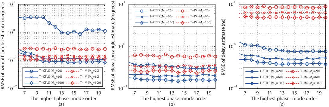
In order to validate Theorem 1, Fig. 6 plots the RMSE of the parameter estimation versus the highest order, $P$ , with different numbers of horizontal array steering vectors. The SNR is -5 dB. We see that when $P$ is less than 10 or the number of the horizontal array steering vectors in (5) is 20, the algorithms applying Theorem 1 to design the hybrid beamformers (i.e., T-CTLS and M-CTLS), cannot achieve satisfactory estimation, because the number of the transformed beamspace vectors (6) is not sufficient to represent the array response vectors. When $P\geq 12$ , regardless of the number of array response vectors, increasing the beamspace vectors has little impact on the estimation. By exploiting this property, we can reduce the number of required RF chains and, in turn, the hardware cost.

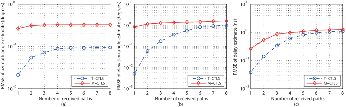
Fig. 7 shows the RMSE of the estimated azimuth angles, elevation angles, and delays, with an increasing number of received paths. T-CTLS and M-CTLS are tested. We set SNR to -5 dB and $M_{\textrm{f}}=8$ . We observe that the performance gap between the matrix and tensor forms of the proposed algorithm, i.e., M-CTLS and T-CTLS, decreases with the increasing number of received paths. This is because the noise components which can be suppressed by using the tensor-based algorithms in the first, second, and third modes of $\mathcal{Y}$ , depend on the difference between the number of paths and the tensor dimension in each mode of $\mathcal{Y}$ . As the number of received paths increases, the gain of the tensor-based algorithm, T-CTLS, diminishes. The performance gap remains consistent in Fig. 7(a) though. This is because, despite the number of paths increases, the dimension in the first mode of $\mathcal{Y}$ , i.e., $M_{\textrm{vd}}=2P+1$ , is still much larger than the number of paths. Moreover, we estimate the azimuth angles with tensor-MUSIC in (51). The method involves peak search, and is hardly affected by the number of paths. In conclusion, the new tensor-based algorithm, T-CTLS, can achieve much better performance than its matrix-based counterpart, especially under B5G settings where the number of received paths is small due to the sparsity of mmWave propagation.

VII Conclusion

We presented a new tensor-based multi-dimensional channel parameter estimation algorithm for 5G/B5G wideband mmWave large-scale hybrid antenna arrays. By exploiting the multidimensional structure of the received signals, the algorithm can suppress the noises across all domains of the received signals, improving estimation accuracy. Specifically, we designed the hybrid beamformers to maintain the angular resolution and suppress beam squinting. We developed the new HOSVD model to suppress the noise, and revealed the shift-invariance relations in the tensor form. Given the relations, we designed the new tensor-based TLS-ESPRIT algorithm for parameter estimation. We also rearranged the measurement tensor to estimate coherent signals. By applying the channel parameters presented by 3GPP TR 38.901 [31], simulations show that the proposed tensor-based algorithm can accurately estimate the multi-dimensional parameters in typically used mmWave channels, even under low SNRs.

Appendix I

Properties of Tensor Operation

The important properties of tensor operations used in this paper are provided below.

Property 1.

The $n$ -mode product satisfies the following properties:

\mathcal{A}\times_{n}\mathbf{B}\times_{n}\mathbf{C}=\mathcal{A}\times_{n}\left(\mathbf{CB}\right);

(58)

\mathcal{A}\times_{n}\mathbf{B}\times_{m}\mathbf{D}=\mathcal{A}\times_{m}\mathbf{D}\times_{n}\mathbf{B},

(59)

where $\mathcal{A}\in\mathbb{C}^{I_{1}\times I_{2}\times\cdots\times I_{N}}$ , $\mathbf{B}\in\mathbb{C}^{J_{n}\times I_{n}}$ , $\mathbf{C}\in\mathbb{C}^{K_{n}\times J_{n}}$ , and $\mathbf{D}\in\mathbb{C}^{J_{m}\times I_{m}}$ $(n,m=1,2,\ldots,N$ and $n\neq m)$ .

Property 2.

The Tucker decomposition decomposes a tensor $\mathcal{A}\in\mathbb{C}^{I_{1}\times I_{2}\times\cdots\times I_{N}}$ into a core tensor $\mathcal{G}\in\mathbb{C}^{R_{1}\times R_{2}\times\cdots\times R_{N}}$ multiplied by a factor matrix $\mathbf{C}^{(n)}=\left[\mathbf{c}_{r_{n}=1}^{(n)},\mathbf{c}_{r_{n}=2}^{(n)},\ldots,\mathbf{c}_{r_{n}=R_{n}}^{(n)}\right]\in\mathbb{C}^{I_{n}\times R_{n}}$ ( $\mathbf{c}_{r_{n}}^{(n)}\in\mathbb{C}^{I_{n}\times 1}$ and $n=1,2,\ldots,N$ ) in each mode, i.e.,

	$\displaystyle\mathcal{A}$	$\displaystyle=\sum_{r_{1}=1}^{R_{1}}\sum_{r_{2}=1}^{R_{2}}\cdots\sum_{r_{N}=1}^{R_{N}}g_{r_{1}r_{2}\cdots r_{N}}\left(\mathbf{c}_{r_{1}}^{(1)}\circ\mathbf{c}_{r_{2}}^{(2)}\circ\cdots\mathbf{c}_{r_{N}}^{(N)}\right)$
		$\displaystyle=\left\llbracket\mathcal{G};\mathbf{C}^{(1)},\mathbf{C}^{(2)},\ldots,\mathbf{C}^{(N)}\right\rrbracket.$		(60)

The HOSVD is a special case of the Tucker decomposition, where the core tensor is all-orthogonal [18], and the factor matrices are the unitary left singular matrices of the mode- $n$ unfolding of $\mathcal{A}$ .

Property 3.

The CANDECOMP/PARAFAC (CP) decomposition decomposes a tensor $\mathcal{A}\in\mathbb{C}^{I_{1}\times I_{2}\times\cdots\times I_{N}}$ into a sum of rank-one component tensors $\mathbf{b}_{r}^{(n)}\in\mathbb{C}^{I_{n}}$ , as given by

\mathcal{A}=\sum_{r=1}^{R}\lambda_{r}\mathbf{b}_{r}^{(1)}\circ\mathbf{b}_{r}^{(2)}\circ\cdots\mathbf{b}_{r}^{(N)},

(61)

where $R=\textrm{Rank}(\mathcal{A})$ is the rank of $\mathcal{A}$ ⁶⁶ 6 The rank of a tensor, $\mathcal{A},$ denoted $\textrm{Rank}(\mathcal{A})$ , is defined as the smallest number of rank-one tensors that yield $\mathcal{A}$ in a linear combination [18].. Following [18], CP can be viewed as the special case of the Tucker decomposition, where the core tensor is superdiagonal. Thus, the CP model in (61) can be rewritten as a multilinear product:

	$\displaystyle\mathcal{A}$	$\displaystyle=\mathcal{D}\times_{1}\mathbf{B}^{(1)}\times_{2}\mathbf{B}^{(2)}\cdots\times_{N}\mathbf{B}^{(N)}$
		$\displaystyle=\left\llbracket\mathcal{D};\mathbf{B}^{(1)},\mathbf{B}^{(2)},\ldots,\mathbf{B}^{(N)}\right\rrbracket,$		(62)

where $\mathbf{B}^{(n)}=\left[\mathbf{b}_{1}^{(n)},\mathbf{b}_{2}^{(n)},\ldots,\mathbf{b}_{R}^{(n)}\right]\in\mathbb{C}^{J_{n}\times R}$ is the factor matrix of $\mathbf{b}_{r}^{(n)}$ , and $\mathcal{D}\in\mathbb{C}^{R\times R\times\cdots\times R}$ is a superdiagonal tensor⁷⁷ 7 A tensor $\mathcal{A}\in\mathbb{C}^{I_{1}\times I_{2}\times\cdots\times I_{N}}$ is diagonal if $a_{i_{1}i_{2}\cdots i_{N}}\neq 0$ only if $i_{1}=i_{2}=\cdots=i_{N}$ . When $I_{1}=I_{2}=\cdots=I_{N}$ , $\mathcal{A}$ is called as superdiagonal. with $d_{r,r,\cdots,r}=\lambda_{r}$ .

Property 4.

The multilinear product of a tensor $\mathcal{A}\in\mathbb{C}^{I_{1}\times I_{2}\times\cdots\times I_{N}}$ with matrices $\mathbf{B}^{(n)}\in\mathbb{C}^{J_{n}\times I_{n}}$ , $n=1,2,\ldots,N$ , is a sequence of contractions, each being an $n$ -mode product, i.e.,

\mathcal{C}=\mathcal{A}\times_{1}\mathbf{B}^{(1)}\times_{2}\mathbf{B}^{(2)}\cdots\times_{N}\mathbf{B}^{(N)}\in\mathbb{C}^{J_{1}\times J_{2}\times\cdots\times J_{N}}.

(63)

Its mode- $n$ unfolding is given by

	$\displaystyle\mathbf{C}_{(n)}$	$\displaystyle=\mathbf{B}^{(n)}\mathbf{A}_{(n)}(\mathbf{B}^{(n+1)}\otimes\mathbf{B}^{(n+2)}\otimes$
		$\displaystyle\cdots\otimes\mathbf{B}^{(N)}\otimes\mathbf{B}^{(1)}\otimes\mathbf{B}^{(2)}\otimes\cdots\otimes\mathbf{B}^{(n-1)})^{T}.$		(64)

Appendix II

Proof of Theorem 1

Let $\gamma_{m_{\textrm{f}}}(\theta_{k_{m_{\textrm{b}}}})=\frac{2\pi}{c}f_{m_{\textrm{f}}}r\sin(\theta_{k_{m_{\textrm{b}}}}).$ The Q-DFT of $a_{\textrm{h},m_{\textrm{f}},m_{\textrm{b}}}(\theta_{k_{m_{\textrm{b}}}},\phi_{k_{m_{\textrm{b}}}})$ can be expressed as

		$\displaystyle a_{\textrm{QDFT},p,m_{\textrm{f}},m_{\textrm{b}}}(\theta_{k_{m_{\textrm{b}}}},\phi_{k_{m_{\textrm{b}}}})$
		$\displaystyle\stackrel{{\scriptstyle(\textrm{a})}}{{=}}\sum_{m_{\textrm{h}}=1}^{M_{\textrm{h}}}\left(\frac{1}{\sqrt{M_{\textrm{h}}}}\sum_{q=-\infty}^{\infty}j^{q}J_{q}(\gamma_{m_{\textrm{f}}}(\theta_{k_{m_{\textrm{b}}}}))e^{jq(\phi_{k_{m_{\textrm{b}}}}-\varphi_{m_{\textrm{h}}})}\right)$
		$\displaystyle\qquad\qquad\times e^{-j\frac{2\pi(m_{\textrm{h}}-1)}{M_{\textrm{h}}}p}$
		$\displaystyle\stackrel{{\scriptstyle(\textrm{b})}}{{=}}\frac{1}{\sqrt{M_{\textrm{h}}}}\sum_{Q=-\infty}^{\infty}M_{\textrm{h}}j^{(QM_{\textrm{h}}-p)}J_{(QM_{\textrm{h}}-p)}(\gamma_{m_{\textrm{f}}}(\theta_{k_{m_{\textrm{b}}}}))$
		$\displaystyle\qquad\qquad\times e^{j(QM_{\textrm{h}}-p)\phi_{k_{m_{\textrm{b}}}}}$
		$\displaystyle\stackrel{{\scriptstyle(\textrm{c})}}{{=}}\sqrt{M_{\textrm{h}}}[j^{p}J_{p}(\gamma_{m_{\textrm{f}}}(\theta_{k_{m_{\textrm{b}}}}))e^{-jp\phi_{k_{m_{\textrm{b}}}}}$
		$\displaystyle+\sum_{Q=-\infty,Q\neq 0}^{\infty}\varepsilon_{p,Q}(\gamma_{m_{\textrm{f}}}(\theta_{k_{m_{\textrm{b}}}}),\phi_{k_{m_{\textrm{b}}}})]$		(65)

where

		$\displaystyle\varepsilon_{p,Q}(\gamma_{m_{\textrm{f}}}(\theta_{k_{m_{\textrm{b}}}}),\phi_{k_{m_{\textrm{b}}}})$
		$\displaystyle=j^{(QM_{\textrm{h}}-p)}J_{(QM_{\textrm{h}}-p)}(\gamma_{m_{\textrm{f}}}(\theta_{k_{m_{\textrm{b}}}}))e^{j(QM_{\textrm{h}}-p)\phi_{k_{m_{\textrm{b}}}}}.$		(66)

In (65), $(\textrm{a})$ and $(\textrm{c})$ follow the important properties of the Bessel function, i.e., $e^{jx\cos y}=\sum_{v=-\infty}^{\infty}j^{v}J_{v}(x)e^{jvy}$ and $J_{-v}(x)=(-1)^{v}J_{v}(x)$ , respectively; $(\textrm{b})$ is obtained by letting $p+q=QM_{\textrm{h}}$ ; and $(\textrm{c})$ stems from the property of the Bessel function $J_{-v}(x)=(-1)^{v}J_{v}(x)$ [34].

Consider that the number of antennas per UCA, $M_{\textrm{h}}$ , is large, i.e, $M_{\textrm{h}}\gg P$ . Let $M_{\textrm{h}}=\alpha P$ and $\gamma_{m_{\textrm{f}}}(\theta_{k_{m_{\textrm{b}}}})=\beta P,$ where $\alpha\gg 1$ and $0<\beta<1$ . According to [34], we have $J_{v}(v\rho)<J_{v}(v)$ and $J_{v_{1}}(v_{1}\rho)<J_{v_{2}}(v_{2}\rho)$ , where $v_{1}>v_{2}$ and $\rho\in(0,1)$ . Since $P\geq\left\lfloor 2\pi f_{m_{\textrm{f}}}r/c\right\rfloor$ , we have $J_{(QM_{\textrm{h}}-p)}(\gamma_{m_{\textrm{f}}}(\theta_{k_{m_{\textrm{b}}}}))<J_{(\alpha-1)P}\left(\beta P\right)$ and $J_{P}\left(\beta P\right)\leq J_{p}(\gamma_{m_{\textrm{f}}}(\theta_{k_{m_{\textrm{b}}}}))$ . Set $\alpha=3$ and $\beta=0.5$ for an example. In general, $P>3$ . Hence, $J_{p}(\gamma_{m_{\textrm{f}}}(\theta_{k_{m_{\textrm{b}}}}))\geq J_{3}\left(1.5\right)\approx 0.06$ and

		$\displaystyle J_{(Q_{2}M_{\textrm{h}}-p)}(\gamma_{m_{\textrm{f}}}(\theta_{k_{m_{\textrm{b}}}}))<J_{(Q_{1}M_{\textrm{h}}-p)}(\gamma_{m_{\textrm{f}}}(\theta_{k_{m_{\textrm{b}}}}))$
		$\displaystyle<J_{(M_{\textrm{h}}-p)}(\gamma_{m_{\textrm{f}}}(\theta_{k_{m_{\textrm{b}}}}))<J_{6}\left(1.5\right)\approx 0.0002,$		(67)

where $Q_{2}>Q_{1}>1$ . Compared with $J_{p}(\gamma_{m_{\textrm{f}}}(\theta_{k_{m_{\textrm{b}}}}))$ , the amplitude of $J_{(QM_{\textrm{h}}-p)}(\gamma_{m_{\textrm{f}}}(\theta_{k_{m_{\textrm{b}}}}))$ is so small and can be omitted. We suppress $\varepsilon_{p,Q}(\gamma_{m_{\textrm{f}}}(\theta_{k_{m_{\textrm{b}}}}),\phi_{k_{m_{\textrm{b}}}})$ and approximate (65) as

		$\displaystyle a_{\textrm{QDFT},p,m_{\textrm{f}},m_{\textrm{b}}}(\theta_{k_{m_{\textrm{b}}}},\phi_{k_{m_{\textrm{b}}}})$
		$\displaystyle\approx\sqrt{M_{\textrm{h}}}j^{p}J_{p}(\gamma_{m_{\textrm{f}}}(\theta_{k_{m_{\textrm{b}}}}))\exp(-jp\phi_{k_{m_{\textrm{b}}}}).$		(68)

This concludes the proof of Theorem 1.

References

[1] A. Shahmansoori, G. E. Garcia, G. Destino, et al., “Position and orientation estimation through millimeter-wave MIMO in 5G systems,” IEEE Trans. Wireless Comm., vol. 17, no. 3, pp. 1822–1835, Mar. 2018.
[2] L. Zhu and J. Zhu, “Optimal design of uniform circular antenna array in mmWave LOS MIMO channel,” IEEE Access, vol. 6, pp. 61022–61029, Sep. 2018.
[3] F. E. D. Raimondi, R. C. Farias, O. J. Michel, et al., “Wideband multiple diversity tensor array processing,” IEEE Trans. Signal Process., vol. 65, no. 20, pp. 5334–5346, Oct. 2017.
[4] R. W. Heath Jr., N. G. Prelcic, S. Rangan, et al., “An overview of signal processing techniques for millimeter wave MIMO systems,” IEEE J. Sel. Topics Signal Process., vol. 10, no. 3, pp. 436–453, Apr. 2016.
[5] F. Raimondi, P. Comon, and O. Michel, “Wideband multilinear array processing through tensor decomposition,” in Proc. IEEE Int. Conf. Acoust. Speech Signal Process. (ICASSP), Shanghai, China, Mar. 2016, pp. 2951–2955.
[6] Tamara G. Kolda and Brett W. Bader, “Tensor decompositions and applications,” SIAM Rev., vol. 51, no. 3, pp. 455–500, Sep. 2009.
[7] M. Haardt, F. Roemer, and G. Del Galdo, “Higher-order SVD-based subspace estimation to improve the parameter estimation accuracy in multidimensional harmonic retrieval problems,” IEEE Trans. Signal Process., vol. 56, no. 7, pp. 3198–3213, Jul. 2008.
[8] X. Guo, Q. Wan, X. Shen, et al., “Low-complexity parameters estimator for multiple 2D domain incoherently distributed sources,” Turk. J. Elect. Eng. Comput. Sci., vol. 3, no. 19, pp. 445–462, May 2011.
[9] A. Hu, T. Lv, H. Gao, et al., “An ESPRIT-based approach for 2-D localization of incoherently distributed sources in massive MIMO systems,” IEEE J. Sel. Topics Signal Process., vol. 8, no. 5, pp. 996–1011, Oct. 2014.
[10] J. H. Brady and A. M. Sayeed, “Wideband communication with high-dimensional arrays: New results and transceiver architectures,” in Proc. IEEE Int. Conf. Commun. Workshop (ICCW), London, U.K., Jun. 2015, pp. 1042–1047.
[11] F. Sellone, “Robust auto-focusing wideband DOA estimation,” Signal Process., vol. 86, no. 1, pp. 17–37, Jan. 2006.
[12] Z. Lin, T. Lv, J. A. Zhang, et al., “3D wideband mmWave localization for 5G massive MIMO systems,” in Proc. IEEE Int. Global Commun. (GLOBECOM), Waikoloa, HI, USA, Dec. 2019, pp. 1–7.
[13] Z. Lin, T. Lv, and P. T. Mathiopoulos, “3-D indoor positioning for millimeter-Wave massive MIMO systems,” IEEE Trans. Commun., vol. 66, no. 6, pp. 2472–2486, June 2018.
[14] B. D. Van Veen and K. M. Buckley, “Beamforming: A versatile approach to spatial filtering,” IEEE Acoust. Speech Sig. Proc. Mag., vol. 5, no. 5, pp. 4–24, Apr. 1988.
[15] H. Wang and M. Kaveh, “Coherent signal-subspace processing for the detection and estimation of angles of arrival of multiple wide-band sources,” IEEE Trans. Acoust. Speech Signal Process., vol. 33, no. 4, pp. 823–831, Aug. 1985.
[16] G. Bienvenu, P. Fuerxer, G. Vezzosi, L. Kopp, and F. Florin, “Coherent wide band high resolution processing for linear array,” in Proc. IEEE Int. Conf. Acoust. Speech Signal Process. (ICASSP), May 1989, vol. 4, pp. 2799–2802.
[17] M. Wang, F. Gao, N. Shlezinger, et al., “A block sparsity based estimator for mmWave massive MIMO channels with beam squint,” IEEE Trans. Signal Process., vol. 68, pp. 49–64, Sep. 2020.
[18] L. D. Lathauwer, B. D. Moor, and J. Vandewalle, “A multilinear singular value decomposition,” SIAM J. Matrix Anal. Appl., vol. 21, no. 4, pp. 1253–1278, Mar. 2000.
[19] A. Cichocki, D. Mandic, L. De Lathauwer, et al., “Tensor decompositions for signal processing applications: From two-way to multiway component analysis,” IEEE Signal Process., vol. 32, no. 2, pp. 145–163, Mar. 2015.
[20] P. Forster, G. Ginolhac, and M. Boizarda, “Derivation of the theoretical performance of a tensor MUSIC algorithm,” Signal Process., vol. 129, pp. 97–105, Dec. 2016.
[21] J. Steinwandt, F. Roemer, and M. Haardt, “Performance analysis of ESPRIT-type algorithms for non-circular sources,” in Proc. IEEE Int. Conf. Acoust. Speech Signal Process. (ICASSP), May 2013, pp. 3986–3990.
[22] Z. Lin, T. Lv, J. A. Zhang, et al., “Tensor-based high-accuracy position estimation for 5G mmWave massive MIMO systems,” in Proc. IEEE Int. Conf. Commun. (ICC), Dublin, Ireland, Jun. 2020, pp. 1–7.
[23] Z. Zhou, J. Fang, L. Yang, et al., “Low-rank tensor decomposition-aided channel estimation for millimeter wave MIMO-OFDM systems,” IEEE J. Sel. Areas Commun., vol. 35, no. 7, pp. 1524–1538, July 2017.
[24] F. Wen, N. Garcia, J. Kulmer, K. Witrisal, and H. Wymeersch, “Tensor decomposition based beamspace ESPRIT for millimeter wave MIMO channel estimation,” in Proc. IEEE Int. Global Commun. (GLOBECOM), Dec. 2018, pp. 1–7.
[25] S. Jeong, X. Li, J. Yang, et al., “Sparse representation-based denoising for high-resolution brain activation and functional connectivity modeling: A task fMRI study,” IEEE Access, vol. 8, pp. 36728–36740, Feb. 2020.
[26] R. J. Mailloux, Phased Array Antenna Handbook, Artech House, Norwood, United States, 2nd edition, 2005.
[27] D. H. Johnson and D. E. Dudgeon, Array Signal Processing: Concepts and Techniques, NJ: Prentice-Hall, Englewood Cliffs, USA, 1993.
[28] M. C. Vanderveen, A. J. van der Veen, and A. Paulraj, “Estimation of multipath parameters in wireless communications,” IEEE Trans. Signal Process., vol. 46, no. 3, pp. 682–690, Mar. 1998.
[29] K. Abed-Meraim and Y. Hua, “A least-squares approach to joint schur decomposition,” in Proc. IEEE Int. Conf. Acoust. Speech Signal Process. (ICASSP), May 1998, vol. 4, pp. 2541–2544.
[30] F. Roemer, M. Haardt, and G. Del Galdo, “Analytical performance assessment of multi-dimensional matrix- and tensor-based ESPRIT-type algorithms,” IEEE Trans. Signal Process., vol. 62, no. 10, pp. 2611–2625, May 2014.
[31] 3GPP TR 38.901 V14.1.1, “Study on channel model for frequencies from 0.5 to 100 GHz (rel. 14),” Jul. 2017.
[32] A. Guerra, F. Guidi, and D. Dardari, “Position and orientation error bound for wideband massive antenna arrays,” in Proc. IEEE Int. Conf. Commun. Workshop (ICCW), London, UK, Jun. 2015, pp. 1–6.
[33] D. Wang, M. Fattouche, and X. Zhan, “Pursuance of mm-level accuracy: Ranging and positioning in mmWave systems,” IEEE Systems J., vol. PP, no. 99, pp. 1–12, Mar. 2018.
[34] G. N. Watson, A Treatise on the Theory of Bessel Functions, Cambridge Univ. Press, Cambridge, U.K., 2nd edition, 1952.

$\displaystyle\hat{\mathbf{\Upsilon}}_{\textrm{v}}$	$\displaystyle=\arg\min_{\mathbf{\Upsilon}_{\textrm{v}}}\left\\|\mathbf{\Upsilon}_{\textrm{v}1}\mathbf{U}_{\textrm{s}}{}_{(4)}\left(\mathbf{J}_{\textrm{v}1}\otimes\mathbf{I}_{M_{\textrm{hd}}}\otimes\mathbf{I}_{M_{\textrm{f}}}\right)^{T}\right.$
	$\displaystyle\left.+\mathbf{\Upsilon}_{\textrm{v2}}\mathbf{U}_{\textrm{s}}{}_{(4)}\left(\mathbf{J}_{\textrm{v}2}\otimes\mathbf{I}_{M_{\textrm{hd}}}\otimes\mathbf{I}_{M_{\textrm{f}}}\right)^{T}\right\\|_{\textrm{F}}$
	$\displaystyle=\arg\min_{\mathbf{\Upsilon}_{\textrm{v}}}\left\\|\mathbf{W}_{\textrm{v}}\mathbf{\Upsilon}_{\textrm{v}}^{T}\right\\|_{\textrm{F}},$	(43)