Thermostatistical analysis for short-range interaction Potentials

M. J. Neves Note: E-mail: mneves@ufrrj.br Address: Department of Physics and Astronomy, University of Alabama, Tuscaloosa, Alabama 35487, USA;
Departamento de Física, Universidade Federal Rural do Rio de Janeiro, BR 465-07, 23890-971, Seropédica, RJ, Brazil Everton M. C. Abreu Note: E-mail: evertonabreu@ufrrj.br Address: Departamento de Física, Universidade Federal Rural do Rio de Janeiro, BR 465-07, 23890-971, Seropédica, RJ, Brazil;
Departamento de Física, Universidade Federal de Juiz de Fora, 36036-330, Juiz de Fora, MG, Brazil and
Programa de Pós-Graduação Interdisciplinar em Física Aplicada, Instituto de Física, Universidade Federal do Rio de Janeiro, 21941-972, Rio de Janeiro, RJ, Brazil Jorge B. de Oliveira Note: E-mail: jorgebernardo998@gmail.com Address: Departamento de Física, Universidade Federal Rural do Rio de Janeiro, BR 465-07, 23890-971, Seropédica, RJ, Brazil Marcelo Kesseles Gonçalves Note: E-mail: marcelokesseles@ufrrj.br Address: CAPES-PIBID/Física, Departamento de Física, Universidade Federal Rural do Rio de Janeiro, BR 465-07, 23890-971, Seropédica, RJ, Brazil

Abstract

In this paper, we study the thermodynamics of short-range central potentials, namely, the Lee-Wick potential, and the Plasma potential. In the first part of the paper we obtain the numerical solution for the orbits equation for these potentials. Posteriorly, we introduce the thermodynamics through the microcanonical and canonical ensembles formalism defined on the phase space of the system. We calculate the density of states associated with the Lee-Wick and the Plasma potentials. From density of states, we obtain the thermodynamical physical quantities like entropy and temperature as functions of the energy. We also use the Boltzmann-Gibbs formalism to obtain the partition functions, the mean energy and the thermal capacity for these short-range potentials.

keywords

Lee-Wick Potential; Debye-Hückel potential; thermodynamics of central potentials; Boltzmann-Gibbs statistics

^†^†catchline: Vol. , No. () –^†^†history: Received (09 August 2020)Revised (03 September 2020)

1 Introduction

The Yukawa Potential (YP) in atomic physics, namely, the Debye-Hückel potential in plasma physics, is also known as the screened Coulomb potential and it deserves the interest of researches of many areas of physics [1, 2]. It has its origins in the intention of describing, in a much more precise way, the interactions of forces that act at very small distances.

Originally, we can describe the interactions, for example, of the strong force inside atomic nucleus, i.e., the strong nucleons-nucleons interactions, thanks to the meson exchange, depicted in nuclear physics. Concerning the Coulomb potential having the $K/r$ formulation, where $K$ is any constant, it is good to describe the general force effects, where the limit of the interaction has an almost infinite limit. We know that if any charge is a very small one, we have a bigger potential and, if the distance is big, we have a small potential. However, the same is not true to evaluate the strong force, since it is measured only at very small distances, which has a very small interaction limit. To work with these limitations is why H. Yukawa investigated and developed the potential that, today, has his name [1, 2].

As we said just above, the YP can also be used to show a screened Coulomb potential due to the cloud of electronic charges around the nucleus in atomic physics. Or to represent the shielding by outer charges of the Coulomb field that an atomic electron feels in hydrogen plasma. Although the Schrödinger equation concerning this potential cannot be solved exactly, there are various numerical and perturbation methods that have been thought up in order to capture the energy levels and related physical quantities [3].

It is very clear to theoretical physicists that there is a connection between the field equations of gravity and the first law of thermodynamics on the boundary of spacetime [4, 5, 6]. This correspondence leads us to the entanglement between thermodynamics and gravitation, which has been explored since the work of Jacobson [4]. Recently, the proposal of Verlinde [7] conjectures that gravity is an emergent phenomenon due to the increasing of entropy. This emergence occurs between holographic screens [8], which is a fundamental ingredient together with entropy. Its importance can be seen through several corrections to the entropic-area expression, which introduces several modifications into gravity theories and their respective cosmology [9, 10]. Since it was demonstrated [10] that, if the Unruh temperature [11] is connected to the holographic screen, so the quantum statistics of the surface degrees of freedom can help us to obtain a theoretical cornerstone concerning the well known Modified Newtonian Dynamics (MOND) theory [12].

To explain the accelerated expansion of the Universe, thermodynamical pictures have been described. One of them is the Bekenstein-Hawking entropy, where this last one is proportional to the surface area of the event horizon [13, 14]. The other important scenario is the holographic principle (HP), in which the information of the bulk is stored on the horizon [15]. The HP was used to propose that gravity is an entropic force obtained from changes in Bekenstein-Hawking entropy [4, 7, 5]. To demonstrate this concept, the cosmological equations have been widely investigated in an homogeneous and isotropic Universe [16]. However, the cosmological constant was not discussed. Alternatively, in [17] the author suggested an entropic cosmology that takes into account the neglected surface terms on the horizon of the Universe [18, 19, 20, 21, 22, 23]. In this so-called entropic cosmology, the explanation of the accelerated expansion was obtained from the entropic forces on the horizon of the Universe.

Thermodynamical analysis were carried out for different potential in the last few years. In [24], the authors analyzed the thermodynamics of the Schroedinger equation with a Deng-Fan-type potential. In [25], it was studied the Klein-Gordon approach or particles embedded in exponential-type molecule potential together with their thermodynamical characteristics in $D$ dimensions. The harmonic oscillator plus an inverse square potential were investigated thermodynamically in [26]. Concerning different diatomic molecules, their thermodynamical properties were analyzed in [27, 28] and with general molecular potential in [29]. In [30], the authors solved the Schroedinger equation using the modified factorization method for the modified Yukawa potential, also known as generalized inversely quadratic Yukawa potential. Hence, we can see the importance of the thermodynamics analysis in any kind of interaction.

In this work we have analyzed the thermodynamical aspects of several different short-range potentials, The microcanonical and canonical formalisms were carried out and compared. Thermodynamical and statistical mechanics quantities like entropy, temperature were computed together with the partition function, mean energy and heat capacity, respectively.

We have organized the discussion of these issues in such a way that in section 2 where we have described some classical aspects of short-range potentials such as force and equations of motion. In section 3 we analyzed the thermodynamical aspects of these short-range potentials and in section 4, their statistical mechanics results. In section 5, we made some discussions, conclusions and perspectives.

2 The orbit equation for short-range forces

Differently from the Coulomb potential, the Lee-Wick (LW) [33, 34, 35] short-range potential shows an association with the involved particles’ masses. In other words, LW realized that the interactions, in general, are inversely proportional to the potential mediator’s mass. In this way, he has developed a potential that has the following form¹¹ 1 We are considering the natural units $\hbar=c=1$ .:

\displaystyle V_{LW}(r)=K\,\frac{1-e^{-\mu\,r}}{r}\;,

(1)

where $K$ is the potential strength and $\mu=Mm/(M+m)$ represents the reduced mass between the two particles masses, $M$ and $m$ . Note that the LW potential is the subtraction of the Coulomb with the Yukawa potential. Furthermore, when $\mu r\ll 1$ , the potential function is finite at the origin, and its value is $V_{LW}(r=0)=K\mu$ .

We can see clearly that the potential is monotone increasing in $r$ and after a certain point, it turns to be negative, which means that the force goes to be attractive. It is worth mentioning that, relative to the interactions between both a meson field and a fermion field, the constant $K$ has the same value as the gauge coupling constant between both fields.

Concerning the Coulomb potential case, the reduced mass goes to zero, which represents a zero mass boson as being the potential mediator, and $K$ can have positive or negative real values. Specifically, for $K>0$ it has been found in the literature that the S-wave bound states exist only for values of $\mu$ below just a determined critical value $\mu_{c}\sim 1.1906\,A$ in atomic units [39]. Moreover, differently from the Coulomb potential, the Yukawa one permits the appearance of resonant states. Questions about the solution of the Schrödinger equation for this potential were investigated intensely in the past by using several numerical and perturbative analyzes. The reason is that it is not possible to find exact analytical solutions since there is a lack of shape invariance relative to this potential [42]. Considering the short-range behavior of the YP due to the decaying exponential term (i.e., $e^{-\mu r}$ ), there is a singularity at the origin thanks to $r^{-1}$ . The centrifugal term $r^{-2}$ behavior, together with the exponential term, both are responsible for the non-trivial task of obtaining accurate numerical solutions. To provide a thermodynamical investigation, in this work we will analyze the short-range interaction problem using, among others, the YP.

2.1 The central potential: a quick review

Since a central force $F(r)$ is conservative, it can be written as minus the radial derivative of a $U(r)$ potential function. The motion of two particles of masses $M$ and $m$ , that interact under the action of central force $F(r)$ , is described by the radial equation

\displaystyle\mu\,\ddot{r}=-\frac{dU_{eff}}{dr}\;,

(2)

where $r$ is the relative coordinate between $M$ and $m$ , $U_{eff}(r)$ is the effective potential that can be written as

\displaystyle U_{eff}(r)=U(r)+\frac{L^{2}}{2\mu r^{2}}\;,

(3)

where the quantity $L^{2}$ means the conserved angular momentum of a general two-particle system. Since we know the form of the potential function $U(r)$ , the equation of motion in Eq. (2) can be integrated to obtain the radial solution as a function of time. In the case of an interaction force system, it is well known that the trajectory carried out by $m$ interacting with $M$ is given by

\displaystyle\frac{d^{2}r}{d\theta^{2}}-\frac{2}{r}\left(\frac{dr}{d\theta}\right)^{2}=r+\left(\frac{\mu r^{4}}{L^{2}}\right)F(r)\;.

(4)

To solve the previous equation in order to ease the calculations, we will provide a variable transformation of the kind $u=1/r$ . In this way, the final form of the equations of motion is

\displaystyle\frac{d^{2}u}{d\theta^{2}}+u=-\frac{\mu}{L^{2}u^{2}}\,F\left(\frac{1}{u}\right)\;.

(5)

Therefore, if we know the form of both functions $U(r)$ and $F(r)$ , we can determine the information about the behavior of $m,\,M$ and its corresponding trajectory. We will use several potentials in the next subsections.

2.2 The orbit solution for the Lee-Wick potential

To analyze the kind of interaction that comes from the Lee-Wick (LW) potential, we can say that the force generated by it is, considering the work and energy theorem, a central force. We can say the same concerning all the potentials that will be considered here. Having said that, we can use the relation between force and potential energy. Considering the LW case in Eq. (1), the corresponding effective potential is given by

\displaystyle V_{eff}^{(LW)}(r)=-|K|\,\frac{1-e^{-\mu\,r}}{r}+\frac{L^{2}}{2\mu r^{2}}\,\,,

(6)

and its behavior is shown in figure (1).

Refer to caption — Figure 1: Left panel: Plot of Lee-Wick potential by $\mu|K|$ units versus the dimensionless $\mu r$ . Right panel: The Lee-Wick effective potential as function of the radial distance.

If we analyze the effective potential energy of the system, under the same conditions used before, we could obtain the points of maximum distance and maximum proximity, since we consider that at these points it does not exist kinetic energy. Hence, from

\displaystyle V_{eff}^{(LW)}(r)\simeq\frac{L^{2}}{2\mu r^{2}}+\frac{K}{r}-\mu\,K\;,

(7)

where these distances are obtained by making $V_{eff}^{LW}(r)=-|E|$ , where we can consider as negative the total energy of system. If we make the necessary calculations, we have that

\displaystyle\frac{1}{r_{\pm}}=\frac{\mu\,|K|}{L^{2}}\,\pm\sqrt{\frac{\mu^{2}|K|^{2}}{L^{4}}-\frac{2\mu}{L^{2}}\left(|E|+\mu|K|\right)}\,\,,

(8)

and the turning points are

	$\displaystyle\frac{1}{r_{p}}$	$\displaystyle=$	$\displaystyle\frac{\mu\,\|K\|}{L^{2}}\left(1\,+\,\sqrt{1\,-\,\frac{2\,L^{2}}{\mu\,\|K\|^{2}}(\|E\|+\mu\|K\|)}\,\right)\;,$		(9)
	$\displaystyle\frac{1}{r_{a}}$	$\displaystyle=$	$\displaystyle\frac{\mu\,\|K\|}{L^{2}}\left(1\,-\,\sqrt{1\,-\,\frac{2\,L^{2}}{\mu\,\|K\|^{2}}(\|E\|+\mu\|K\|)}\right)\;,$		(10)

where $r_{p}$ is the point of maximum approximation, and $r_{a}$ is the point of maximum distance. Namely, considering the point $r_{p}$ , we have the smaller distance between $M$ and $m$ and and the point $r_{a}$ is just the opposite, where they will be at a maximum distance, i.e., they still interact, and after that point, they will not.

The radial interaction force generated by the LW potential is given by

\displaystyle F_{LW}(r)=-\frac{K}{r^{2}}+\frac{K}{r^{2}}\,e^{-\mu r}\,\left(\,1+\mu\,r\,\right)\;,

(11)

where, if we consider $K>0$ , we have that $F(r)>0$ , which characterizes a repulsive force. On the other hand, if the $K$ value is negative, the value of $F_{LW}(r)$ will be negative, which characterizes an attractive force.

As we said before, the Yukawa potential was created to describe the very small distance (short-range) interactions, i. e., $\mu r\ll 1$ . Hence, considering the limit of the interaction force as being

\displaystyle F_{LW}(r)\simeq-\frac{|K|}{r^{2}}+\frac{|K|}{r^{2}}\left(1\,-\,\mu^{2}r^{2}\right)\simeq-\mu^{2}|K|\;,

(12)

and by solving this limit, we obtain that, for distances that have a tendency of being very small. The interaction force tends to have a very strong interaction such that this type of force, when $r\rightarrow 0$ , increases as the bodies are closer. Moreover, if $r\rightarrow\infty$ we can verify that the interaction force goes to zero, since it has a negative exponential function.

To use the interaction force of the LW potential we have, firstly, to change the same variable $r$ and we will have a new variable $u$ such that $u\,=\,1/r$ . Hence, the orbit equation will be constructed as

\displaystyle\frac{d^{2}u}{d\theta^{2}}+u=-\frac{\mu K}{L^{2}}\,\left[-1+\left(1+\frac{\mu}{u}\right)e^{-\frac{\mu}{u}}\right]\;.

(13)

Since the LW potential works only in the nuclear scale, $r\rightarrow 0$ , we will adopt an approximation such that $\mu r\ll 1$ and the reduced mass, at the nuclear level is very small, just like the distance between them. In this case, the orbit equation turns out to be a non-linear differential equation given by

\displaystyle\frac{d^{2}u}{d\theta^{2}}+u\simeq\frac{\mu^{3}\,K}{L^{2}\,u^{2}}\;.

(14)

For this second order differential equation, the analytical solution has the form

u(\theta)\,=-\frac{\mu\,K}{L^{2}}+A\,\cos\left(\theta-\theta_{0}\right)-\frac{\mu^{3}\,K}{L^{2}}\left[\,\cos(\theta)\,\mbox{cosintegral}(\theta)+\mbox{sen}(\theta)\,\mbox{senintegral}(\theta)\,\right]\;,

(15)

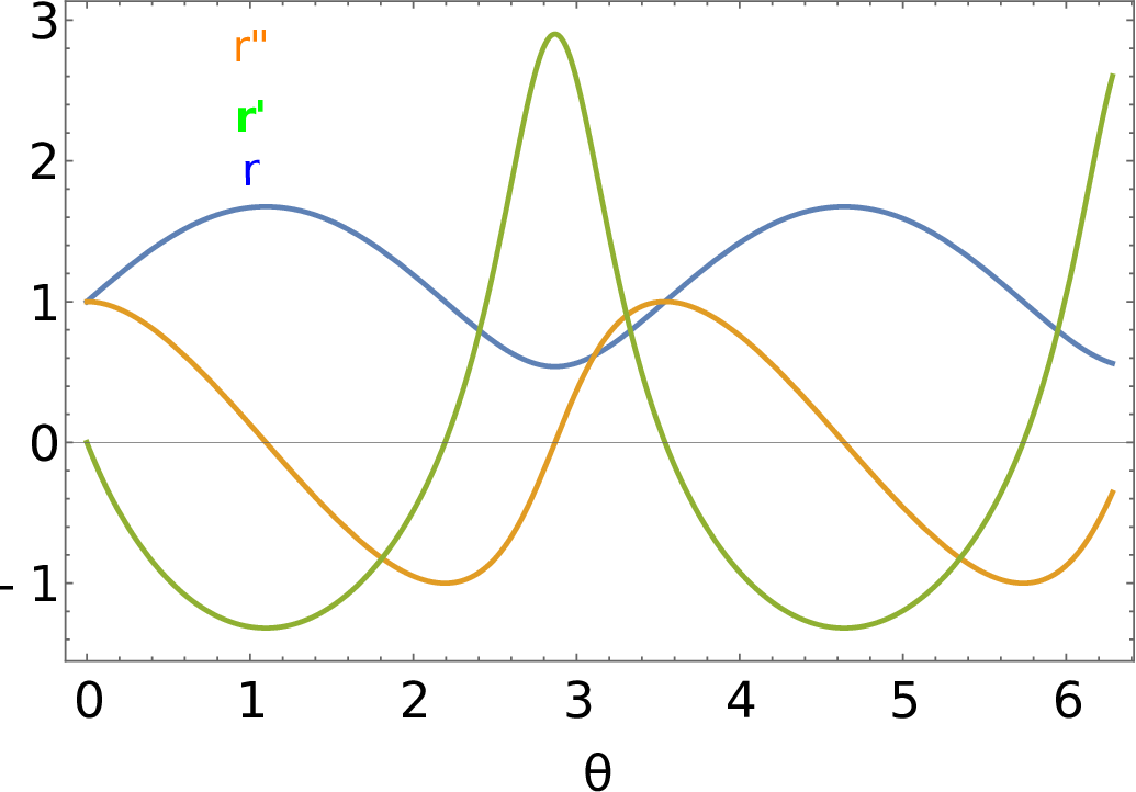
and this solution, using a ( $r-\theta$ ) plane, is shown (blue line) in figure (2). In the same figure, the first derivative $r^{\prime}$ (green line) and the second one $r^{\prime\,\prime}$ (orange line) are also shown as a function of the $\theta$ -angle.

2.3 The orbit solution for Debye-Hückel potential

The Debye-Hückel potential, known in plasma physics, can be represented by the central potential

\displaystyle V_{DH}(r)=-V_{o}\,\Big(1\,-\,\frac{a}{r}\,e^{-\alpha r}\Big)^{2}=-\,\frac{A}{r^{2}}\,e^{-2\alpha r}\,+\,\frac{B}{r}\,e^{-\alpha r}\,-\,C\;,

(16)

where $a$ is a constant carrying the length dimension, $A=a^{2}\,V_{o}$ , $B=2\,a\,V_{o}$ and $C=V_{o}$ , $V_{o}$ is the coupling strength and $\alpha$ is the potential screening parameter with length dimension. The effective potential associated with the one in Eq. (16) is shown in figure (4). The value of the parameters $A,\,B$ and $C$ can represent several potentials. For example, if $A=C=0$ and $B\,\rightarrow\,-B/2$ , we have the standard Yukawa potential. For $\alpha=0$ we have the Mie-type potential. For $B=C=0$ and $A=-V_{o}$ , the inversely quadratic Yukawa potential. And for $A=C=0$ and $\alpha=0$ , the Coulomb potential.

The Mie potential was suggested by Gustav Mie in 1903 [36]. It deals with intermolecular pair potential between two particles at a distance $r$ . It is a very used approximation concerning $n$ -body interactions.

The modified Yukawa potential is asymptotic to a finite value as $r\rightarrow 0$ and turns out to be infinite at $r=0$ [37]. Its application in many areas of physics was investigated recently [38]. The Yukawa potential can be used in plasma physics, i.e., the so-called Debye-Hückel potential. In solid state physics and atomic physics, it is known as the Thomas-Fermi or screened Coulomb potential. In nuclear physics, it is the dominant central part of nucleon-nucleon interaction.

The central force associated with the potential in Eq. (16) is given by

\displaystyle F_{DH}(r)=-\frac{2\,a\,V_{o}}{r^{2}}\,e^{-\alpha r}\left(1+\alpha r\right)\left(1+\frac{a^{2}\,e^{-\alpha r}}{r}\right)\;,

(17)

where the equation of motion for this central force can be written as

\displaystyle\frac{d^{2}u}{d\theta^{2}}+u=\frac{2\,\mu\,a\,V_{o}}{L^{2}\,u}\,e^{-\alpha/u}\left(\,1+\frac{\alpha}{u}\,\right)\left(\,1+a^{2}\,u\,\,e^{-\alpha/u}\,\right)\;.

(18)

Note that, for large distances, $\alpha r\gg 1$ , the force in Eq. (17) goes to zero. But for very short distance $\alpha r\ll 1$ , we obtain the approximated result

\displaystyle F_{DH}(r)\simeq\frac{2\,K}{\alpha^{2}\,r^{3}}\;,

(19)

and the equation of motion in Eq. (18) can be reduced to standard differential equation

\displaystyle\frac{d^{2}u}{d\theta^{2}}+a^{2}\,u\simeq 0\;,

(20)

where $a=\sqrt{1+2\,\mu\,V_{o}/(\alpha L)^{2}}$ . The solution of Eq. (20) is well known and it is given by

u(\theta)\simeq A\,\cos\left[\,a\,\left(\theta-\theta_{0}\right)\,\right]\;.

(21)

For the Mie potential, the force is given by

F(u)\,=\,-\,2\,a\,V_{o}\,u^{2}\,\Big(1\,+\,a^{2}\,u\Big)\;,

(22)

and the dynamical equation is

\frac{d^{2}u}{d\theta^{2}}+u=\frac{2a\,\mu\,V_{o}}{L^{2}}\,\Big(1\,+\,a^{2}u\Big)\,\,.

(23)

Considering the Yukawa potential,

F(u)\,=\,a\,V_{o}\,u^{3}\,e^{-\alpha/u}\,\Big(1\,+\,\frac{\alpha}{u}\Big)\,\,,

(24)

and

\frac{d^{2}u}{d\theta^{2}}+u=-\,\frac{aV_{o}u}{L^{2}}e^{-\alpha/u}\Big(1\,+\,\frac{\alpha}{u}\Big)\,\,.

(25)

Finally, for the inverse quadratic Yukawa potential

F(u)\,=\,-\,u^{3}\,e^{-\alpha/u}\Big(1\,+\,\frac{\alpha}{u}\Big)\,\,,

(26)

and

\frac{d^{2}u}{d\theta^{2}}+u=\frac{\mu u}{L^{2}}\,e^{-\alpha/u}\,\Big(1\,+\,\frac{\alpha}{u}\Big)\,\,.

(27)

After these classical results we could ask what would be their behaviors if we intend to introduce quantum features into these potentials. Or a semi-classical analysis would be more physically profitable. One way to introduce this semi-classical features is through the analysis of the behavior of these potentials in noncommutative phase-spaces. It is an ongoing research which will published elsewhere.

From now on we will investigate the thermostatistical features of the potential discussed above. We will use both the microcanonical and canonical ensemble formalisms.

3 Thermodynamics

In this section we will deal with the thermodynamics of the potentials described in the last section, which are classified as short-range interaction systems, as we are saying from the beginning. In the cases analyzed here, additivity implies that the entropy density $S$ is a concave function in $E$ . In short-range systems, it is usual to obtain the microcanonical description from the canonical ensemble equivalence. The reason is that in that case, one needs to work with some simple integrals over the Boltzmann weights.

In Boltzmann, canonical ensemble, short-range scenarios, the kinetic and thermodynamics temperatures are equal and the specific heat is necessarily positive. In one dimensional constructions, they should not allow phase transitions if the interaction is short-ranged. Considering short-range forces, both energy and entropy are additive over the subsystems. It is well known that there is a lead that ergodicity and mixing apply to the majority of the nonintegrable systems with short-range forces. To foretell the behavior of structures with short-range forces, we can depend on both thermodynamics and statistical mechanics, which dissatisfy systems with long-range forces [40].

If the interaction potential is short-range, each component will interact only with the component that are inside the range of the interaction potential, as we will see. The short-range forces are restrained to a box to have a nontrivial thermodynamics. Short-range force systems are extensive. Considering neutral two particles plasmas, the Debye screening points to an effective short-range interaction potential. Hence, the equilibrium state of neutral electrolytes and plasmas, for this reason, can be discussed using the standard Boltzmann-Gibbs statistical mechanics.

3.1 Microcanonical and canonical ensembles

To construct the statistical description of the systems analyzed here, let us begin with the construction of the microcanonical ensemble depicting the system. If we have that the Hamiltonian of the system is given by $H(q_{i},p_{i})$ , hence, the volume $g(E)$ of the constant energy surface $E=H(q_{i},p_{i})$ is an important object in the micro-canonical ensemble. So, with $g(E)$ we can calculate the entropy and the temperature of the system, as we will show in a moment.

All the relevant thermodynamics characteristics of the system can be fathomed from the $T(E)$ curve. The microcanonical ensemble exhibits negative heat capacity. In that scenario, in the case of self-gravitating systems, for example, which is a model of underlying interest, and which is a place where the concepts of statistical mechanics and thermodynamics can be used, the main object of application is astrophysics. But, as we said before, the general formalism can be utilized in other fields of physics. Hence, it is very healthy to describe systems in parallel to demonstrate the differences and similarities between a canonical (fixed $T$ ) and microcanonical (fixed $E$ ) evolution. The first difference can be explained by saying that the microcanonical ensemble admits negative specific heats. On the other hand, the canonical ensemble allows only positive specific heats regions on the caloric curve $T(E)$ . These are called ensembles inequivalence. The region of negative heat capacities in the microcanonical ensemble is substituted by an isothermal phase transition in the canonical ensemble.

Since we are considering two-body systems, let us consider two particles depicted by a Hamiltonian of the form

H(\vec{P},\vec{Q},\vec{p},\vec{r})\,=\,\frac{\vec{P}^{\,2}}{2M}\,+\,\frac{\vec{p}^{\;2}}{2\mu}\,+\,V(r)\;,

(28)

where $(\vec{Q},\vec{P})$ are, respectively, the coordinates and momenta of the center of mass. And $(\vec{r},\vec{p})$ are the relative coordinates and momenta of the particle, $M$ is the total mass and $\mu$ is the reduced mass. As we said above, this system consists of two particles, with different or equal masses, interacting via $V(r)$ . We will presume that the quantity $r$ fluctuates in the interval $(b,R)$ . It is tantamount to suppose that the particles are hard spheres of radius $b/2$ . The system is confined to a spherical box of radius $R$ . We will investigate the “statistical mechanics” for some toy models, namely, a two-body system confined to different interacting potentials.

Let us start by considering the volume $g(E)$ [32] associated with the constant energy surface $H=E$ of the phase space. The density of states is defined as

g(E)\,=\,\frac{1}{N!}\,\int\delta\Big[E-H(\vec{P},\vec{Q},\vec{p},\vec{r})\Big]\,d^{3}\vec{Q}\,d^{3}\vec{P}\,d^{3}\vec{r}\,d^{3}\vec{p}\;,

(29)

which gives the density of states with energy $E$ and $N!\,g(E)$ is the volume of phase space occupied by the constant energy surface itself. It is related logarithmically to the thermodynamic entropy $S$ of the system, as we will see just below. This is the term of underlying importance in the microcanonical ensemble.

After integrating over the variables $Q$ , $r$ and $P$ , we have that

g(E)\,=\,A\,R^{3}\int^{r_{max}}_{b}r^{2}dr\,\Big[E\,-\,V(r)\Big]^{2}\,\,,

(30)

where $A=64\pi^{5}m^{3}/3$ and we have considered that both particles have equal masses $m$ and radius equal to $b/2$ .

Since $g(E)$ is defined positive, the range of this last integral should be limited to the region where the expression inside the square brackets is also positive.

The entropy $S(E)$ and the temperature $T(E)$ of the system can be defined by the relations

S(E)\,=\,\ln g(E)\quad\qquad\mbox{and}\quad\qquad\frac{1}{T(E)}\,=\,\beta(E)\,=\,\frac{\partial S(E)}{\partial E}\;,

(31)

and all the relevant thermodynamics properties of the system can be fathomed from the $T(E)$ curve [32] . The function $T(E)$ , being a function of the energy, establish the well known microcanonical caloric curve [31]. The entropy is defined only up to an additive constant.

All the potentials analyzed here are the ( $e^{-\alpha\,r}/r$ )-type, which means that, when $r\rightarrow 0$ , the exponential term goes to the unity value faster than the $r$ -denominator goes to zero. Hence, this kind of potentials are very similar to the gravitational $r^{-1}$ one.

The investigation of the thermodynamical scenarios of relativistic and nonrelativistic structures has been a useful point of view concerning the comprehension of a great quantity of physical phenomena [41]. We can enumerate some examples like nuclear mater, cosmology, QGP in heavy ions collision and etc. Let us consider some potentials and their respective thermodynamical quantities. The interaction potential was assumed to be a hard sphere at short distances and decreasing at long distances, like $e^{-\alpha r}$ and $r^{-\alpha}$ .

3.2 The density of states and temperature for Lee-Wick

Using the LW potential in Eq. (1) in the integral in Eq. (30), we obtain the density of states as function of the energy $E$

$\displaystyle g_{LW}(E)$	$\displaystyle=$	$\displaystyle-\,\frac{2AR^{3}K^{2}E}{\mu}\Bigg\{\frac{\mu K}{6E^{2}}\Bigg[\Bigg(1\,-\,\frac{Er_{max}}{K}\Bigg)^{3}\,-\,\Bigg(1\,-\,\frac{Eb}{K}\Bigg)^{3}\Bigg]$	(32)
	$\displaystyle-$	$\displaystyle e^{-\mu r_{max}}\Bigg[\frac{1}{E}\Bigg(1\,-\,\frac{e^{-\mu r_{max}}}{4}\Bigg)\,-\,\frac{1}{K}\,\Bigg(r_{max}\,+\,\frac{1}{\mu}\Bigg)\Bigg]$
	$\displaystyle-$	$\displaystyle e^{-\mu b}\Bigg[\frac{1}{E}\Bigg(1\,-\,\frac{e^{-\mu b}}{4}\Bigg)\,-\,\frac{1}{K}\,\Bigg(b\,+\,\frac{1}{\mu}\Bigg)\Bigg]\Bigg\}\,\,,$

where, from Eq. (1) we have that $V_{LW}(r=r_{max})=E$ , hence,

	$\displaystyle r_{max}$	$\displaystyle=$	$\displaystyle\frac{\sqrt{2}}{\mu}\sqrt{\mu\,-\,\frac{E}{K}}\,\,,\qquad\mbox{for}\qquad\frac{1-e^{-\mu b}}{b}<\frac{E}{K}<\frac{1-e^{-\mu R}}{R}$		(33)
		and	$\displaystyle\qquad r_{max}\,=\,R\,\,,\qquad\mbox{for}\qquad\frac{1-e^{-\mu R}}{R}<\frac{E}{K}<\infty\,\,.$		(33)

From Eqs. (31), the entropy of the LW potential is given by $\ln g(E)$ , and the inverse of the temperature is

$\displaystyle\frac{1}{T_{LW}(E)}$	$\displaystyle=$	$\displaystyle\frac{1}{E}\,-\,\frac{2AR^{3}K^{2}E}{\mu g_{LW}(E)}\Bigg\{-\,\frac{2}{E}A_{1}(E)\,+\,\frac{1}{\mu Kr_{max}}\,A_{2}(E)$	(34)
	$\displaystyle-$	$\displaystyle\frac{\mu}{2E^{2}}\Bigg[\Big(r_{max}\,-\,\frac{E}{\mu^{2}r_{max}}\Big)\Big(1\,-\,\frac{Er_{max}}{K}\Big)^{2}\,-\,b\Big(1\,-\,\frac{Eb}{K}\Big)^{2}\Bigg]$
	$\displaystyle+$	$\displaystyle\frac{e^{-\mu r_{max}}}{E^{2}}\Bigg[1\,-\,\frac{e^{-\mu r_{max}}}{4}\,+\,\frac{E}{4\mu Kr_{max}}e^{-\mu r_{max}}\,-\,\frac{E^{2}}{\mu^{2}K^{2}r_{max}}\Bigg]$
	$\displaystyle+$	$\displaystyle\frac{e^{-\mu b}}{E^{2}}\Big(1\,-\,\frac{e^{-\mu b}}{4}\Big)\Bigg\}\;,$

where

	$\displaystyle A_{1}(E)$	$\displaystyle=$	$\displaystyle\frac{\mu K}{6E^{2}}\,\Bigg[\,\Big(1\,-\,\frac{Er_{max}}{K}\Big)^{3}\,-\,\Big(1\,-\,\frac{Eb}{K}\Big)^{3}\Bigg]\;,$		(35)
	$\displaystyle A_{2}(E)$	$\displaystyle=$	$\displaystyle-\,e^{-\mu r_{max}}\Bigg[\frac{1}{E}\Big(1\,-\,\frac{e^{-\mu r_{max}}}{4}\Big)\,-\,\frac{1}{K}\Big(r_{max}\,+\,\frac{1}{\mu}\Big)\Bigg]\;.$		(36)

3.3 The density of states and temperature for the Yukawa potential

The Yukawa potential is obtained from subtraction of Coulomb with the LW potential in (1). The expression for the Yukawa potential is given by

V_{Y}(r)=K\,\frac{e^{-\mu r}}{r}\,\,,

(37)

and using the equation (30), the density of states as function of the energy is given by

	$\displaystyle g_{Y}(E)$	$\displaystyle=$	$\displaystyle\frac{AR^{3}E^{2}}{3}\Bigg\{r_{max}^{3}\,-\,b^{3}\,-\,\frac{3K^{2}}{2E^{2}}\Big(e^{-2\mu r_{max}}\,-\,e^{-2\mu b}\Big)$		(38)
		$\displaystyle+$	$\displaystyle\frac{6K}{E\mu}\Bigg[e^{-\alpha r_{max}}\Big(r_{max}\,+\,\frac{1}{\mu}\Big)\,-\,e^{-\mu b}\Big(b\,+\,\frac{1}{\mu}\Big)\Bigg]\Bigg\}\;.$		(38)

Using the function (37) in the relation $V_{Y}(r=r_{max})=E$ , we obtain the maximum radial distance :

	$\displaystyle r_{max}$	$\displaystyle\approx$	$\displaystyle\frac{K}{E\,+\,\mu K}\,\,,\qquad\mbox{for}\qquad\frac{e^{-\mu b}}{b}<\frac{E}{K}<\frac{e^{-\mu R}}{R}$		(39)
		and	$\displaystyle\qquad r_{max}\,=\,R\,\,,\qquad\mbox{for}\qquad\frac{e^{-\mu R}}{R}<\frac{E}{K}<\infty\,\,.$		(39)

Thereby, the inverse of the temperature as function of the energy is given by

	$\displaystyle\frac{1}{T_{Y}(E)}$	$\displaystyle=$	$\displaystyle\frac{2}{E^{2}}\,-\,\frac{AR^{3}E}{Kg_{Y}(E)}\Bigg\{B(E)\,+\,Er^{4}_{max}\Big(1\,-\,\frac{6e^{-\mu R_{max}}}{Er_{max}}\Big)$		(40)
		$\displaystyle-$	$\displaystyle\frac{K^{3}}{E^{2}}\,\Bigg[\Big(1\,-\,\frac{Er^{2}_{max}}{K}\Big)\,e^{-2\mu r_{max}}\,-\,e^{-2\mu b}\Bigg]\Bigg\}\;,$		(40)

where the function $B(E)$ is conveniently defined by

B(E)=\frac{6K}{E\mu}\,\Bigg[e^{-\mu r_{max}}\Big(r_{max}\,+\,\frac{1}{\mu}\Big)\,-\,e^{-\mu b}\Big(b\,+\,\frac{1}{\mu}\Big)\Bigg]\;.

(41)

3.4 The density of states and temperature for Debye-Hückel potential

The Debye-Hückel potential, also known as generalized inverse quadratic Yukawa potential, is a superposition of the Yukawa potential and the inverse quadratic Yukawa potential. This potential is asymptotic to a finite value when $r\rightarrow\infty$ and it is infinite as $r\rightarrow 0$ . Using the DH potential (16) in the integral (37), the density of states is given by

$\displaystyle\frac{g_{DH}(E)}{AR^{3}}$	$\displaystyle=$	$\displaystyle\Bigg[\frac{1}{3}\Big(E\,+\,V_{o}\Big)^{3}\,+\,4V_{o}^{2}a^{3}\alpha^{3}\Bigg(\frac{3}{2}\,+\,\frac{8}{9}V_{o}^{2}a\Bigg)\Bigg]\Big(r_{max}^{3}\,-\,b^{3}\Big)$	(42)
	$\displaystyle+$	$\displaystyle\frac{4aV_{o}}{\alpha^{2}}\Big(E\,+\,V_{o}\Big)\Bigg[1\,+\,\alpha\Big(r_{max}e^{-\alpha r_{max}}\,-\,b\,e^{-\alpha b}\Big)\Bigg]$
	$\displaystyle+$	$\displaystyle\frac{V_{o}a^{2}}{\alpha}\Big(E\,+\,3V_{o}\Big)\Big(e^{-2\alpha r_{max}}\,-\,e^{-2\alpha b}\Big)\,-\,a^{3}V_{o}^{2}\Big(4\,+\,aV_{o}\Big)\ln\left(\frac{r_{max}}{b}\right)$
	$\displaystyle+$	$\displaystyle 4\alpha a^{3}V_{o}^{2}\Big(3\,+\,aV_{o}^{2}\Big)\Big(r_{max}\,-\,b\Big)$
	$\displaystyle-$	$\displaystyle\,4\alpha^{2}a^{3}V_{o}^{2}\Bigg(\frac{9}{4}\,+\,aV_{o}^{2}\Bigg)\,\Big(r_{max}^{2}\,-\,b^{2}\Big)\,+\,{\cal O}(r_{max}^{n})\,\,,$

where $n>3$ , and

	$\displaystyle r_{max}$	$\displaystyle\approx$	$\displaystyle\frac{a}{1\,+\,\alpha\,-\,\sqrt{\frac{E}{V_{o}}}}\,\,,\hskip 8.5359pt\mbox{for}\hskip 8.5359pt-\,\Big(1\,-\,\frac{a}{b}e^{-\alpha b}\Big)^{2}<\frac{E}{V_{o}}<-\,\Big(1\,-\,\frac{a}{R}e^{-\alpha R}\Big)^{2}$		(43)
		and	$\displaystyle\hskip 8.5359ptr_{max}\,=\,R\,\,,\hskip 8.5359pt\mbox{for}\hskip 8.5359pt-\,V_{o}\,\Big(1\,-\,\frac{a}{R}e^{-\alpha R}\Big)^{2}<E<\infty\,\,.$		(43)

The inverse of the temperature is

	$\displaystyle\frac{1}{T_{DH}(E)}\,=\,\frac{AR^{3}}{g_{DH}(E)}\Big\{\Big(E\,+\,V_{o}\Big)^{2}\Big(r^{3}_{max}\,-\,b^{3}\Big)\,+\,\frac{3}{2}\frac{r^{4}_{max}}{a\sqrt{EV_{o}}}\,C_{1}(E)$	(44)
$\displaystyle+$	$\displaystyle\,\frac{4aV_{o}}{\alpha^{2}}\,\Big[C_{2}(E)\,+\,\frac{a\alpha}{4}\,C_{3}(E)\Big]+\frac{2V_{o}(E\,+\,V_{o})}{\alpha\sqrt{EV_{o}}}\Big(1\,-\,\alpha r_{max}\Big)\,r^{2}_{max}\,e^{-\alpha r_{max}}$
$\displaystyle-$	$\displaystyle\,\frac{aV_{o}}{\sqrt{EV_{o}}}\,\Big(E\,+\,3V_{o}\Big)\,r^{2}_{max}\,e^{-2\alpha r_{max}}-\frac{a^{2}V_{o}^{2}r_{max}}{2\sqrt{EV_{o}}}\times$
$\displaystyle\times$	$\displaystyle\,\Bigg[4\,+\,aV_{o}\,+\,8\alpha^{2}r^{2}_{max}\Big(\frac{9}{4}\,+\,aV_{o}^{2}\Big)\,-\,4\alpha r_{max}\Big(3\,+\,aV_{o}^{2}\Big)\Bigg]\,+\,{\cal O}\,(r^{n}_{max})\Big\}\;,\hskip 14.22636pt$

where

$\displaystyle C_{1}(E)$	$\displaystyle=$	$\displaystyle\frac{1}{3}\Big(E\,+\,V_{o}\Big)^{3}\,+\,4V_{o}^{2}a^{3}\alpha^{3}\,\Big(\frac{3}{2}\,+\,\frac{8}{9}aV_{o}^{2}\Big)\;,$
$\displaystyle C_{2}(E)$	$\displaystyle=$	$\displaystyle 1\,+\,\alpha\,\Big(r_{max}e^{-\alpha r_{max}}\,-\,b\,e^{-\alpha b}\Big)\;,$
$\displaystyle C_{3}(E)$	$\displaystyle=$	$\displaystyle e^{-2\alpha r_{max}}\,-\,e^{-2\alpha b}\;.$	(45)

4 Boltzmann-Gibbs statistical mechanics

It is well known that systems depicted by canonical distribution cannot show negative heat capacity. Hence, canonical distribution will head us to a completely different physical scenario for this range of energies, the mean energies. So, it would be interesting to investigate our systems from the point of view of canonical distribution by calculating the partition function . Therefore, in this section, we will analyze the statistical behavior associated with the LW and plasma potentials. The statistic framework of the models begin with the partition function. In general case, the partition function is represented by the expression

Z_{n}=\int_{\cal R}e^{-\beta H_{n}}\,d^{\,n}x\,d^{\,n}p\;\;,

(46)

where $n$ is the number of dimensions in the space, $\beta=1/T$ is the inverse of the temperature²² 2 We are assuming the unity in which the Boltzmann constant is equal to one $(k_{B}=1)$ ., $H$ is the Hamiltonian of the system, and ${\cal R}$ is the region of phase space $(x,p)$ . The partition function is the term of underlying importance in the canonical ensemble. Thereby, if we know the Hamiltonian and the phase space of the physical system, we can integrate to obtain the partition as function of temperature (T). The mean energy of the system is obtained by the formula

\langle{\cal U}\rangle=\frac{1}{Z_{n}}\int_{\cal R}e^{-\beta H_{n}}\,H_{n}\,d^{\,n}x\,d^{\,n}p\;,

(47)

and the thermal capacity is defined as the derivative in relation to temperature

\displaystyle C_{V}(T)=\frac{\partial\langle{\cal U}\rangle}{\partial T}\;,

(48)

which is positive throughout range. The function $\langle{\cal U}\rangle(T)$ establishes the canonical caloric curve. The canonical ensemble can not lead to negative heat capacities. In the last section we saw that the micro-canonical scenario predicts negative heat capacities (or specific heats) together with a slow variation of energy with temperature. On the other hand, the canonical formalism predicts a phase transition with an acute variation of energy with temperature. So, it is easy to see that there is a disagreement between both formalisms [32].

4.1 The thermal capacity for Lee-Wick potential

We substitute the Hamiltonian of the two particle interacting through the LW potential into Eq. (46) and thus, we obtain the result

Z_{LW}(\beta)=\frac{\pi}{8}\,\sqrt{\frac{2\mu}{\beta}}\,e^{-2\sqrt{K\beta\mu}}\,\Big(3\,+2\sqrt{K\beta\mu}\Big)\;,

(49)

where we can note that the term $K\beta\mu$ is dimensionless. Similarly, the mean energy of LW interaction as function of the temperature is given by

\langle{\cal U}_{LW}\rangle(T)=KT\,\sqrt{\mu T}\,\frac{1+\sqrt{K\mu/T}}{3+2\sqrt{K\mu/T}}\;.

(50)

in which it is plotted in the figure (7). Using the formula (48) in (50), we obtain the thermal capacity for LW case

C_{V}^{LW}=\frac{3K\sqrt{\mu T}}{2(9\,-\,4\mu KT)}\,\Big(\,3\,-\,2\mu KT\,+\,\sqrt{\mu KT}\Big)\,+\,\frac{\mu K\sqrt{K}\,T}{2(3\,+\,2\sqrt{\mu KT}\,)^{2}}\,\,.

(51)

4.2 The thermal capacity for Yukawa potential

We start this section with the result of partition function of a physical system of two particles interacting through a Yukawa potential (37). Substituting Eq. (37) into Eq. (46), we have that

Z_{Y}(\beta)=\frac{2}{\mu}\,\sqrt{\frac{m\pi}{\beta}}\,K_{1}(\sqrt{2}K\beta\mu)\;.

(52)

The mean energy of this potential can be written as

\langle{\cal U}_{Y}\rangle(T)=\frac{K\mu T}{2}\,\frac{U(T)}{K_{1}\!\!\left(\sqrt{2}\frac{K\mu}{T}\right)}\;,

(53)

where the function $U(T)$ is defined by

U(T)=2K_{0}\left(2\sqrt{2}\,\frac{K\mu}{T}\right)-2\sqrt{2}\,K_{1}\left(\sqrt{2}\,\frac{K\mu}{T}\right)+2\,K_{2}\left(\sqrt{2}\,\frac{K\mu}{T}\right)\;,

(54)

and $K_{0}$ , $K_{1}$ and $K_{2}$ are Bessel functions of second kind. The mean energy in Eq. (53) is illustrated in Fig. (8).

From equation (48) we have that

C_{V}^{Y}=\frac{\mu K}{2}\,\frac{U(T)}{K_{1}(t)}\Bigg\{1\,+\,\frac{T}{K_{1}(t)}\Big[U^{\prime}(T)\,K_{1}(t)\,+\,\frac{t}{2T}\,U(T)\Big(K_{o}(t)\,+\,K_{2}(t)\Big)\Big]\Bigg\}\,\,,

(55)

where $t=\sqrt{2}\mu K/T$ and

U^{\prime}(T)=-\frac{4t}{T}\Big\{K_{1}(2t)\,-\,\frac{\sqrt{2}}{4}\Big[K_{0}(t)\,+\,K_{2}(t)\Big]\,+\,\frac{1}{2}\Big[K_{1}(t)\,+\,K_{3}(t)\Big]\Big\}\;.

(56)

4.3 The thermal capacity for Debye-Hückel potential

Now, we return to the potential (16). In this case, the partition function is

Z_{DH}(\beta)=\sqrt{\frac{m\pi}{2\beta}}\frac{e^{\beta(C+\alpha B)}}{B+2\alpha A}\Bigg[\,\frac{4\sqrt{\pi}}{3}\beta\Big(B+2\alpha A\Big)^{2}\,+\,A\,\Bigg]\;,

(57)

where the constants $A$ , $B$ and $C$ were defined previously in Eq. (16). The mean energy is given by

\langle{\cal U}_{DH}\rangle(\beta)=\frac{e^{C\beta}\sqrt{2m\pi\beta}}{4\,Z(\beta)\,\beta^{2}}\Big(\,W_{1}(\beta)\,+\,W_{2}(\beta)\,+\,W_{3}(\beta)\,\Big)\;,

(58)

where the functions $U_{i}\,(i=1,2,3)$ are

$\displaystyle W_{1}(\beta)$	$\displaystyle=$	$\displaystyle\frac{A\,e^{\alpha\beta}}{T_{1}^{3}(\beta)}\,\Big(2\alpha T_{1}^{3}(\beta)\,-\,T_{1}^{2}(\beta)\,+\,4\alpha\beta AT_{1}(\beta)\,+\,12\alpha\beta A\Big)\;,$
$\displaystyle W_{2}(\beta)$	$\displaystyle=$	$\displaystyle\frac{B\,e^{\alpha\beta B}}{T_{2}^{2}(\beta)}\Big(2\alpha\sqrt{\pi}T_{2}^{3}(\beta)\,-\,T_{2}^{2}(\beta)\,-\,\alpha\beta T_{2}(\beta)\,+\,2\beta A\Big)\;,$
$\displaystyle W_{3}(\beta)$	$\displaystyle=$	$\displaystyle-\frac{C}{B}\,e^{\alpha B}\Big(T_{3}(\beta)\,+\,B^{2}\Big)\;,$	(59)

and

$\displaystyle T_{1}(\beta)$	$\displaystyle=$	$\displaystyle 2\,\alpha\beta A\,+\,B\;,$
$\displaystyle T_{2}(\beta)$	$\displaystyle=$	$\displaystyle\beta B(2\alpha-1)\;,$
$\displaystyle T_{3}(\beta)$	$\displaystyle=$	$\displaystyle\beta A(1-2\alpha)\;.$	(60)

Using the expression in Eq. (9), we plot it as function of temperature in the Fig. (9).

From Eq. (48) we have that

C_{V}^{DH}=-\,\frac{\sqrt{2m\pi\beta}}{4Z}\Bigg[\Big(C\,-\,\frac{3}{2\beta}\,-\,\frac{Z_{1}}{Z}\Big)\Big(U_{1}\,+\,U_{2}\,+\,U_{3}\Big)\,+\,{U}_{4}\,+\,{U}_{5}\,+\,{U}_{6}\Bigg]\,\,,

(61)

where

$\displaystyle Z_{1}$	$\displaystyle=$	$\displaystyle\sqrt{\frac{m\pi}{2\beta}}\,\frac{e^{\beta(C+B\alpha)}}{B+2\alpha A}\,\Bigg\{\Big[C\,+\,\alpha B\,-\,\frac{1}{2\beta}\Big]\,\Big[\frac{4\sqrt{\pi}}{3}\,\beta\Big(B\,+\,2\alpha A\Big)^{2}\,+\,A\Big]$
	$\displaystyle\,+$	$\displaystyle\,\frac{4\sqrt{\pi}}{3}\,\Big(B\,+\,2\alpha A\Big)^{2}\Bigg\}\;,$
$\displaystyle{U}_{4}$	$\displaystyle=$	$\displaystyle\frac{A\alpha e^{\alpha\beta}}{T_{1}^{4}}\,\Big[2\alpha\,T_{1}^{4}\,-\,T_{1}^{3}\,+\,2A\,\Big(3\,+\,2\alpha\beta\Big)\,T_{1}^{2}\,$
		$\displaystyle+\,4A\,\Big(4\alpha\beta A\,+\,3\alpha\beta\,+\,3\Big)\,T_{1}\,-\,72\alpha\beta\,A^{2}\Big]\;,$
$\displaystyle{U}_{5}$	$\displaystyle=$	$\displaystyle\frac{Be^{\alpha B\beta}}{T_{2}^{2}}\,\Big[\sum_{i=1}^{5}a_{i}\,T_{2}^{i}\,+\,2A\,-\,\alpha\beta B\Big(2\alpha\,-\,1\Big)\Big]\;,$
$\displaystyle{U}_{6}$	$\displaystyle=$	$\displaystyle\frac{A\,C}{B}\,\Big(2\alpha\,-\,1\Big)\,e^{\alpha B}\,\,.$	(62)

The U’s and T’s functions are defined in Eqs. (4.3) and (4.3), respectively, and the $a$ ’s coefficients in ${U}_{5}$ are given by

$\displaystyle a_{1}$	$\displaystyle=$	$\displaystyle-\,\alpha\,-\,2B(2\alpha-1)\,-\,4\alpha\beta B(2\alpha-1)\;,$
$\displaystyle a_{2}$	$\displaystyle=$	$\displaystyle 2\,\alpha\,B\Big[\alpha\beta\,+\,3\sqrt{\pi}\,(2\alpha-1)\,+\,\beta\,(2\alpha-1)\;,$
$\displaystyle a_{3}$	$\displaystyle=$	$\displaystyle-\,\alpha^{2}\,\beta^{2}\,+\,2\,B\,(2\alpha-1)\;,$
$\displaystyle a_{4}$	$\displaystyle=$	$\displaystyle-\,\alpha\,B\,\Big[1\,+\,4\,(2\alpha-1)\,\sqrt{\pi}\Big]\;,$
$\displaystyle a_{5}$	$\displaystyle=$	$\displaystyle 2\,\alpha^{2}\,B\,\sqrt{\pi}\;.$	(63)

5 Conclusions and final comments

In spite of the two-body problem be a celestial problem, since it was designed to explain how two celestial bodies behave, the objective of this work is to analyze if, even so, it can be used as an example to small scale problems such as nuclear scale. The same happens to Yukawa potential which was designed to describe the interaction which occurs inside the atomic nucleus.

As expected, it is not possible to use the Yukawa potential right into the two-body problem, since, as we have said, speaking in terms of the concept both have different idealizations and, in principle, incomparable ones. However, in the application of the old thought about the subatomic particles, namely, not applying the quantum mechanical rules and assuming that it is possible to explain the motion of the nucleons beginning with the Newton laws, using the approximations and proper corrections, this became very possible.

Differently from a problem that considers both the Sun and Earth, where in general it is only the Earth that turns around the Sun, the same can be considered as true. Therefore, when we apply the Yukawa potential, the modifications of the coordinates are necessary, since, generally speaking, the nucleons are, both of them, in motion. In this way, the better way to describe the motion of two bodies is considering the relative position between them. Other considerations that we have made are about the reduced mass $\mu$ and distance $r$ . The reduced mass and the distance have to be considered as something very small in order to justify the used potential.

Taking into account all these observations, the Yukawa potential describes an orbit equation analogous to the Coulomb potential, which reinforce the resemblance between both depicted at the beginning of this paper. Nevertheless, we have considered the second order term, even we have a very small contribution, to verify the differences between the celestial orbits and the quantum orbits, when we see from a classical point of view.

Acknowledgments

The authors thank CNPq (Conselho Nacional de Desenvolvimento Científico e Tecnológico), Brazilian scientific support federal agency, for partial financial support, Grants numbers 313467/2018-8 (M.J.N.) and 406894/2018-3 (E.M.C.A.). M. J. N. also thanks the Department of Physics and Astronomy at the University of Alabama for the kind and warm hospitality

References

[1] H. Yukawa, On the interaction of elementary particles. I, Proc. Phys.-Math. Society of Japan, 17 (1935) 48.
[2] H. Yukawa, On the interaction of elementary particles. II, Proc. Phys.-Math. Society of Japan, 19 (1937) 1084.
[3] H. Bahlouli and M. S. Abdelmonem, and I. M. Nasser, Analytical treatment of the Yukawa potential, Phys. Scrip., 82 (2010) 065005 [arXiv:1106.3683].
[4] T. Jacobson, Thermodynamics of Spacetime: The Einstein Equation of State, Phys. Rev. Lett. 75 (1995) 1260 [arXiv:gr-qc/9504004].
[5] T. Padmanabhan, Equipartition of energy in the horizon degrees of freedom and the emergence of gravity, Mod. Phys. Lett. A 25 (2010) 1129 [arXiv:gr-qc/0912.3165];
T. Padmanabhan, A Dialogue on the Nature of Gravity, Rep. Prog. Phys. 73 (2010) 046901, [arXiv:gr-qc/0910.0839];
T. Padmanabhan, Gravity and the Thermodynamics of Horizons, Phys. Rep. 406 (2005) 49 [arXiv:gr-qc/0311036];
T. Padmanabhan, Classical and Quantum Thermodynamics of horizons in spherically symmetric spacetimes, Class. Quant. Gravity 19 (2002) 5387 [arXiv:gr-qc/0204019].
[6] C. Eling, R. Guedens and T. Jacobson, Nonequilibrium Thermodynamics of Spacetime, Phys. Rev. Lett. 96 (2006) 121301 [arXiv:gr-qc/0602001].
[7] E. Verlinde, On the Origin of Gravity and the Laws of Newton, J. High Energy Phys. 1104 (2011) 029 [arXiv:1001.0785];
E. M. C. Abreu, J. Ananias Neto, E. M. Barboza and R. C. Nunes, Tsallis and Kaniadakis statistics from the viewpoint of entropic gravity formalism, Int. J. Mod. Phys. A 32 (2017) 1750028;
R. C. Nunes, H. Moradpour, E. M. Barboza, E. M. C. Abreu and J. Ananias Neto, Entropic gravity from noncommutative black holes, Int. J. Geom. Meth. Mod. Phys. 15 (2018) 1850004;
E. M. C. Abreu, J. Ananias Neto and C. F. L. Godinho, Nonextensive statistics, entropic gravity and gravitational force in a non-integer dimensional space, Physica A 411 (2014) 118 [arXiv:1309.7403];
E. M. C. Abreu and J. Ananias Neto, Considerations on gravity as an entropic force and entangled states, Phys. Lett. B 727 (2013) 524 [arXiv:1305.5825];
E. M. C. Abreu, J. Ananias Neto, A. C. R. Mendes and W. Oliveira, New bounds for Tsallis parameter in a noncommutative phase-space entropic gravity and nonextensive Friedmann equations, Physica A 392 (2013) 5154, and references within [arXiv:1204.2005].
[8] R.G. Cai, L.M. Cao and N. Ohta, Friedmann equations from entropic force, Phys. Rev. D 81 (2010), 061501 [arXiv:1001.3470].
[9] Y. Tian and X. Wu, Thermodynamics of Black Holes from Equipartition of Energy and Holography, Phys. Rev. D 81 (2010) 104013 [arXiv:1002.1275];
Y. Ling and J. P. Wu, A note on entropic force and brane cosmology, J. Cosmol. Astropart. Phys. 08 (2010) 017 [arXiv:1001.5324];
R. B. Mann and J. R. Mureika, (1 + 1)-Dimensional Entropic Gravity, Phys. Lett. B 703 (2011) 167 [arXiv:1105.5925];
E. M. Barboza Jr., R. C. Nunes, E. M. C. Abreu and J. Ananias Neto, Dark energy models through nonextensive Tsallis’ statistics, Phys. Lett. B 436 (2015) 301;
R. C. Nunes, E. M. Barboza Jr., E. M. C. Abreu and J. Ananias Neto, Probing the cosmological viability of non-gaussian statistics, J. Cosmol. Astropart. Phys. 08 (2016) 051 [arXiv:1509.05059].
[10] H. Zhang and X. Z. Li, MOND cosmology from entropic force, Phys. Lett. B 715 (2012) 15 [arXiv:1106.2966];
C. Gao, Modified Entropic Force, Phys. Rev. D 81 (2010) 087306 [arXiv:1001.4585];
E. Pazy and N. Argaman, Quantum particle statistics on the holographic screen leads to Modified Newtonian Dynamics (MOND), Phys. Rev. D 85 (2012) 104021 [arXiv:1106.4108];
E. Pazy, Quantum statistical modified entropic gravity as a theoretical basis for MOND, Phys. Rev. D 87 (2013) 084063.
[11] W. G. Unruh, Notes on black hole evaporation, Phys. Rev. D 14 (1976) 870.
[12] M. Milgrom, A Modification of the Newtonian dynamics as a possible alternative to the hidden mass hypothesis, Astrophys. J. 270 (1983) 365;
M. Milgrom, A Modification of the Newtonian dynamics: Implications for galaxies, Astrophys. J. 270 (1983) 371;
M. Milgrom, A modification of the Newtonian dynamics: implications for galaxy systems, Astrophys. J. 270 (1983) 384;
E. M. C. Abreu, J. Ananias Neto, A. C. R. Mendes and D. O. Souza, MOND and cosmological issues from entropic gravity and nonextensive thermostatistics correspondence, EPL 120 (2017) 2, 20003, and references within.
[13] J. D. Bekenstein, Black Holes and Entropy, Phys. Rev. D 7 (1973) 2333;
J. D. Bekenstein, Generalized second law of thermodynamics in black hole physics, Phys. Rev. D 9 (1974) 3292;
J. D. Bekenstein, Statistical Black Hole Thermodynamics, Phys. Rev. D 12 (1975) 3077.
[14] S. W. Hawking, Gravitational Radiation from Colliding Black Holes, Phys. Rev. Lett. 26 (1971) 1344; S. W. Hawking, Black hole explosions, Nature 248 (1974) 30; S. W. Hawking, Particle Creation by Black Holes, Commun. Math. Phys. 43 (1975) 199. S. W. Hawking, Black holes and thermodynamics, Phys. Rev. D 13 (1976) 191.
[15] G. t Hooft, Dimensional Reduction in Quantum Gravity, Conf. Proc.C 930308 (1993) 284 [arXiv:gr-qc/9310026];
L. Susskind, The World as a hologram, J. Math. Phys. 36 (1995) 6377 [arXiv:hepth/9409089v2];
R. Bousso, The Holographic principle, Rev. Mod. Phys. 74 (2002) 825 [arXiv:hepth/0203101].
[16] H. M. Sadjadi and M. Jamil, Generalized second law of thermodynamics for FRW cosmology with logarithmic correction, EPL 92 (2010) 69001 [arXiv:gr-qc/1002.3588]. S. Mitra, S. Saha and S. Chakraborty, Modified Hawking temperature and entropic force A prescription in FRW model, Mod. Phys. Lett. A 30 (2015) 1550058.
[17] D. A. Easson, P. H. Frampton and G. F. Smoot, Entropic Accelerating Universe, Phys. Lett. B 696 (2011) 273 [ arXiv:1002.4278];
D. A. Easson, P. H. Frampton and G. F. Smoot, Entropic Inflation, Int. J. Mod. Phys. A 27 (2012) 1250066 [arXiv:1003.1528].
[18] Y. F. Cai, J. Liu and H. Li, Entropic cosmology: a unified model of inflation and late-time acceleration, Phys. Lett. B 690 (2010) 213 [arXiv:1003.4526];
Y. F. Cai and E. N. Saridakis, Entropic cosmology: a unified model of inflation and latetime acceleration, Phys. Lett. B 697 (2011) 280 [arXiv:1003.4526];
T. S. Koivisto, D. F. Mota and M. Zumalacárregui, Constraining Entropic Cosmology, J. Cosmol. Astropart. Phys. 02 (2011) 027 [arXiv:1011.2226];
T. Qiu and E. N. Saridakis, Entropic Force Scenarios and Eternal Inflation, Phys. Rev. D 85 (2012) 043504 [arXiv:1107.1013];
S. Lepe and F. Peña, G-sign in entropic cosmology, [arXiv: 1201.5343].
[19] S. Basilakos, D. Polarski and J. Solá, Generalizing the running vacuum energy model and comparing with the entropic-force models, Phys. Rev. D 86 (2012) 043010 [arXiv:1204.4806].
[20] S. Basilakos and J. Solá, Entropic-force dark energy reconsidered, Phys. Rev. D 90 (2014) 023008 [arXiv:1402.6594].
[21] N. Komatsu and S. Kimura, Non-adiabatic-like accelerated expansion of the late universe in entropic cosmology, Phys. Rev. D 87 (2013) 043531 [arXiv:1208.2482];
N. Komatsu, Entropic Cosmology from a Thermodynamics Viewpoint, JPS Conf. Proc. 1 (2014) 013112;
N. Komatsu and S. Kimura, Entropic cosmology for a generalized black-hole entropy, Phys. Rev. D 88 (2013) 083534 [arXiv:1307.5949];
N. Komatsu and S. Kimura, Evolution of the universe in entropic cosmologies via different formulations, Phys. Rev. D 89 (2014) 123501 [arXiv:1402.3755];
N. Komatsu and S. Kimura, Entropic cosmology in a dissipative universe, Phys. Rev. D 90 (2014) 123516;
N. Komatsu and S. Kimura, Cosmic microwave background radiation temperature in a dissipative universe, Phys. Rev. D 92 (2015) 043507 [arXiv:1503.05895];
N. Komatsu and S. Kimura, General form of entropy on the horizon of the universe in entropic cosmology Phys. Rev. D 93 (2016) 043530 [arXiv:1511.04364].
[22] M. P. Da̧browski and H. Gohar, Abolishing the maximum tension principle, Phys. Lett. B 748 (2015) 428 [arXiv:1504.01547];
[23] M. P. Da̧browski, H. Gohar and V. Salzano, Varying constants entropic $\Lambda$ CDM cosmology, Entropy 18 (2016) 60 [arXiv:1503.08722].
[24] K. J. Oyewumi, B. J. Falaye, C. A. Onate, O. J. Oluwadare and W. A. Yahya, Thermodynamic properties and the approximate solutions of the Schrödinger equation with the shifted Deng-Fan potential model, Mol. Phys. 112 (2014) 127.
[25] A. N. Ikot, B. C. Lutfuoglu, M. I. Ngweke, M. E. Udoh, S. Zare and H. Hassanabadi, KleinGordon equation particles in exponential-type molecule potentials and their thermodynamic properties in D dimensions, Eur. Phys. J. Plus 131 (2016) 419 [arXiv:1701.00950].
[26] S. H. Dong, M. Lozada-Cassou, J. Yu, F. J. Angeles and A. L. Rivera, Thermodynamic Properties of the Modified Yukawa Potential, Int. J. Quant. Chem. 107 (2007) 366.
[27] X. Q. Song, C. W. Wang and C. S. Jia, Thermodynamic properties for the sodium dimer, Chem. Phys. Lett. 673 (2017) 50.
[28] C. S. Jia, L. H. Zhang and C. W. Wang, Thermodynamic properties for the lithium dimer, Chem. Phys. Lett. 667 (2017) 211.
[29] A. N. Ikot, E. O. Chukwuocha, M. C. Onyeaju, C. A. Onate, B. I. Ita and M. E. Udoh, Thermodynamics properties of diatomic molecules with general molecular potential, Pramana J. Phys. 90 (2018) 22.
[30] U. S. Okorie, E. E. Ibekwe, A. N. Ikot, M. C. Onyeaju and E. O. Chukwocha, Thermodynamic Properties of the Modified Yukawa Potential, J. Korean Phys. Soc. 73 (2018) 1211.
[31] P. H. Chavanis, Phase transitions in self-gravitating systems, Int. J. Mod. Phys. B 20 (2006) 3113.
[32] T. Padmanabahn, Statistical mechanics of gravitating systems: an overview, [arXiv: 0812.2610], and references therein.
[33] T. D. Lee and G. C. Wick, Negative metric and the unitarity of the S-matrix, Nucl. Phys. B 9 (1969) 209.
[34] T. Lee and G. Wick, Finite Theory of Quantum Electrodynamics, Phys. Rev. D 2 (1970) 1033.
[35] B. Grinstein, D. O’Connell and M. Wise, The Lee-Wick standard model, Phys. Rev. D 77, 025012 (2008) [arXiv:0908.3872].
[36] G. Mie, Zur kinetischen Theorie der einatomigen Körper, Ann. Phys. (Berlin) 11 (1903) 657.
[37] O. Oluwadare and K. Oyewumi, Non-Relativistic Treatment of a Generalized Inverse Quadratic Yukawa Potential, Chin. Phys. Lett. 34 (2017) 110301.
[38] S. Hassanabadi, M. Ghominejad, S. Zarrinkamar and H. Hassanabadi, The Yukawa potential in semi-relativistic formulation via supersymmetry quantum mechanics, Chin. Phys. B 22 (2013) 060303.
[39] S. L. Garavelli and F. A. Oliveira, Analytical solution for a Yukawa-type potential, Phys. Rev. Lett. 66 (1991) 1310.
[40] Y. Levin R. Parkter, F. B. Rizzato, T. N. Teles and F. P. C. Benetti, Nonequilibrium statistical mechanics of systems with long-range interactions, Phys. Rept. 535 (2014) 1.
[41] L. M. Abreu, A. P. C. Malbouisson and E. S. Nery, Phase structure of the scalar Yukawa model with compactified spatial dimensions, Mod. Phys. Lett. A 31 (2016) 1650121.
[42] R. G. Sachs and M. Goeppert-Mayer, Calculations on a New Neutron-Proton Interaction Potential, Phys. Rev. 53 (1938) 991;
L. Hulthén and K. V. Laurikainen, Approximate Eigensolutions of $(d^{2}\phi/dx^{2})+[a+b(e-x^{2})]\phi=0$ , Rev. Mod. Phys. 23 (1951) 1;
G. M. Harris, Attractive two-body interactions in partially ionized plasmas, Phys. Rev. 125 (1962) 1131;
C. Lovlace and D. Masson, Calculation of regge poles by continued fractions-I, Nuovo Cimento 26 (1962) 472;
C. R. Smith, Bound states in a Debye-Hückel potential, Phys. Rev. A 134 (1964) 1235;
F. J. Rogers, H. C. Graboske Jr and D. J. Harwood, Bound eigenstates of the static screened Coulomb potential, Phys. Rev. A 1 (1970) 1577;
O. A. Gomes, H. Chacham and J. R. Mohallem, Variational calculations for the bound-unbound transition of the Yukawa potential, Phys. Rev. A 50 (1994) 228.
[43] D. J. Zamora, M. C. Rocca, A. Plastino and G. L. Ferri, Dimensionally regularized Boltzmann-Gibbs statistical mechanics and two-body Newton’s gravitation, Physica A 503 (2018) 793 [arXiv:1804.06229].