A Random Antenna Subset Selection Jamming
Method against Multistatic Radar SystemPubID: pubid: 978-1-7281-8942-0/20/$31.00 © 2020 IEEE

In this section, we consider the traditional jamming pattern that applies the full array to transmit jamming signal. We first present the transmit signal model of the jammer, followed by the receive signal model of the msrs and the basic idea of cancelling the jamming.

Assume that the jammer is equipped with a uniform linear array (ULA) with $N$ elements uniformly spaced by an interval $d$. Denote by $\lambda$ the wavelength of the signal, and by $\theta_{1}$ the angle of the main radar with respect to the array. The jamming signal is pointed towards the main radar, hence the transmit signal of jammer is written as

$$\bm{v}(t)=\bm{\alpha}(\theta_{1})r(t),$$

(1)

where $\bm{\alpha}(\theta):=[1,\exp^{j2\pi d\sin{\theta}/\lambda},...,\exp^{j2\pi(N-1)d\sin{\theta}/\lambda}]^{T}\in\mathbb{C}^{N\times 1}$ is the steering vector towards $\theta$, and $r(t)$ is the jamming signal. Here, we do not restrict the jamming mode of $r(t)$, which can be chosen arbitrarily, such as noise jamming, deception jamming, interrupted-sampling repeater jamming and so on [8].

Then, the received jamming signal of $k$-th radar can be written as

$$q_{k}(t-\tau^{j}_{k})=\bm{\alpha}^{H}(\theta_{k})\bm{\alpha}(\theta_{1})r(t-\tau^{j}_{k}),$$

(2)

where $\theta_{k}$ is the angle of the $k$-th radar with respect to the jammer’s array, $\tau^{j}_{k}$ denotes the delay from the jammer towards the $k$-th radar, and ^H denotes conjugate transposition.

The signal received by the $k$-th radar is a superposition of radar echoes reflected by the target, jamming signals and noises, given by

$$x_{k}(t)=s_{k}(t-\tau^{t}_{k})+q_{k}(t-\tau^{j}_{k})+n_{k}(t),$$

(3)

where $s_{k}(t-\tau^{t}_{k})$ is the target echo, $n_{k}(t)$ represents receiving Gaussian noise with the variance of $\sigma^{2}$, and $\tau^{t}_{k}$ denotes the double of the delay from the target to the $k$-th radar. For convenience, we denote by $\bm{s}(t):=[s_{1}(t-\tau^{t}_{1}),...,s_{K}(t-\tau^{t}_{K})]^{T}\in\mathbb{C}^{K\times 1}$, $\bm{q}(t):=[q_{1}(t-\tau^{j}_{1}),...,q_{K}(t-\tau^{j}_{K})]^{T}\in\mathbb{C}^{K\times 1}$ and $\bm{n}(t):=[n_{1}(t),...,n_{K}(t)]^{T}\in\mathbb{C}^{K\times 1}$ the signal, jamming and noise vectors, respectively.

Based on the received signal model above, we then introduce the eigenprojection method for jamming elimination [3]. Recall that these distributed receiving radars are fully synchronized and can be regarded as a virtual large aperture in receive, thus the msrs has the potential to separate the jamming from the target echoes.

To present the eigenprojection method, we denote by $\bm{x}(t):=[x_{1}(t),...,x_{K}(t)]^{T}\in\mathbb{C}^{K\times 1}$ the received signals from all radars. The covariance matrix of $\bm{x}(t)$ is expressed as

$$\bm{R}_{XX}:=\mathrm{E}[\bm{x}(t)\bm{x}^{H}(t)].$$

(4)

Assuming that the target echoes, jamming signals and noises are mutually uncorrelated, we can get

$\displaystyle\bm{R}_{XX}=\bm{R}_{SS}+\bm{R}_{JJ}+\sigma^{2}\bm{I},$

(5)

where $\bm{R}_{SS}\in\mathbb{C}^{K\times K}$ and $\bm{R}_{JJ}\in\mathbb{C}^{K\times K}$ are the covariance matrices of target echoes and jamming signals, respectively,

	$\displaystyle\bm{R}_{SS}$	$\displaystyle=\mathrm{E}[\bm{s}(t)\bm{s}(t)^{H}],$		(6)
	$\displaystyle\bm{R}_{JJ}$	$\displaystyle=\mathrm{E}[\bm{q}(t)\bm{q}(t)^{H}].$

We then apply eigenvalue decomposition to $\bm{R}_{XX}$, yielding

$$\bm{R}_{XX}=\sum_{i=1}^{K}\lambda_{i}\bm{u}_{i}\bm{u}^{H}_{i},$$

(7)

where $\lambda_{i}\in\mathbb{R}$ and $\bm{u}_{i}\in\mathbb{C}^{K\times 1}$ are the $i$-th eigenvalue and eigenvector, respectively. We assume that the energy of jamming signals dominate the target echoes, and the latter is more significant than the noise. Consequently, we can sort the eigenvalues in a descent order such that $\lambda_{1}\geq\dots\geq\lambda_{J}\gg\lambda_{J+1}\geq\dots\geq\lambda_{T+J}\gg\lambda_{T+J+1}\geq\dots\geq\lambda_{K}$, where $J$ and $T$ denote the number of jammers and targets. Here, we set $J=T=1$. By exchanging the eigenvectors correspondingly, we divide $\bm{R}_{XX}$ into three subspaces, given by

$$\bm{R}_{XX}=\bm{U}_{S}\bm{\Lambda}_{S}\bm{U}_{S}^{H}+\bm{U}_{J}\bm{\Lambda}_{J}\bm{U}_{J}^{H}+\bm{U}_{N}\bm{\Lambda}_{N}\bm{U}_{N}^{H},$$

(8)

where $\Lambda_{J}:={\rm diag}(\lambda_{1},\dots,\lambda_{J})\in\mathbb{R}^{J\times J}$, $\Lambda_{S}:={\rm diag}(\lambda_{J+1},\dots,\lambda_{T+J})\in\mathbb{R}^{T\times T}$, and $\Lambda_{N}:={\rm diag}(\lambda_{T+J+1},\dots,\lambda_{K})\in\mathbb{R}^{(K-J-T)\times(K-J-T)}$ denote eigenvalues corresponding to jamming, echoes and noise signals, respectively. The jamming, signal and noise subspaces are given by $\bm{U}_{J}:=\left[\bm{u}_{1},\dots,\bm{u}_{J}\right]\in\mathbb{C}^{K\times J}$, $\bm{U}_{S}:=\left[\bm{u}_{J+1},\dots,\bm{u}_{T+J}\right]\in\mathbb{C}^{K\times T}$ and $\bm{U}_{N}:=\left[\bm{u}_{T+J+1},\dots,\bm{u}_{K}\right]\in\mathbb{C}^{K\times(K-J-T)}$, respectively.

Based on the separated jamming subspace, the eigenprojection method cancels the jamming signals using orthogonal projection, yielding

$$\bm{y}:=\bm{P}^{\perp}\bm{x}:=(\bm{I}-\bm{U}_{J}\bm{U}_{J}^{H})\bm{x},$$

(9)

where $\bm{y}$ denotes the residual signal after jamming elimination, $\bm{P}:=\bm{U}_{J}\bm{U}_{J}^{H}\in\mathbb{C}^{K\times K}$ denotes the projection matrix with respective to $\bm{U}_{J}$, and $\bm{P}^{\perp}:=\bm{I}-\bm{P}$ represents the orthogonal projection matrix.

From the jamming elimination procedure above, we find that the identification of jamming subspace plays a key role. The identification task is possible for msrs, because of two features of the jammer: One feature is that the amplitude of the jamming signal is most significant in comparison with radar echoes and noises; The other stems from the fact that the received jamming signals by different radars are ‘coherent’, which means that the phase differences between theses received signals are fixed. In order to fight against such distributed radars, we need to propose new jamming strategies by changing these features. While maintaining the dominance of the jamming signal over radar echoes are generally necessary, we use rass to destroy the ‘coherence’, resulting in difficulties for the msrs to find the jamming subspace correctly, as will be introduced in the sequel.

In this subsection, we introduce the rass jamming pattern that randomly selects a subset of array antenna to transmit jamming signal. As rass is an effective method that forms the mainlobe in the desired direction and keeps the randomness in undesired directions, the rass method is used in secure communication to achieve security and directional transmission [5]. Inspired by the above idea, we apply the rass into jammer’s array antenna to enable efficient mainlobe jamming and to achieve random sidelobe which benefits fighting against msrs. The randomness in the sidelobe destroy the ‘coherence’ of the received signals between different static radars in msrs, thus reducing the jamming cancellation performance of msrs. To see this, we first present the rass transmit signal model with the random switch vector. Then we analyze the receive signal of msrs to show that the jammer achieves random beam pattern by rass method.

In rass jamming method, $M$ out of $N$ antenna elements are selected to transmit jamming signal, $N>M$. And the selection is changed from a time slot to another. To realize the random selection, a high speed RF switch is usually required, as shown in Fig. 2. The resultant diagram of rass method in time domain is given in Fig. 2.

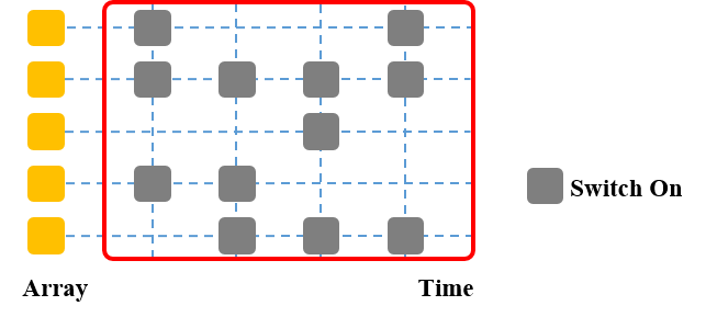
We use $\bm{p}(t)\in\{0,1\}^{N\times 1}$ to denote the random switch vector, and $p_{n}(t)$ to denote its $n$th element. When the $n$th antenna is active $p_{n}(t)=1$, and 0 otherwise. The transmitted signal of jammer array can be written as

$$\bar{\bm{v}}(t)=\bm{p}(t)\circ\bm{\alpha}(\theta_{1})r(t),$$

(10)

where the notation $\bar{\cdot}$ is used to differentiate from the counterpart of regular jamming pattern, and $\circ$ represents the Hadamard product. Compared with (1), the transmitted signal (10) of rass jammer contains modulation by the random switch vector $\bm{p}(t)$.

We assume that $p_{n}(t)$ follows a Bernoulli distribution with probability $p$, whose probability density function (PDF) is given by

$$f(p_{n}(t)|p)=\left\{\begin{array}[]{ll}p^{p_{n}(t)}(1-p)^{1-p_{n}(t)},&p_{n}(t)=0,1,\\ 0,&\mathrm{else.}\end{array}\right.$$

(11)

We also assume that $p_{n}(t)$ is independent with respect to the element index $n$ and time $t$.

Then, the jamming signal received by the $k$th radar is written as

$\displaystyle\bar{q}_{k}(t-\tau^{j}_{k}):=\bm{\alpha}^{H}(\theta_{k})(\bm{p}(t-\tau^{j}_{k})\circ\bm{\alpha}(\theta_{1}))r(t-\tau^{j}_{k}).$

(12)

Here, we define $\bar{\bm{q}}:=[\bar{q}(t-\tau^{j}_{1}),...,\bar{q}(t-\tau^{j}_{K})]^{T}\in\mathbb{C}^{K\times 1}$. Substituting the steering vector, given below (1), into (12) yields

	$\displaystyle\bar{q}_{k}(t-\tau^{j}_{k})=$	$\displaystyle\sum_{n=1}^{N}p_{n}(t-\tau^{j}_{k})r(t-\tau^{j}_{k})$		(13)
		$\displaystyle\cdot\exp^{j2\pi(n-1)d(\sin{\theta_{k}}-\sin{\theta_{1}})/\lambda}.$

Similar with (3), the received signal of the $k$-th radar under RASS jamming method is

$$\bar{x}_{k}(t)=s_{k}(t-\tau^{t}_{k})+\bar{q}_{k}(t-\tau^{j}_{k})+n_{k}(t).$$

(14)

We stack signals from all the radars, which yields the vector ${\bar{\bm{x}}}(t):=[{\bar{x}}_{1}(t),...,{\bar{x}}_{K}(t)]^{T}\in\mathbb{C}^{K\times 1}$. Here, we also assume that echoes from target $s_{k}(t-\tau^{t}_{k})$, noises $n_{k}(t)$ and the proposed jamming signals $\bar{x}_{k}(t)$ are mutually independent.

To interpret (13), we consider two cases: $k=1$ and $k\neq 1$. The former represents the main radar, where the jamming beam is directed, while the latter represents the rest radars, located in the sidelobe of the jammer’s beam pattern. When $k=1$, the coefficient $\bm{\alpha}^{H}(\theta_{k})(\bm{p}(t-\tau^{j}_{k})\circ\bm{\alpha}(\theta_{1}))$ reduces to $\bm{\alpha}^{H}(\theta_{1})(\bm{p}(t-\tau^{j}_{1})\circ\bm{\alpha}(\theta_{1}))$, which equals to $\bm{1}^{T}\bm{p}(t-\tau^{j}_{1})$, yielding the number of selected antenna units at instance $t-\tau^{j}_{1}$. This is a consequence of the fact that the jammer steers the beam towards the main radar, and also indicates that the phase of the coefficient stays unchanged even if $p_{n}(t)$ is randomly changed with respect to $t$. As a result, the antenna gain of the rass jammer against the main radar is guaranteed as long as enough antenna units are utilized. In the case of $k\neq 1$, the coefficient $\bm{\alpha}^{H}(\theta_{k})(\bm{p}(t-\tau^{j}_{k})\circ\bm{\alpha}(\theta_{1}))$ changes randomly with respect to $t$, which means that the $K-1$ passive radars will receive a randomized jamming signal. Therefore, the phase differences between jamming signals received by different radars change with respect to $t$, destroying the ‘coherence’ between radars. This property degrades the jamming elimination method used by msrs, thus better protects the target from being detected by radars.

In the next section, we will discuss the anti-suppression performance of the proposed RASS jamming method in the term of jamming cancellation method presented in Section II-A.

We derive the covariance matrix of the received signals, i.e., $\bm{\bar{R}}_{XX}:=\mathrm{E}[\bm{\bar{x}}(t)\bm{\bar{x}}^{H}(t)]$, as

$\displaystyle\bm{\bar{R}}_{XX}$

$\displaystyle=\bm{R}_{SS}+\bm{\bar{R}}_{JJ}+\sigma^{2}\bm{I},$

(15)

following the assumption that target, jamming and noise signals are uncorrelated. Here, similarly with (6), we use $\bm{\bar{R}}_{JJ}$ to denote the covariance matrix of the received jamming signals $\bar{\bm{q}}(t)$, given by

$\displaystyle\bm{\bar{R}}_{JJ}:=\mathrm{E}[\bar{\bm{q}}(t)\bar{\bm{q}}^{H}(t)].$

(16)

Comparing (15) with (8), we find that only the covariance matrix of jamming signals $\bm{\bar{R}}_{JJ}$ is changed due to the introduction of rass. Under the assumption that $\bm{p}(t)$ obeys Bernoulli distribution, we derive $\bm{\bar{R}}_{JJ}$ as stated in the following proposition:

From (17), we find that $\bm{\bar{R}}_{JJ}$ is of full rank as long as $Np(1-p)R_{rr}\bm{I}\neq\bm{0}$. Since $R_{rr}>0$, the term equals 0 if and only if $p=0$ or $1$, which means that no antenna or all the antennas are operating, respectively. In contrast to the traditional jamming pattern, i.e., when $p=1$, where the rank of $\bm{{R}}_{JJ}$ is typically 1 under the assumption that there exists only 1 jammer operating, the proposed RASS jamming method increases the rank of covariance matrix. As a result, the typical eigenprojection method used for jamming cancellation in msrs, which relies on identifying the dominant eigenvalues corresponding to jamming signals, will be affected severely.

To see this, we further discuss the eigenvalues and eigenvectors of $\bm{\bar{R}}_{XX}$ in Section III-B.

In this subsection, we apply matrix perturbation method [7] to study eigenvalues and eigenvectors of $\bm{\bar{R}}_{XX}$ in light of the counterparts of $\bm{{R}}_{XX}$.

We substitute (17) into (15), and compare the result with (5), implying

$\displaystyle\bm{\bar{R}}_{XX}$

$\displaystyle=\bm{R}_{XX}+(p^{2}-1)\bm{R}_{JJ}+Np(1-p)R_{rr}\bm{I}.$

(19)

Here, we regard $\bm{\bar{R}}_{XX}$ as a matrix generated from $\bm{{R}}_{XX}$ by adding a perturbation matrix, defined as $\Delta\bm{R}_{XX}:=(p^{2}-1)\bm{R}_{JJ}+Np(1-p)R_{rr}\bm{I}$. This facilitates revealing the relationship between eigenvalues and eigenvectors of these two matrices.

Let $\bar{\lambda}_{k}$ and $\bm{\bar{u}}_{k}$ denote the $k$-th eigenvalue and the corresponding eigenvector of $\bm{\bar{R}}_{XX}$, respectively. Here, we define $\Delta\lambda_{k}$ and $\Delta\bm{u}_{k}$ such that $\bar{\lambda}_{k}=\lambda_{k}+\Delta\lambda_{k}$ and $\bm{\bar{u}}_{k}=\bm{u}_{k}+\Delta\bm{u}_{k}$. Through the definitions of eigenvalues, we have

$$\bm{\bar{R}}_{XX}\bm{\bar{u}}_{k}=\bar{\lambda}_{k}\bm{\bar{u}}_{k},$$

(20)

or equivalently,

$\displaystyle(\bm{R}_{XX}+\Delta\bm{R}_{XX})(\bm{u}_{k}+\Delta\bm{u}_{k})$

$\displaystyle=(\lambda_{k}+\Delta\lambda_{k})(\bm{u}_{k}+\Delta\bm{u}_{k}).$

(21)

When the second order terms, i.e., $\Delta\bm{R}_{XX}\Delta\bm{u}_{k}$ and $\Delta\lambda_{k}\Delta\bm{u}_{k}$, are negligible, the perturbations in eigenvalues and eigenvectors can be approximated as [7]

	$\displaystyle\Delta\lambda_{k}$	$\displaystyle\approx\bm{u}^{H}_{k}\Delta\bm{R}_{XX}\bm{u}_{k},$		(22)
	$\displaystyle\Delta\bm{u}_{k}$	$\displaystyle\approx\bm{U}\bm{b}_{k},$

where $\bm{U}:=[\bm{u}_{1},...,\bm{u}_{K}]\in\mathbb{C}^{K\times K}$ is the eigen matrix of $\bm{R}_{XX}$ and $\bm{b}_{k}\in\mathbb{C}^{K\times 1}$ has the $i$-the entry given by $\frac{1}{\lambda_{i}-\lambda_{k}}\bm{u}^{H}_{i}\Delta\bm{R}_{XX}\bm{u}_{k}$, $i\neq k$, and the $k$-th entry being zero. Due to the length limit of this paper, we leave the proof for (22) in the journal version of this paper.

Then, the $k$-th eigenvector of $\bm{\bar{R}}_{XX}$ is given by

$$\bm{\bar{u}}_{k}=\bm{u}_{k}+\bm{U}\bm{b}_{k},$$

(23)

benefitting the analysis on JSNR, which we show in the sequel.

Under the proposed jamming pattern, we assume that msrs applies the same jamming cancellation strategy: Use the eigenvector $\bm{\bar{u}}_{1}$ corresponding to the largest eigenvalue $\bar{\lambda}_{1}$ to realize eigenprojection.

Analogy to (9), the output signal is given by

$$\bm{\bar{y}}(t)=\bm{\bar{P}}^{\perp}\bm{\bar{x}}(t)=\left(\bm{I}-\bm{\bar{u}}_{1}\bm{\bar{u}}_{1}^{H}\right)\bm{\bar{x}}(t).$$

(24)

We are now ready to evaluate the performance of the eigenprojection method. Here, we use the output JSNR as the metric, and we compare the output JSNRs under the traditional and rass jamming patterns. Particularly, we define the output JSNR under rass jamming as the following:

$\displaystyle\Omega_{R}$

$\displaystyle=\frac{\mathrm{E}[||\bm{\bar{P}}^{\perp}\bar{\bm{q}}||_{2}^{2}]}{E[||\bm{\bar{P}}^{\perp}(\bm{s}+\bm{n})||_{2}^{2}]},$

(25)

where in the numerator, the expectation is taken over $\bm{\bar{q}}$, since it is randomly changed along with time slots, while the expectation in the denominator is taken over the noise. We use subscript _R to denote the rass jamming pattern. To differentiate, we denote by $\Omega_{F}$ the counterpart under the traditional jamming pattern where the full antenna array is used. As the msrs can effectively eliminate jamming signal by eigenprojection method, the $\Omega_{F}=0$, which will be discussed later. Thus $\Omega_{R}$ represents the improvement of the proposed rass method over the traditional counterpart in the term of JSNR.

Under assumptions on the jamming pattern, we derive its JSNR in the following proposition.

From (26), we observe that the JSNR takes its maximum when $p=0.5$, suggesting the optimal jamming strategy of JSNR under Bernoulli distribution. It is also found that the JSNR increases with respect to the number of jammer’s array elements, $N$. The relationship between JSNR and the number of radars, $K$, in the numerator, is not distinct, because the energy of target echoes and noise expressed in the denominator also increase as $K$ becomes larger.

Numerical results are given in Section IV to validate the above analysis.

References

- [1] Chernyak V S. Adaptive mainlobe jamming cancellation and target detection in multistatic radar systems[C]//Proceedings of International Radar Conference. IEEE, 1996: 297-300.
- [2] Zhao S, Zhang L, Zhou Y, et al. Discrimination of active false targets in multistatic radar using spatial scattering properties[J]. IET Radar, Sonar & Navigation, 2016, 10(5): 817-826.
- [3] Yeo K, Chung Y, Yang H, et al. Reduced-dimension DOD and DOA estimation through projection filtering in bistatic MIMO radar with jammer discrimination[J]. IET Radar, Sonar & Navigation, 2017, 11(8): 1228-1234.
- [4] Ge M, Cui G, Kong L. Mainlobe jamming suppression for distributed radar via joint blind source separation[J]. IET Radar, Sonar & Navigation, 2019, 13(7): 1189-1199.
- [5] Valliappan N, Lozano A, Heath R W. Antenna subset modulation for secure millimeter-wave wireless communication[J]. IEEE Transactions on communications, 2013, 61(8): 3231-3245.
- [6] Ma D, Huang T, Liu Y, et al. A novel joint radar and communication system based on randomized partition of antenna array[C]//2018 IEEE International Conference on Acoustics, Speech and Signal Processing (ICASSP). IEEE, 2018: 3335-3339.
- [7] Champagne B. Adaptive eigendecomposition of data covariance matrices based on first-order perturbations[J]. IEEE Transactions on Signal Processing, 1994, 42(10): 2758-2770.
- [8] Feng D , Xu L , Pan X , et al. Jamming Wideband Radar Using Interrupted-Sampling Repeater[J]. IEEE Transactions on Aerospace & Electronic Systems, 2017:1-1.