Automatic feature-preserving size field
for 3D mesh generation
Abstract
This paper presents a methodology aiming at easing considerably the generation of high-quality meshes for complex 3D domains. We show that the whole mesh generation process can be controlled with only five parameters to generate in one stroke quality meshes for arbitrary geometries. The main idea is to build a meshsize field taking local features of the geometry, such as curvatures, into account. Meshsize information is then propagated from the surfaces into the volume, ensuring that the magnitude of is always controlled so as to obtain a smoothly graded mesh. As the meshsize field is stored in an independent octree data structure, the function can be computed separately, and then plugged in into any mesh generator able to respect a prescribed meshsize field. The whole procedure is automatic, in the sense that minimal interaction with the user is required. Applications examples based on models taken from the very large ABC dataset, are then presented, all treated with the same generic set of parameter values, to demonstrate the efficiency and the universality of the technique.
Keywords mesh generation, size field, background mesh, octree, feature size, proximity, curvature.
1 Introduction
Models used in industry have considerably grown in complexity over the last decades, and it is now common to mesh models with tens of thousands of faces. Ideally, a designer should create the CAD model, press the generate mesh button, and obtain in less than a minute a computational mesh valid as is for a finite element simulation. Practitioners in the field know however that things do not work out that easily in reality. Mesh generation for complex geometries is in practice a time-consuming task often involving intermediary meshes, progressively enhanced to fulfill specified meshsize and quality requirements.
The purpose of mesh generation is to build meshes with elements of controlled size and quality. We call meshsize the size of an individual finite element, evaluated by means of an appropriate scalar measure (See below). In the context of mesh adaptation, the mesh generation algorithm is constrained by a meshsize field defined on the domain to be meshed, and whose value at a point is the expected element size in the vicinity of that point. The meshsize field is usually derived from an error estimation procedure performed on the solution of a prior finite element or finite volume analysis, by requesting a smaller meshsizes at places where the discretization error is deemed large.
Yet, when solving a problem for the first time, an initial mesh has to be generated without information from a prior computation, and the meshsize field to generate that initial mesh has to be constructed from crash on basis of the geometrical data of the model only. Given a CAD model, there exist a number of theoretical prerequisites on the meshsize field to ensure a computable mesh, and this is the purpose of this paper to describe an automated algorithm to compute a meshsize field fullfilling those prerequisites a priori. The proposed approach is “user-driven”, in the sense that users should be able to generate a workable computational mesh in one click on basis of a limited number of intuitive meshing parameters, understandable by any finite element designer with no extensive background in meshing.
An isotropic meshsize field is thus a scalar function indicating the expected element size at any point in a domain to be meshed. A first design choice concerns the mathematical representation of . As our goal is to build a “first mesh”, no background mesh is yet available against which could be interpolated. A classical solution (e.g. in Gmsh [1]) is to define meshsizes directly on the geometrical entities of the model. Meshsizes can be prescribed at the vertices of the CAD model, for instance, and smoothly interpolated on model edges. They are then subsequently interpolated on surface mesh vertices. Meshsize fields interpolated this way may however be biased by geometric features of the surface mesh, such as gaps, fins or channels, which are assigned locally a small meshsize that is not expected to spread out at distance in the bulk of the volume. This approach is therefore not 100% reliable and defining the meshsize on auxiliary objects allows for a better control and prevents the aforementioned phenomenon.
Two kinds of representation for meshsize fields are encountered in the literature: namely simplicial background meshes [2, 3, 4, 5], and Cartesian grids, initially in the form of uniform grids [6], and later on in the form of non-uniform octrees [7, 8, 9]. A graphical representation of such data-structures in the two-dimensional case can be found in the first figure of [10]. It is immediately observed that uniform Cartesian grids are constrained by the smallest feature in the CAD model. As that the number of grid nodes grows cubically with the number of divisions, the memory cost of uniform Cartesian grids quickly becomes prohibitive in practice, and they were rapidly abandoned for the sake of simplicial background meshes and tree-based grids.
Both representations have however their pros and cons. Simplicial background meshes offer an accurate representation of the boundaries, and the meshsize query procedure in the three-dimensional case is reduced to a search in the two-dimensional parametric space [4, 11]. However, meshsize fields represented this way are rather sensitive to the location of the vertices in the background mesh [3], and the access time to the meshsize at a point in the background mesh might be linear in the number of nodes in the worst case. To improve on this, Chen et al. [4] proposed a walk-through algorithm based on the backward search from Shan et al. [12], although it requires a well-guessed element to quickly locate the point in the mesh, assuming an interconnection between the background mesh and the meshing algorithm.
Octrees are orientation sensitive Cartesian structures. They lack the geometrical flexibility of simplicial meshes and significative refinement may be necessary to accurately resolve surface-based information, e.g. curvatures. On the other hand, octree-based meshsize fields offer adaptive capabilities to represent quickly and easily complex meshsize distributions across the structure. Moreover, octrees offer fast access to any query points in time, where denotes the number of octants, i.e., the number of leaves in the octree. In this work, we use the octree implementation provided by p4est [13]. The serial version of p4est is used, although a scalable parallel implementation exists in the p4est library. In our implementation, a uniform meshsize is assigned to each octant in the octree, which is the most natural option with p4est.
As mentioned earlier, there are theoretical prerequisites to ensure the computability of a mesh on a given CAD model. Those prerequisites can be associated with the following five intuitive mesh parameters.
Bulk size. A bulk or default meshsize . When creating the meshsize field, the octree is refined uniformly until every octant size is smaller or equal to . This amounts to say that all meshsizes are initially set to the bulk value .
Curvature. When using piecewise linear elements, the main term of geometrical error produced by a mesh is linked with the curvature of surfaces. The local meshsizes should hence be related to the maximal curvature of the surfaces. This is done with the node density parameter that specifies the number of subdivisions of the perimeter of the local osculating circle.
Small features. A CAD model may also contain narrow or thin regions, or features, e.g. longerons that are the load-bearing components of aerospace structures. As such regions may have moderate or no curvature at all, they are likely to be overlooked by an algorithm that solely links meshsize with curvature. The thickness of narrow regions can be estimated geometrically thanks to the concept of medial axis, see Section 2.2. On this basis a third parameter is defined in our algorithm that specifies the minimal number of elements across the thickness of a narrow region. We call feature meshsize that thickness divided by . The feature meshsize and the curvature meshsize are the indicators used by our algorithm to recursively refine the octree containing the meshsize field, see Section 2.3.
Boundedness. A minimum mesh size has to be defined as a fourth parameter in our algorithm to forbid inacceptably small meshsizes, whenever curvatures are very high for instance (e.g. at corners or at the tip of a cone).
Smoothness. Accurate finite element and finite volume simulations usually require that meshsizes vary not too abruptly across the domain of computation. Yet, curvatures and feature sizes may exhibit sharp variations in practice, resulting in unacceptably large meshsize gradations. A fifth parameter is thus defined that bounds (from above) the length ratio between two adjacent edges in the mesh. In Section 2.4, we show that this condition is equivalent to limit the meshsize gradient to .
Our approach thus defines five parameters that are easy to understand by finite element practitioners, and can be given a reasonable and rather universal default value:
- •
the bulk size, or default meshsize on newly created octants, . The default value is , where is the largest dimension of the axis-aligned bounding box of the CAD model;
- •
the minimal size allowed in the final mesh, . The default value is ;
- •
the number of elements used to accurately discretize a complete circle. The default value is ;
- •
the number of element layers in thin gaps . The default value is ;
- •
the gradation, or length ratio of two adjacent edges in the final mesh, . The default value is .
This meshsize field computation has been implemented in Gmsh, which is also the tool used to generate all meshes presented in this paper. It is planned that the algorithm presented in this paper be soon integrated as a standard procedure in the meshing pipeline of Gmsh.
2 Description of the algorithm : a worked-out example
In order to illustrate the steps of the construction of the meshsize field , the CAD model of an engine block is considered as a application example (Fig. 1). This geometry contains curved surfaces and narrow features that are typical of real-life CAD models. The input data for our algorithm is a surface mesh of the CAD model, from which curvature and feature meshsize are computed. The meshsize field is generated in an independent structure in the five following steps (Fig. 1) : compute the curvature meshsize from the approximate curvature on the surface mesh of the model; compute the feature meshsize from the medial axis of the geometry; initialize the octree as the bounding box of the model and refine it uniformly until the size of all octants is at most the bulk size ; recursively refine the octree based on both the curvature and the feature meshsize, and assign the appropriate uniform meshsize in all newly created octants; smooth out the meshsize field so as to limit its gradient to . During step , the structure of the octree is not modified : only its stored meshsize field is limited to satisfy , see Section 2.4.


2.1 Approximation of surface curvatures
With piecewise linear meshes, the main term of geometrical error is due to the curvature of surfaces. Meshsize should thus be reduced in areas of high curvature. We introduce to this end the curvature meshsize . Although definition slightly varies in the literature [4, 5, 14, 15], they all rely on the subdivision of the perimeter of local osculating circles. The osculating circle at a point of a planar curve is the circle that best approximates the curve in the vicinity of the point, i.e., having same tangent and same curvature. On a smooth surface, there is thus an osculating circle in every direction, and the most critical curvature meshsize is related to the minimal radius of these circles, or reciprocally to the maximum normal curvature . Hence the following definition for the curvature meshsize :
| (1) |
with a used-defined node density. Whenever a CAD model is available in the background, surface parametrizations are at-hand and normal curvature can be obtained through the solid modeller’s API. As far as our algorithm i concerned however, input data is a triangulation and normal curvatures are approximated following the tensor averaging methodology described by Rusinkiewicz [16], briefly recalled here with their notations.
Let denote an orthonormal basis in the tangent plane at a point of a smooth surface, and be an arbitrary direction in that plane. The normal curvature at in the direction is given by
where denotes the second fundamental form. The eigenvalues and of the symmetric matrix , known as the principal curvatures, are the maximum and miminum values of normal curvature at . Since we need to define the curvature meshsize (1), our goal is thus to build an approximation of at each vertex of the surface mesh.
The idea in [16] is to compute first on the triangles, and average them over adjacent triangles to obtain the needed per-vertex information. We start by computing per-vertex normal vectors by averaging the normals of all faces adjacent to each vertex. On each triangle, an arbitrary orthonormal coordinate system is then defined. The components of the quadratic form in that basis read
They can be evaluated as where the shape operator is the directional derivative of the normal vector along a direction in the tangent plane. One has now the following finite difference approximation
| (2) |
with the edge from vertex to vertex .
On the other hand, the edge , regarded as a vector, admits a decomposition in that basis and, because the second fundamental form is a bilinear form, it follows that
| (3) |
Combining (2) and (3), and proceeding the same way for yields the following pair of relationships between the components of :
Repeating the same procedure for the two remaining edges of the triangle, one ends up with a system of 6 equations for 3 unknowns, which can be solved using a least square method.
This per-face approximation of is expressed in the local basis . In order to now combine the contributions of all triangles adjacent to a vertex , one further orthonormal basis is defined in the plane perpendicular to the normal vector at . The basis is defined as the basis slightly tilted (i.e., rotated) to be coplanar with , and the contribution of the face to can then be expressed in the rotated basis as
As for the normals, the contributions of all triangles adjacent to the vertex are then averaged to finally obtain . Finally, the curvature meshsize of the vertex is computed from the maximal eigenvalue of using (1) (Fig. 2(a)).


2.2 Feature size
Whenever two surfaces with moderate or no curvature are close to each other but the distance between them is smaller than the meshsize, the mesh generator will place only one element in the gap between those surfaces. In many engineering applications like solid mechanics or fluid mechanics, having only one element in a gap means that both sides are connected by one single mesh edge. If Dirichlet boundary conditions are applied, such as a non-slip boundary condition, the gap is then essentially closed, leading to an unwanted change of the domain topology. Note that a posteriori error estimation will not detect large errors in those closed gaps where the solution is essentially constant.
Hence, special care should be given to such narrow geometrical regions, where curvature information alone is not enough to determine a suitable meshsize field. To this end, we define the feature size as a measure of the local gap thickness (Fig. 3(a)). If is the boundary of a volume , , , is defined as twice the distance between and the medial axis of volume . If a surface bounds two volumes, then the minimum feature size is chosen. The feature meshsize at the considered vertice, now, is the feature size devided by the desired number of element layers in narrow regions , i.e., . The feature meshsize is thus in a similar relationship to the feature size than the curvature meshsize was to the maximum principal curvature .
The evaluation of the feature size thus requires computing an approximation of the medial axis of all volumes in the computational domain. The medial axis of a volume , also referred to as its skeleton, is defined as the set of points having more than one closest point on its boundary . Equivalently, the medial axis is the set of the centers of all spheres tangent to in two or more points, and the feature size is twice the radius of the sphere tangent at .
We rely on the algorithm Medial introduced by Dey and Zhao [17] to compute a discrete approximation of the medial axis. The algorithm is based on the Voronoï diagram of the vertices of the surface mesh, and it has suitable convergence properties in the sense that the output set of facets converges to the medial axis as the surface mesh density increases. It takes as input data a Delaunay tetrahedrization of the vertices of the surface mesh only, i.e., a set of tetrahedra, often called empty mesh, filling the computational domain and whose nodes all lie on the surfaces. The rationale behind the algorithm Medial can be sketched as follows with the notations of Dey and Zhao. In 2D, the vertices of the Voronoï cells that are dual of an empty mesh give straigth away an approximation of the medial axis. The same is however not always true in 3D, because sliver tetrahedra of the empty mesh can persist close to the boundary as the surface mesh is refined. However, by pruning as explained below the Voronoï vertices dual of these sliver tetrahedra, a subset of Voronoï vertices called poles can be defined that do approximate the medial axis (Fig. 2(b)). Given the Voronoï cell dual of a surface vertex (Fig. 3(a)), the corresponding pole is defined as the Voronoï vertex that is the most distant from . Each surface vertex is thus associated with a pole , and then with a pole vector that approximates the normal to at (Fig. 3(b)).
The plane passing through with normal intersects edges of the Voronoï cell, and the Delaunay facets dual to these edges are pictorially called the umbrella of by Dey and Zhao (Fig. 3(b), in light grey).
Triangles of the umbrella are used to select some of the Delaunay edges adjacent to whose dual facets will eventually form the discrete medial axis. The idea is to select Delaunay edges that make a sufficiently large angle with the triangles of the umbrella, or are significantly longer than the circumradius of these triangles. Condition measures how normal the edge is to the umbrella and is referred to as the angle condition. The edge should make an angle larger than with each triangle of the umbrella, or conversely, an angle smaller than with their normal vector. In practice, we evaluate [17] :
where is a vector parallel to the edge , denotes a triangle in and the threshold angle is set to . Condition ensures that edges of the surface mesh are removed. It does so by selecting long edges for which the angle condition has failed, and is referred to as the ratio condition. In practice, only edges at least times longer than the circumradius of the triangles in are considered, and the condition reads [17] :
The numerical values for parameters and are those suggested by Dey and Zhao. They yield a good approximation of the medial axis for a large variety of geometries. If a Delaunay edge satisfies either of these two conditions, its dual Voronoï facet is added to a set , forming the approximate medial axis. Consider the three mesh vertices connected to through a Delaunay edge on Figure 3(b). Edge makes a large angle with the triangles of the umbrella, and edge is several times longer than the largest circumradius : both are added to the set dual to . Edge is a short surface edge mesh lying flat to the umbrella, and is thus removed from the list of candidate edges.
In our meshsize field computation, we need not compute the dual facet to edges in : for each Delaunay edge satisfying the angle or ratio conditions, the local feature size is directly given by the edge length . Meshsize at both vertices and is thus defined as the edge length divided by the desired number of element layers in features :
The meshsize on the octants containing these vertices is then lower bounded if necessary :

The medial axis also contains the centers of spheres with radius vanishing to zero in all angles and corners of the volume (Fig. 4(a)). Dual edges in these corners are smaller than the feature size one wants to identify, and they should thus be disregarded to avoid spurious small meshsize in such areas. In practice, an edge making an angle larger than with either one of the normal vectors and at its ends is also filtered out (Fig. 4(b)).
The quality of the approximation of the medial axis is directly related to the node density of the surface mesh. As pointed out by Dey and Zhao, the surface mesh should be an -sample, i.e., vertices should have neighbours within a distance , where is the feature size and is small. Of course, as the aim is here precisely to compute the feature size, it is not known beforehand whether or not the input surface mesh is a -sample. A first solution is to measure beforehand the most critical feature size of the CAD model, then generate a uniform mesh with constant meshsize , typically with as suggested in [17]. The characteristic size of the input surface mesh is then constrained by the smallest feature in the geometry, which may result in an expensive size field computation. While we could certainly adjust the meshsize of the input mesh to be only in the small features, this would amount to manually specify the meshsize field, which we want to avoid. To circumvent this, one can compute an initial meshsize field based on a reasonably fine uniform mesh, then perform the mesh generation from this field. This intermediary mesh will include an initial refinement in the small features, and will be a better candidate for the final meshsize field computation.


The resulting medial axis for our block example after the two filtering operations is shown on Figure 5(a). Taking into account the local feature size allows for a refined mesh in small features of the geometry, especially in areas with zero curvature, which would be overlooked otherwise (Fig. 6, see also Fig. 11 for the volume mesh).


2.3 Octree initialization and refinement
The meshsize field over the domain to be meshed is now built as an octree structure. The initial octant is defined as the axis-aligned bounding box of the surface mesh, stretched in all three dimensions by a factor . In order to ensure a suitable gradation in the mesh, the main idea in leading the refinement of the octree is that the dimension of each octant should eventually be representative of the local meshsize. The octree is then first subdivided recursively and uniformly until the size of each octant is at most the bulk size , and the local meshsize value affected to the octants created during this initial step are set to . The octree is then further refined on basis of the curvature meshsize and the feature meshsize . This information, which is available on the surfaces, has to be transfered to the octree, which is three-dimensional structure. One needs for that to detect efficiently the intersections between octants and the surface mesh. To this end, the three-dimensional bounding box of each triangle of the surface mesh is added to an R-Tree [18], a data structure used for spatial access methods (Fig. 5(b)) which acts here as the intermediary between the geometry and the octree. More specifically, the R-Tree provides for each octant of index a list of triangles whose bounding box intersects the octant. The octant with index is then divided until it becomes smaller than the minimal meshsize ( or ) at the vertices of all triangles in . Whenever an additional user-defined meshsize function is provided, this additional constraint is also taken into account at this level. The octant size being bounded from below by the user-defined minimal meshsize , octants are thus subdivided until the condition
| (4) |
is met everywhere in the octree.
Once this refinement is completed, the octree is balanced to ensure a maximum 2:1 level ratio between two octants across adjacent faces (Fig. 7), that is, the levels of two octants on each side of a face should not differ by more than one unity. This balancing is necessary to obtain suitable stencils for finite difference computations during the gradient limiting step, see Section 2.4. It is performed by p4est. Newly created octants having an intersection with the surface mesh are assigned the meshsize determined by (4), otherwise the meshsize is set to the bulk size (Fig. 10(a)). At this stage, the meshsize field features large variations, and a smoothing step is required to end up with a meshsize field suitable for high-quality mesh generation.


2.4 Regularization
Large meshsize gradients may be the cause of low quality finite element solutions. In solid mechanics e.g., they may be the cause of excessive values of strains when a very small element is adjacent to a large one. One of the goals of our approach is to ensure that two adjacent edges in the mesh have their length ratio that are controlled by a user-defined factor , called the regularization parameter. We now show that this amounts to limiting the size field gradient by a factor :
| (5) |
This condition may look odd, as one would expect a linear meshsize field to yield a linear progression of ratio of element sizes, instead of a geometric progression. Let us consider a standard boundary layer mesh (Fig. 8) defined as follows : a wall size defines thickness of the first element layer and a ratio defines the geometric progression of element sizes. The -th layer of elements thus has a size . Let us show that a geometric progression of element sizes actually corresponds to an affine size field. Let be the vertical distance to the wall. The coordinate corresponding to the bottom of the -th layer is given by
We can thus compute:
Since , we have
and the mesh size is affine with respect to the distance to the wall, so its gradient is constant and equal to . A similar computation by Chen et al. [ref] leads to the condition : both conditions are very close for typical values of 11 1 We have . As pointed out by [ref], this one-dimensional analysis is not sufficient to ensure a global gradation in the mesh. Indeed, when storing the size function in a background mesh, constraining the size gradient along edges only ensures the expected gradation along the element edges but allows for size variation in the interior of the elements in 2D and 3D. To constrain the size gradient on both the edges and the interior, one has to iterate over the edges of the background mesh and correct locally the size information stored at the nodes [4, 5]. This results in a size function that satisfies (5) in a mesh-dependent fashion [10]. This is not necessary in our methodology, since the size function is stored in a balanced octree : condition (5) is satisfied everywhere in the volume by iterating over the octants until convergence. This ensures the gradation is respected in the interior of the elements.
Gradient computation by finite difference. The regularization parameter here introduced limits the maximum ratio between two adjacent edges of the mesh. To ensure that, we iterate over the octants to limit until
| (6) |
everywhere, with . For each octant, we take advantage of the 2:1 balancing provided by p4est to compute the gradient with a cell-centered finite difference scheme. Since the octree is balanced, only three different stencils are necessary to approximate the derivatives. To use p4est terminology, one side of a face between two octants is said to be either full (F) or hanging (H), depending if the octant on that side is a leaf or is itself subdivided, respectively. The three stencils (Fig. 9) are then FFF, FFH, HFH, the all-hanging case being divided in multiple all-full stencils. To evaluate the derivatives of the sizing function at the center of the middle octant along, say, the x-direction, we use the following Taylor approximation :
| (7) |
where denotes the average of the size stored in the four adjacent octants to a hanging face, and is the sum of the half-lengths of octants on each side of a face. For the all-full stencil, and is a constant step equal to the length of an octant, so that this approximation reduces to the usual second-order centered scheme. By taking the average size in the hanging case, we decouple the equations to solve for the discrete approximation of the size gradient, and avoid solving a least-square problem at each octant and at each iteration.
Size limitation. The computed gradient is then used to limit the size field. For any two adjacent octants with gradient larger than , larger sizes are limited in order to satisfy condition (5) : let and denote the size stored on the octants, with . The larger size is corrected using the linear extrapolation :
| (8) |
This expression is the discretized version of the steady-state solution to the Hamilton-Jacobi equation proposed by Persson [10] in their continuous formulation of the gradient limiting problem, ensuring size limitation is propagated in the direction of increasing values. Smaller sizes are left unchanged, so that sharp features of the geometry are preserved in the size function and are not overlooked during surface or volume meshing. The smoothing is performed iteratively in the three directions, until the constraint is satisfied everywhere in the octree, propagating the small sizes and yielding a continuous size field (Fig.10(b)).


2.5 Size query in the octree
Size queries are performed by Gmsh to evaluate the size at different locations on parametrized curves, surfaces and volumes during the meshing process. The implementation of queries routine in the octree is provided by p4est. Since both the size and its gradient are known in each octant, the size at the query point is approximated by a first-order Taylor expansion, that is :
where and denote the size at and the coordinate of the center of the octant, respectively.
3 Results
To illustrate our methodology, our algorithm has been applied on a large variety CAD models. The models were found at different locations: GrabCAD (https://grabcad.com/), the ABC Dataset model library [19] and Gmsh’s benchmarks suite. For each of the following test cases, we start by tessellating the CAD model using a uniform mesh size over the whole geometry. The resulting triangular mesh is the input of our algorithm. We then compute (i) surface curvatures and (ii) the approximate medial axis. Those two informations are processesed to build a size field as described in the previous sections of the paper. The octree is stored on disk in the native p4est format and is loaded as a background field in Gmsh 22 2 gmsh foo.geo -bgm foo.p4est.
This sections aims at showing that our approach is both efficient and accurate. As far as efficiency is concerned, we distinguish the CPU time dedicated to queries in the octree and the CPU time devoted to the construction of the octree. We then compare the sum of those two to the remaining time for meshing. Note here that the last evolution of Gmsh’s 3D mesh generator is extremely efficient[20]. We show that the new size field does not change orders of magnitude in the meshing time. In other word, seconds remain seconds and do not become minutes. With regard to accuracy, we check wether critical parameters of our approach are taken ino account accurately. Discrete gradients of mesh sizes are compared with their limit value . The number of elements in small gaps is checked to be close to . Finally, the efficiency index of size fields, which measures the discrepancy between adimensional edge lengths and their ideal values , is presented.
All computations are run on a laptop with Intel Core i7 8750h CPU (2.2 GHz) and 16Gb memory. Execution times for two selected test cases can be found in the table hereafter.
The parameters chosen for the size field constructionss are :
- •
the bulk size is set to , where denotes the maximum dimension of the axis-aligned bounding box of the model;
- •
the minimum size is set to ;
- •
the node density is set to ;
- •
the number of layers in geometric features is set to ;
- •
the gradation is set to .
3.1 Surface and volume meshing
Running example. We first present the resulting meshes of the engine block test case. The geometry, while being relatively simple, has all features that should be captured by our approach: it presents entities of variable radii of curvature each endowed with a specific curvature meshsize. The CAD model is mostly an assemblage of thin components such as thin cylinders and narrow fins surrounding the main cylinder: feature meshsize is thus the dominant meshing criterion overall. Surface meshes are presented in Section 2, and show the impact of the feature meshsize (Fig. 6). On the left part of Figure 6, the meshsize field is based only on the curvature meshsize : we see that only one or two elements are generated in the narrow fins, whose meshsize is mostly defined by the radius of curvature of the inner cylinder. On the right part of Figure 6, feature meshsize is included in the meshsize field and we observe layers in the fins. Figure 11 reveals the tetrahedral mesh and confirms that meshsize specifications are respected inside the volume by the meshing tool. Meshsize in curved areas, such as corners, is constrained by curvature rather than geometric features, since branches of the medial axis were removed in their vicinity. This results in a smaller meshsize defined by the node density (zooms 2 and 3). Meshsize in the thin cylinders and the fins is computed to fit 4 layers of elements (zooms 1, 4, 5, 6 and 7).

Sport bike engine. Our second test case is the four-cylinder engine of a Honda™ CBR600F4i sport bike, accessed from GrabCAD33 3 https://grabcad.com/library/honda-cbr600-f4i-engine-1. The model is composed of thin areas such as pipes, gears and plates, and of a large number of features overall, making it a interesting test case for our algorithm. Unfortunately, the volume enclosed is not "air-tight", and can not be meshed without repairing the CAD model, hence only surface meshes are presented for this example. The resulting surface meshes accurately capture areas of higher curvature (Fig. 12, left) as well as the small features (Fig. 12, right and Fig. 13), demonstrating the robustness of our algorithm on such large CAD models.


Space shuttle. This model illustrates the influence of the node density and the gradation on the resulting mesh. To clearly show the mesh gradation on flat surfaces, surface proximity was not considered to compute these size fields : only curvature was taken into account. As expected, larger values of will result in more elements on the local osculating circle to a surface, resulting in a finer mesh (Fig.14). Similarly, a gradation close to will limit the geometric progression in the mesh size, also resulting in a finer and homogeneous mesh (Fig.15). The parameter directly translates into the desired mesh density, and is thus dependent of the aimed application for the mesh. The gradation however, has similar values for different ranges of applications : typically, we recommend using between and for fluid mechanics computations, for solid mechanics and up to for electromagnetism numerical simulations. The value of is also suited for boundary layer meshes in fluid mechanics. [refs?]


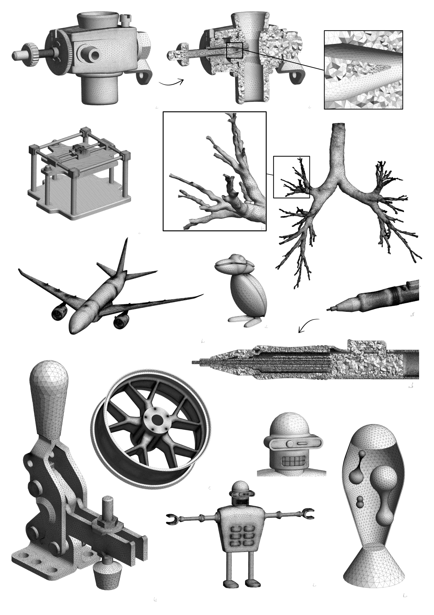
Various geometries. Finally, we tested our algorithm with the same parameters on various CAD model retrieved from GrabCAD, the ABC Dataset library and the Gmsh benchmarks library (Fig. 16). On all models, accurate size fields were computed in a few seconds to a few minutes, yielding smooth meshes suitable for numerical simulations and saving precious time to the user. Note that feature size computation was not enabled for all models (e.g. for the lava lamp).
3.2 Adequation between the mesh and the size field
Efficiency index. The resulting mesh should be as close as possible as a unit mesh in the metric field associated to the isotropic sizing function [21], i.e. the edges lengths should be as close as 1 when measured in the given metric. Since we are dealing with the discrete counterpart of this continuous mesh framework, we consider that the size specification is respected when the edges lie in . To evaluate the adequation between the generated mesh and the prescribed size field, we define an efficiency index. Let be the length of an edge computed in the local metric and the number of edges in the mesh. The efficiency index of a mesh is defined as the exponential to one of all the edges length in the mesh, that is :
with if and if . The efficiency index thus lies in , the upper bound being reached for a unit mesh. We run our algorithm on close to two hundred CAD models and computed the efficiency index (Fig. 17), whose median is slightly above . This shows that the size field given to the meshing tool is realistic, as it can generate almost unit edges for the given metric field.


Discrete gradation. The resulting mesh should feature a geometric progression in adjacent edges lengths with a ratio up to . Instead of monitoring the maximum edge ratio at every vertices of the final mesh, we use a looser indicator defined on the edges. The discrete gradation measures the progression between the average edges lengths at both vertices of each edge . Let and denote the vertices of and the average edge length at vertex . We define the discrete gradation at edge as follows :
In the same way that the efficiency index is a global indicator for a given mesh, we define an average discrete gradation as the average of over all edges of the mesh. The average discrete gradation should be close to the user-defined gradation . In our results over the same sample of meshes, the discrete gradation is very close to the required gradation, although it lies slightly above or below depending on the value of (Fig. 18).


Quality measure. Finally, the chosen quality criterion for the tetrahedral meshes is the ratio of the inscribed radius to the circumscribed radius :
The resulting mesh for the engine block example contains almost no element with quality below , and shows a typical distribution for a 3D mesh.
3.3 Execution time
The execution time for the engine block and the Honda engine are given in Table 1. The size field time is split between the main steps of the algorithm : insert the bounding boxes of the triangles of the surface mesh in the RTree, compute the approximated curvature with a least square method, initialize the root octant and refine the octree, compute the medial axis of the geometry, and limit the size gradient to . Computing the medial axis requires the Delaunay tetrahedrization of the points from the surface mesh : this step is detailed and included in the time associated to the medial axis computation. The step "Others" includes all the secondary steps, such as splitting the mesh into faces before computing curvature.
To limit the size gradient, we iterate over the octants until condition (4) is satisfied in all three directions. This step is dependent on the depth of the octree, hence on the minimum size , the node density and the curvature of the surface mesh given as input. A highly curved region of the model due to a poor resolution of the surface mesh will result in high density in the octree, increasing the smoothing time. This can generally be circumvented by first generating a slightly refined surface mesh, which can be computed quickly and will rule out these extreme curvature magnitudes. Computation time for the medial axis, on the other hand, is linear with the number of nodes of the input mesh : this is indeed observed in Table 1.
| Block | Honda engine | ||||
| Time () | % | Time () | % | ||
| Create size field | Insert surface mesh in RTree | 0.47 | 3.0 % | 2.84 | 1.3 % |
| Compute curvature | 0.36 | 2.3 % | 1.13 | 0.5 % | |
| Create and refine octree | 0.96 | 6.1 % | 20.59 | 9.1 % | |
| Compute medial axis | 7.19 | 45.7 % | 39.28 | 17.4 % | |
| incl. Delaunay tetrahedrization of surface mesh | 0.61 | 3.9 % | 3.19 | 1.4 % | |
| Limit size gradient | 5.85 | 37.1 % | 154.21 | 68.3 % | |
| Others | 0.69 | 4.3 % | 7.08 | 3.1 % | |
| Total | 15.75 | 100.0 % | 225.87 | 100.0 % | |
| Mesh model | Mesh 1D entities | 2.48 | 2.5 % | 119.80 | 30.2 % |
| Mesh 2D entities | 25.68 | 25.6 % | 277.35 | 69.8 % | |
| Mesh 3D entities | 72.12 | 71.9 % | / | / | |
| Total | 100.3 | 100.0 % | 397.33 | 100.0 % | |
| including Size queries | 65.13 | 64.9 % | 169.41 | 42.6 % | |
| # of curves in the CAD model | 1584 | 53,237 | |||
| # of faces in the CAD model | 533 | 21,771 | |||
| # of nodes in input surface mesh | 145,024 | 868,980 | |||
| # of elements in input surface mesh | 290,116 | 1,737,310 | |||
| # of octants | 670,566 | 14,615,413 | |||
| # of triangles in final surface mesh | 573,808 | 4,605,010 | |||
| # of tetrahedron in final volume mesh | 2,716,170 | / | |||
4 Conclusion
We have presented a methodology to generate an accurate size field in an automatic way, storing the sizing information in an octree. Five user parameters are required to generate a mesh suitable for numerical simulations, two of which being the minimum and the maximum, or bulk, size, whose value is assigned based solely on the characteristic dimension of the CAD model. This leaves the user with only three parameters to choose in order to tune the mesh density. This tool eliminates the tedious operation that is assigning by hand the mesh size on all geometric entities of a CAD model, thus saving precious time. Special care was given to the small features of the geometry : through an approximate medial axis computation, we ensure multiple layers of elements are always generated in narrow regions. This is particularly useful in simulations where Dirichlet boundary conditions are applied. To illustrate our size field computation, we applied our algorithm on a variety of CAD models : in each application, the proposed method accurately targets the regions of higher curvature and adapts the mesh size accordingly. Small features are identified through the medial axis, such that the final meshes include element layers in possible channels in the geometry. For all of the test cases, surface and volume meshes can be obtained in a robust and automatic fashion, and are adapted to the features of the geometric model. This tool will soon be integrated in the standard Gmsh pipeline. Future work will focus on extending to anisotropic size propagation, as well as interaction between the octree and numerical solutions to include a posteriori error estimation in the size field design.
5 Acknowledgements
The authors would like to thank the Belgian Fund for Scientific Research (FRIA-FNRS) for their support. Financial support from the Simulation-based Engineering Science (Génie Par la Simulation) program funded through the CREATE program from the Natural Sciences and Engineering Research Council of Canada is also gratefully acknowledged.
References
- [1] Christophe Geuzaine and Jean-François Remacle. Gmsh: A 3-d finite element mesh generator with built-in pre-and post-processing facilities. International journal for numerical methods in engineering, 79(11):1309–1331, 2009.
- [2] Alexandre Cunha, Scott Canann, and Sunil Saigal. Automatic boundary sizing for 2d and 3d meshes. ASME APPLIED MECHANICS DIVISION-PUBLICATIONS-AMD, 220:65–72, 1997.
- [3] Steven J Owen and Sunil Saigal. Neighborhood-based element sizing control for finite element surface meshing. In 6th International Meshing Roundtable Proceedings, pages 143–154, 1997.
- [4] Jianjun Chen, Zhoufang Xiao, Yao Zheng, Jianjing Zheng, Chenfeng Li, and Kewei Liang. Automatic sizing functions for unstructured surface mesh generation. International Journal for Numerical Methods in Engineering, 109(4):577–608, 2017.
- [5] Jianjun Chen, Zhiwei Liu, Yao Zheng, Peng Zheng, Jianjing Zheng, Zhoufang Xiao, and Chuang Yu. Automatic sizing functions for 3d unstructured mesh generation. Procedia engineering, 203:245–257, 2017.
- [6] Shahyar Pirzadeh. Structured background grids for generation of unstructured grids by advancing-front method. AIAA journal, 31(2):257–265, 1993.
- [7] Jin Zhu, Ted D Blacker, and Rich Smith. Background overlay grid size functions. In IMR, pages 65–73, 2002.
- [8] Ko-Foa Tchon, Mohammed Khachan, François Guibault, and Ricardo Camarero. Three-dimensional anisotropic geometric metrics based on local domain curvature and thickness. Computer-Aided Design, 37(2):173–187, 2005.
- [9] William Roshan Quadros, Ved Vyas, Mike Brewer, Steven James Owen, and Kenji Shimada. A computational framework for automating generation of sizing function in assembly meshing via disconnected skeletons. Engineering with Computers, 26(3):231–247, 2010.
- [10] Per-Olof Persson. Mesh size functions for implicit geometries and pde-based gradient limiting. Engineering with Computers, 22(2):95–109, 2006.
- [11] Jianjun Chen, Bingwan Cao, Yao Zheng, Lijun Xie, Chenfeng Li, and Zhoufang Xiao. Automatic surface repairing, defeaturing and meshing algorithms based on an extended b-rep. Advances in Engineering Software, 86:55–69, 2015.
- [12] JL Shan, YM Li, YQ Guo, and ZQ Guan. A robust backward search method based on walk-through for point location on a 3d surface mesh. International journal for numerical methods in engineering, 73(8):1061–1076, 2008.
- [13] Carsten Burstedde, Lucas C. Wilcox, and Omar Ghattas. p4est: Scalable algorithms for parallel adaptive mesh refinement on forests of octrees. SIAM Journal on Scientific Computing, 33(3):1103–1133, 2011.
- [14] M Turner, D Moxey, and J Peiró. Automatic mesh sizing specification of complex three dimensional domains using an octree structure.
- [15] Frank Deister, Udo Tremel, Oubay Hassan, and Nigel P Weatherill. Fully automatic and fast mesh size specification for unstructured mesh generation. Engineering with computers, 20(3):237–248, 2004.
- [16] Szymon Rusinkiewicz. Estimating curvatures and their derivatives on triangle meshes. In Proceedings. 2nd International Symposium on 3D Data Processing, Visualization and Transmission, 2004. 3DPVT 2004., pages 486–493. IEEE, 2004.
- [17] Tamal K Dey and Wulue Zhao. Approximating the medial axis from the voronoi diagram with a convergence guarantee. Algorithmica, 38(1):179–200, 2004.
- [18] Norbert Beckmann, Hans-Peter Kriegel, Ralf Schneider, and Bernhard Seeger. The r*-tree: an efficient and robust access method for points and rectangles. In Acm Sigmod Record, volume 19, pages 322–331. Acm, 1990.
- [19] Sebastian Koch, Albert Matveev, Zhongshi Jiang, Francis Williams, Alexey Artemov, Evgeny Burnaev, Marc Alexa, Denis Zorin, and Daniele Panozzo. Abc: A big cad model dataset for geometric deep learning. In The IEEE Conference on Computer Vision and Pattern Recognition (CVPR), June 2019.
- [20] Célestin Marot, Jeanne Pellerin, and Jean-François Remacle. One machine, one minute, three billion tetrahedra. International Journal for Numerical Methods in Engineering, 117(9):967–990, 2019.
- [21] Pascal Jean Frey and Paul-Louis George. Maillages: applications aux éléments finis. Hermès Science Publications, 1999.