Neural-PDE: A RNN based neural network for solving time dependent PDEs Volume: 0Issue: 0

A time-dependent partial differential equation is an equation of the form:

$$u_{t}=f(x_{1},\cdots,u,\frac{\partial u}{\partial x_{1}},\cdots,\frac{\partial u}{\partial x_{n}},\frac{\partial^{2}u}{\partial x_{1}\partial x_{1}},\cdots,\frac{\partial^{2}u}{\partial x_{1}\partial x_{n}},\cdots,\frac{\partial^{n}u}{\partial x_{1}\cdots\partial x_{n}})~,$$

(2.1.1)

where $u=u(x_{1},...,x_{n},t)$ is known, $x_{i}\in\mathbb{R}$ are spatial variables, and the operator $f$ maps $\mathbb{R}^{N}\mapsto\mathbb{R}$. For example, consider the parabolic heat equation: $u_{t}=\alpha^{2}\Delta u$, where $u$ represents the temperature and $f$ is the Laplacian operator $\Delta$. Eq. (2.1.1) can be solved by finite difference methods, which are briefly reviewed below for the self-completeness of the paper.

Consider using a finite difference method (FDM) to solve a two-dimensional second-order PDE of the form:

$$u_{t}=f(x,y,u_{x},u_{y},u_{xx},u_{yy}),\quad(x,y)\in\Omega\subset\mathbb{R}^{2},\quad t\in\mathbb{R}^{+}\cup\{0\}~,$$

(2.2.1)

with some proper boundary conditions. Let $\Omega$ be $\Omega=[x_{a},x_{b}]\times[y_{a},y_{b}]$, and

$\displaystyle u_{i,j}^{n}=u(x_{i},y_{j},t_{n})$

(2.2.2)

where $t_{n}=n\delta t,\;0\leq n\leq N$, and $\delta t=\frac{T}{N}\;$ for some large integer $N$. $x_{i}=i\delta x,\;0\leq i\leq N_{x}$, $\delta x=\frac{x_{a}-x_{b}}{N_{x}}\;$.  $y_{j}=j\delta y,\;0\leq j\leq N_{y}$, $\delta y=\frac{y_{a}-y_{b}}{N_{y}}\;$. $N_{x}$ and $N_{y}$ are integers.

The central difference methods approximate the spatial derivatives as follows (thomas2013numerical):

	$\displaystyle u_{x}(x_{i},y_{j},t)$	$\displaystyle=\frac{1}{2\delta x}(u_{i+1,j}-u_{i-1,j})+\mathcal{O}(\delta x^{2})~,$		(2.2.3)
	$\displaystyle u_{y}(x_{i},y_{j},t)$	$\displaystyle=\frac{1}{2\delta y}(u_{i,j+1}-u_{i,j-1})+\mathcal{O}(\delta y^{2})~,$		(2.2.4)
	$\displaystyle u_{xx}(x_{i},y_{j},t)$	$\displaystyle=\frac{1}{\delta x^{2}}(u_{i+1,j}-2u_{i,j}+u_{i-1,j})+\mathcal{O}(\delta x^{2})~,$		(2.2.5)
	$\displaystyle u_{yy}(x_{i},y_{j},t)$	$\displaystyle=\frac{1}{\delta y^{2}}(u_{i,j+1}-2u_{i,j}+u_{i,j-1})+\mathcal{O}(\delta y^{2})~.$		(2.2.6)

To this end, the explicit time-stepping scheme to update next step solution $u^{n+1}$ is given by:

	$\displaystyle u_{i,j}^{n}\approx U_{i,j}^{n+1}$	$\displaystyle=U_{i,j}^{n}+\delta tf(x_{i},y_{j},U_{i,j}^{n},U_{i,j-1}^{n},U_{i,j+1}^{n},U_{i+1,j}^{n},U_{i-1,j}^{n})~,$		(2.2.7)
		$\displaystyle\equiv\mathbf{F}(x_{i},y_{j},\delta x,\delta y,\delta t,U_{i,j}^{n},U_{i,j-1}^{n},U_{i,j+1}^{n},U_{i+1,j}^{n},U_{i-1,j}^{n})~,$		(2.2.8)

where $U_{i,j}^{n}$ is the numerical solution at grid point $(x_{i},y_{j},t_{n})$.

Apparently, the finite difference method (2.2.7) for updating $u^{n+1}$ on a grid point relies on the previous time steps’ solutions, supported on the grid point and its neighbours. The scheme (2.2.7) updates $u^{n+1}_{i,j}$ using five points of $u^{n}$ values (see Figure 1).

Similarly, the finite element method (FEM) approximates the new solution by calculating the corresponded mesh cell coefficient, which is updated by its related nearby coefficients on the mesh.

From this perspective, one may regard the numerical schemes for solving time-dependent PDEs as methods catching the information from neighbourhood data of interest.

Finite element method (FEM) is a powerful numerical method in solving PDEs. Consider a 1D wave equation of $u(x,t)$:

		$\displaystyle u_{tt}-v^{2}u_{xx}=f,\quad x\in[a,b]\equiv\Omega\subset\mathbb{R},\quad t\in\mathbb{R}^{+}\cup\{0\}~,$		(2.3.1)
		$\displaystyle u_{x}(a,t)=u_{x}(b,t)=0~.$		(2.3.2)

The function $u$ is approximated by a FEM function $u_{h}$ :

$\displaystyle u(x,t)\approx u_{h}(x,t)$

$\displaystyle=\sum_{i=1}^{N}a_{i}(t)\psi_{i}(x)$

(2.3.3)

where $\psi_{i}\in V$ is the basis functions of some FEM space $V$, and $a_{i}^{n}$ denotes the coefficients. $N$ denotes the degrees of freedom.
Multiply the equation with an arbitrary test function $\psi_{j}$ and integral over the whole domain we have:

$\displaystyle\int_{\Omega}u_{tt}\psi_{j}\ dx+v^{2}\int_{\Omega}\nabla u\nabla\psi_{j}\ dx=\int_{\Omega}f\psi_{j}\ dx$

(2.3.5)

and approximate $u(x,t)$ by $u_{h}$:

	$\displaystyle\sum_{i}^{N}\frac{\partial^{2}a_{i}(t)}{\partial t^{2}}\underbrace{\int_{\Omega}\psi_{i}\psi_{j}\ dx}_{\mathbf{M}_{i,j}}+v^{2}\sum_{i}^{N}a_{i}(t)\underbrace{\int_{\Omega}\nabla\psi_{i}\nabla\psi_{j}\ dx}_{\mathbf{A}_{i,j}}=\underbrace{\int_{\Omega}f\psi_{j}}_{\mathbf{b}}\ dx~,$		(2.3.7)
	$\displaystyle\equiv\mathbf{M}^{T}\mathbf{a}_{tt}+v^{2}\mathbf{A}^{T}\mathbf{a}=\mathbf{b}~.$		(2.3.8)

Here $\mathbf{M}$ is the mass matrix and $\mathbf{A}$ is the stiffness matrix, $\mathbf{a}=(a_{1},..,a_{N})^{t}$ is a $N$ vector of the coefficients at time $t$. The central difference method for time discretization indicates that (johnson2012numerical):

$\displaystyle\mathbf{a}^{n+1}$

$\displaystyle=2\mathbf{a}^{n}-\mathbf{a}^{n-1}+\mathbf{M}^{-1}(\mathbf{b}-v^{2}\mathbf{A}^{T}\mathbf{a}^{n})~.$

(2.3.9)

This leads to

$\displaystyle u^{n+1}$

$\displaystyle\approx u_{h}^{n+1}=\sum_{i}^{N}{a}_{i}^{n+1}\psi_{i}(x)~.$

(2.3.10)

Long Short-Term Memory networks (LSTM) (hochreiter1997long; graves2005framewise) are a class of artificial recurrent neural network (RNN) architecture that is commonly used for processing sequence data, and can overcome the gradient vanishing issue in RNN. Similar to most RNNs (mikolov2011extensions), LSTM takes a sequence $\{{\bm{x}}_{1},{\bm{x}}_{2},\cdots,{\bm{x}}_{t}\}$ as input and learns hidden vectors $\{{\bm{h}}_{1},{\bm{h}}_{2},\cdots,{\bm{h}}_{t}\}$ for each corresponding input. In order to better retain long distance information, LSTM cells are specifically designed to update the hidden vectors. The computation process of the forward pass for each LSTM cell is defined as follows:

	$\displaystyle{\bm{i}}_{t}$	$\displaystyle=\sigma(\mathbf{W}^{(x)}_{i}{\bm{x}}_{t}+\mathbf{W}^{(h)}_{i}{\bm{h}}_{t-1}+\mathbf{W}^{(c)}_{i}{\bm{c}}_{t-1}+{\bm{b}}_{i})~,$
	$\displaystyle{\bm{f}}_{t}$	$\displaystyle=\sigma(\mathbf{W}^{(x)}_{f}{\bm{x}}_{t}+\mathbf{W}^{(h)}_{f}{\bm{h}}_{t-1}+\mathbf{W}^{(c)}_{f}{\bm{c}}_{t-1}+{\bm{b}}_{f})~,$
	$\displaystyle{\bm{c}}_{t}$	$\displaystyle={\bm{f}}_{t}{\bm{c}}_{t-1}+{\bm{i}}_{t}\tanh(\mathbf{W}^{(x)}_{c}{\bm{x}}_{t}+\mathbf{W}^{(h)}_{c}{\bm{h}}_{t-1}+{\bm{b}}_{c})~,$
	$\displaystyle{\bm{o}}_{t}$	$\displaystyle=\sigma(\mathbf{W}^{(x)}_{o}{\bm{x}}_{t}+\mathbf{W}^{(h)}_{o}{\bm{h}}_{t-1}+\mathbf{W}^{(c)}_{o}{\bm{c}}_{t}+{\bm{b}}_{o}),$
	$\displaystyle{\bm{h}}_{t}$	$\displaystyle={\bm{o}}_{t}\tanh({\bm{c}}_{t})~,$

where $\sigma$ is the logistic sigmoid function, $\mathbf{W}$s are weight matrices, ${\bm{b}}$s are bias vectors, and subscripts ${\bm{i}}$, ${\bm{f}}$, ${\bm{o}}$ and ${\bm{c}}$ denote the input gate, forget gate, output gate and cell vectors respectively, all of which have the same size as hidden vector ${\bm{h}}$.

This LSTM structure is used in the paper to simulate the numerical solutions of partial differential equations.

Recurrent neural network including LSTM is an artificial neural network structure of the form (lipton2015critical):

$${\bm{h}}^{t}=\sigma({\mathbf{W}}^{hx}{\bm{x}}^{t}+{\mathbf{W}}^{hh}{\bm{h}}^{t-1}+{\bm{b}}_{h})\equiv\sigma_{a}({\bm{x}}^{t},{\bm{h}}^{t-1})\equiv\sigma_{b}({\bm{x}}^{0},{\bm{x}}^{1},{\bm{x}}^{2},\cdots,{\bm{x}}^{t})~,$$

(3.1.1)

where ${\bm{x}}^{t}\in\mathbb{R}^{d}$ is the input data of the $t^{th}$ state and ${\bm{h}}^{t-1}\in\mathbb{R}^{h}$ denotes the processed value in its previous state by the hidden layers. The output ${\bm{y}}^{t}$ of the current state is updated by the current state value ${\bm{h}}^{t}$:

	$\displaystyle{\bm{y}}^{t}$	$\displaystyle=\sigma({\mathbf{W}}^{hy}{\bm{h}}^{t}+{\bm{b}}_{y})$		(3.1.2)
		$\displaystyle\equiv\sigma_{c}({\bm{h}}^{t})\equiv\sigma_{d}({\bm{x}}^{0},{\bm{x}}^{1},{\bm{x}}^{2},\cdots,{\bm{x}}^{t})~.$		(3.1.3)

Here ${\mathbf{W}}^{hx}\in\mathbb{R}^{h\times d}$, ${\mathbf{W}}^{hh}\in\mathbb{R}^{h\times h}$, ${\mathbf{W}}^{hy}\in\mathbb{R}^{h\times h}$ are the matrix of weights, vectors ${\bm{b}}_{h},{\bm{b}}_{y}\in\mathbb{R}^{h}$ are the coefficients of bias, and $\sigma,\sigma_{a},\sigma_{b},\sigma_{c},\sigma_{d}$ are corresponded activation and mapping functions. With proper design of input and forget gate, LSTM can effectively yield a better control over the gradient flow and better preserve useful information from long-range dependencies (graves2005framewise).

Now consider a temporally continuous vector function ${\bm{u}}\in\mathbb{R}^{n}$ given by an ordinary differential equation with the form:

$$\frac{d{\bm{u}}(t)}{dt}=g({\bm{u}}(t))~.$$

(3.1.4)

Let ${\bm{u}}^{n}={\bm{u}}(t=n\delta t)$, a forward Euler’s method for solving ${\bm{u}}$ can be easily derived from the Taylor’s theorem which gives the following first-order accurate approximation of the time derivative:

$$\frac{d{\bm{u}}^{n}}{dt}=\frac{{\bm{u}}^{n+1}-{\bm{u}}^{n}}{\delta t}+\mathcal{O}(\delta t)~.$$

(3.1.5)

Then we have:

	$\displaystyle\frac{d{\bm{u}}}{dt}=g({\bm{u}})\xrightarrow{(\ref{eq313})}{\bm{u}}^{n+1}$	$\displaystyle={\bm{u}}^{n}+\delta t\ g({\bm{u}}^{n})+\mathcal{O}(\delta t^{2})$
		$\displaystyle\rightarrow\hat{{\bm{u}}}^{n+1}=f_{1}(\hat{{\bm{u}}}^{n})=\underbrace{f_{1}\circ f_{1}\circ\cdots f_{1}(\hat{{\bm{u}}}^{0})}_{n}$		(3.1.6)

Here $\hat{{\bm{u}}}^{n}\approx{\bm{u}}(n\delta t)$ is the numerical approximation and $f_{1}\equiv{\bm{u}}^{n}+\delta t\ g({\bm{u}}^{n}):\mathbb{R}^{n}\rightarrow\mathbb{R}^{n}$. Combining equations (3.1.1) and (3.1.6) one may notice that the residual networks, recurrent neural network and also LSTM networks can be regarded as a numerical scheme for solving time-dependent differential equations if more layers are added and smaller time steps are taken. (chen2018neural)

Canonical structure for such recurrent neural network usually calculates the current state value by its previous time step value ${\bm{h}}^{t-1}$ and current state input ${\bm{x}}^{t}$. Similarly, in numerical PDEs, the next step data at a grid point is updated from the previous (and current) values on its nearby grid points (see Eq. 2.2.7).

Thus, what if we replace the temporal input ${\bm{h}}^{t-1}$ and ${\bm{x}}^{t}$ with spatial information? A simple sketch of the upwinding method for a $1D$ example of $u(x,t)$:

$$u_{t}+\nu u_{x}=0$$

(3.1.7)

will be:

	$\displaystyle u_{i}^{n+1}$	$\displaystyle=u_{i}^{n}-\nu\frac{\delta t}{\delta x}(u_{i}^{n}-u_{i-1}^{n})+\mathcal{O}(\delta x,\delta t)\rightarrow\hat{u}_{i}^{n+1}=f_{2}(\hat{u}_{i-1}^{n},\hat{u}_{i}^{n})$		(3.1.8)
		$\displaystyle\equiv f_{\theta}\big(f_{\eta}({\bm{x}}_{i},{\bm{h}}_{i-1}(u))\big)=f_{\theta,\eta}\big(\hat{u}_{0}^{n},\hat{u}_{1}^{n},\cdots,\hat{u}_{i-1}^{n},\hat{u}_{i}^{n}\big)=v_{i}^{n+1}$		(3.1.9)
		$\displaystyle{\bm{x}}_{i}=\hat{u}_{i}^{n},\;{\bm{h}}_{i-1}(\hat{u})=\sigma(\hat{u}_{i-1}^{n},{\bm{h}}_{i-2}(\hat{u}))\equiv f_{\eta}(\hat{u}_{0}^{n},\hat{u}_{1}^{n},\hat{u}_{2}^{n},\cdots,\hat{u}_{i-1}^{n}).$		(3.1.10)

Here we use $v_{i}^{n+1}$ to denote the prediction of $\hat{u}_{i}^{n+1}$ processed by neural network. We replace the temporal previous state ${\bm{h}}^{t-1}$with spacial grid value ${\bm{h}}_{i-1}$ and input the numerical solution $\hat{u}_{i}^{n}\approx u(i\delta x,n\delta t)$ as current state value, which indicates the neural network could be seen as a forward Euler method for equation 3.1.7 (lu2018beyond). Function $f_{2}\equiv\hat{u}_{i}^{n}-\nu\frac{\delta t}{\delta x}(\hat{u}_{i}^{n}-\hat{u}_{i-1}^{n}):\mathbb{R}^{2}\rightarrow\mathbb{R}$ and the function $f_{\theta}$ represents the dynamics of the hidden layers in decoder with parameters $\theta$, and $f_{\eta}$ specifies the dynamics of the LSTM layer (hochreiter1997long; graves2005framewise) in encoder withe parameters $\eta$. The function $f_{\theta,\eta}$ simulates the dynamics of the Neural-PDE with paramaters $\theta$ and $\eta$. By applying Bidirectional neural network, all grid data are transferred and it enables LSTM to simulate the PDEs as :

	$\displaystyle v_{i}^{n+1}$	$\displaystyle=f_{\theta}\big(f_{\eta}({\bm{h}}_{i+1}(\hat{\hat{u}}),\hat{u}_{i}^{n},{\bm{h}}_{i-1}(\hat{u}))\big)$		(3.1.11)
		$\displaystyle{\bm{h}}_{i+1}(\hat{u})\equiv f_{\eta}(\hat{u}_{i+1}^{n},\hat{u}_{i+2}^{n},\hat{u}_{i+3}^{n},\cdots,\hat{u}_{k}^{n}).$		(3.1.12)

For a time-dependent PDE, if we map all our grid data into an input matrix which contains the information of $\delta x,\delta t$, then the neural network would regress such coefficients as constants and will learn and filter the physical rules from all the $k$ mesh grids data as:

$$v_{i}^{n+1}=f_{\theta,\eta}\big(\hat{u}_{0}^{n},\hat{u}_{1}^{n},\hat{u}_{2}^{n},\cdots,\hat{u}_{k}^{n}\big)$$

(3.1.13)

The LSTM neural network is designed to overcome the vanishing gradient issue through hidden layers, therefore we use such recurrent structure to increase the stability of the numerical approach in deep learning. The highly nonlinear function $f_{\theta,\eta}$ simulates the dynamics of updating rules for $u_{i}^{n+1}$, which works in a way similar to a finite difference method (section 2.2) or a finite element method.

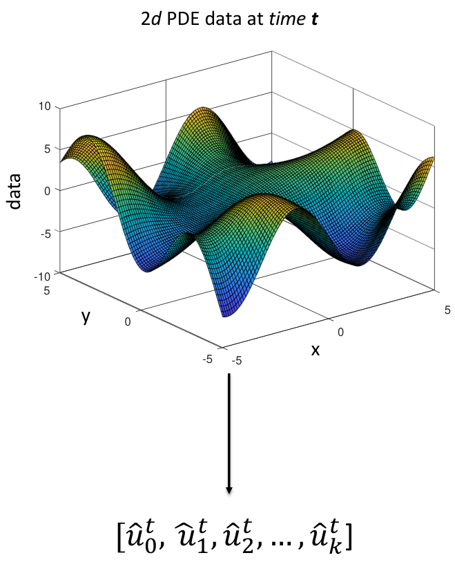
In particular, we use the bidirectional LSTM (hochreiter1997long; graves2005framewise) to better retain the state information from data on grid points which are neighbourhoods in the mesh but far away in input matrix.

The right frame of Figure 3 shows the overall design of the Neural-PDE. Denote the time series data at collocation points as ${\bm{a}}_{1}^{N},{\bm{a}}_{2}^{N},\cdots,{\bm{a}}_{k}^{N}$ with ${\bm{a}}_{i}^{N}=[\hat{u}_{i}^{0},\hat{u}_{i}^{1},\cdots,\hat{u}_{i}^{N}]$ at $i^{th}$ point. The superscript represents different time points. The Neural-PDE takes the past states $\{{\bm{a}}_{1}^{N},{\bm{a}}_{2}^{N},\cdots,{\bm{a}}_{k}^{N}\}$ of all collocation points, and outputs the predicted future states $\{{\bm{b}}_{1}^{M},{\bm{b}}_{2}^{M},\cdots,{\bm{b}}_{k}^{M}\}$, where ${\bm{b}}_{i}^{M}=[v_{i}^{N+1},v_{i}^{N+2},\cdots,v_{i}^{N+M}]$ is the Neural-PDE prediction for the $i^{th}$ collocation point at time points from $N+1$ to $N+M$. The data from time point 0 to $N$ are the training data set.

The Neural-PDE is an encoder-decoder style sequence model that first maps the input data to a low dimensional latent space that

$${\bm{h}}_{i}=\overrightarrow{\mathrm{LSTM}}({\bm{a}}_{i})\oplus\overleftarrow{\mathrm{LSTM}}({\bm{a}}_{i}),$$

(3.2.1)

where $\oplus$ denotes concatenation and ${\bm{h}}_{i}$ is the latent embedding of point ${\bm{a}}_{i}$ under the environment.

One then decoder, another bi-lstm with a dense layer:

$$v_{i}=\left(\overrightarrow{\mathrm{LSTM}}({\bm{h}}_{i})\oplus\overleftarrow{\mathrm{LSTM}}({\bm{h}}_{i})\right)\cdot\mathbf{W},$$

(3.2.2)

where $\mathbf{W}$ is the learnable weight matrix in the dense layer. Moreover, the final decode layers could also have an optional self attention (vaswani2017attention) layer, which makes the model easier to learn long-range dependencies of the mesh grids.

During training process, mean squared error (MSE) loss $\mathcal{L}$ is used as we typically don’t know the specific form of the PDE.

$$\mathcal{L}=\sum_{t=N+1}^{N+M}\sum_{i=1}^{k}||\hat{u}_{i}^{t}-v_{i}^{t}||^{2}~,$$

(3.2.3)

In order to feed the data into our sequence model framework, we map the PDE solution data onto a $K\times N$ matrix, where $K\in\mathbb{Z}^{+}$ is the dimension of the grid points and $N\in\mathbb{Z}^{+}$ is the length of the time series data on each grid point. There is no regularization for the input order of the grid points data in the matrix because of the bi-directional structure of the Neural-PDE. For example, a $2D$ heat equation at some time $t$ is reshaped into a $1D$ vector (See Fig.  2). Then the matrix is formed accordingly.

For a $n$-dimensional time-dependent partial differential equation with $K$ collocation points, the input and output data for $t\in(0,T)$ will be of the form:

		${\bm{A}}(K,N)=\begin{bmatrix}{\bm{a}}_{0}^{N}\\ \vdots\\ {\bm{a}}_{\ell}^{N}\\ \vdots\\ {\bm{a}}_{K}^{N}\\ \end{bmatrix}=\begin{bmatrix}\hat{u}_{0}^{0}&\hat{u}_{0}^{1}&\cdots&\hat{u}_{0}^{n}&\cdots&\hat{u}_{0}^{N}\\ \vdots&\vdots&\ddots&\vdots&\ddots&\vdots\\ \hat{u}_{\ell}^{0}&\hat{u}_{\ell}^{1}&\cdots&\hat{u}_{\ell}^{n}&\cdots&\hat{u}_{\ell}^{N}\\ \vdots&\vdots&\ddots&\vdots&\ddots&\vdots\\ \hat{u}_{K}^{0}&\hat{u}_{K}^{1}&\cdots&\hat{u}_{K}^{n}&\cdots&\hat{u}_{K}^{N}\end{bmatrix}$		(3.3.1)
		${\bm{B}}(K,M)=\begin{bmatrix}{\bm{b}}_{0}^{M}\\ \vdots\\ {\bm{b}}_{\ell}^{M}\\ \vdots\\ {\bm{b}}_{K}^{M}\\ \end{bmatrix}=\begin{bmatrix}v_{0}^{N+1}&v_{0}^{N+2}&\cdots&v_{0}^{N+m}&\cdots&v_{0}^{N+M}\\ \vdots&\vdots&\ddots&\vdots&\ddots&\vdots\\ v_{\ell}^{N+1}&v_{\ell}^{N+2}&\cdots&v_{\ell}^{N+m}&\cdots&v_{k}^{N+M}\\ \vdots&\vdots&\ddots&\vdots&\ddots&\vdots\\ v_{K}^{N+1}&v_{K}^{N+2}&\cdots&v_{K}^{N+m}&\cdots&v_{K}^{N+M}\\ \end{bmatrix}$		(3.3.2)

Here $N=\frac{T}{\delta t}$ and each row $\ell$ represents the time series data at the $\ell^{th}$ mesh grid, and $M$ is the time length of the predicted data.

By adding Bidirectional LSTM encoder in the Neural-PDE, it will automatically extract the information from the time series data as:

$${\bm{B}}(K,M)=PDESolver({\bm{A}}(K,N))=PDESolver({\bm{a}}_{0}^{N},{\bm{a}}_{1}^{N},\cdots\;{\bm{a}}_{i}^{N},\cdots\;,{\bm{a}}_{K}^{N})$$

(3.3.3)

Consider the $1D$ wave equation:

		$\displaystyle u_{tt}=cu_{xx},\;x\in[0,1],\;t\in[0,2]~,$		(4.0.2)
		$\displaystyle u(x,0)=sin(4\pi x)$		(4.0.3)
		$\displaystyle u(0,t)=u(1,t)$		(4.0.4)

Let $c=\frac{1}{16\pi^{2}}$ and use the analytical solution given by the characteristics for the training and testing data:

$$u(x,t)=\frac{1}{2}(sin(4\pi x+t)+sin(4\pi x-t))~.$$

(4.0.5)

Here we used $\delta x=1\times 10^{-2}$, $\delta t=1\times 10^{-2}$, and the mesh grid size is $101$. We obtained a MSE $3.5401\times 10^{-5}$. The test dataset batch size is $25$ and thus the total discrete testing time period is $250$. Figures 4$(a)$ and 4$(b)$ are the heat map for the exact test data and our predicted test data. Figure 4$(c)$ shows both training and cross-validation errors of Neural-PDE convergent within $20$ epochs.

We selected the final four states for computation and compared them with analytic solutions. The result indicates that the Neural-PDE is robust in capturing the physical laws of wave equation and predicting the sequence time period. See Figure 5.

The 1D wave equation case maps the data into a matrix (3.3.1) with its original spatial locations. In this test, we solve the 2D heat equation describing how the motion or diffusion of a heat flow evolves over time. Here the 2-dimensional PDE grid in space is mapped into matrix without regularization of the position. The experimental results show that the Neural-PDE is able to capture the valuable features regardless of the order of the grid points in the matrix. Let’s start with a 2D heat equation as follows:

		$\displaystyle u_{t}=u_{xx}+u_{yy}~,$		(4.0.6)
		$\displaystyle u(x,y,0)=\left\{\begin{array}[]{@{}ll@{}}0.9,&\text{if}\ (x-1)^{2}+(y-1)^{2}<0.25\\ 0.1,&\text{otherwise}\end{array}\right.$
		$\displaystyle\Omega=[0,2]\times[0,2],\;t\in[0,0.15]~.$		(4.0.9)

Figures 6 and 7 show the test of the Neural-PDE using the 2D heat equation. We obtained a MSE $\mathcal{O}(10^{-6})$.

Inviscid Burgers’ equation is a classical nonlinear PDE in fluid dynamics. In this example, we consider a $2D$ invicid Burgers’ equation which has the following hyperbolic form:

		$\displaystyle\frac{\partial u}{\partial t}+u\frac{\partial u}{\partial x}+v\frac{\partial u}{\partial y}=0~,\quad\frac{\partial v}{\partial t}+u\frac{\partial u}{\partial x}+v\frac{\partial u}{\partial y}=0~,$		(4.0.10)
		$\displaystyle\Omega=[0,1]\times[0,1],t\in[0,1]~,$		(4.0.11)

and with the initial and boundary conditions:

		$\displaystyle u(0.25\leq x\leq 0.75,\ 0.25\leq y\leq 0.75,t=0)=0.9~,$		(4.0.12)
		$\displaystyle v(0.25\leq x\leq 0.75,\ 0.25\leq y\leq 0.75,t=0)=0.5~,$		(4.0.13)
		$\displaystyle u(0,y,t)=u(1,y,t)=v(x,0,t)=v(x,1,t)=0~.$		(4.0.14)

The invicid Burgers’ equation is difficult to solve due to the discontinuities (shock waves) in the solutions. We use a upwinding finite difference scheme to create the training data and put the velocity $u,v$ in to the input matrix. Let $\delta x=\delta y=10^{-2},\delta t=10^{-3}$, our empirical results (see Figure 9) show that the Neural-PDE is able to learn the shock waves, boundary conditions and the rules of the equation, and predict $u$ and $v$ simultaneously with an overall MSE of $2.3070\times 10^{-6}$. The heat maps of exact solution and predicted solution are shown in Figure 8.

Finally, let’s consider the following $2D$ Cahn–Hilliard–Navier–Stokes system widely used for modeling complex fluids:

		$\displaystyle{\bm{u}}_{t}+{\bm{u}}\cdot\nabla{\bm{u}}=-\nabla p+\nu\Delta{\bm{u}}-\phi\nabla\mu~,$		(4.0.15)
		$\displaystyle\phi_{t}{}+\nabla\cdot({\bm{u}}\phi)=M\Delta\mu~,$		(4.0.16)
		$\displaystyle\mu=\lambda(-\Delta\phi+\frac{\phi}{\eta^{2}}(\phi^{2}-1))~,$		(4.0.17)
		$\displaystyle\nabla\cdot{\bm{u}}=0~.$		(4.0.18)

In this example we use the following initial condition:

	$\displaystyle\phi(x,y,0)$	$\displaystyle=(\frac{1}{2}-50\tanh(f_{1}-0.1))+(\frac{1}{2}-50\tanh(f_{2}-0.1))~,~{\rm where}$		(4.0.19)
	$\displaystyle f_{1}(x,y)$	$\displaystyle=\sqrt{(x+0.12)^{2}+(y)^{2}},\;f_{2}(x,y)=\sqrt{(x-0.12)^{2}+(y)^{2}}~$		(4.0.20)
	$\displaystyle\text{with}\;x$	$\displaystyle\in[-0.5,0.5],\;y\in[-0.5,0.5],\;t\in[0,1],\;M=0.1,\;\nu=0.01,\;\eta=0.1.$		(4.0.21)

This fluid system can be derived by the energetic variational approach (forster2013mathematical). Here ${\bm{u}}$ is the velocity and $\phi(x,y,t)\in[0,1]$ is the labeling function of the fluid phase. $M$ is the diffusion coefficient, and $\mu$ is the chemical potential of $\phi$. Equation (4.0.18) indicates the incompressibility of the fluid. Solving such PDE system is notorious because of its high nonlinearity and multi-physical and coupled features. A challenge of deep learning in solving a system like this is how to process the data to improve the learning efficiency when the input matrix consists of variables such as $\phi\in[0,1]$ with large magnitude value and variable of very small values such as $p\sim 10^{-5}$. For the Neural-PDE to better extract and learn the physical features of variables in different spatial-temporal scales, we normalized the $p$ data with a $sigmoid$ function. We set $\delta t=5\times 10^{-4}$. Here the training dataset is generated by the FEM solver FreeFem++ (MR3043640) using a Crank-Nicolson in time $C^{0}$ finite element scheme. Our Neural-PDE prediction shows that the physical features of $p$ and $\phi$ have been successfully captured with an overall MSE: $6.1631\times 10^{-7}$ (see Figure 10). In this example, we only coupled $p$ and $\phi$ together to show the learning ability of the Neural-PDE. Another approach is to couple $p$, $\phi$ and the velocity ${\bm{u}}$ together in the training data to predict all the related variables ($p,\phi,{\bm{u}}$), which would need more normalization and regularization, techniques such as batch normalization would be helpful, please see recent research on PINN based neural network in solving such system (wight2020solving).

References

- (1) R. Courant, K. Friedrichs, H. Lewy, On the partial difference equations of mathematical physics, IBM journal of Research and Development 11 (2) (1967) 215–234.
- (2) S. Osher, J. A. Sethian, Fronts propagating with curvature-dependent speed: algorithms based on hamilton-jacobi formulations, Journal of computational physics 79 (1) (1988) 12–49.
- (3) R. J. LeVeque, Numerical methods for conservation laws, Vol. 3, Springer, 1992.
- (4) B. Cockburn, G. E. Karniadakis, C.-W. Shu, Discontinuous Galerkin methods: theory, computation and applications, Vol. 11, Springer Science & Business Media, 2012.
- (5) J. W. Thomas, Numerical partial differential equations: finite difference methods, Vol. 22, Springer Science & Business Media, 2013.
- (6) C. Johnson, Numerical solution of partial differential equations by the finite element method, Courier Corporation, 2012.
- (7) G. C. Peng, M. Alber, A. B. Tepole, W. R. Cannon, S. De, S. Dura-Bernal, K. Garikipati, G. Karniadakis, W. W. Lytton, P. Perdikaris, et al., Multiscale modeling meets machine learning: What can we learn?, Archives of Computational Methods in Engineering (2020) 1–21.
- (8) G. Litjens, T. Kooi, B. E. Bejnordi, A. A. A. Setio, F. Ciompi, M. Ghafoorian, J. A. Van Der Laak, B. Van Ginneken, C. I. Sánchez, A survey on deep learning in medical image analysis, Medical image analysis 42 (2017) 60–88.
- (9) J. Devlin, M.-W. Chang, K. Lee, K. Toutanova, Bert: Pre-training of deep bidirectional transformers for language understanding, arXiv preprint arXiv:1810.04805 (2018).
- (10) Y. LeCun, L. Bottou, Y. Bengio, P. Haffner, Gradient-based learning applied to document recognition, Proceedings of the IEEE 86 (11) (1998) 2278–2324.
- (11) A. Krizhevsky, I. Sutskever, G. E. Hinton, Imagenet classification with deep convolutional neural networks, in: Advances in neural information processing systems, 2012, pp. 1097–1105.
- (12) G. Hinton, L. Deng, D. Yu, G. E. Dahl, A.-r. Mohamed, N. Jaitly, A. Senior, V. Vanhoucke, P. Nguyen, T. N. Sainath, et al., Deep neural networks for acoustic modeling in speech recognition: The shared views of four research groups, IEEE Signal processing magazine 29 (6) (2012) 82–97.
- (13) J. Han, A. Jentzen, E. Weinan, Solving high-dimensional partial differential equations using deep learning, Proceedings of the National Academy of Sciences 115 (2018) 8505 – 8510.
- (14) Z. Long, Y. Lu, X. Ma, B. Dong, Pde-net: Learning pdes from data, in: International Conference on Machine Learning, 2018, pp. 3208–3216.
- (15) J. Sirignano, K. Spiliopoulos, Dgm: A deep learning algorithm for solving partial differential equations, Journal of computational physics 375 (2018) 1339–1364.
- (16) M. Raissi, P. Perdikaris, G. E. Karniadakis, Physics-informed neural networks: A deep learning framework for solving forward and inverse problems involving nonlinear partial differential equations, Journal of Computational Physics 378 (2019) 686–707.
- (17) A. Sherstinsky, Fundamentals of recurrent neural network (rnn) and long short-term memory (lstm) network, Physica D: Nonlinear Phenomena 404 (2020) 132306.
- (18) U. M. Ascher, S. J. Ruuth, R. J. Spiteri, Implicit-explicit runge-kutta methods for time-dependent partial differential equations, Applied Numerical Mathematics 25 (2-3) (1997) 151–167.
- (19) R. T. Chen, Y. Rubanova, J. Bettencourt, D. K. Duvenaud, Neural ordinary differential equations, in: Advances in neural information processing systems, 2018, pp. 6571–6583.
- (20) Z. Huang, W. Xu, K. Yu, Bidirectional lstm-crf models for sequence tagging, arXiv preprint arXiv:1508.01991 (2015).
- (21) M. Schuster, K. K. Paliwal, Bidirectional recurrent neural networks, IEEE transactions on Signal Processing 45 (11) (1997) 2673–2681.
- (22) S. Hochreiter, J. Schmidhuber, Long short-term memory, Neural computation 9 (8) (1997) 1735–1780.
- (23) Z. C. Lipton, J. Berkowitz, C. Elkan, A critical review of recurrent neural networks for sequence learning, arXiv preprint arXiv:1506.00019 (2015).
- (24) A. Graves, J. Schmidhuber, Framewise phoneme classification with bidirectional lstm and other neural network architectures, Neural networks 18 (5-6) (2005) 602–610.
- (25) T. Mikolov, S. Kombrink, L. Burget, J. Černockỳ, S. Khudanpur, Extensions of recurrent neural network language model, in: 2011 IEEE international conference on acoustics, speech and signal processing (ICASSP), IEEE, 2011, pp. 5528–5531.
- (26) Y. Lu, A. Zhong, Q. Li, B. Dong, Beyond finite layer neural networks: Bridging deep architectures and numerical differential equations, in: International Conference on Machine Learning, 2018, pp. 3276–3285.
- (27) A. Vaswani, N. Shazeer, N. Parmar, J. Uszkoreit, L. Jones, A. N. Gomez, Ł. Kaiser, I. Polosukhin, Attention is all you need, in: Advances in neural information processing systems, 2017, pp. 5998–6008.
- (28) J. Forster, Mathematical modeling of complex fluids, Master’s, University of Wurzburg (2013).
- (29)
F. Hecht, New development in freefem++, J. Numer.
Math. 20 (3-4) (2012) 251–265.
URL https://freefem.org/ - (30) C. L. Wight, J. Zhao, Solving allen-cahn and cahn-hilliard equations using the adaptive physics informed neural networks, arXiv preprint arXiv:2007.04542 (2020).