Quantum Computation of Finite-Temperature Static and Dynamical Properties of Spin Systems Using Quantum Imaginary Time Evolution

The QITE algorithm is carried out by iterating the procedure of constructing the circuit from the QITE unitaries obtained at the previous imaginary time steps, measuring the operators in eq. 10, constructing the linear system in eq. 5, solving for $\bm{x[l]}$, and propagating the state with the new unitary $e^{-i\Delta\tau\hat{G}[l]}$.

Finite-temperature static observables have been previously computed on quantum hardware using the QMETTS algorithm by averaging over the observable evaluated from each METTS sample state Motta et al. 2019. In this work, we show that finite-temperature dynamical observables, in particular finite-temperature dynamical correlation functions, can be computed using a similar averaging procedure as for finite-temperature static observables.

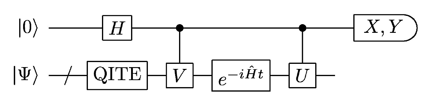
Measuring $X$ ($Y$) on the ancilla yields the real (imaginary) part of the dynamical correlation function on a single QITE-evolved basis state:

If the initial states are the METTS sample states, an unweighted average over the initial states yields the finite-temperature dynamical correlation function $\expectationvalue{U(t)V}_{\beta}$. In this work, we consider trace evaluation in the exact expression of an observable $\hat{O}$ at finite temperature:

The numerator trace and the denominator trace are either evaluated by full sampling over the entire Hilbert space, denoted as full trace evaluation, or by random sampling over a subspace of the Hilbert space, denoted as stochastic trace evaluation. If $\hat{O}=U(t)V$, eq. 16 yields the finite-temperature dynamical correlation function $\expectationvalue{U(t)V}_{\beta}$. $\hat{O}$ can also be a static observable, in which case eq. 16 yields the static observable at finite temperature.

If we include all $4^{D}$ Pauli strings over each domain consisting of $D$ qubits, each QITE unitary $e^{-i\Delta\tau\hat{G}[l]}$ applied as in eq. 4 yields $\mathcal{O}(N4^{D})$ multi-qubit rotation gates by the standard rotation gate decomposition Nielsen and Chuang 2019, which results in a circuit too deep on near-term quantum devices even for $D=2$. Because of this prohibitive resource overhead, we describe a systematic method to reduce the number of Pauli strings in the QITE unitaries when the Hamiltonian and initial state have $\mathbb{Z}_{2}$ symmetries.

$\mathbb{Z}_{2}$ symmetries on qubit Hamiltonians have direct parallels with the stabilizer formalism in quantum error-correcting codes Gottesman 1998. Suppose the Hamiltonian has $d$ $\mathbb{Z}_{2}$ symmetries, i.e. $\hat{H}$ commutes with elements of a group isomorphic to $\mathbb{Z}_{2}^{d}$ generated independently by $d$ Pauli strings, and the initial state is in the +1 eigenspace of all $d$ generators. If we regard the symmetry group $\mathbb{Z}_{2}^{d}$ as the stabilizer $\mathcal{S}$, the symmetry sector of the initial state corresponds to the stabilizer subspace $V_{\mathcal{S}}$.

In stabilizer codes, the normalizer of the stabilizer $\mathcal{N}(\mathcal{S})$ includes all Pauli strings that commute with elements of the stabilizer $\mathcal{S}$, and all valid operations on the code space are in the quotient group $\mathcal{N}(\mathcal{S})/\mathcal{S}$. Intuitively, to preserve $\mathbb{Z}_{2}$ symmetries, among all Pauli strings from $\mathcal{P}_{\hat{H}[l]}$ the QITE unitaries should only include those from the quotient group $\mathcal{N}(\mathcal{S})/\mathcal{S}$. We now show that the original QITE algorithm subsumes the requirement that the Pauli strings should be chosen from $\mathcal{N}(\mathcal{S})/\mathcal{S}$ because the action of the unitary $e^{-i\Delta\tau\hat{G}[l]}$ with the Pauli strings from the unreduced set $\mathcal{P}_{\hat{H}[l]}$ is the same as the action with Pauli strings from the reduced set $\mathcal{P}_{\hat{H}[l]}\cap\mathcal{N}(\mathcal{S})/\mathcal{S}$. This result is stated as the following proposition, proved and discussed in appendix A.

Further reduction in the number of Pauli strings can be achieved by recalling from Ref. Motta et al. 2019 that when the Hamiltonian and the initial state are real in the computational basis, the state after imaginary time evolution must be real. Thus, only Pauli strings with an odd number ofw $Y$ need to be included in the QITE unitaries. Since $\mathbb{Z}_{2}$ symmetries and the conditions of a real Hamiltonian and initial state are independent, when both conditions are satisfied, the number of Pauli strings can be reduced using both conditions, in which case the reduced set of Pauli strings is modified to $\mathcal{P}_{\hat{H}[l]}\cap\mathcal{N}(\mathcal{S})/\mathcal{S}\cap\{\sigma_{\bm{\mu}}:\sum_{j}\delta_{\mu_{j},y}\equiv 1\text{ (mod 2)}\}$.

In practice the Proposition is used inductively on the Trotter terms $\hat{H}[l]$, which implies the stabilizer need to be chosen such that every element of the stabilizer commutes with all $\hat{H}[l]$, or equivalently with $\hat{H}$. For spin Hamiltonians, the stabilizer generators are usually global $\mathbb{Z}_{2}$ symmetries such as $Z^{\otimes N}$ and $X^{\otimes N}$. For general Hamiltonians, the $\mathbb{Z}_{2}$ symmetries can be found by Gaussian elimination on the parity check matrix formed from the Hamiltonian terms Bravyi et al..

Even with reduction of Pauli strings in the QITE unitaries by $\mathbb{Z}_{2}$ symmetries, applying the QITE unitaries as in eq. 4 may still result in a circuit too deep to be implemented on current quantum hardware. In this section we describe circuit optimization techniques that further reduce circuit depth.

In two-site calculations, both the QITE circuit and the real time evolution circuit can be optimized to constant depth with a standard one- and two-qubit gate set, regardless of the number of imaginary and real time steps. For example, in two-site TFIM there is only one Pauli string $X_{0}Y_{1}$ in the QITE unitaries after reduction by the $\mathbb{Z}_{2}$ symmetry $Z_{0}Z_{1}$. Suppose the unitary applied to the state at the $k$-th imaginary time step is $e^{-i\Delta\tau x_{k}X_{0}Y_{1}}$. Then the unitaries at all imaginary time steps can be multiplied into a single two-qubit rotation gate $e^{-i\theta X_{0}Y_{1}/2}$ where $\theta=2\Delta\tau\sum_{k}x_{k}$. For real time evolution, the two-qubit operator $e^{-i\hat{H}t}$ is decomposed by the $KAK$ decomposition Khaneja et al. 2001; Kraus and Cirac 2001; Vatan and Williams 2004; Vidal and Dawson 2004 into six single-qubit gates and two CNOT gates.

Since the QITE unitaries are real, we use the one-parameter single-qubit gate $R_{y}(\theta)=U_{3}(\theta,0,0)$ in the recompiled circuit for QITE, while for real time evolution we keep the $U_{3}$ gate as the parametrized single-qubit gate.

To mitigate the effect of hardware noise on the measurement results, we post-process our hardware data by error mitigation methods including post-selection, readout error mitigation and phase-and-scale correction. Post-selection and readout error mitigation are applied to the measurement outcomes at each imaginary time step in the QITE subroutine; phase-and-scale correction is applied to the final computed finite-temperature dynamical correlation function as a single-step post-processing.

Post-selection is performed on $\mathbb{Z}_{2}$ symmetries discussed in section III.1. When the Hamiltonian and the initial state have $\mathbb{Z}_{2}$ symmetries, the final state after imaginary or real time evolution should have the same stabilizer parities as the initial state. However, during execution of the circuit, gate errors and qubit decoherence can induce nonzero overlap of the qubit state with the subspace of the wrong parity. Post-selection can mitigate these undesirable effects by discarding measurement outcomes with the wrong parity Bonet-Monroig et al. 2018; McArdle et al. 2019b.

We specifically consider the symmetry from a single stabilizer generator. If the operator to be measured is an ancilla operator, we can simply measure the stabilizer generator on all the system qubits and read off the parity without interfering with measurement of the ancilla. If the operator to be measured acts on system qubits, we need to simultaneously measure the operator and the stabilizer generator, which is possible because all operators in eq. 10 commute with the stabilizer generator by our choice of Pauli strings in the QITE unitaries in section III.1. Specifically, each operator and the stabilizer generator can be simultaneously measured by using Clifford gates to transform the Pauli string components of the operator and the stabilizer generator until they are qubit-wise commuting, so that their expectation values can be read off on different qubits Gokhale et al.; Crawford et al.; Yen et al. 2020; Hamamura and Imamichi 2020.

Figure 4 shows the circuit to simultaneously measure the stabilizer generator $Z_{0}Z_{1}Z_{2}Z_{3}$ and a Pauli string that commutes with it in a four-site QITE calculation. The sequence of CNOT gates after the QITE circuit in fig. 4 transforms $Z_{0}Z_{1}Z_{2}Z_{3}$ to $Z_{3}$. Since $Z_{3}$ acts on a single qubit, it necessarily qubit-wise commutes with the transformed Pauli string. In practice, we stop applying CNOT gates when the transformed Pauli string becomes qubit-wise commuting with the transformed stabilizer generator, and therefore the number of CNOT gates added to the end of the circuit ranges from zero to three.

To account for noise in the final measurement, the built-in readout error mitigation routine in Qiskit Asfaw et al. is applied to each measurement outcome. Because of the small size of the systems we study, for $N$ qubits we carry out full calibration on all $2^{N}$ initial states. Application of the inverse of the calibration matrix to the raw measurement counts is performed by the default least-square fitting method.

We assess the effectiveness of applying post-selection and readout error mitigation at every imaginary step of QITE by simulating the finite-temperature energies of two-site and four-site TFIMs using full trace evaluation with measurement sampling and the noise model from ibmq_rome. In both panels of fig. 5, QITE is applied with Pauli strings reduced and circuits optimized. In particular, four-site QITE unitaries are of domain size $D=2$ and recompiled with three rounds of gates. From fig. 5 we can see that both readout error mitigation and post-selection shift the raw data toward the exact data, confirming the effectiveness of both schemes in reducing the effect of noise. Furthermore, a combination of readout error mitigation and post-selection is observed to be most effective in mitigating the errors, which is not apparent on two sites in fig. 5 presumably because of the small size of the system but clearly evident on four sites in fig. 5.

In calculations of finite-temperature dynamical correlation functions, the ancilla qubit is in the state $\ket{+}$ before entangling with the system qubits. When there is a long sequence of gates in the real time propagator $e^{-i\hat{H}t}$, decoherence of the ancilla qubit such as amplitude damping to the qubit ground state $\ket{0}$ and depolarization will significantly affect the $X$ and $Y$ measurement results on the ancilla. To mitigate the effect of ancilla decoherence, we apply phase-and-scale correction Chiesa et al. 2019; Francis et al. 2020 as a single-step post-processing to the result at the end of the calculation. The only finite-temperature dynamical correlation function considered in this work is $\expectationvalue{Z_0(t)Z_0}_{\beta}$, which is equal to 1 analytically at $t=0$. Hence, we apply phase-and-scale correction by dividing the raw hardware $\expectationvalue{Z_0(t)Z_0}_{\beta}$ at each $t$ by the raw hardware $\expectationvalue{Z_0(t=0)Z_0}_{\beta}$ to enforce the condition $\expectationvalue{Z_0(t=0)Z_0}_{\beta}=1$.

We study the two-site TFIM defined in eq. 17 by setting $h=1$ and varying $J$. The finite-temperature energy $\expectationvalue{E}_{\beta}$ and static correlation function $\expectationvalue{X_0X_1}_{\beta}$ are calculated on the Hamiltonians with $J=\pm 1,\pm 3$, while the finite-temperature dynamical correlation function $\expectationvalue{Z_0(t)Z_0}_{\beta}$ and excitation spectra are calculated on the Hamiltonian with $J=3$. In all calculations, finite-temperature observables are calculated by full trace evaluation and the circuits are optimized according to the circuit optimization procedures in section III.2.

Figure 6 shows the finite-temperature energy $\expectationvalue{E}_{\beta}$ and static correlation function $\expectationvalue{X_0X_1}_{\beta}$ of the two-site TFIM with $J=\pm 1,\pm 3$ from $\beta=0$ to $\beta=2$. In both fig. 6 and fig. 6 the finite-temperature observables obtained on hardware are in good agreement with exact values. Further, if we regard each finite-temperature variable as a function of $J$, analytically it can be shown that $\expectationvalue{E}_{\beta}(J)=\expectationvalue{E}_{\beta}(-J)$ and $\expectationvalue{X_0X_1}_{\beta}(J)=-\expectationvalue{X_0X_1}_{\beta}(-J)$. This relation is satisfied in the hardware data. In each of the observables we calculated, the mean absolute percentage error between hardware and exact results averaged over all $\beta$ ranges from 1% to 4%.

Next, finite-temperature dynamical properties were calculated on the two-site TFIM with $J=3,h=1$. The dynamical correlation function $\expectationvalue{Z_0(t)Z_0}_{\beta}$ is evaluated from $\beta=0$ to $\beta=2$ and at real time from $t=0$ to $t=8\pi$. Figures 7 and 7 show the real and imaginary parts of $\expectationvalue{Z_0(t)Z_0}_{\beta}$ at $\beta=0.2$ and $\beta=1.8$ up to $t=4\pi$. From figs. 7 and 7 we see that even without phase-and-scale correction, the real and imaginary parts of $\expectationvalue{Z_0(t)Z_0}_{\beta}$ agree well with the exact results at both small and large $\beta$, presumably due to the constant and shallow depth of the real time evolution circuit.

In fig. 7 we plot the excitation spectra of the two-site TFIM at $\beta=0.2$. The exact excitation spectrum is obtained by a Fourier transform of the exact $\expectationvalue{Z_0(t)Z_0}_{\beta}$ at the same points in real time as the $\expectationvalue{Z_0(t)Z_0}_{\beta}$ obtained on hardware. From the plot, we can see that the hardware excitation spectrum agrees well with the exact

To analyze the evolution of the excitation spectra across different temperatures, we plot the amplitudes at the two emission frequencies versus $\beta$ in fig. 7. Analytically, the amplitude of the transition from an initial state $\ket{\Psi_i}$ to a final state $\ket{\Psi_f}$ is $e^{-\beta E_{f}}|\langle\Psi_{i}|Z_{0}|\Psi_{f}\rangle|^{2}/\mathcal{Z}$, where $E_{f}$ is the energy of the final state and $\mathcal{Z}$ is the partition function. In the two-site TFIM, the only allowed transitions are between the two states in each of the two-dimensional eigenspaces of $Z_{0}Z_{1}$ with eigenvalues $\pm 1$. The frequency $\pm 7.18$ corresponds to a transition in the $+1$ eigenspace, where the ground state lies, and the frequency $\pm 5.94$ corresponds to a transition in the $-1$ eigenspace, where the first excited state lies. As the temperature decreases from infinite temperature ($\beta$ increases from 0), the populations in the two lowest states first increase until the ground state population dominates over that of the first excited state at around $\beta=0.4$, a trend reproduced by the amplitudes obtained from hardware data in fig. 7. Thus, fig. 7 shows that quantum hardware accurately captures the finite-temperature dynamics of the two-site TFIM across a wide range of temperatures.

We next proceed to four-site spin systems. We study the four-site TFIM defined in eq. 17 with $J=3,h=1$. Full trace evaluation is employed unless otherwise specified.

First, let us consider the gate count in the four-site circuits. For the four-site TFIM with $D=2$, after reduction by the $\mathbb{Z}_{2}$ symmetry $Z_{0}Z_{1}Z_{2}Z_{3}$ there are six weight-two Pauli strings, which are the ones given in eq. 19. If we Trotterize the QITE unitaries as in eq. 4, each unitary requires 12 CNOT gates by the standard rotation gate decomposition Nielsen and Chuang 2019, which becomes unfeasible on near-term quantum hardware after the first few imaginary time steps. When $D=4$, even after reduction by one $\mathbb{Z}_{2}$ symmetry there are still 28 Pauli strings in each QITE unitary. After Trotterization and rotation gate decomposition, each QITE unitary requires more than 50 CNOT gates for a single imaginary time step. Hence, when $D=2$, we compute finite-temperature observables both by Trotterizing and by recompiling the QITE unitaries with three gate rounds; when $D=4$, we only recompile the QITE unitaries with three gate rounds. To obtain dynamical correlation functions, we additionally recompile the real time propagator $e^{-i\hat{H}t}$ with five gate rounds. The number of gate rounds is chosen so that the fidelity in eq. 22 is at least 0.999 on average in each calculation.

Figure 8 shows the finite-temperature energy $\expectationvalue{E}_{\beta}$ and static correlation functions $\expectationvalue{X_0X_1}_{\beta},\expectationvalue{X_0X_2}_{\beta},\expectationvalue{X_0X_3}_{\beta}$ of the four-site TFIM. From the figure, we can see that the finite-temperature observables calculated with Trotterized $D=2$ QITE unitaries deviate from those calculated with $D=2$ recompiled QITE unitaries or $D=4$ recompiled QITE unitaries after $\beta=0.1$. This deviation is due to the deep circuit resulting from 12 layers of CNOT gates per imaginary time step, compared to 3 layers of CNOT gates per imaginary time step in the recompiled circuit. Moreover, even the recompiled QITE unitaries are not able to track the exact finite-temperature observables after the first few $\beta$. In particular, the slope is reversed compared to the exact result after $\beta=0.5$. QITE up to $\beta=0.5$ corresponds to 5 imaginary time steps and hence 15 layers of CNOT gates, which is almost at the limit of circuit depth on these quantum devices.

We examine more closely the calculations with recompiled QITE unitaries and focus on the data at $\beta\leq 0.5$. For both $D=2$ and $D=4$, the recompiled QITE unitaries apply the same number of layers of gates at each imaginary time step, so the difference in calculated observables is formally caused by the difference in domain sizes. Since the domain size should grow with correlation length and hence with imaginary time Motta et al. 2019, we should expect the hardware results to be closer to the exact results with $D=4$ than with $D=2$ especially at large $\beta$. However, this hypothesis only holds for $\expectationvalue{X_0X_2}_{\beta}$ and $\expectationvalue{X_0X_3}_{\beta}$ but not for $\expectationvalue{E}_{\beta}$ and $\expectationvalue{X_0X_1}_{\beta}$. Failure of this hypothesis is likely due to that fact that the larger 28-dimensional linear system arising from $D=4$ incorporates more errors from hardware noise compared to the smaller 6-dimensional linear system arising from $D=2$.

To explore the scalability of our method, we compare stochastic trace evaluation with full trace evaluation in calculating the finite-temperature energy of the four-site TFIM. Stochastic trace evaluation is performed by uniformly selecting initial states in the full trace evaluation result with recompiled $D=2$ QITE unitaries. In fig. 9, we plot the stochastic trace evaluation results with 10 and 20 samples along with the full trace evaluation and exact results; the inset shows the running average of $\expectationvalue{E}_{\beta}$ versus number of samples $n_{\text{samples}}$. As can be seen from the figure, random sampling with 10 samples already reproduced the results from full sampling on all 16 initial states, indicating that using scalable sampling schemes is a promising approach to studying larger systems.

Finally, in fig. 10 we show the dynamical properties of the four-site TFIM with $J=3,h=1$ at $\beta=0.2$. The calculation is implemented by recompiling $D=2$ QITE unitaries with three gate rounds and real time propagation with five gate rounds. Figure 10 shows the real and imaginary parts of $\expectationvalue{Z_0(t)Z_0}_{\beta}$ after phase-and-scale correction. With this correction, both the real and the imaginary parts show good agreement with the exact result. Figure 10 shows the excitation spectra obtained by Fourier transforming the exact and phase-and-scale-corrected hardware $\expectationvalue{Z_0(t)Z_0}_{\beta}$ at the same points in real time. The excitation spectrum from hardware data accurately reproduces not only the frequencies $\omega=0,\pm 4.90,\pm 6.37,7.84$ but also the peak amplitudes.

The favorable agreement of the hardware $\expectationvalue{Z_0(t)Z_0}_{\beta}$ with the exact result is in contrast with the deviation of finite-temperature static observables from the exact results in fig. 8. In fact, the raw hardware $\expectationvalue{Z_0(t)Z_0}_{\beta}$ at $t=0$ is $0.821+0.397i$, which is far from the exact value 1, indicating that phase-and-scale correction has a significant effect in correcting raw hardware data. Even though phase does not enter the static observables we computed, lack of a scale correction scheme for the static observables may explain their large deviation from the exact values compared to dynamical observables. More-

References

- Feynman (1982) R. P. Feynman, Simulating physics with computers, Int. J. Theor. Phys. 21, 467 (1982).
- Lloyd (1996) S. Lloyd, Universal Quantum Simulators, Science 273, 1073 (1996).
- Georgescu et al. (2014) I. M. Georgescu, S. Ashhab, and F. Nori, Quantum simulation, Rev. Mod. Phys. 86, 153 (2014).
- Peruzzo et al. (2014) A. Peruzzo, J. McClean, P. Shadbolt, M.-H. Yung, X.-Q. Zhou, P. J. Love, A. Aspuru-Guzik, and J. L. O’Brien, A variational eigenvalue solver on a photonic quantum processor, Nat. Commun. 5, 4213 (2014).
- O’Malley et al. (2016) P. J. J. O’Malley, R. Babbush, I. D. Kivlichan, J. Romero, J. R. McClean, R. Barends, J. Kelly, P. Roushan, A. Tranter, N. Ding, B. Campbell, Y. Chen, Z. Chen, B. Chiaro, A. Dunsworth, A. G. Fowler, E. Jeffrey, E. Lucero, A. Megrant, J. Y. Mutus, M. Neeley, C. Neill, C. Quintana, D. Sank, A. Vainsencher, J. Wenner, T. C. White, P. V. Coveney, P. J. Love, H. Neven, A. Aspuru-Guzik, and J. M. Martinis, Scalable Quantum Simulation of Molecular Energies, Phys. Rev. X 6, 031007 (2016).
- Kandala et al. (2017) A. Kandala, A. Mezzacapo, K. Temme, M. Takita, M. Brink, J. M. Chow, and J. M. Gambetta, Hardware-efficient variational quantum eigensolver for small molecules and quantum magnets, Nature 549, 242 (2017).
- Colless et al. (2018) J. Colless, V. Ramasesh, D. Dahlen, M. Blok, M. Kimchi-Schwartz, J. McClean, J. Carter, W. de Jong, and I. Siddiqi, Computation of Molecular Spectra on a Quantum Processor with an Error-Resilient Algorithm, Phys. Rev. X 8, 011021 (2018).
- Kandala et al. (2019) A. Kandala, K. Temme, A. D. Córcoles, A. Mezzacapo, J. M. Chow, and J. M. Gambetta, Error mitigation extends the computational reach of a noisy quantum processor, Nature 567, 491 (2019).
- Ma et al. (2020) H. Ma, M. Govoni, and G. Galli, Quantum simulations of materials on near-term quantum computers, npj Computational Materials 6, 85 (2020).
- Arute et al. (2020) F. Arute, K. Arya, R. Babbush, D. Bacon, J. C. Bardin, R. Barends, S. Boixo, M. Broughton, B. B. Buckley, D. A. Buell, B. Burkett, N. Bushnell, Y. Chen, Z. Chen, B. Chiaro, R. Collins, W. Courtney, S. Demura, A. Dunsworth, D. Eppens, E. Farhi, A. Fowler, B. Foxen, C. Gidney, M. Giustina, R. Graff, S. Habegger, M. P. Harrigan, A. Ho, S. Hong, T. Huang, W. J. Huggins, L. Ioffe, S. V. Isakov, E. Jeffrey, Z. Jiang, C. Jones, D. Kafri, K. Kechedzhi, J. Kelly, S. Kim, P. V. Klimov, A. Korotkov, F. Kostritsa, D. Landhuis, P. Laptev, M. Lindmark, E. Lucero, O. Martin, J. M. Martinis, J. R. McClean, M. McEwen, A. Megrant, X. Mi, M. Mohseni, W. Mruczkiewicz, J. Mutus, O. Naaman, M. Neeley, C. Neill, H. Neven, M. Y. Niu, T. E. O’Brien, E. Ostby, A. Petukhov, H. Putterman, C. Quintana, P. Roushan, N. C. Rubin, D. Sank, K. J. Satzinger, V. Smelyanskiy, D. Strain, K. J. Sung, M. Szalay, T. Y. Takeshita, A. Vainsencher, T. White, N. Wiebe, Z. J. Yao, P. Yeh, and A. Zalcman, Hartree-Fock on a superconducting qubit quantum computer, Science 369, 1084 (2020).
- Islam et al. (2013) R. Islam, C. Senko, W. C. Campbell, S. Korenblit, J. Smith, A. Lee, E. E. Edwards, C.-C. J. Wang, J. K. Freericks, and C. Monroe, Emergence and Frustration of Magnetism with Variable-Range Interactions in a Quantum Simulator, Science 340, 583 (2013).
- Zhang et al. (2017) J. Zhang, G. Pagano, P. W. Hess, A. Kyprianidis, P. Becker, H. Kaplan, A. V. Gorshkov, Z.-X. Gong, and C. Monroe, Observation of a many-body dynamical phase transition with a 53-qubit quantum simulator, Nature 551, 601 (2017).
- Smith et al. (2019) A. Smith, M. S. Kim, F. Pollmann, and J. Knolle, Simulating quantum many-body dynamics on a current digital quantum computer, npj Quantum Inf. 5, 106 (2019).
- Chiesa et al. (2019) A. Chiesa, F. Tacchino, M. Grossi, P. Santini, I. Tavernelli, D. Gerace, and S. Carretta, Quantum hardware simulating four-dimensional inelastic neutron scattering, Nat. Phys. 15, 455 (2019).
- Francis et al. (2020) A. Francis, J. K. Freericks, and A. F. Kemper, Quantum computation of magnon spectra, Phys. Rev. B 101, 014411 (2020).
- (16) B. Bauer, S. Bravyi, M. Motta, and G. K.-L. Chan, Quantum algorithms for quantum chemistry and quantum materials science, arXiv:2001.03685 .
- Terhal and DiVincenzo (2000) B. M. Terhal and D. P. DiVincenzo, Problem of equilibration and the computation of correlation functions on a quantum computer, Phys. Rev. A 61, 022301 (2000).
- Poulin and Wocjan (2009) D. Poulin and P. Wocjan, Sampling from the Thermal Quantum Gibbs State and Evaluating Partition Functions with a Quantum Computer, Phys. Rev. Lett. 103, 220502 (2009).
- Riera et al. (2012) A. Riera, C. Gogolin, and J. Eisert, Thermalization in nature and on a quantum computer, Phys. Rev. Lett. 108, 080402 (2012).
- Temme et al. (2011) K. Temme, T. J. Osborne, K. G. Vollbrecht, D. Poulin, and F. Verstraete, Quantum Metropolis sampling, Nature 471, 87 (2011).
- Yung and Aspuru-Guzik (2012) M.-H. Yung and A. Aspuru-Guzik, A quantum–quantum Metropolis algorithm, Proc. Natl. Acad. Sci. 109, 754 (2012).
- Martyn and Swingle (2019) J. Martyn and B. Swingle, Product spectrum ansatz and the simplicity of thermal states, Phys. Rev. A 100, 032107 (2019).
- Wu and Hsieh (2019) J. Wu and T. H. Hsieh, Variational Thermal Quantum Simulation via Thermofield Double States, Phys. Rev. Lett. 123, 220502 (2019).
- (24) J.-G. Liu, L. Mao, P. Zhang, and L. Wang, Solving Quantum Statistical Mechanics with Variational Autoregressive Networks and Quantum Circuits, arXiv:1912.11381 .
- (25) G. Verdon, J. Marks, S. Nanda, S. Leichenauer, and J. Hidary, Quantum Hamiltonian-Based Models and the Variational Quantum Thermalizer Algorithm, arXiv:1910.02071 .
- (26) A. N. Chowdhury, G. H. Low, and N. Wiebe, A Variational Quantum Algorithm for Preparing Quantum Gibbs States, arXiv:2002.00055 .
- Zoufal et al. (2020) C. Zoufal, A. Lucchi, and S. Woerner, Variational Quantum Boltzmann Machines (2020), arXiv:2006.06004 .
- Wang et al. (2020) Y. Wang, G. Li, and X. Wang, Variational quantum Gibbs state preparation with a truncated Taylor series (2020), arXiv:2005.08797 .
- Cohn et al. (2020) J. Cohn, F. Yang, K. Najafi, B. Jones, and J. K. Freericks, Minimal effective Gibbs ansatz: A simple protocol for extracting an accurate thermal representation for quantum simulation, Phys. Rev. A 102, 022622 (2020).
- Motta et al. (2019) M. Motta, C. Sun, A. T. K. Tan, M. J. O’Rourke, E. Ye, A. J. Minnich, F. G. S. L. Brandão, and G. K.-L. Chan, Determining eigenstates and thermal states on a quantum computer using quantum imaginary time evolution, Nat. Phys. 10.1038/s41567-019-0704-4 (2019).
- McArdle et al. (2019a) S. McArdle, T. Jones, S. Endo, Y. Li, S. C. Benjamin, and X. Yuan, Variational ansatz-based quantum simulation of imaginary time evolution, npj Quantum Inf. 5, 75 (2019a).
- Yuan et al. (2019) X. Yuan, S. Endo, Q. Zhao, Y. Li, and S. C. Benjamin, Theory of variational quantum simulation, Quantum 3, 191 (2019).
- Beach et al. (2019) M. J. S. Beach, R. G. Melko, T. Grover, and T. H. Hsieh, Making trotters sprint: A variational imaginary time ansatz for quantum many-body systems, Phys. Rev. B 100, 094434 (2019).
- White (2009) S. R. White, Minimally Entangled Typical Quantum States at Finite Temperature, Phys. Rev. Lett. 102, 190601 (2009).
- Stoudenmire and White (2010) E. M. Stoudenmire and S. R. White, Minimally entangled typical thermal state algorithms, New J. Phys. 12, 055026 (2010).
- Yeter-Aydeniz et al. (2020) K. Yeter-Aydeniz, R. C. Pooser, and G. Siopsis, Practical quantum computation of chemical and nuclear energy levels using quantum imaginary time evolution and Lanczos algorithms, npj Quantum Inf. 6, 63 (2020).
- (37) H. Nishi, T. Kosugi, and Y. ichiro Matsushita, Implementation of quantum imaginary-time evolution method on nisq devices: Nonlocal approximation, arXiv:2005.12715 .
- (38) N. Gomes, F. Zhang, N. F. Berthusen, C.-Z. Wang, K.-M. Ho, P. P. Orth, and Y. Yao, Efficient step-merged quantum imaginary time evolution algorithm for quantum chemistry, arXiv:2006.15371 .
- (39) K. Yeter-Aydeniz, G. Siopsis, and R. C. Pooser, Scattering in the Ising Model Using Quantum Lanczos Algorithm, arXiv:2008.08763 .
- Vidal (2004) G. Vidal, Efficient Simulation of One-Dimensional Quantum Many-Body Systems, Phys. Rev. Lett. 93, 040502 (2004).
- Trotter (1959) H. F. Trotter, On the Product of Semi-Groups of Operators, Proc. Am. Math. Soc. 10, 545 (1959).
- Ortiz et al. (2001) G. Ortiz, J. E. Gubernatis, E. Knill, and R. Laflamme, Quantum algorithms for fermionic simulations, Phys. Rev. A 64, 022319 (2001).
- Somma et al. (2002) R. Somma, G. Ortiz, J. E. Gubernatis, E. Knill, and R. Laflamme, Simulating physical phenomena by quantum networks, Phys. Rev. A 65, 042323 (2002).
- Nielsen and Chuang (2019) M. A. Nielsen and I. L. Chuang, Quantum computation and quantum information (Cambridge University Press, 2019).
- Gottesman (1998) D. Gottesman, Theory of fault-tolerant quantum computation, Phys. Rev. A 57, 127 (1998).
- (46) S. Bravyi, J. M. Gambetta, A. Mezzacapo, and K. Temme, Tapering off qubits to simulate fermionic hamiltonians, arXiv:1701.08213 .
- Khaneja et al. (2001) N. Khaneja, R. Brockett, and S. J. Glaser, Time optimal control in spin systems, Phys. Rev. A 63, 032308 (2001).
- Kraus and Cirac (2001) B. Kraus and J. I. Cirac, Optimal creation of entanglement using a two-qubit gate, Phys. Rev. A 63, 062309 (2001).
- Vatan and Williams (2004) F. Vatan and C. Williams, Optimal quantum circuits for general two-qubit gates, Phys. Rev. A 69, 032315 (2004).
- Vidal and Dawson (2004) G. Vidal and C. M. Dawson, Universal quantum circuit for two-qubit transformations with three controlled-NOT gates, Phys. Rev. A 69, 010301 (2004).
- Khatri et al. (2019) S. Khatri, R. LaRose, A. Poremba, L. Cincio, A. T. Sornborger, and P. J. Coles, Quantum-assisted quantum compiling, Quantum 3, 140 (2019).
- (52) T. Jones and S. C. Benjamin, Quantum compilation and circuit optimisation via energy dissipation, arXiv:1811.03147 .
- (53) K. Heya, Y. Suzuki, Y. Nakamura, and K. Fujii, Variational Quantum Gate Optimization, arXiv:1810.12745 .
- Gray (2018) J. Gray, quimb: A python package for quantum information and many-body calculations, J. Open Source Softw. 3, 819 (2018).
- Jozsa (1994) R. Jozsa, Fidelity for Mixed Quantum States, J. Mod. Opt. 41, 2315 (1994).
- Bonet-Monroig et al. (2018) X. Bonet-Monroig, R. Sagastizabal, M. Singh, and T. E. O’Brien, Low-cost error mitigation by symmetry verification, Phys. Rev. A 98, 062339 (2018).
- McArdle et al. (2019b) S. McArdle, X. Yuan, and S. Benjamin, Error-Mitigated Digital Quantum Simulation, Phys. Rev. Lett. 122, 180501 (2019b).
- (58) P. Gokhale, O. Angiuli, Y. Ding, K. Gui, T. Tomesh, M. Suchara, M. Martonosi, and F. T. Chong, Minimizing state preparations in variational quantum eigensolver by partitioning into commuting families, arXiv:1907.13623 .
- (59) O. Crawford, B. van Straaten, D. Wang, T. Parks, E. Campbell, and S. Brierley, Efficient quantum measurement of pauli operators in the presence of finite sampling error, arXiv:1908.06942 .
- Yen et al. (2020) T.-C. Yen, V. Verteletskyi, and A. F. Izmaylov, Measuring All Compatible Operators in One Series of Single-Qubit Measurements Using Unitary Transformations, J. Chem. Theory Comput. 16, 2400 (2020).
- Hamamura and Imamichi (2020) I. Hamamura and T. Imamichi, Efficient evaluation of quantum observables using entangled measurements, npj Quantum Inf. 6, 56 (2020).
- (62) A. Asfaw, L. Bello, Y. Ben-Haim, S. Bravyi, N. Bronn, L. Capelluto, A. C. Vazquez, J. Ceroni, R. Chen, A. Frisch, J. Gambetta, S. Garion, L. Gil, S. D. L. P. Gonzalez, F. Harkins, T. Imamichi, D. McKay, A. Mezzacapo, Z. Minev, R. Movassagh, G. Nannicni, P. Nation, A. Phan, M. Pistoia, A. Rattew, J. Schaefer, J. Shabani, J. Smolin, K. Temme, M. Tod, S. Wood, and J. Wootton., Learn Quantum Computation using Qiskit, http://community.qiskit.org/textbook.
- (63) J. Gambetta and D. McClure, Hitting a Quantum Volume Chord: IBM Quantum adds six new systems with Quantum Volume 32, https://www.ibm.com/blogs/research/2020/07/qv32-performance/.
- Aleksandrowicz et al. (2019) G. Aleksandrowicz, T. Alexander, P. Barkoutsos, L. Bello, Y. Ben-Haim, D. Bucher, F. J. Cabrera-Hernández, J. Carballo-Franquis, A. Chen, C.-F. Chen, J. M. Chow, A. D. Córcoles-Gonzales, A. J. Cross, A. Cross, J. Cruz-Benito, C. Culver, S. D. L. P. González, E. D. L. Torre, D. Ding, E. Dumitrescu, I. Duran, P. Eendebak, M. Everitt, I. F. Sertage, A. Frisch, A. Fuhrer, J. Gambetta, B. G. Gago, J. Gomez-Mosquera, D. Greenberg, I. Hamamura, V. Havlicek, J. Hellmers, Łukasz Herok, H. Horii, S. Hu, T. Imamichi, T. Itoko, A. Javadi-Abhari, N. Kanazawa, A. Karazeev, K. Krsulich, P. Liu, Y. Luh, Y. Maeng, M. Marques, F. J. Martín-Fernández, D. T. McClure, D. McKay, S. Meesala, A. Mezzacapo, N. Moll, D. M. Rodríguez, G. Nannicini, P. Nation, P. Ollitrault, L. J. O’Riordan, H. Paik, J. Pérez, A. Phan, M. Pistoia, V. Prutyanov, M. Reuter, J. Rice, A. R. Davila, R. H. P. Rudy, M. Ryu, N. Sathaye, C. Schnabel, E. Schoute, K. Setia, Y. Shi, A. Silva, Y. Siraichi, S. Sivarajah, J. A. Smolin, M. Soeken, H. Takahashi, I. Tavernelli, C. Taylor, P. Taylour, K. Trabing, M. Treinish, W. Turner, D. Vogt-Lee, C. Vuillot, J. A. Wildstrom, J. Wilson, E. Winston, C. Wood, S. Wood, S. Wörner, I. Y. Akhalwaya, and C. Zoufal, Qiskit: An Open-source Framework for Quantum Computing (2019), language: en.
- (65) P. Jurcevic, A. Javadi-Abhari, L. S. Bishop, I. Lauer, D. F. Bogorin, M. Brink, L. Capelluto, O. Günlük, T. Itoko, N. Kanazawa, A. Kandala, G. A. Keefe, K. Kruslich, W. Landers, E. P. Lewandowski, D. T. McClure, G. Nannicini, A. Narasgond, H. M. Nayfeh, E. Pritchett, M. B. Rothwell, S. Srinivasan, N. Sundaresan, C. Wang, K. X. Wei, C. J. Wood, J.-B. Yau, E. J. Zhang, O. E. Dial, J. M. Chow, and J. M. Gambetta, Demonstration of quantum volume 64 on a superconducting quantum computing system, arXiv:2008.08571 .
- Arute et al. (2019) F. Arute, K. Arya, R. Babbush, D. Bacon, J. C. Bardin, R. Barends, R. Biswas, S. Boixo, F. G. S. L. Brandao, D. A. Buell, B. Burkett, Y. Chen, Z. Chen, B. Chiaro, R. Collins, W. Courtney, A. Dunsworth, E. Farhi, B. Foxen, A. Fowler, C. Gidney, M. Giustina, R. Graff, K. Guerin, S. Habegger, M. P. Harrigan, M. J. Hartmann, A. Ho, M. Hoffmann, T. Huang, T. S. Humble, S. V. Isakov, E. Jeffrey, Z. Jiang, D. Kafri, K. Kechedzhi, J. Kelly, P. V. Klimov, S. Knysh, A. Korotkov, F. Kostritsa, D. Landhuis, M. Lindmark, E. Lucero, D. Lyakh, S. Mandrà, J. R. McClean, M. McEwen, A. Megrant, X. Mi, K. Michielsen, M. Mohseni, J. Mutus, O. Naaman, M. Neeley, C. Neill, M. Y. Niu, E. Ostby, A. Petukhov, J. C. Platt, C. Quintana, E. G. Rieffel, P. Roushan, N. C. Rubin, D. Sank, K. J. Satzinger, V. Smelyanskiy, K. J. Sung, M. D. Trevithick, A. Vainsencher, B. Villalonga, T. White, Z. J. Yao, P. Yeh, A. Zalcman, H. Neven, and J. M. Martinis, Quantum supremacy using a programmable superconducting processor, Nature 574, 505 (2019).