ePointDA: An End-to-End Simulation-to-Real Domain Adaptation Framework for LiDAR Point Cloud Segmentation

Sicheng Zhao Thanks: Corresponding Author. $ˆ#$Equal contribution. Yezhen Wang Bo Li Bichen Wu Yang Gao Pengfei Xu Trevor Darrell Kurt Keutzer

Abstract

Due to its robust and precise distance measurements, LiDAR plays an important role in scene understanding for autonomous driving. Training deep neural networks (DNNs) on LiDAR data requires large-scale point-wise annotations, which are time-consuming and expensive to obtain. Instead, simulation-to-real domain adaptation (SRDA) trains a DNN using unlimited synthetic data with automatically generated labels and transfers the learned model to real scenarios. Existing SRDA methods for LiDAR point cloud segmentation mainly employ a multi-stage pipeline and focus on feature-level alignment. They require prior knowledge of real-world statistics and ignore the pixel-level dropout noise gap and the spatial feature gap between different domains. In this paper, we propose a novel end-to-end framework, named ePointDA, to address the above issues. Specifically, ePointDA consists of three modules: self-supervised dropout noise rendering, statistics-invariant and spatially-adaptive feature alignment, and transferable segmentation learning. The joint optimization enables ePointDA to bridge the domain shift at the pixel-level by explicitly rendering dropout noise for synthetic LiDAR and at the feature-level by spatially aligning the features between different domains, without requiring the real-world statistics. Extensive experiments adapting from synthetic GTA-LiDAR to real KITTI and SemanticKITTI demonstrate the superiority of ePointDA for LiDAR point cloud segmentation.

Introduction

Many types of multimedia data, such as images captured by cameras and point clouds collected by LiDAR (Light Detection And Ranging) and RADAR (RAdio Detection And Ranging) can help to understand the semantics of complex scenes for autonomous driving. Among these sensors, LiDAR is an essential one for its specific properties (Wu et al. 2018a). LiDAR can provide precise distance measurements; for example, the error of Velodyne HDL-64E is less than 2cm¹¹ 1 https://velodyneLiDAR.com/products/hdl-64e. Further, it is more robust to ambient lighting conditions (e.g. night and shadow) than cameras and can obtain higher resolution and field of view than RADAR.

Recent research has shown that deep neural networks (DNNs) can achieve state-of-the-art performance for point cloud classification and segmentation (Qi et al. 2017a; Qi et al. 2017b; Wu et al. 2018a; Wu et al. 2019; Zhang, Hua, and Yeung 2019) with large-scale labeled data, which is usually time-consuming and expensive to obtain (Wang et al. 2019a). However, unlimited synthetic labeled data can be created using advanced simulators, such as CARLA²² 2 http://www.carla.org and GTA-V³³ 3 https://www.rockstargames.com/V for autonomous driving. Unfortunately, due to the presence of domain shift between simulation and the real-world (Wu et al. 2019), as shown in Figure 1, direct transfer often results in significant performance decay. Domain adaptation (DA) aims to learn a transferable model to minimize the impact of domain shift between the source and target domains (Patel et al. 2015; Zhao et al. 2020b).

Refer to caption — Figure 1: An example of *domain shift* between synthetic and real LiDAR point clouds, which are projected to a spherical surface for visualization (car in red, pedestrian in green). We can clearly see that: First, real point clouds (b) contain a lot of dropout noise (missing points) while the synthetic ones (a) do not; Second, the proposed ePointDA framework (f) significantly improves the domain adaptation performance for point-wise segmentation as compared to source-only (d) and SqueezeSegV2 (Wu et al. 2019) (e); Finally, compared to (a), the adapted point clouds (c) with rendered dropout noise look more similar to the real ones.

As the only simulation-to-real domain adaptation (SRDA) method for LiDAR point cloud segmentation, SqueezeSegV2 (Wu et al. 2019) consists of three stages: learned intensity rendering, Geodesic correlation alignment, and progressive domain calibration. Although it achieved state-of-the-art SRDA performance at the time, there are some limitations. First, it employs a multi-stage pipeline and cannot be trained end-to-end. Second, it does not consider the pixel-level dropout noise gap between different domains. Third, the progressive calibration is inefficient and lacks of robustness, as the accurate real-world statistics is difficult to estimate and is evolving with incremental data. Fourth, the standard convolution in the segmentation model neglects the drastic difference between spatial features and corresponding spatial feature gap across domains.

One might argue that we can apply the DA methods for RGB image segmentation, especially the ones performing both feature-level and pixel-level alignments (e.g. GTA-GAN (Sankaranarayanan et al. 2018), CyCADA (Hoffman et al. 2018)), to the SRDA problem for LiDAR point cloud segmentation. However, the 2D LiDAR images generated from 3D LiDAR point clouds projected onto a spherical surface (Wu et al. 2018a; Wu et al. 2019) are significantly different from RGB images. For example, RGB images mainly consist of color and texture, the style of which can be well translated by Generative Adversarial Network (GAN) (Goodfellow et al. 2014) and CycleGAN (Zhu et al. 2017); 2D LiDAR images are mainly about geometric information with dropout noise as the major domain gap between the synthetic and real data, as shown in Figure 1. Therefore, existing GAN-based DA methods usually do not perform well for LiDAR point cloud segmentation (see experiment for details).

In this paper, we design a novel end-to-end framework, ePointDA, to address the above issues in SRDA for LiDAR point cloud segmentation. First, we render the dropout noise for synthetic data based on a self-supervised model trained on unlabeled real data, taking point coordinates as input and dropout noise as predictions. Second, we align the features of the simulation and real domains based on higher-order moment matching (Chen et al. 2020) with statistics-invariant normalized features by instance normalization (Ulyanov, Vedaldi, and Lempitsky 2016) and domain-invariant spatial attention by improving spatially-adaptive convolution (Xu et al. 2020). The specific feature alignment method not only helps bridge the spatial feature gap, but also does not require prior access to sufficient real data to obtain the statistics, allowing it to deal better with the incremental real data and thus making it more robust and practical. Finally, we learn a transferable segmentation model based on the adapted images and corresponding synthetic labels.

In summary, the contributions of this paper are threefold:

•

We are the first to study the simulation-to-real domain adaptation (SRDA) problem for LiDAR point cloud segmentation in an end-to-end manner.
•

We design a novel framework, named ePointDA, to bridge the domain gap between the simulation and real domains at both the pixel-level and the feature-level through self-supervised dropout noise rendering and statistics-invariant and spatially-adaptive feature alignment.
•

We conduct extensive experiments from synthetic GTA-LiDAR (Wu et al. 2019) to real KITTI (Geiger, Lenz, and Urtasun 2012) and SemanticKITTI (Behley et al. 2019), and respectively achieve 8.8% and 7.5% better IoU scores (on the “car” class) than the best DA baseline.

Related Work

Point Cloud Segmentation. Recent efforts on point cloud segmentation are typically based on DNNs. One straightforward way is to use the raw, un-ordered point clouds as input to a DNN. To deal with the order missing problem, symmetrical operators are usually applied, such as in PointNet (Qi et al. 2017a), PointNet++ (Qi et al. 2017b), and their improvements on hierarchical architecture (Klokov and Lempitsky 2017), sampling (Dovrat, Lang, and Avidan 2019), reordering (Li et al. 2018a), grouping (Li, Chen, and Hee Lee 2018), and efficiency (Liu et al. 2019b; Liu et al. 2019a; Zhang, Hua, and Yeung 2019). There are also methods converting point clouds to regular 3D voxel grids (Wang et al. 2017; Huang, Wang, and Neumann 2018; Le and Duan 2018; Lei, Akhtar, and Mian 2019; Mao, Wang, and Li 2019; Meng et al. 2019) or constructing graphs from point clouds for network processing (Te et al. 2018; Jiang et al. 2019; Xu et al. 2018; Landrieu and Simonovsky 2018; Wang et al. 2019b; Wang et al. 2019c). However, these methods suffer from some limitations, such as inefficiency and point collision (Lyu, Huang, and Zhang 2020). To address the efficiency problem and enable real-time inference, one popular method is to project 3D point clouds to 2D images, including sphere mapping (Wu et al. 2018a; Wu et al. 2019; Milioto et al. 2019; Behley et al. 2019; Xu et al. 2020), 2D grid sampling (Caltagirone et al. 2017), and graph drawing (Lyu, Huang, and Zhang 2020). In this paper, we follow the spherical projection method of SqueezeSeg (Wu et al. 2018a; Wu et al. 2019).

Point Cloud Simulation. Some efforts have been dedicated to creating large-scale real-world point cloud datasets, such as 3D bounding box to point-wise labeling (Wang et al. 2019a) and densely annotated SemanticKITTI dataset (Behley et al. 2019). However, it is still difficult or impossible to collect all required point cloud scenes, such as traffic accidents in autonomous driving. The synthetic data generated by advanced simulators can achieve this goal with unlimited labeled data (Richter et al. 2016; Dosovitskiy et al. 2017; Yue et al. 2018; Krähenbühl 2018; Tripathi et al. 2019). In this paper, we employ the synthetic GTA-LiDAR dataset (Wu et al. 2019) with depth segmentation map generated by (Krähenbühl 2018) and Image-LiDAR registration in GTA-V by (Yue et al. 2018).

Unsupervised Domain Adaptation. Most existing research on DA focuses on the single-source and unsupervised setting, i.e. adapting from one labeled source domain to another unlabeled target domain (Zhao et al. 2020b). Recent deep unsupervised DA methods usually employ a conjoined architecture with two streams. Besides the task loss on the labeled source domain, another alignment loss is designed to align the source and target domains, such as discrepancy loss (Long et al. 2015; Sun, Feng, and Saenko 2016; Zhuo et al. 2017; Wu et al. 2019; Chen et al. 2020), adversarial loss (Tzeng et al. 2017; Shrivastava et al. 2017; Russo et al. 2018; Sankaranarayanan et al. 2018; Zhao et al. 2018b; Hoffman et al. 2018; Zhao et al. 2019b; Lee et al. 2019), and self-supervision loss (Sun et al. 2019; Carlucci et al. 2019; Feng, Xu, and Tao 2019; Achituve, Maron, and Chechik 2021). There are also some multi-source DA methods based on deep architectures (Zhao et al. 2018a; Peng et al. 2019; Zhao et al. 2019a; Zhao et al. 2020a; Lin et al. 2020; Zhao et al. 2021).

On one hand, most SRDA methods exploring synthetic data focus on 2D RGB images for object classification (Peng et al. 2019), pose estimation (Shrivastava et al. 2017), and semantic segmentation (Sankaranarayanan et al. 2018; Zhao et al. 2019a). On the other hand, existing DA methods for LiDAR point cloud perception either conduct classification (Qin et al. 2019; Achituve, Maron, and Chechik 2021) or detection (Saleh et al. 2019; Rist, Enzweiler, and Gavrila 2019) tasks, or perform real-to-real segmentation (Rist, Enzweiler, and Gavrila 2019; Jiang and Saripalli 2020). The only SRDA method for LiDAR point cloud segmentation is SqueezeSegV2 (Wu et al. 2019), but it is trained stage by stage. We propose to study SRDA for LiDAR point cloud segmentation in an end-to-end manner.

Approach

Given labeled synthetic LiDAR and unlabeled real LiDAR, our goal is to learn a transferable segmentation model by aligning the source simulation domain and target real domain. Following SqueezeSeg (Wu et al. 2018a; Wu et al. 2019), we project sparse 3D LiDAR point clouds to 2D images for efficient processing, i.e. projecting each point in the Cartesian coordinate to the angular coordinate. In this way, a LiDAR point cloud is transformed to a LiDAR image with size $H\times W\times C$ , where $H$ , $W$ are the height and width of the projected image⁴⁴ 4 We use the LiDAR collected by Velodyne HDL-64E with 64 vertical channels, $H=64$ ; and use the frontal 90 degrees of the scan, dividing it into 512 grids, $W=512$ ., and $C$ is the number of image channels⁵⁵ 5 In experiment, we use the Cartesian coordinates $(x,y,z)$ as features for each point, i.e. $C=3$ . We also tried other features, such as range and (rendered) intensity (Wu et al. 2019), but the experiments show that adding these channels does not result in performance improvement for domain adaptation..

We consider the one-source, unsupervised, homogeneous, and closed-set SRDA scenario for LiDAR point cloud segmentation. That is, there is one labeled simulation domain and one unlabeled real domain, the observed LiDAR data of different domains are from the same space, and the label categories are shared across different domains. Suppose the projected synthetic images and corresponding labels drawn from the synthetic distribution $P_{s}(\mathbf{x},\mathbf{y})$ are $\mathbf{X}_{s}=\{\mathbf{x}_{s}^{i}\}_{i=1}^{N_{s}}$ and $\mathbf{Y}_{s}=\{\mathbf{y}_{s}^{i}\}_{i=1}^{N_{s}}$ , respectively, where $\mathbf{x}_{s}^{i}\in\mathbb{R}^{H\times W\times C}$ , $\mathbf{y}_{s}^{i}\in\{1,2,\cdots,L\}^{H\times W}$ , $L$ is the number of label categories, and $N_{s}$ is the number of synthetic samples. Let $\mathbf{X}_{r}=\{\mathbf{x}_{r}^{j}\}_{j=1}^{N_{r}}$ denote the projected real images drawn from the real distribution $P_{r}(\mathbf{x})$ , where $N_{r}$ is the number of real samples. On the basis of covariate shift and concept drift (Patel et al. 2015), we aim to learn a segmentation model that can correctly predict the labels for each pixel of a real sample trained on $\{(\mathbf{X}_{s},\mathbf{Y}_{s})\}$ and $\{\mathbf{X}_{r}\}$ .

The framework of ePointDA is illustrated in Figure 2, which includes three modules. Self-supervised dropout noise rendering (SDNR) aims to bridge the domain shift at the pixel-level by generating adapted images based on the rendered dropout noise. Statistics-invariant and spatially-adaptive feature alignment aims to bridge the domain shift at the feature-level by considering the instance-wise statistics variations and spatial statistics differences. Transferable segmentation learning can then learn a transferable segmentation model based on the adapted images and corresponding synthetic labels.

Self-Supervised Dropout Noise Rendering

LiDAR point clouds in the real-world usually contain significant dropout noise, i.e. missing points, where all coordinates $(x,y,z)$ are zero. However, synthetic LiDAR does not contain such noise, as it is difficult to simulate. Besides the random dropout noise, we propose an inpainting-based rendering method in a self-supervised manner to render other dropout noises, such as the ones caused by mirror reflection.

First, we employ CycleGAN (Zhu et al. 2017) to fill the dropout noise with the following pixel-level GAN loss and cycle-consistency loss:

	$\displaystyle\mathcal{L}_{GAN}^{r\rightarrow s}(G_{s},D_{s},\mathbf{X}_{r},\mathbf{X}_{s})$	$\displaystyle=\mathbb{E}_{\mathbf{x}_{r}\sim\mathbf{X}_{r}}\log D_{s}(G_{s}(\mathbf{x}_{r}))$		(1)
		$\displaystyle+\mathbb{E}_{\mathbf{x}_{s}\sim\mathbf{X}_{s}}\log[1-D_{s}(\mathbf{x}_{s})],$		(1)

	$\displaystyle\mathcal{L}_{GAN}^{s\rightarrow r}(G_{r},D_{r},\mathbf{X}_{s},\mathbf{X}_{r})$	$\displaystyle=\mathbb{E}_{\mathbf{x}_{s}\sim\mathbf{X}_{s}}\log D_{r}(G_{r}(\mathbf{x}_{s}))$		(2)
		$\displaystyle+\mathbb{E}_{\mathbf{x}_{r}\sim\mathbf{X}_{r}}\log[1-D_{r}(\mathbf{x}_{r})],$		(2)

	$\displaystyle\mathcal{L}_{cyc}(G_{s},G_{r},\mathbf{X}_{r},\mathbf{X}_{s})$	$\displaystyle=\mathbb{E}_{\mathbf{x}_{r}\sim\mathbf{X}_{r}}\parallel G_{r}(G_{s}(\mathbf{x}_{r}))-\mathbf{x}_{r}\parallel_{1}$		(3)
		$\displaystyle+\mathbb{E}_{\mathbf{x}_{s}\sim\mathbf{X}_{s}}\parallel G_{s}(G_{r}(\mathbf{x}_{s}))-\mathbf{x}_{s}\parallel_{1},$		(3)

where $G_{s}$ , $G_{r}$ are generators from real-to-simulation and simulation-to-real, and $D_{s}$ , $D_{r}$ are discriminators for the simulation and real domains, respectively.

Second, based on the binary dropout noise mask $\mathbf{M}=\{0,1\}^{H\times W}$ , we can train a pixel-wise rendering network $R$ with the following cross-entropy loss:

		$\displaystyle\mathcal{L}_{mask}(R,G_{s},\mathbf{X}_{r},\mathbf{M})=-\mathbb{E}_{(\mathbf{x}_{r},\mathbf{m})\sim(\mathbf{X}_{r},\mathbf{M})}$		(4)
		$\displaystyle\sum_{n=1}^{2}\sum_{h=1}^{H}\sum_{w=1}^{W}\mathds{1}_{[n=\mathbf{m}_{h,w}]}\log(\sigma(R_{n,h,w}(G_{s}(\mathbf{x}_{r})))),$		(4)

where $\sigma$ is the softmax function, $\mathds{1}$ is an indicator function, and $R_{n,h,w}(G_{s}(\mathbf{x}_{r}))$ is the value of $F(G_{s}(\mathbf{x}_{r}))$ at index $(n,h,w)$ . After training $R$ , we can render dropout noise for synthetic data and obtain adapted LiDAR images:

\mathbf{x}_{s}^{\prime}=R(\mathbf{x}_{s})\odot\mathbf{x}_{s},

(5)

where $\odot$ is the Hadamard product between a binary mask $R(\mathbf{x}_{s})$ and each channel (one matrix) of a tensor $\mathbf{x}_{s}$ . It is worth noting that SqueezeSegV2 has a Context Aggregation Module (CAM) to eliminate the effect of dropout noise from a feature-level perspective. Differently, our SDNR module predicts a dropout noise map to generate an adapted domain that is similar to the real domain, which can be viewed as a pixel-level dropout noise alignment. Further, these two modules are designed for different purposes: CAM focuses on decreasing the negative effect of dropout noise in one specific domain, while SDNR aims to eliminate the domain gap between two different domains.

Statistics-Invariant and Spatially-Adaptive Feature Alignment

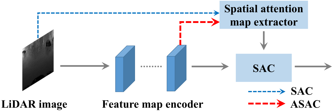
Motivation. SqueezeSegV2 (Wu et al. 2019) aligns the features between the simulation and real domains during training by Geodesic correlation alignment (Morerio, Cavazza, and Murino 2018), and employs progressive domain calibration (PDC) (Li et al. 2018b) to progressively calibrate the statistic shift during post-processing. There are some limitations of this feature alignment method: (1) The PDC module requires the DA pipeline to be designed as multi-stage. Further, it depends heavily on a good sampling of the real-world distribution to obtain accurate statistics, which is very difficult in real applications. (2) The correlation alignment only matches the second-order (covariance) statistics of different distributions, which cannot completely characterize the complex non-Gaussian deep features (Chen et al. 2020). (3) It neglects the spatial feature gap. Xu et al. 2020 (Xu et al. 2020) found that the feature distribution of LiDAR images changes drastically at different spatial locations while natural images hold a relatively identical distribution among various locations. Spatially-adaptive convolution (SAC) is proposed by learning a location-wise attention map (Xu et al. 2020). However, directly transplanting the SAC module into SRDA tasks does not guarantee better performance, because there also exists a spatial feature gap between synthetic LiDAR and real LiDAR, as shown in Figure 4.

Figure 4: Pixel-wise feature distribution at four sampled locations on the

x

coordinate channel of 5,000 projected LiDAR images from GTA-LiDAR (Wu et al. 2019) and KITTI (Geiger, Lenz, and Urtasun 2012; Wu et al. 2018a). The ordinate represents the number of images, while the abscissa represents the detailed

x

values.

In this paper, we propose statistic-invariant and spatially-adaptive feature alignment to address the above issues by (1) extracting statistics-invariant features by instance normalization (Ulyanov, Vedaldi, and Lempitsky 2016), (2) aligning the feature maps in high-dimensional space by higher-order moment matching (Chen et al. 2020), and (3) generating domain-invariant spatial attention map by improving the SAC module (Xu et al. 2020).

Statistics-Invariant Feature Extraction. To eliminate the influence of statistics variations among different instances across domains, we employ instance normalization (IN) (Ulyanov, Vedaldi, and Lempitsky 2016) to normalize each channel of the CNN feature maps, which has been demonstrated to be effective for fast style transfer in RGB images (Wu et al. 2018b). Specifically, suppose the feature maps for synthetic image $\mathbf{x}_{s}^{i}$ and real image $\mathbf{x}_{r}^{j}$ after the same activation layer are $f_{s}^{i}$ and $f_{r}^{f}$ respectively, of the same size $\mathbb{R}^{\hat{C}\times\hat{H}\times\hat{W}}$ . We can then easily conduct IN by:

		$\displaystyle\hat{f}_{s}^{i}=\frac{f_{s}^{i}-\mu(f_{s}^{i})}{\sigma(f_{s}^{i})},\hat{f}_{r}^{j}=\frac{f_{r}^{j}-\mu(f_{r}^{j})}{\sigma(f_{r}^{j})},$		(6)
		$\displaystyle\mu_{c}(f)=\frac{1}{\hat{H}\hat{W}}\sum\limits^{\hat{H}}_{h=1}\sum\limits^{\hat{W}}_{w=1}f_{chw},$
		$\displaystyle\sigma_{c}(f)=\sqrt{\frac{1}{\hat{H}\hat{W}}\sum\limits^{\hat{H}}_{h=1}\sum\limits^{\hat{W}}_{w=1}(f_{chw}-\mu_{c}(f))^{2}},$

where $\mu_{c}(f)$ and $\sigma_{c}(f)$ are the mean and variance across spatial dimensions for the $c$ -th channel.

Higher-Order Moment Matching. We employ higher-order moment matching (HOMM) (Chen et al. 2020), a discrepancy-based feature-level alignment method, to align the high-order statistics between the simulation and real domains with the following discrepancy loss:

		$\displaystyle\mathcal{L}_{HoMM}(\phi,R,\mathbf{X}_{s},\mathbf{X}_{r})=\frac{1}{N^{p}}$		(7)
		$\displaystyle\parallel\mathbb{E}_{\mathbf{x}_{s}\sim\mathbf{X}_{s}}(\phi(R(\mathbf{x}_{s})\odot\mathbf{x}_{s})^{\otimes p})-\mathbb{E}_{\mathbf{x}_{r}\sim\mathbf{X}_{r}}(\phi(\mathbf{x}_{r})^{\otimes p})\parallel^{2}_{F},$		(7)

where $\parallel\cdot\parallel_{F}$ is the Frobenius norm, $\phi(\cdot)$ and $N$ denote the activation outputs and the number of hidden neurons of the adapted layer respectively, and $\phi^{\otimes p}$ represents the $p$ -level tensor power of the vector $\phi$ .

Domain-Invariant Spatial Attention Generation. SAC (Xu et al. 2020) introduces one convolution to learn a location-wise attention map. To eliminate the spatial feature gap, we modify the structure by extracting the attention map from the previous feature maps instead of from the original images (Xu et al. 2020), as shown in Figure 5. The basic motivation is that by extracting the spatial attention map according to preceding feature maps, we can align those feature maps between different domains so that the inputs of the aligned SAC (ASAC) module are those domain-invariant features. Once the ASAC module can only see domain-invariant features during the training stage, it is more robust to generate attention map when dealing with the target data. It is worth noting that we do not need any extra operation because those feature maps have already been aligned by the employed HoMM method.

Transferable Segmentation Learning

After generating adapted LiDAR images that have similar styles to real images and aligning the features of the adapted images and real images, we can train a transferable task segmentation model $F$ based on adapted images $\{R(\mathbf{x}_{s})\odot\mathbf{x}_{s}\}$ and corresponding synthetic labels $\mathbf{Y}_{s}$ with the following focal loss (Lin et al. 2017; Wu et al. 2019):

	$\displaystyle\mathcal{L}_{seg}(F,R,\mathbf{X}_{s},\mathbf{Y}_{s})=$	$\displaystyle-\mathbb{E}_{(\mathbf{x}_{s},\mathbf{y}_{s})\sim(\mathbf{X}_{s},\mathbf{Y}_{s})}\sum\limits_{l=1}^{L}\sum\limits_{h=1}^{H}\sum\limits_{w=1}^{W}$		(8)
		$\displaystyle\mathds{1}_{[l=\mathbf{y}_{s(h,w)}]}(1-p_{l,h,w})^{\gamma}\log p_{l,h,w},$		(8)

where $p_{l,h,w}=\sigma(F_{l,h,w}(R(\mathbf{x}_{s})\odot\mathbf{x}_{s}))$ , $F_{l,h,w}(\cdot)$ is the value of $F(\cdot)$ at index $(l,h,w)$ , and $\gamma$ is a focusing parameter to adjust the rate at which well-classified examples are down-weighted. When $\gamma=0$ , focal loss equals cross-entropy loss. The advantage of focal loss is that it can deal with the imbalanced distribution of point cloud categories, e.g. more background points than foreground objects.

ePointDA Learning

The proposed ePointDA learning framework utilizes adaptation techniques to bridge the domain shift at both pixel-level and feature-level. Combining these alignment modules with transferable segmentation learning, we can obtain the overall objective loss function of ePointDA as:

		$\displaystyle\mathcal{L}_{ePointDA}(G_{s},D_{s},G_{r},D_{r},R,F)=$		(9)
		$\displaystyle\mathcal{L}_{GAN}^{r\rightarrow s}(G_{s},D_{s},\mathbf{X}_{r},\mathbf{X}_{s})+\mathcal{L}_{GAN}^{s\rightarrow r}(G_{r},D_{r},\mathbf{X}_{s},\mathbf{X}_{r})+$
		$\displaystyle\mathcal{L}_{cyc}(G_{s},G_{r},\mathbf{X}_{r},\mathbf{X}_{s})+\mathcal{L}_{mask}(R,G_{s},\mathbf{X}_{r},\mathbf{M})+$
		$\displaystyle\mathcal{L}_{HoMM}(F_{\phi},R,\mathbf{X}_{s},\mathbf{X}_{r})+\mathcal{L}_{seg}(F,R,\mathbf{X}_{s},\mathbf{Y}_{s}),$

where $F_{\phi}$ is the activation outputs of $F$ used for HoMM. The training process corresponds to solving for the target segmentation model $F$ according to:

	$\displaystyle F^{*}=$	$\displaystyle\arg\min_{F}\min_{R}\min_{D_{s},D_{r}}\max_{G_{s},G_{r}}$		(10)
		$\displaystyle\mathcal{L}_{ePointDA}(G_{s},D_{s},G_{r},D_{r},R,F).$		(10)

As shown in Eq. (9), there are 6 different losses in the overall objective loss function. The SDNR module involves 4 losses: GAN losses in two directions, cycle-consistency loss, and dropout noise rendering (DNR) loss. The feature alignment and segmentation learning modules correspond to HoMM loss and segmentation supervision loss, respectively. The GAN losses and cycle-consistency loss are used to update the CycleGAN network while the DNR loss is used to update the dropout noise prediction network. The gradient backpropagation of DNR loss would be truncated at the position of dropout noise prediction network’s inputs. Similarly, the HoMM loss and segmentation supervision loss are used to update the segmentation network, indicating that the gradient will be backpropagated only to the segmentation network.

Method	Car			Pedestrian
Method	Pre	Rec	IoU	Pre	Rec	IoU
Source-only	34.4	67.6	29.6	11.3	8.9	5.2
DAN (Long et al. 2015)	56.3	76.4	47.8	20.8	68.9	19.0
CORAL (Sun and Saenko 2016)	56.5	82.1	50.2	26.0	50.3	20.7
HoMM (Chen et al. 2020)	59.4	85.2	53.9	26.2	66.8	23.2
ADDA (Tzeng et al. 2017)	56.7	83.5	50.7	24.7	58.5	21.0
CyCADA (Hoffman et al. 2018)	40.9	72.1	35.3	17.8	52.4	15.3
SqueezeSegV2 (Wu et al. 2019)	-	-	57.4	-	-	23.5
ePointDA (Ours)	75.2	84.7	66.2	28.7	65.2	24.8
Oracle (SqueezeSegV2)	76.7	92.1	71.9	28.5	82.3	26.9
Oracle+SAC	78.4	91.4	73.1	28.9	84.5	27.4
Oracle+SAC+HHead	77.8	93.1	73.5	29.3	86.6	28.0

Table 1: Comparison with the state-of-the-art DA methods for LiDAR point cloud segmentation from GTA-LiDAR to KITTI, where +ASAC denotes using the spatial feature aligned SAC module, and +HHead denotes replacing the CRF layer with an conv layer. The best IoU of each category trained on the simulation domain is emphasized in bold.

Experiments

In this section, we introduce the experimental settings and compare ePointDA with state-of-the-art approaches, followed by series of ablation studies and visualizations.

Experimental Settings

Datasets. We perform SRDA from synthetic GTA-LiDAR (Wu et al. 2019) to real KITTI (Geiger, Lenz, and Urtasun 2012) and SemanticKITTI (Behley et al. 2019) datasets for LiDAR point cloud segmentation. GTA-LiDAR (Wu et al. 2019) contains 100,000 LiDAR point clouds synthesized in GTA-V. The depth segmentation map is generated by (Krähenbühl 2018) and the Image-LiDAR registration is conducted by (Yue et al. 2018). There are one label and $x,y,z$ coordinates for each point in the synthetic point cloud, without dropout noise and intensity.

KITTI (Geiger, Lenz, and Urtasun 2012; Wu et al. 2018a) contains 10,848 samples with point-wise labels obtained from the original 3D bounding boxes. As in SqueezeSegV2 (Wu et al. 2019), we split the dataset into a training set with 8,057 samples and a test set with 2,791 samples.

SemanticKITTI (Behley et al. 2019) is a recently released large-scale dataset for LiDAR point-cloud segmentation with 21 sequences and 43,442 densely annotated scans. Following (Behley et al. 2019), we employ sequences-{0-7} and {9, 10} (19,130 scans) for training, sequence-08 (4,071 scans) for validation, and sequences-{11-21} (20,351 scans) for testing.

Since there are only two categories in the GTA-LiDAR dataset, i.e. car and pedestrian, we select the images in KITTI and SemanticKITTI that contain these two categories⁶⁶ 6 For SemanticKITTI, we combine the original {car, truck, bus} and {person} respectively as the car and pedestrian categories. and report the segmentation adaptation results. Constructing a synthetic dataset with more categories for LiDAR point cloud segmentation and performing SRDA remains our future work.

Method	Car			Pedestrian
Method	Pre	Rec	IoU	Pre	Rec	IoU
Source-only	63.8	40.8	33.2	3.9	43.7	3.7
DAN (Long et al. 2015)	73.6	66.4	53.6	12.1	28.0	9.2
CORAL (Sun and Saenko 2016)	73.4	71.3	56.6	8.9	30.0	7.4
HoMM (Chen et al. 2020)	73.8	69.5	55.7	11.7	23.8	8.5
ADDA (Tzeng et al. 2017)	65.3	84.5	58.3	13.7	30.1	10.4
CyCADA (Hoffman et al. 2018)	78.3	48.1	42.4	9.7	34.8	8.2
SqueezeSegV2 (Wu et al. 2019)	65.9	93.8	63.2	14.9	46.9	12.8
ePointDA (Ours)	77.9	88.5	70.7	14.7	51.2	12.9
Oracle (SqueezeSegV2)	93.9	96.4	90.7	41.4	50.0	29.3
Oracle+SAC	92.9	98.2	91.4	47.0	46.4	30.4
Oracle+SAC+HHead	93.4	98.5	92.1	49.3	48.8	32.5

Table 2: Comparison with the state-of-the-art DA methods from GTA-LiDAR to SemanticKITTI.

Evaluation Metrics. Similar to (Wu et al. 2018a), we employ precision, recall, and intersection-over-union (IoU) to evaluate the class-level segmentation results by comparing the predicted results with ground-truth labels point-wisely: $Pre_{l}=\frac{|\mathcal{P}_{l}\cap\mathcal{G}_{l}|}{|\mathcal{P}_{l}},Rec_{l}=\frac{|\mathcal{P}_{l}\cap\mathcal{G}_{l}|}{|\mathcal{G}_{l}},IoU_{l}=\frac{|\mathcal{P}_{l}\cap\mathcal{G}_{l}|}{|\mathcal{P}_{l}\cup\mathcal{G}_{l}|},$ where $\mathcal{P}_{l}$ and $\mathcal{G}_{l}$ respectively denote the predicted and ground-truth point sets that belong to class- $l$ , and $|\cdot|$ represents the cardinality of a set. Larger precision, recall, and IoU values represent better results. We employ IoU as the primary metric.

Baselines. To the best of our knowledge, ePointDA is the first end-to-end framework for simulation-to-real LiDAR point cloud segmentation. To demonstrate its effectiveness, we compare to baselines of three types: (1) source-only, directly transferring the model trained on the simulation domain; (2) SqueezeSegV2 (Wu et al. 2019), one state-of-the-art SRDA method for LiDAR point cloud segmentation; (3) state-of-the-art DA methods for RGB image classification and segmentation tasks: DAN (Long et al. 2015), CORAL (Sun and Saenko 2016), ADDA (Tzeng et al. 2017), CyCADA (Hoffman et al. 2018), and HoMM (Chen et al. 2020). For comparison, we also report the oracle result, i.e. the segmentation model is trained also on the real domain, which can be viewed as an upper bound.

Implementation Details. For SDNR, we employ the same architecture as SqueezeSegV2 (Wu et al. 2019) except the final layer which is changed to be a binary mask classification. The segmentation network is shown in Figure 3, which replaces all the standard convolution and batch normalization in SqueezeSegV2 (Wu et al. 2019) with spatially-adaptive convolution and instance normalization. Our model is implemented using TensorFlow with the same hyper-parameters as (Wu et al. 2019). We use stochastic gradient descent (SGD) as the optimizer with a momentum of 0.9 and a batch size of 20. The initial learning rate is 0.05 with a decay factor of 0.5 for every 20,000 steps. As in (Lin et al. 2017; Wu et al. 2019), the focusing parameter $\gamma$ in Eq. (8) is set to $2$ . Besides, in practical implementation, the complexity of calculating the higher-order tensor $\phi^{\otimes p}$ in Eq. (7) would explode (i.e. $\mathcal{O}(L^{p})$ ) as order $p$ increases. Following (Chen et al. 2020), we use the Monte Carlo estimation as an approximation.

Method	Car			Pedestrian
Method	Pre	Rec	IoU	Pre	Rec	IoU
Baseline	59.6	83.2	53.1	21.5	77.1	20.2
+SDNR	65.7	84.8	58.7	24.7	75.4	22.8
+SDNR+IN	69.3	86.9	62.7	28.8	57.6	23.8
+SDNR+IN+HoMM	73.4	81.9	63.4	29.4	56.0	23.9
+SDNR+IN+HoMM+ASAC	72.1	85.6	64.2	31.2	57.5	25.3
+SDNR+IN+HoMM+ASAC+HHead	75.2	84.7	66.2	28.7	65.2	24.8

Table 3: Ablation study on different modules, where Baseline denotes a simplified SqueezeSegV2 model (Wu et al. 2019) for fair comparison taking the Cartesian coordinates as input and using batch normalization, frequency-based DNR, and Geodesic correlation alignment.

Comparison with the State-of-the-art

The performance comparisons between ePointDA and the state-of-the-art DA methods are shown in Table 1 and Table 2. From the results, we can observe that⁷⁷ 7 Since pedestrian is synthesized by a very simple physical model in the GTA-LiDAR dataset (Wu et al. 2019), which often represents pedestrians as cylinders, we mainly focus on the IoU of the “car” class for evaluation and comparison.:

(1) Because of the presence of domain shift, the joint probability distributions of observed LiDAR point clouds and corresponding labels significantly vary between the simulation and real domains. As a result, the source-only method that does not consider the domain gap obtains the worst IoU performance, which motivates the research on domain adaptation.

(2) On one hand, when directly applied to the LiDAR SRDA task, the traditional RGB-image-targeted DA methods outperform the source-only setting. Among these methods, discrepancy-based methods (DAN, CORAL, HoMM) and adversarial discriminative methods (ADDA) obtain much better results than adversarial generative methods (CyCADA). Besides feature-level alignment, CyCADA also conducts pixel-level alignment by CycleGAN (Zhu et al. 2017), which is mainly designed to translate natural images’ colors and textures among different domains. Since the projected 2D LiDAR images are mainly about geometric information, which is quite different from RGB images, the translated LiDAR images by CycleGAN are of low quality. On the other hand, these RGB-image-targeted DA methods do not outperform SqueezeSegV2 (Wu et al. 2019), one SRDA method specially designed for LiDAR point cloud segmentation. This is reasonable, because they do not consider the specific characteristics of LiDAR point clouds, such as dropout noise, the intensity of synthetic data, and the statistics difference between simulation and real domains.

(3) ePointDA performs the best among all adaptation settings. For example, the performance improvements of ePointDA over SqueezeSegV2 are 8.8% and 7.5% on KITTI and SemanticKITTI, respectively. These results demonstrate the superiority of ePointDA relative to state-of-the-art DA approaches for LiDAR point cloud segmentation⁸⁸ 8 One may argue that ePointDA contains some extra modules (i.e. Aligned SAC and one more conv layer), which might be unfair to compare with SqueeseSegV2. Even if we drop these modules, i.e. +SDNR+IN+HoMM in Table 3, our method still outperforms SqueeseSegV2 by a large margin (63.4 vs. 57.4).. The performance improvements benefit from the advantages of ePointDA: pixel-level alignment by self-supervised dropout noise rendering and feature-level alignment by higher-order moment matching with statistics-invariant features and domain-invariant spatial attentions.

(4) There is still a large performance gap between ePointDA and the oracle method. As demonstrated in (Xu et al. 2020), the SAC module can improve the oracle performance. Replacing the CRF layer in SqueezeSegV2 with a conv layer also works under the oracle setting.

DNR	Norm	Car			Pedestrian
DNR	Norm	Pre	Rec	IoU	Pre	Rec	IoU
Frequency (Wu et al. 2019)	BN	59.6	83.2	53.1	21.5	77.1	20.2
	IN	63.5	83.6	56.5	25.4	65.6	22.4
	LN	60.2	84.6	54.3	24.3	65.5	21.5
	GN	61.4	83.5	54.7	26.0	50.3	20.7
Learned (ours)	BN	65.7	84.8	58.7	24.7	75.4	22.8
	IN	69.3	86.9	62.7	28.8	57.6	23.8
	LN	65.1	88.6	60.1	27.3	59.3	22.9
	GN	64.1	88.9	59.3	27.8	61.4	23.7

Table 4: Ablation study on different normalization schemes using both frequency-based DNR and our learned DNR without feature alignment. ‘BN’, ‘IN’, ‘LN’, ‘GN’ are short for batch normalization, instance normalization, layer normalization, and group normalization, respectively.

Ablation Study

We conduct a series of ablation studies when adapting from GTA-LiDAR to KITTI. First, we incrementally investigate the effectiveness of different modules in ePointDA. From the results in Table 3, we can observe that: (1) adding each module can improve the IoU scores, which demonstrates that all the modules contained in ePointDA contribute to the SRDA task; (2) among all these modules, SDNR provides the highest performance improvement (5.6%), which demonstrates the important role that dropout noise plays in the domain gap between the simulation and real domains and the necessity of exploring effective DNR model.

Second, we explore the differences caused by various normalization schemes, including batch normalization (BN) (Ioffe and Szegedy 2015), instance normalization (IN) (Ulyanov, Vedaldi, and Lempitsky 2016), layer normalization (LN) (Ba, Kiros, and Hinton 2016), and group normalization (GN) (Wu and He 2018). From Table 4, it is clear that IN, LN, and GN all outperform BN. The relative poor performance of BN results from the statistics gap between the simulation and real domains. IN, LN, and GN can all eliminate such gap to some extent (Wu et al. 2018b) and thus achieve better DA results than BN.

Method	Car			Pedestrian
Method	Pre	Rec	IoU	Pre	Rec	IoU
Baseline	73.4	81.9	63.4	29.4	56.0	23.9
SAC (Xu et al. 2020)	68.5	83.2	60.2	25.2	62.4	21.9
ASAC (ours)	72.1	85.6	64.2	31.2	57.5	25.3

Table 5: Comparison between ordinary SAC (Xu et al. 2020) and our aligned SAC (ASAC). Baseline corresponds the “+SDNR+IN+HoMM” setting in Table 3.

Third, we compare our aligned SAC (ASAC) and the ordinary SAC (Xu et al. 2020) in Table 5. Without considering the spatial feature gap, simply incorporating the ordinary SAC can result in a significant performance drop. Our aligned modification helps address this issue and thus improves the DA performance.

Finally, we study the influence of convolution (conv) layers appended to the last deconvolution layer of the segmentation network. From Table 6, we can conclude that adding 2 conv layers performs the best. As stated in (Li et al. 2019; Yu and Koltun 2016; Dai et al. 2017; Dai et al. 2016), the receptive field can affect the network’s effectiveness. As the number of conv layers increases, the segmentation results become better; after reaching the best receptive field (2 conv layers), the segmentation results decrease gradually.

#Conv	Car			Pedestrian
#Conv	Pre	Rec	IoU	Pre	Rec	IoU
1	72.1	85.6	64.2	31.2	57.5	25.3
2	75.2	84.7	66.2	28.7	65.2	24.8
3	74.1	82.3	63.8	26.9	64.8	23.4
4	70.6	83.4	61.9	25.1	59.7	21.5
5	68.6	84.0	60.7	26.5	52.3	21.3

Table 6: Ablation study on the number of convolution layers (#Conv) that are appended to the last deconvolution layer. This experiment is conducted after dropout noise rendering and feature alignment, i.e. +SDNR+IN+HoMM+ASAC.

Visualization

First, we qualitatively visualize the LiDAR point cloud segmentation results from GTA-LiDAR to KITTI in Figure 6. We can clearly see that after adaptation by ePointDA, the segmentation results are improved notably as compared to source-only and SqueezeSegV2 (Wu et al. 2019). For example, in the first column, ePointDA avoids falsely detecting some pedestrians. In the second column, ePointDA classifies the cyclist as a pedestrian, which is reasonable because there is no cyclist in the GTA-LiDAR dataset. Please note that there does exist some missing objects in the original annotations, such as the car on the right corner in the third column. This is either because some objects are not labeled in the original 3D point clouds, or because some information is missing during the projection from 3D point clouds to 2D images. For fair comparison, we used the same setting as SqueezeSegV2. We will refine the annotations in our future work to make the proposed method more practical.

Second, we visualize the DNR results on KITTI. From the results in Figure 7, it is clear that the rendered dropout noise is very close to the ground truth, which demonstrates the effectiveness of our SDNR method.

Conclusion

In this paper, we proposed an end-to-end simulation-to-real domain adaptation (SRDA) framework, named ePointDA, for LiDAR point cloud segmentation. By explicitly rendering dropout noise for the real domain in a self-supervised manner and spatially aligning higher-level moments between the simulation and real domains, ePointDA bridges the domain shift at both the pixel-level and feature-level. Further, ePointDA does not require prior statistics of the real domain, which makes it more robust and practical. The extensive experiments adapting from synthetic GTA-LiDAR to real KITTI and SemanticKITTI demonstrated that ePointDA significantly outperforms the state-of-the-art SRDA methods. The proposed ePointDA can be easily applied to other applications, such as robotics grasping. It can also be applied to other depth data, like the depth from Kinect, which has similar properties to LiDAR. Another promising extension is the specific adaptation setting where the source and target domains have different channels, such as adapting from RGB to RGB-Depth.

In future studies, we plan to construct a large-scale synthetic dataset for LiDAR point cloud segmentation containing more compatible categories with SemanticKITTI and extend our framework to corresponding SRDA tasks. We will explore multi-modal domain adaptation by jointly modeling multiple modalities, such as image and LiDAR.

Acknowledgments

This work is supported by the National Natural Science Foundation of China (No. 61701273), Berkeley DeepDrive, and the Zhongguancun Haihua Institute for Frontier Information Technology.

References

Achituve, Maron, and Chechik (2021) Achituve, I.; Maron, H.; and Chechik, G. 2021. Self-Supervised Learning for Domain Adaptation on Point Clouds. In WACV, 123–133.
Ba, Kiros, and Hinton (2016) Ba, J. L.; Kiros, J. R.; and Hinton, G. E. 2016. Layer normalization. arXiv:1607.06450v1 [stat.ML].
Behley et al. (2019) Behley, J.; Garbade, M.; Milioto, A.; Quenzel, J.; Behnke, S.; Stachniss, C.; and Gall, J. 2019. SemanticKITTI: A dataset for semantic scene understanding of lidar sequences. In ICCV, 9297–9307.
Caltagirone et al. (2017) Caltagirone, L.; Scheidegger, S.; Svensson, L.; and Wahde, M. 2017. Fast LIDAR-based road detection using fully convolutional neural networks. In IV, 1019–1024.
Carlucci et al. (2019) Carlucci, F. M.; D’Innocente, A.; Bucci, S.; Caputo, B.; and Tommasi, T. 2019. Domain generalization by solving jigsaw puzzles. In CVPR, 2229–2238.
Chen et al. (2020) Chen, C.; Fu, Z.; Chen, Z.; Jin, S.; Cheng, Z.; Jin, X.; and Hua, X.-S. 2020. HoMM: Higher-order Moment Matching for Unsupervised Domain Adaptation. In AAAI, 3422–3429.
Dai et al. (2016) Dai, J.; Li, Y.; He, K.; and Sun, J. 2016. R-fcn: Object detection via region-based fully convolutional networks. In NeurIPS, 379–387.
Dai et al. (2017) Dai, J.; Qi, H.; Xiong, Y.; Li, Y.; Zhang, G.; Hu, H.; and Wei, Y. 2017. Deformable convolutional networks. In ICCV, 764–773.
Dosovitskiy et al. (2017) Dosovitskiy, A.; Ros, G.; Codevilla, F.; Lopez, A.; and Koltun, V. 2017. CARLA: An open urban driving simulator. In CoRL, 1–16.
Dovrat, Lang, and Avidan (2019) Dovrat, O.; Lang, I.; and Avidan, S. 2019. Learning to sample. In CVPR, 2760–2769.
Feng, Xu, and Tao (2019) Feng, Z.; Xu, C.; and Tao, D. 2019. Self-Supervised Representation Learning From Multi-Domain Data. In ICCV, 3245–3255.
Geiger, Lenz, and Urtasun (2012) Geiger, A.; Lenz, P.; and Urtasun, R. 2012. Are we ready for autonomous driving? the kitti vision benchmark suite. In CVPR, 3354–3361.
Goodfellow et al. (2014) Goodfellow, I.; Pouget-Abadie, J.; Mirza, M.; Xu, B.; Warde-Farley, D.; Ozair, S.; Courville, A.; and Bengio, Y. 2014. Generative adversarial nets. In NeurIPS, 2672–2680.
Hoffman et al. (2018) Hoffman, J.; Tzeng, E.; Park, T.; Zhu, J.-Y.; Isola, P.; Saenko, K.; Efros, A. A.; and Darrell, T. 2018. CyCADA: Cycle-Consistent Adversarial Domain Adaptation. In ICML, 1994–2003.
Huang, Wang, and Neumann (2018) Huang, Q.; Wang, W.; and Neumann, U. 2018. Recurrent slice networks for 3d segmentation of point clouds. In CVPR, 2626–2635.
Ioffe and Szegedy (2015) Ioffe, S.; and Szegedy, C. 2015. Batch Normalization: Accelerating Deep Network Training by Reducing Internal Covariate Shift. In ICML, 448–456.
Jiang et al. (2019) Jiang, L.; Zhao, H.; Liu, S.; Shen, X.; Fu, C.-W.; and Jia, J. 2019. Hierarchical point-edge interaction network for point cloud semantic segmentation. In ICCV, 10433–10441.
Jiang and Saripalli (2020) Jiang, P.; and Saripalli, S. 2020. LiDARNet: A Boundary-Aware Domain Adaptation Model for Lidar Point Cloud Semantic Segmentation. arXiv:2003.01174v2 [cs.CV].
Klokov and Lempitsky (2017) Klokov, R.; and Lempitsky, V. 2017. Escape from cells: Deep kd-networks for the recognition of 3d point cloud models. In ICCV, 863–872.
Krähenbühl (2018) Krähenbühl, P. 2018. Free supervision from video games. In CVPR, 2955–2964.
Landrieu and Simonovsky (2018) Landrieu, L.; and Simonovsky, M. 2018. Large-scale point cloud semantic segmentation with superpoint graphs. In CVPR, 4558–4567.
Le and Duan (2018) Le, T.; and Duan, Y. 2018. Pointgrid: A deep network for 3d shape understanding. In CVPR, 9204–9214.
Lee et al. (2019) Lee, S.; Kim, D.; Kim, N.; and Jeong, S.-G. 2019. Drop to adapt: Learning discriminative features for unsupervised domain adaptation. In ICCV, 91–100.
Lei, Akhtar, and Mian (2019) Lei, H.; Akhtar, N.; and Mian, A. 2019. Octree guided CNN with spherical kernels for 3D point clouds. In CVPR, 9631–9640.
Li, Chen, and Hee Lee (2018) Li, J.; Chen, B. M.; and Hee Lee, G. 2018. So-net: Self-organizing network for point cloud analysis. In CVPR, 9397–9406.
Li et al. (2018a) Li, Y.; Bu, R.; Sun, M.; Wu, W.; Di, X.; and Chen, B. 2018a. Pointcnn: Convolution on x-transformed points. In NeurIPS, 820–830.
Li et al. (2019) Li, Y.; Chen, Y.; Wang, N.; and Zhang, Z. 2019. Scale-aware trident networks for object detection. In ICCV, 6054–6063.
Li et al. (2018b) Li, Y.; Wang, N.; Shi, J.; Hou, X.; and Liu, J. 2018b. Adaptive Batch Normalization for practical domain adaptation. PR 80: 109–117.
Lin et al. (2020) Lin, C.; Zhao, S.; Meng, L.; and Chua, T.-S. 2020. Multi-Source Domain Adaptation for Visual Sentiment Classification. In AAAI, 2661–2668.
Lin et al. (2017) Lin, T.-Y.; Goyal, P.; Girshick, R.; He, K.; and Dollár, P. 2017. Focal loss for dense object detection. In ICCV, 2980–2988.
Liu et al. (2019a) Liu, Y.; Fan, B.; Meng, G.; Lu, J.; Xiang, S.; and Pan, C. 2019a. DensePoint: Learning densely contextual representation for efficient point cloud processing. In ICCV, 5239–5248.
Liu et al. (2019b) Liu, Z.; Tang, H.; Lin, Y.; and Han, S. 2019b. Point-Voxel CNN for efficient 3D deep learning. In NeurIPS, 963–973.
Long et al. (2015) Long, M.; Cao, Y.; Wang, J.; and Jordan, M. 2015. Learning transferable features with deep adaptation networks. In ICML, 97–105.
Lyu, Huang, and Zhang (2020) Lyu, Y.; Huang, X.; and Zhang, Z. 2020. Learning to Segment 3D Point Clouds in 2D Image Space. In CVPR, 12252–12261.
Mao, Wang, and Li (2019) Mao, J.; Wang, X.; and Li, H. 2019. Interpolated convolutional networks for 3d point cloud understanding. In ICCV, 1578–1587.
Meng et al. (2019) Meng, H.-Y.; Gao, L.; Lai, Y.-K.; and Manocha, D. 2019. VV-Net: Voxel vae net with group convolutions for point cloud segmentation. In ICCV, 8500–8508.
Milioto et al. (2019) Milioto, A.; Vizzo, I.; Behley, J.; and Stachniss, C. 2019. Rangenet++: Fast and accurate lidar semantic segmentation. In IROS, 4213–4220.
Morerio, Cavazza, and Murino (2018) Morerio, P.; Cavazza, J.; and Murino, V. 2018. Minimal-Entropy Correlation Alignment for Unsupervised Deep Domain Adaptation. In ICLR, 1–15.
Patel et al. (2015) Patel, V. M.; Gopalan, R.; Li, R.; and Chellappa, R. 2015. Visual domain adaptation: A survey of recent advances. IEEE SPM 32(3): 53–69.
Peng et al. (2019) Peng, X.; Bai, Q.; Xia, X.; Huang, Z.; Saenko, K.; and Wang, B. 2019. Moment matching for multi-source domain adaptation. In ICCV, 1406–1415.
Qi et al. (2017a) Qi, C. R.; Su, H.; Mo, K.; and Guibas, L. J. 2017a. Pointnet: Deep learning on point sets for 3d classification and segmentation. In CVPR, 652–660.
Qi et al. (2017b) Qi, C. R.; Yi, L.; Su, H.; and Guibas, L. J. 2017b. Pointnet++: Deep hierarchical feature learning on point sets in a metric space. In NeurIPS, 5099–5108.
Qin et al. (2019) Qin, C.; You, H.; Wang, L.; Kuo, C.-C. J.; and Fu, Y. 2019. PointDAN: A multi-scale 3D domain adaption network for point cloud representation. In NeurIPS, 7190–7201.
Richter et al. (2016) Richter, S. R.; Vineet, V.; Roth, S.; and Koltun, V. 2016. Playing for data: Ground truth from computer games. In ECCV, 102–118.
Rist, Enzweiler, and Gavrila (2019) Rist, C. B.; Enzweiler, M.; and Gavrila, D. M. 2019. Cross-Sensor Deep Domain Adaptation for LiDAR Detection and Segmentation. In IV, 1535–1542.
Russo et al. (2018) Russo, P.; Carlucci, F. M.; Tommasi, T.; and Caputo, B. 2018. From source to target and back: symmetric bi-directional adaptive gan. In CVPR, 8099–8108.
Saleh et al. (2019) Saleh, K.; Abobakr, A.; Attia, M.; Iskander, J.; Nahavandi, D.; Hossny, M.; and Nahvandi, S. 2019. Domain Adaptation for Vehicle Detection from Bird’s Eye View LiDAR Point Cloud Data. In ICCVW, 1–8.
Sankaranarayanan et al. (2018) Sankaranarayanan, S.; Balaji, Y.; Castillo, C. D.; and Chellappa, R. 2018. Generate to adapt: Aligning domains using generative adversarial networks. In CVPR, 8503–8512.
Shrivastava et al. (2017) Shrivastava, A.; Pfister, T.; Tuzel, O.; Susskind, J.; Wang, W.; and Webb, R. 2017. Learning from simulated and unsupervised images through adversarial training. In CVPR, 2107–2116.
Sun, Feng, and Saenko (2016) Sun, B.; Feng, J.; and Saenko, K. 2016. Return of frustratingly easy domain adaptation. In AAAI, 2058–2065.
Sun and Saenko (2016) Sun, B.; and Saenko, K. 2016. Deep CORAL: Correlation Alignment for Deep Domain Adaptation. In ECCVW, 443–450.
Sun et al. (2019) Sun, Y.; Tzeng, E.; Darrell, T.; and Efros, A. A. 2019. Unsupervised Domain Adaptation through Self-Supervision. arXiv:1909.11825v2 [cs.LG].
Te et al. (2018) Te, G.; Hu, W.; Zheng, A.; and Guo, Z. 2018. Rgcnn: Regularized graph cnn for point cloud segmentation. In ACM MM, 746–754.
Tripathi et al. (2019) Tripathi, S.; Chandra, S.; Agrawal, A.; Tyagi, A.; Rehg, J. M.; and Chari, V. 2019. Learning to generate synthetic data via compositing. In CVPR, 461–470.
Tzeng et al. (2017) Tzeng, E.; Hoffman, J.; Saenko, K.; and Darrell, T. 2017. Adversarial discriminative domain adaptation. In CVPR, 2962–2971.
Ulyanov, Vedaldi, and Lempitsky (2016) Ulyanov, D.; Vedaldi, A.; and Lempitsky, V. 2016. Instance normalization: The missing ingredient for fast stylization. arXiv:1607.08022v3 [cs.CV].
Wang et al. (2019a) Wang, B.; Wu, V.; Wu, B.; and Keutzer, K. 2019a. LATTE: accelerating lidar point cloud annotation via sensor fusion, one-click annotation, and tracking. In ITSC, 265–272.
Wang et al. (2019b) Wang, L.; Huang, Y.; Hou, Y.; Zhang, S.; and Shan, J. 2019b. Graph attention convolution for point cloud semantic segmentation. In CVPR, 10296–10305.
Wang et al. (2017) Wang, P.-S.; Liu, Y.; Guo, Y.-X.; Sun, C.-Y.; and Tong, X. 2017. O-cnn: Octree-based convolutional neural networks for 3d shape analysis. ACM TOG 36(4): 1–11.
Wang et al. (2019c) Wang, Y.; Sun, Y.; Liu, Z.; Sarma, S. E.; Bronstein, M. M.; and Solomon, J. M. 2019c. Dynamic graph cnn for learning on point clouds. ACM TOG 38(5): 1–12.
Wu et al. (2018a) Wu, B.; Wan, A.; Yue, X.; and Keutzer, K. 2018a. Squeezeseg: Convolutional neural nets with recurrent crf for real-time road-object segmentation from 3d lidar point cloud. In ICRA, 1887–1893.
Wu et al. (2019) Wu, B.; Zhou, X.; Zhao, S.; Yue, X.; and Keutzer, K. 2019. Squeezesegv2: Improved model structure and unsupervised domain adaptation for road-object segmentation from a lidar point cloud. In ICRA, 4376–4382.
Wu and He (2018) Wu, Y.; and He, K. 2018. Group normalization. In ECCV, 3–19.
Wu et al. (2018b) Wu, Z.; Han, X.; Lin, Y.-L.; Gokhan Uzunbas, M.; Goldstein, T.; Nam Lim, S.; and Davis, L. S. 2018b. Dcan: Dual channel-wise alignment networks for unsupervised scene adaptation. In ECCV, 518–534.
Xu et al. (2020) Xu, C.; Wu, B.; Wang, Z.; Zhan, W.; Vajda, P.; Keutzer, K.; and Tomizuka, M. 2020. SqueezeSegV3: Spatially-Adaptive Convolution for Efficient Point-Cloud Segmentation. In ECCV, 1–19.
Xu et al. (2018) Xu, Y.; Fan, T.; Xu, M.; Zeng, L.; and Qiao, Y. 2018. Spidercnn: Deep learning on point sets with parameterized convolutional filters. In ECCV, 87–102.
Yu and Koltun (2016) Yu, F.; and Koltun, V. 2016. Multi-scale context aggregation by dilated convolutions. In ICLR, 1–13.
Yue et al. (2018) Yue, X.; Wu, B.; Seshia, S. A.; Keutzer, K.; and Sangiovanni-Vincentelli, A. L. 2018. A lidar point cloud generator: from a virtual world to autonomous driving. In ICMR, 458–464.
Zhang, Hua, and Yeung (2019) Zhang, Z.; Hua, B.-S.; and Yeung, S.-K. 2019. Shellnet: Efficient point cloud convolutional neural networks using concentric shells statistics. In ICCV, 1607–1616.
Zhao et al. (2018a) Zhao, H.; Zhang, S.; Wu, G.; Moura, J. M.; Costeira, J. P.; and Gordon, G. J. 2018a. Adversarial multiple source domain adaptation. In NeurIPS, 8559–8570.
Zhao et al. (2019a) Zhao, S.; Li, B.; Yue, X.; Gu, Y.; Xu, P.; Hu, R.; Chai, H.; and Keutzer, K. 2019a. Multi-source Domain Adaptation for Semantic Segmentation. In NeurIPS, 7285–7298.
Zhao et al. (2019b) Zhao, S.; Lin, C.; Xu, P.; Zhao, S.; Guo, Y.; Krishna, R.; Ding, G.; and Keutzer, K. 2019b. CycleEmotionGAN: Emotional Semantic Consistency Preserved CycleGAN for Adapting Image Emotions. In AAAI, 2620–2627.
Zhao et al. (2020a) Zhao, S.; Wang, G.; Zhang, S.; Gu, Y.; Li, Y.; Song, Z.; Xu, P.; Hu, R.; Chai, H.; and Keutzer, K. 2020a. Multi-source Distilling Domain Adaptation. In AAAI, 12975–12983.
Zhao et al. (2021) Zhao, S.; Xiao, Y.; Guo, J.; Yue, X.; Yang, J.; Krishna, R.; Xu, P.; and Keutzer, K. 2021. Curriculum CycleGAN for Textual Sentiment Domain Adaptation with Multiple Sources. In WWW, to appear.
Zhao et al. (2020b) Zhao, S.; Yue, X.; Zhang, S.; Li, B.; Zhao, H.; Wu, B.; Krishna, R.; Gonzalez, J. E.; Sangiovanni-Vincentelli, A. L.; Seshia, S. A.; et al. 2020b. A Review of Single-Source Deep Unsupervised Visual Domain Adaptation. IEEE TNNLS to appear.
Zhao et al. (2018b) Zhao, S.; Zhao, X.; Ding, G.; and Keutzer, K. 2018b. EmotionGAN: unsupervised domain adaptation for learning discrete probability distributions of image emotions. In ACM MM, 1319–1327.
Zhu et al. (2017) Zhu, J.-Y.; Park, T.; Isola, P.; and Efros, A. A. 2017. Unpaired Image-To-Image Translation Using Cycle-Consistent Adversarial Networks. In ICCV, 2223–2232.
Zhuo et al. (2017) Zhuo, J.; Wang, S.; Zhang, W.; and Huang, Q. 2017. Deep Unsupervised Convolutional Domain Adaptation. In ACM MM, 261–269.