跳到论文正文
W Papers独立论文阅读器 arXiv:2009.03360 论文正文 计算阅读时间 · 0%
引用这篇论文根据当前论文元数据生成,正式投稿前建议核对。


License: arXiv.org perpetual non-exclusive license
arXiv:2009.03360v2 [math.AP] 07 Oct 2020

The Peskin Problem with Viscosity ContrastThanks: ∗partially supported by the grant MTM2017-89976-P (Spain), by the ERC through the Starting Grant project H2020-EU.1.1.-639227, and by the AMS-Simons Travel Grant.Thanks: §partially supported by the NSF grant DMS-1907583, 2042144 (USA) and the Math+X award from the Simons Foundation.Thanks: partially supported by the NSF grant DMS-1764177 (USA)

Eduardo García-Juárez†,∗ , Yoichiro Mori†,§ and Robert M. Strain†,¶ Address: †Department of Mathematics, University of Pennsylvania, David Rittenhouse Lab., 209 South 33rd St., Philadelphia, PA 19104, USA. ∗edugar@math.upenn.edu§y1mori@math.upenn.edustrain@math.upenn.edu
Abstract.

The Peskin problem models the dynamics of a closed elastic filament immersed in an incompressible fluid. In this paper, we consider the case when the inner and outer viscosities are possibly different. This viscosity contrast adds further non-local effects to the system through the implicit non-local relation between the net force and the free interface. We prove the first global well-posedness result for the Peskin problem in this setting. The result applies for medium size initial interfaces in critical spaces and shows instant analytic smoothing. We carefully calculate the medium size constraint on the initial data. These results are new even without viscosity contrast.

Key words and phrases:
Peskin problem, Fluid-Structure interface, viscosity contrast, global regularity, critical regularity, immersed boundary problem, Stokes flow, fractional Laplacian, solvability, stability.
2010 Mathematics Subject Classification
35Q35, 35C10, 35C15, 35R11, 35R35, 76D07.

1. Introduction

Fluid structure interaction (FSI) problems in which an elastic structure interacts with a surrounding fluid are found in many areas of science and engineering. Many numerical algorithms have been developed for such problems, and the scientific computing of FSI problems continues to be a very active area of research [13, 19, 29, 24]. The Peskin problem, considered in this paper, is arguably one of the simplest FSI problems, and has been used extensively in physical modeling as well as in the development of numerical algorithms as a prototypical test problem.

1.1. Formulation

Consider the following fluid problem in ℝ2\mathbb{R}^{2}. A closed elastic string Γ\Gamma encloses a simply connected bounded domain Ω1⊂ℝ2\Omega_{1}\subset\mathbb{R}^{2} filled with a Stokes fluid with viscosity μ1\mu_{1}. The outside region Ω2=ℝ2\(Ω1∪Γ)\Omega_{2}=\mathbb{R}^{2}\backslash(\Omega_{1}\cup\Gamma) is filled with a Stokes fluid of viscosity μ2\mu_{2}. The equations satisfied are:

(1.1) μ1​Δ​𝒖−∇p\displaystyle\mu_{1}\Delta\boldsymbol{u}-\nabla p =𝟎​ in ​Ω1\displaystyle=\boldsymbol{0}\text{ in }\Omega_{1}
(1.2) μ2​Δ​𝒖−∇p\displaystyle\mu_{2}\Delta\boldsymbol{u}-\nabla p =𝟎​ in ​Ω2\displaystyle=\boldsymbol{0}\text{ in }\Omega_{2}
(1.3) ∇⋅𝒖\displaystyle\nabla\cdot\boldsymbol{u} =0​ in ​ℝ2\Γ.\displaystyle=0\text{ in }\mathbb{R}^{2}\backslash\Gamma.

Here 𝒖\boldsymbol{u} is the velocity field and pp is the pressure.

We must specify the interface conditions at Γ\Gamma. Parametrize Γ\Gamma by the material or Lagrangian coordinate θ∈𝕊=ℝ/(2​π​ℤ)\theta\in\mathbb{S}=\mathbb{R}/(2\pi\mathbb{Z}), and let 𝓧⁡(θ,t)\boldsymbol{\mathcal{X}}(\theta,t) denote the coordinate position of Γ\Gamma at time tt. The parametrization is in the counter-clockwise direction, so that the interior region Ω1\Omega_{1} is on the left hand side of the tangent vector ∂𝓧/∂θ\partial\boldsymbol{\mathcal{X}}/\partial\theta. For any quantity ww defined on Ω1\Omega_{1} and Ω2\Omega_{2}, we set:

[w]=w|Γ1−w|Γ2\left[w\right]=\left.w\right|_{\Gamma_{\rm 1}}-\left.w\right|_{\Gamma_{\rm 2}}

where w|Γ1\left.w\right|_{\Gamma_{\rm 1}} and w|Γ2\left.w\right|_{\Gamma_{\rm 2}} are the trace values of ww at Γ\Gamma evaluated from Ω1\Omega_{1} (interior) and Ω2\Omega_{2} (exterior) sides of Γ\Gamma. Let 𝒏\boldsymbol{n} be the outward pointing unit normal vector on Γ\Gamma:

𝒏=−∂θ𝓧⟂|∂θ𝓧|,∂θ𝓧=∂𝓧∂θ,∂θ𝓧⟂=ℛ​∂θ𝓧,ℛ=[0−110],\boldsymbol{n}=-\frac{\partial_{\theta}\boldsymbol{\mathcal{X}}^{\perp}}{\left\lvert\partial_{\theta}\boldsymbol{\mathcal{X}}\right\rvert},\;\partial_{\theta}\boldsymbol{\mathcal{X}}=\frac{\partial\boldsymbol{\mathcal{X}}}{\partial\theta},\;\partial_{\theta}\boldsymbol{\mathcal{X}}^{\perp}=\mathcal{R}\partial_{\theta}\boldsymbol{\mathcal{X}},\;\mathcal{R}=\begin{bmatrix}0&-1\\ 1&0\end{bmatrix},

where ℛ\mathcal{R} is the π/2\pi/2 rotation matrix. The interface conditions are:

(1.4) ∂𝓧∂t\displaystyle\frac{\partial\boldsymbol{\mathcal{X}}}{\partial t} =𝒖⁡(𝓧,t),\displaystyle=\boldsymbol{u}(\boldsymbol{\mathcal{X}},t),
(1.5) [𝒖]\displaystyle\left[\boldsymbol{u}\right] =0,\displaystyle=0,
(1.6) [Σ​𝒏]\displaystyle\left[\Sigma\boldsymbol{n}\right] =𝑭el​|∂θ𝓧|−1,Σ={μ1​(∇𝒖+(∇𝒖)T)−p​I in ​Ω1μ2​(∇𝒖+(∇𝒖)T)−p​I in ​Ω2,\displaystyle=\boldsymbol{F}_{\rm el}\left\lvert\partial_{\theta}\boldsymbol{\mathcal{X}}\right\rvert^{-1},\;\Sigma=\begin{cases}\mu_{1}\left(\nabla\boldsymbol{u}+(\nabla\boldsymbol{u})^{\rm T}\right)-pI&\text{ in }\Omega_{1}\\ \mu_{2}\left(\nabla\boldsymbol{u}+(\nabla\boldsymbol{u})^{\rm T}\right)-pI&\text{ in }\Omega_{2}\end{cases},

where II is the 2×22\times 2 identity matrix. The first condition is the no-slip boundary condition and the second is the stress balance condition where Σ\Sigma is the fluid stress and 𝑭el\boldsymbol{F}_{\text{el}} is the elastic force exerted by the string Γ\Gamma. We let:

(1.7) 𝑭el=k0​∂θ2𝓧,k0>0,\boldsymbol{F}_{\rm el}=k_{0}\partial_{\theta}^{2}\boldsymbol{\mathcal{X}},\quad k_{0}>0,

where k0k_{0} is the elasticity constant of the string Γ\Gamma.

In the far field, 𝒙→∞\boldsymbol{x}\to\infty, we impose the condition that 𝒖→0\boldsymbol{u}\to 0 and p→0p\to 0. This completes the specification of the Peskin problem.

Let us rewrite the above problem using boundary integral equations. Given some function 𝑭\boldsymbol{F} defined on Γ\Gamma, we express the solution to our problem as the following single layer potential on 𝕊=[−π,π]\mathbb{S}=[-\pi,\pi]:

(1.8) 𝒖⁡(𝒙,t)\displaystyle\boldsymbol{u}(\boldsymbol{x},t) =∫𝕊G⁡(𝒙−𝓧⁡(η))​𝑭​(η)​𝑑η,\displaystyle=\int_{\mathbb{S}}G(\boldsymbol{x}-\boldsymbol{\mathcal{X}}(\eta))\boldsymbol{F}(\eta)d\eta,
(1.9) G⁡(𝒙)\displaystyle G(\boldsymbol{x}) =14​π​(−log⁡|𝒙|​I+𝒙⊗𝒙|𝒙|2),𝒙=(x1,x2)T∈ℝ2,\displaystyle=\frac{1}{4\pi}\left(-\log\left\lvert\boldsymbol{x}\right\rvert I+\frac{\boldsymbol{x}\otimes\boldsymbol{x}}{\left\lvert\boldsymbol{x}\right\rvert^{2}}\right),\;\quad\boldsymbol{x}=(x_{1},x_{2})^{\rm T}\in\mathbb{R}^{2},

where GG is the Stokeslet, the fundamental solution of the 2D Stokes problem. For additionally 𝒚=(y1,y2)T∈ℝ2\boldsymbol{y}=(y_{1},y_{2})^{\rm T}\in\mathbb{R}^{2} we use the notation

𝒙⊗𝒚=[x1​y1x1​y2x2​y1x2​y2].\boldsymbol{x}\otimes\boldsymbol{y}=\begin{bmatrix}x_{1}y_{1}&x_{1}y_{2}\\ x_{2}y_{1}&x_{2}y_{2}\end{bmatrix}.

We note that 𝓧\boldsymbol{\mathcal{X}} and 𝑭\boldsymbol{F} (and other variables) depend on tt, but we will often suppress this dependence to avoid cluttered notation. We note that the single layer potential does not have a velocity jump across the interface, and thus, the boundary condition (1.5) is automatically satisfied. We thus have:

(1.10) ∂𝓧∂t​(θ)=∫𝕊G⁡(Δ​𝓧)​𝑭​(η)​𝑑η,\frac{\partial\boldsymbol{\mathcal{X}}}{\partial t}(\theta)=\int_{\mathbb{S}}G(\Delta\boldsymbol{\mathcal{X}})\boldsymbol{F}(\eta)d\eta,

where we use the notation

Δ​𝓧=𝓧⁡(θ)−𝓧⁡(η).\Delta\boldsymbol{\mathcal{X}}=\boldsymbol{\mathcal{X}}(\theta)-\boldsymbol{\mathcal{X}}(\eta).

On the other hand, the stress interface condition (1.6) is not automatically satisfied, and this will lead to an equation for 𝑭\boldsymbol{F}. Let us compute the stress associated with the single layer expression (1.8). The stress Σ\Sigma in Ω2\Omega_{2} is given by:

Σi​j​(𝒙)=μ2​∫𝕊𝒯i​j​k​(𝒙−𝓧⁡(η))​Fk​(η)​𝑑η,\Sigma_{ij}(\boldsymbol{x})=\mu_{2}\int_{\mathbb{S}}\mathcal{T}_{ijk}(\boldsymbol{x}-\boldsymbol{\mathcal{X}}(\eta))F_{k}(\eta)d\eta,

with

(1.11) 𝒯i​j​k=−1π​xi​xj​xk|𝒙|4,\mathcal{T}_{ijk}=-\frac{1}{\pi}\frac{x_{i}x_{j}x_{k}}{\left\lvert\boldsymbol{x}\right\rvert^{4}},

where the subscripts denote the components of the respective tensors/vectors, such as 𝑭=(F1,F2)T\boldsymbol{F}=(F_{1},F_{2})^{\rm T}, and the summation convention is in effect for repeated indices. In Ω1\Omega_{1}, the stress is given by

Σi​j​(𝒙,t)=μ1​∫𝕊𝒯i​j​k​(𝒙−𝓧⁡(η))​Fk​(η)​𝑑η.\Sigma_{ij}(\boldsymbol{x},t)=\mu_{1}\int_{\mathbb{S}}\mathcal{T}_{ijk}(\boldsymbol{x}-\boldsymbol{\mathcal{X}}(\eta))F_{k}(\eta)d\eta.

Thus, the trace values of the normal stresses are given by the following equations:

Σi​j​(𝓧⁡(θ))​nj​(θ)|Γ2\displaystyle\left.\Sigma_{ij}(\boldsymbol{\mathcal{X}}(\theta))n_{j}(\theta)\right|_{\Gamma_{\rm 2}} =μ2​(−12​Fi​|∂θ𝓧|−1+pv​∫𝕊𝒯i​j​k​(Δ​𝓧)​Fk​(η)​nj​(θ)​𝑑η),\displaystyle\!=\!\mu_{2}\left(-\frac{1}{2}F_{i}\left\lvert\partial_{\theta}\boldsymbol{\mathcal{X}}\right\rvert^{-1}+\text{pv}\hskip-2.84544pt\int_{\mathbb{S}}\mathcal{T}_{ijk}(\Delta\boldsymbol{\mathcal{X}})F_{k}(\eta)n_{j}(\theta)d\eta\right),
Σi​j​(𝓧⁡(θ))​nj​(θ)|Γ1\displaystyle\left.\Sigma_{ij}(\boldsymbol{\mathcal{X}}(\theta))n_{j}(\theta)\right|_{\Gamma_{\rm 1}} =μ1​(12​Fi​|∂θ𝓧|−1+pv​∫𝕊𝒯i​j​k​(Δ​𝓧)​Fk​(η)​nj​(θ)​𝑑η).\displaystyle=\mu_{1}\left(\frac{1}{2}F_{i}\left\lvert\partial_{\theta}\boldsymbol{\mathcal{X}}\right\rvert^{-1}+\text{pv}\hskip-2.84544pt\int_{\mathbb{S}}\mathcal{T}_{ijk}(\Delta\boldsymbol{\mathcal{X}})F_{k}(\eta)n_{j}(\theta)d\eta\right).

The stress jump condition (1.6) thus reduces to (for i=1,2i=1,2):

Fi​(θ)+2​Aμ​∫𝕊𝒯i​j​k​(Δ​𝓧)​Fk​(η)​∂θ𝒳j⟂​(θ)​𝑑η=2μ1+μ2​Fel,i​(θ),F_{i}(\theta)+2A_{\mu}\int_{\mathbb{S}}\mathcal{T}_{ijk}(\Delta\boldsymbol{\mathcal{X}})F_{k}(\eta)\partial_{\theta}\mathcal{X}^{\perp}_{j}(\theta)d\eta=\frac{2}{\mu_{1}+\mu_{2}}F_{{\rm el},i}(\theta),

where

(1.12) Aμ=μ2−μ1μ1+μ2.A_{\mu}=\frac{\mu_{2}-\mu_{1}}{\mu_{1}+\mu_{2}}.

We define

𝒮i(𝑭,𝓧)(θ)=−∂θ𝒳j⟂(θ)∫𝕊𝒯i​j​k(Δ𝓧)Fk(η)dη.\mathcal{S}_{i}(\boldsymbol{F},\boldsymbol{\mathcal{X}})(\theta)=-\partial_{\theta}\mathcal{X}^{\perp}_{j}(\theta)\int_{\mathbb{S}}\mathcal{T}_{ijk}(\Delta\boldsymbol{\mathcal{X}})F_{k}(\eta)d\eta.

We will frequently write it in vector notation as follows

(1.13) 𝑭⁡(θ)=2​Aμ​𝓢​(𝑭,𝓧)​(θ)+2​Ae​𝑭~el​(θ),\displaystyle\boldsymbol{F}(\theta)=2A_{\mu}\boldsymbol{\mathcal{S}}(\boldsymbol{F},\boldsymbol{\mathcal{X}})(\theta)+2A_{e}\boldsymbol{\tilde{F}}_{\text{el}}(\theta),

where

(1.14) 𝓢(𝑭,𝓧)(θ)=−∂θ𝓧(θ)⟂⋅∫𝕊𝒯(𝓧(θ)−𝓧(η))⋅𝑭(η)dη,\displaystyle\boldsymbol{\mathcal{S}}(\boldsymbol{F},\boldsymbol{\mathcal{X}})(\theta)=-\partial_{\theta}\boldsymbol{\mathcal{X}}(\theta)^{\perp}\cdot\int_{\mathbb{S}}\mathcal{T}(\boldsymbol{\mathcal{X}}(\theta)-\boldsymbol{\mathcal{X}}(\eta))\cdot\boldsymbol{F}(\eta)d\eta,

with

(1.15) 𝑭~el=1k0​𝑭el,Ae=k0μ2+μ1.\boldsymbol{\tilde{F}}_{\text{el}}=\frac{1}{k_{0}}\boldsymbol{F}_{\text{el}},\hskip 5.69046ptA_{e}=\frac{k_{0}}{\mu_{2}+\mu_{1}}.

We point out that the above boundary integral equation has a unique solution 𝑭\boldsymbol{F} given 𝑭el\boldsymbol{F}_{{\rm el}} for sufficiently smooth 𝓧\boldsymbol{\mathcal{X}}.

The Peskin problem thus reduces to the integral equations (1.10) and (1.13) for 𝓧\boldsymbol{\mathcal{X}}, where GG, 𝒯\mathcal{T}, AμA_{\mu}, 𝓢\boldsymbol{\mathcal{S}}, AeA_{e}, and 𝑭~el\boldsymbol{\tilde{F}}_{\text{el}} are given by (1.9), (1.11), (1.12), (1.14), and (1.15), with 𝑭el\boldsymbol{F}_{\text{el}} given by (1.7). Note also that, when Aμ=0A_{\mu}=0, i.e., μ1=μ2\mu_{1}=\mu_{2}, equation (1.13) reduces to 𝑭=2​Ae​𝑭el\boldsymbol{F}=2A_{e}\boldsymbol{F}_{\rm el}, and we may just work with the single equation (1.10).

Assuming that the stationary solutions are sufficiently smooth, it can be shown by an easy calculation that the only stationary solutions are those in which 𝓧\boldsymbol{\mathcal{X}} is a uniformly parametrized circle and the velocity field is 𝒖=0\boldsymbol{u}=0 (see Section 5.1 of [17]). Thus, all of the equilibrium configurations of (1.10) and (1.13) are spanned by

(1.16) 𝒆𝒓​(θ)=[cos⁡θsin⁡θ],𝒆𝒕​(θ)=[−sin⁡θcos⁡θ],𝒆𝟏=[10],𝒆𝟐=[01].\boldsymbol{e_{r}}(\theta)=\begin{bmatrix}\cos{\theta}\\ \sin{\theta}\end{bmatrix},\hskip 5.69046pt\boldsymbol{e_{t}}(\theta)=\begin{bmatrix}-\sin{\theta}\\ \cos{\theta}\end{bmatrix},\hskip 5.69046pt\boldsymbol{e_{1}}=\begin{bmatrix}1\\ 0\end{bmatrix},\hskip 5.69046pt\boldsymbol{e_{2}}=\begin{bmatrix}0\\ 1\end{bmatrix}.

1.2. Critical Regularity and Related Results

A general guideline for seeking the most natural and largest class of initial data for a given problem is to identify its scaling, and consider a function space that is critical (invariant) with respect to this scaling. The Peskin problem given above by (1.10) and (1.13) is invariant under dilation, and thus to make proper sense of scaling one must first fix a reference scale. Consider the scaling parameter λ>0\lambda>0. The domain scales accordingly from the torus 𝕊=[−π,π]\mathbb{S}=[-\pi,\pi] to 𝕊/λ=[−π/λ,π/λ]\mathbb{S}/\lambda=[-\pi/\lambda,\pi/\lambda]. Then, we choose as the reference scale the length of uniformly parameterized circles, which we pick to be 2​π2\pi. Given the additional rotation and translation invariance of the problem, let us consider the particular choice

𝑿∗,λ​(θ)=λ−1​𝑿∗​(λ​θ),\boldsymbol{X}_{*,\lambda}(\theta)=\lambda^{-1}\boldsymbol{X}_{*}(\lambda\theta),

where 𝑿∗​(θ)=𝒆𝒓​(θ)\boldsymbol{X}_{*}(\theta)=\boldsymbol{e_{r}}(\theta). Then, the system (1.10), (1.13) is written in terms of the difference 𝑿⁡(θ,t)=𝓧⁡(θ,t)−𝑿∗​(θ)\boldsymbol{X}(\theta,t)=\boldsymbol{\mathcal{X}}(\theta,t)-\boldsymbol{X}_{*}(\theta). It is not hard to check that the following scale-invariance holds: if 𝑿⁡(θ,t)\boldsymbol{X}(\theta,t) is a solution, then 𝑿λ​(θ,t)=λ−α​𝑿​(λ​θ,λ​t)\boldsymbol{X}_{\lambda}(\theta,t)=\lambda^{-\alpha}\boldsymbol{X}(\lambda\theta,\lambda t) is also a solution if and only if α=1\alpha=1.

The analytical study of the Peskin problem was initiated in [14, 17], in which the case of equal viscosity μ1=μ2\mu_{1}=\mu_{2} was studied. In [14], well-posedness is established in 𝓧∈C⁡([0,T],H5/2​(𝕊)),T>0\boldsymbol{\mathcal{X}}\in C([0,T];H^{5/2}(\mathbb{S})),T>0 with initial data 𝓧0\boldsymbol{\mathcal{X}}_{0} in H5/2​(𝕊)H^{5/2}(\mathbb{S}) whereas in [17], the solution resides in 𝓧∈C⁡([0,T],C1,α​(𝕊)),α>0,T>0\boldsymbol{\mathcal{X}}\in C([0,T];C^{1,\alpha}(\mathbb{S})),\alpha>0,T>0 with initial data 𝓧0\boldsymbol{\mathcal{X}}_{0} in h1,α​(𝕊),α>0h^{1,\alpha}(\mathbb{S}),\alpha>0 (this space is the completion of smooth functions in the C1,αC^{1,\alpha} norm). These spaces are subcritical with respect to the above scaling. Indeed, in the L2L^{2} Sobolev scale, H3/2​(𝕊)H^{3/2}(\mathbb{S}) (or C⁡([0,T],H3/2​(𝕊))C([0,T];H^{3/2}(\mathbb{S}))) is the critical space, whereas in the scale of (Hölder) continuous functions, C1​(𝕊)C^{1}(\mathbb{S}) (or C⁡([0,T],C1​(𝕊))C([0,T];C^{1}(\mathbb{S}))) is the critical scale. In this sense, the results in [17] are only barely subcritical. The semilinear parabolic methods [16] that are used in [17] relies crucially on subcriticality, however, and do not seem to be readily extendible to the critical regularity exponent.

In this paper, we consider the Peskin problem in which the viscosities μ1\mu_{1} and μ2\mu_{2} are not necessarily equal. Furthermore, we establish a solution theory with initial data 𝓧0\boldsymbol{\mathcal{X}}_{0} in the Wiener space ℱ1,1​(𝕊)\mathcal{F}^{1,1}(\mathbb{S}), the space of functions whose derivatives have a Fourier series that is absolutely summable (see Section 1.3). This space is critical with respect to the scaling of the Peskin problem identified above.

In contrast to [14, 17], our theory is restricted to initial data that is sufficiently close to the stationary states, i.e., the uniformly parametrized circles. The papers [14, 17] establish local-in-time well-posedness in their respective function spaces subject to the following arc-chord condition on the initial data:

(1.17) |𝓧0|∗≡infθ,η∈𝕊,θ≠η|𝓧0​(θ)−𝓧0​(η)||θ−η|>0.\left\lvert\boldsymbol{\mathcal{X}}_{0}\right\rvert_{*}\equiv\inf_{\theta,\eta\in\mathbb{S},\theta\neq\eta}\frac{\left\lvert\boldsymbol{\mathcal{X}}_{0}(\theta)-\boldsymbol{\mathcal{X}}_{0}(\eta)\right\rvert}{\left\lvert\theta-\eta\right\rvert}>0.

In this sense, our results might be better compared to the results on asymptotic stability of the uniformly parametrized circle obtained in [14, 17]. The uniformly parametrized circle is proved to be exponentially stable in the above L2L^{2} Sobolev and Hölder scales respectively, and in the latter paper, it is proved that the solution is in C∞​(𝕊)C^{\infty}(\mathbb{S}) for all positive time. In this paper, we improve upon this result to prove that the solution is analytic for positive time.

Local-in-time well-posedness for initial data in ℱ1,1\mathcal{F}^{1,1} merely satisfying condition (1.17) is an open question that we do not address in this paper. It is notable, however, that the arc-chord condition (1.17) is invariant under the scaling described above. In [17], it is shown that, if the solution ceases to exist as tt approaches t∗<∞t_{*}<\infty, then following must hold:

limt→t∗ϱα​(𝓧)=∞,ϱα​(𝓧)=‖∂θ𝓧‖Cα|𝓧|∗​ for any ​α>0.\lim_{t\to t_{*}}\varrho_{\alpha}(\boldsymbol{\mathcal{X}})=\infty,\;\varrho_{\alpha}(\boldsymbol{\mathcal{X}})=\frac{\left\lVert\partial_{\theta}\boldsymbol{\mathcal{X}}\right\rVert_{C^{\alpha}}}{\left\lvert\boldsymbol{\mathcal{X}}\right\rvert_{*}}\text{ for any }\alpha>0.

On the other hand, if ϱα​(𝓧)\varrho_{\alpha}(\boldsymbol{\mathcal{X}}) remains bounded for all time for some α>0\alpha>0, then 𝓧\boldsymbol{\mathcal{X}} must converge to a uniformly parametrized circle. A similar criterion, in which the numerator of ϱα\varrho_{\alpha} is replaced with a critical norm such as the ℱ1,1\mathcal{F}^{1,1} norm, would be a major improvement that should lead to a better understanding of the global-in-time dynamics of the Peskin problem.

Another extension of the Peskin problem is to consider the following elastic force in place of (1.7):

(1.18) 𝑭el=∂θ(𝒯⁡(|∂θ𝓧|)​∂θ𝓧|∂θ𝓧|)\boldsymbol{F}_{\rm el}=\partial_{\theta}\left(\mathcal{T}(\left\lvert\partial_{\theta}\boldsymbol{\mathcal{X}}\right\rvert)\frac{\partial_{\theta}\boldsymbol{\mathcal{X}}}{\left\lvert\partial_{\theta}\boldsymbol{\mathcal{X}}\right\rvert}\right)

where 𝒯⁡(s)\mathcal{T}(s) is a tension coefficient that must satisfy the structure condition 𝒯>0\mathcal{T}>0 and d​𝒯/d​s>0d\mathcal{T}/ds>0. Note that the above expression is reduced to (1.7) if we take 𝒯⁡(s)=k0​s\mathcal{T}(s)=k_{0}s, hence k0=𝒯⁡(1)=d​𝒯/d​sk_{0}=\mathcal{T}(1)=d\mathcal{T}/ds. In the case of equal viscosity μ1=μ2\mu_{1}=\mu_{2}, a local-in-time well-posedness theory for initial data satisfying (1.17) under the more general force (1.18) is established in [25] in the Hölder scale similarly to [17], using nonlinear parabolic methods [16]. It is expected that the results and methods of this paper can be extended to this more general case.

Finally, we mention [28] in which the author considers a regularization of the Peskin problem inspired by the immersed boundary method, extending the techniques in [14]. Such studies may form the basis for numerical analysis of the Peskin problem.

The surface tension problem, in which the interface is not elastic but only exerts a surface tension, may be the most closely related class of problems for which there are extensive analytical studies. We note that our problem is distinct from the surface tension problem; in contrast to an elastic interface considered in the Peskin problem, an interface with surface tension only does not resist stretching. This difference manifests itself in the different energy dissipation laws satisfied by the respective problems (see Section 1.1 of [17]). We refer the reader to [22, 23, 26] for an extensive survey of the analytical study of the surface tension problem.

There is also an increasing number of analytical studies on fluid-structure interaction problems in which an elastic structure interacts with a fluid, related to the Peskin problem considered here [1, 5, 6, 15, 18, 20, 21, 12, 2]. The equations dealt with in these studies are typically more complicated than those of the Peskin problem; the sharp results obtained for the simpler Peskin problem should serve as a guide to what is possibly true for the more complicated model problems.

From an analytical perspective, the Muskat problem is perhaps the closest Nonlinear PDE to our problem for which there is a large body of analytical studies. However it models a very different physical setting: two immiscible and incompressible fluids in a porous media governed by Darcy’s law. On the other hand, for a nearly flat interface in the presence of gravity both problems have the same symbol at the linear level. The authors of [8] introduced the use of the Wiener algebra to obtain global well-posedness results for the Muskat problem at critical regularity. Moreover, the size restriction on the initial data was given by an explicit constant that is independent of any physical parameter. These techniques were extended in [7] and [10] to deal with the three-dimensional setting and the case of viscosity jumps, respectively. Other results for the Muskat problem that only require medium size initial data in critical spaces (as opposed to the more standard arbitrarily small data condition) [3, 4] rely on the maximum principle; these methods have thus far not been shown to be well-suited to deal with viscosity contrasts.

In this paper, we will use spaces related to the Wiener algebra that allow us to perform careful and detailed estimates on the nonlinear terms to control explicitly the size constraint on the initial data (see Figure 1). As opposed to the Muskat problem, here the problem is not only described by the shape of the interface: the parametrization corresponds to the distribution of material points, and thus it matters. As a consequence, we have to develop further techniques to deal with a system of equations (for both components of the curve). Interestingly, a careful understanding of the linear system, together with an appropriate change of framework, allows us to decouple the frequencies associated to the projection of the interface onto the space of equilibria from the others. Indeed, we overcome a major difficulty of the very recent result [9], that deals with the Muskat problem for closed interfaces (i.e. bubbles), and obtain the global existence and uniqueness result for the Peskin problem with viscosity contrast at critical regularity.

1.3. Notation and Functional Spaces

We summarize here the notation and functional spaces that will be used throughout the paper.

For a vector 𝒙=(x1,x2)T∈ℂ2\boldsymbol{x}=(x_{1},x_{2})^{\rm T}\in\mathbb{C}^{2} we denote

𝒙⟂​=def​ℛ​𝒙,ℛ​=def​[0−110],ℛ−1=[01−10].\boldsymbol{x}^{\perp}\overset{\mbox{\tiny{def}}}{=}\mathcal{R}\boldsymbol{x},\quad\mathcal{R}\overset{\mbox{\tiny{def}}}{=}\begin{bmatrix}0&-1\\ 1&0\end{bmatrix},\quad\mathcal{R}^{-1}=\begin{bmatrix}0&1\\ -1&0\end{bmatrix}.

We denote the Euclidean norm as

|𝒙|=𝒙T​𝒙¯=|x1|2+|x2|2,|\boldsymbol{x}|=\sqrt{\boldsymbol{x}^{T}\overline{\boldsymbol{x}}}=\sqrt{|x_{1}|^{2}+|x_{2}|^{2}},

and for a matrix A=(ai​j)1≤i,j≤2A=(a_{ij})_{1\leq i,j\leq 2} we use the induced matrix norm

(1.19) ‖A‖=σmax​(A),\|A\|=\sigma_{\max}(A),

where σmax​(A)\sigma_{\max}(A) is the largest singular value of AA. For a vector such as 𝑿∗\boldsymbol{X}_{*} we will write 𝑿∗,j\boldsymbol{X}_{*,j} to be the jj-th component of that vector.

We now define the periodic Hilbert transform of a function ff with period 2​P2P as

(1.20) ℋ⁡(f)​(θ)​=def​12​P​pv​∫−PPf⁡(θ−η)tan⁡(η2​P/π)​𝑑η=14​P​pv​∫−PPf⁡(θ−η)−f⁡(θ+η)tan⁡(η2​P/π)​𝑑η.\mathcal{H}(f)(\theta)\overset{\mbox{\tiny{def}}}{=}\frac{1}{2P}\text{pv}\hskip-2.84544pt\int_{-P}^{P}\frac{f(\theta-\eta)}{\tan{\Big(\frac{\eta}{2P/\pi}\Big)}}d\eta=\frac{1}{4P}\text{pv}\hskip-2.84544pt\int_{-P}^{P}\frac{f(\theta-\eta)-f(\theta+\eta)}{\tan{\Big(\frac{\eta}{2P/\pi}\Big)}}d\eta.

Unless stated otherwise, throughout the paper we will use the case P=πP=\pi. In this case, we also define the Fourier transform of a periodic function ff with domain 𝕊=[−π,π]\mathbb{S}=[-\pi,\pi] as:

ℱ⁡(f)​(k)​=def​f^​(k)=12​π​∫−ππf⁡(θ)​e−i​k​θ​𝑑θ,k∈ℤ.\mathcal{F}(f)(k)\overset{\mbox{\tiny{def}}}{=}\widehat{f}(k)=\frac{1}{2\pi}\int_{-\pi}^{\pi}f(\theta)e^{-ik\theta}d\theta,\quad k\in\mathbb{Z}.

Further ℱ⁡(ℋ⁡(f))​(k)=−i​sgn​(k)​f^​(k)\mathcal{F}(\mathcal{H}(f))(k)=-i\text{sgn}(k)\widehat{f}(k). Then we define the operator Λ\Lambda using the Fourier transform as ℱ⁡(Λ​f)​(k)​=def​|k|​f^​(k).\mathcal{F}(\Lambda f)(k)\overset{\mbox{\tiny{def}}}{=}|k|\widehat{f}(k). And we observe that ℋ⁡(∂θf)​(θ)=Λ​f\mathcal{H}(\partial_{\theta}f)(\theta)=\Lambda f.

We denote f∗gf*g as the standard convolution of ff and gg. We use the iterated convolution notation

(1.21) ∗kf=f∗⋯∗f⏟k−1 convolutions of k copies of f*^{k}f=\underbrace{f*\cdots*f}_{\text{$k-1$ convolutions of $k$ copies of $f$}}

Thus for instance ∗2f=f∗f*^{2}f=f*f.

We also use the following notation for the discrete delta function, δa​(k)\delta_{a}(k), which is the function which is =1=1 when k=ak=a and =0=0 elsewhere. Throughout the paper we will further denote

(1.22) δ1,−1​(k)=δ1​(k)+δ−1​(k).\delta_{1,-1}(k)=\delta_{1}(k)+\delta_{-1}(k).

We further define the high frequency cut-off operator 𝒥M\mathcal{J}_{M} for M≥0M\geq 0 by

(1.23) 𝒥M​X^​(k)​=def​1|k|≤M​X^​(k).\widehat{\mathcal{J}_{M}X}(k)\overset{\mbox{\tiny{def}}}{=}1_{|k|\leq M}\widehat{X}(k).

where 1A1_{A} is the standard indicator function of the set AA, so that 1A​(x)=11_{A}(x)=1 if x∈Ax\in A and 1A​(x)=01_{A}(x)=0 if x∉Ax\notin A.

For two vectors 𝑿⁡(θ),𝒀⁡(θ)∈ℝ2\boldsymbol{X}(\theta),\boldsymbol{Y}(\theta)\in\mathbb{R}^{2} we define

(1.24) ⟨𝑿,𝒀⟩=∫𝕊𝑿⁡(θ)⋅𝒀⁡(θ)​𝑑θ.\left\langle\boldsymbol{X},\boldsymbol{Y}\right\rangle=\int_{\mathbb{S}}\boldsymbol{X}(\theta)\cdot\boldsymbol{Y}(\theta)d\theta.

Generalizing the Wiener algebra of functions with absolutely convergent Fourier series as in [9], we further define the homogeneous ℱ˙νs,1\dot{\mathcal{F}}^{s,1}_{\nu} and nonhomogeneous ℱνs,1\mathcal{F}^{s,1}_{\nu} norms as

(1.25) ‖𝑿‖ℱ˙νs,1=∑k∈ℤ∖{0}eν⁡(t)​|k|​|k|s​|𝑿^​(k)|,s∈ℝ,\|\boldsymbol{X}\|_{\dot{\mathcal{F}}^{s,1}_{\nu}}=\sum_{k\in\mathbb{Z}\setminus\{0\}}e^{\nu(t)|k|}|k|^{s}|\widehat{\boldsymbol{X}}(k)|,\qquad s\in\mathbb{R},

and

(1.26) ‖𝑿‖ℱνs,1=|𝑿^​(0)|+∑k∈ℤ∖{0}eν⁡(t)​|k|​|k|s​|𝑿^​(k)|,s≥0,\|\boldsymbol{X}\|_{\mathcal{F}^{s,1}_{\nu}}=|\widehat{\boldsymbol{X}}(0)|+\sum_{k\in\mathbb{Z}\setminus\{0\}}e^{\nu(t)|k|}|k|^{s}|\widehat{\boldsymbol{X}}(k)|,\qquad s\geq 0,

with

(1.27) ν⁡(t)=νm​t1+t≥0,\nu(t)=\nu_{m}\frac{t}{1+t}\geq 0,

and νm>0\nu_{m}>0 chosen arbitrarily small. Note that ν⁡(0)=0\nu(0)=0, ν⁡(t)>0\nu(t)>0 for all t>0t>0. Further ν′​(t)≤νm\nu^{\prime}(t)\leq\nu_{m} and ν⁡(t)≤νm\nu(t)\leq\nu_{m} bounded for all time. When ν≡0\nu\equiv 0, we denote ℱ˙0s,1=ℱ˙s,1\dot{\mathcal{F}}^{s,1}_{0}=\dot{\mathcal{F}}^{s,1} and ℱ0s,1=ℱs,1\mathcal{F}^{s,1}_{0}=\mathcal{F}^{s,1}. These are the main norms that we will use in this paper. Note that when s=1s=1 the ℱ˙s,1\dot{\mathcal{F}}^{s,1} norm is critical for the Peskin problem.

In this paper we write A≲BA\lesssim B if A≤C​BA\leq CB for some inessential constant C>0C>0. We also write A≈BA\approx B if both A≲BA\lesssim B and B≲AB\lesssim A hold. Throughout the paper, we will denote

(1.28) Ci=Ci​(‖𝑿‖ℱ˙ν1,1)=Ci​(‖𝑿‖ℱ˙ν1,1,νm)>0,(i=1,2,…),C_{i}=C_{i}(\|\boldsymbol{X}\|_{\dot{\mathcal{F}}^{1,1}_{\nu}})=C_{i}\left(\|\boldsymbol{X}\|_{\dot{\mathcal{F}}^{1,1}_{\nu}};\nu_{m}\right)>0,\quad(i=1,2,\ldots),

as functions that are increasing in ‖𝑿‖ℱ˙ν1,1≥0\|\boldsymbol{X}\|_{\dot{\mathcal{F}}^{1,1}_{\nu}}\geq 0 and might depend on the analyticity constant νm\nu_{m}, with the properties that Ci​(‖𝑿‖ℱ˙ν1,1)≈1C_{i}(\|\boldsymbol{X}\|_{\dot{\mathcal{F}}^{1,1}_{\nu}})\approx 1 for all νm≥0\nu_{m}\geq 0 and lim‖𝑿‖ℱ˙ν1,1→0+Ci​(‖𝑿‖ℱ˙ν1,1,0)=1\lim_{\|\boldsymbol{X}\|_{\dot{\mathcal{F}}^{1,1}_{\nu}}\to 0^{+}}C_{i}(\|\boldsymbol{X}\|_{\dot{\mathcal{F}}^{1,1}_{\nu}};0)=1. We will also denote

Di=Di​(‖𝑿‖ℱ˙ν1,1)=Di​(‖𝑿‖ℱ˙ν1,1,Aμ,νm)>0,(i=1,2,…),D_{i}=D_{i}(\|\boldsymbol{X}\|_{\dot{\mathcal{F}}^{1,1}_{\nu}})=D_{i}\left(\|\boldsymbol{X}\|_{\dot{\mathcal{F}}^{1,1}_{\nu}};A_{\mu},\nu_{m}\right)>0,\quad(i=1,2,\ldots),

as functions that are increasing in ‖𝑿‖ℱ˙ν1,1≥0\|\boldsymbol{X}\|_{\dot{\mathcal{F}}^{1,1}_{\nu}}\geq 0 and might depend on the physical parameter AμA_{\mu} and the analyticity constant νm\nu_{m}, with the properties that Di​(‖𝑿‖ℱ˙ν1,1)≈1D_{i}(\|\boldsymbol{X}\|_{\dot{\mathcal{F}}^{1,1}_{\nu}})\approx 1 for all Aμ∈(−1,1)A_{\mu}\in(-1,1) and all νm≥0\nu_{m}\geq 0, and lim‖𝑿‖ℱ˙ν1,1→0+Di​(‖𝑿‖ℱ˙ν1,1,0,0)=1\lim_{\|\boldsymbol{X}\|_{\dot{\mathcal{F}}^{1,1}_{\nu}}\to 0^{+}}D_{i}(\|\boldsymbol{X}\|_{\dot{\mathcal{F}}^{1,1}_{\nu}};0,0)=1.

1.4. Main Results

In this section we will state the main result of this paper: namely, that membranes whose initial interface has critical regularity (in terms of the scaling of the problem), and that are not too far from an equilibrium configuration, become instantaneously analytic and converge exponentially fast to the equilibrium. Without loss of generality, we assume that the initial area enclosed by the membrane is π\pi. We get the result under an explicit medium-size condition for the initial deviation and for general viscosity contrast Aμ∈(−1,1)A_{\mu}\in(-1,1).

Definition 1.1 (Strong solution).

Let

𝓧∈C⁡([0,T],ℱ1,1)∩C1​((0,T],ℱ0,1),\boldsymbol{\mathcal{X}}\in C([0,T];\mathcal{F}^{1,1})\cap C^{1}((0,T];\mathcal{F}^{0,1}),

and

|𝓧|∗​(t)=infθ,η∈𝕊,θ≠η|𝓧⁡(θ,t)−𝓧⁡(η,t)||θ−η|>0,|\boldsymbol{\mathcal{X}}|_{*}(t)=\inf_{\theta,\eta\in\mathbb{S},\theta\neq\eta}\frac{|\boldsymbol{\mathcal{X}}(\theta,t)-\boldsymbol{\mathcal{X}}(\eta,t)|}{|\theta-\eta|}>0,

for 0≤t≤T0\leq t\leq T. Then, 𝓧\boldsymbol{\mathcal{X}} is a strong solution to the viscosity-contrast Peskin problem with initial value 𝓧⁡(0)=𝓧0\boldsymbol{\mathcal{X}}(0)=\boldsymbol{\mathcal{X}}_{0} if it satisfies (1.10), (1.13) for 0<t≤T0<t\leq T and 𝓧⁡(t)→𝓧0\boldsymbol{\mathcal{X}}(t)\to\boldsymbol{\mathcal{X}}_{0} in ℱ1,1\mathcal{F}^{1,1} as t→0t\to 0.

Theorem 1.2 (Main Result).

Let Aμ∈(−1,1)A_{\mu}\in(-1,1) and 𝓧0∈ℱ1,1\boldsymbol{\mathcal{X}}_{0}\in\mathcal{F}^{1,1}. Let 𝐗0,c\boldsymbol{X}_{0,c} be the projection of 𝓧0\boldsymbol{\mathcal{X}}_{0} onto the vector space spanned by (1.16) and 𝐗0=𝓧0−𝐗0,c\boldsymbol{X}_{0}=\boldsymbol{\mathcal{X}}_{0}-\boldsymbol{X}_{0,c}, thus 𝐗0\boldsymbol{X}_{0} is mean zero and 𝓧^0​(0)=𝐗^0,c​(0)\widehat{\boldsymbol{\mathcal{X}}}_{0}(0)=\widehat{\boldsymbol{X}}_{0,c}(0). Assume that initially the deviation 𝐗0\boldsymbol{X}_{0} satisfies the medium-size condition

(1.29) ‖𝑿0‖ℱ˙1,1<k⁡(Aμ),\|\boldsymbol{X}_{0}\|_{\dot{\mathcal{F}}^{1,1}}<k(A_{\mu}),

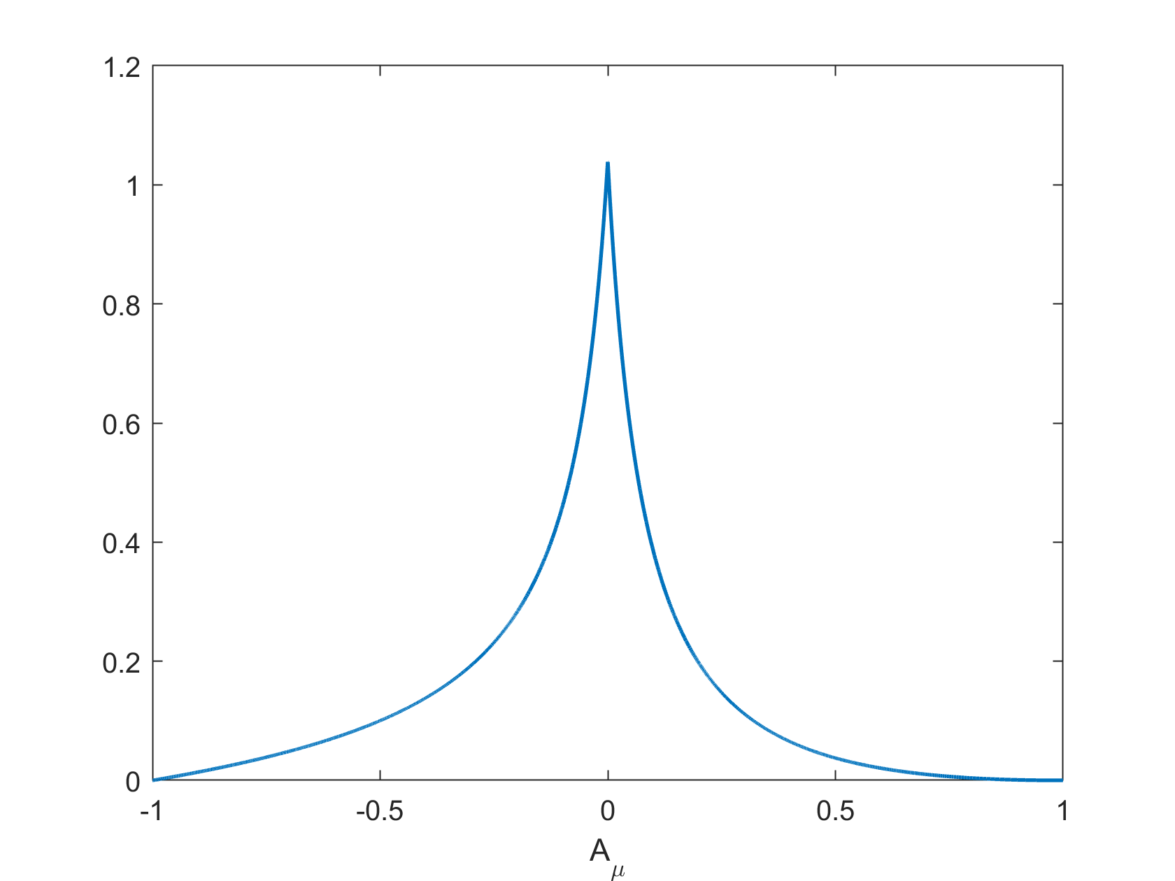
where k⁡(Aμ)>0k(A_{\mu})>0 is defined in (4.9) (see also (4.10) and Figure 1), and that the area enclosed by 𝓧0\boldsymbol{\mathcal{X}}_{0} is π\pi. Then, for any T>0T>0, there exists a unique global strong solution 𝓧⁡(t)\boldsymbol{\mathcal{X}}(t) to the system (1.10) and (1.13), which lies in the space

𝓧∈C⁡([0,T],ℱν1,1)∩C1​((0,T],ℱν0,1)∩L1​([0,T],ℱ˙ν2,1),\boldsymbol{\mathcal{X}}\in C([0,T];\mathcal{F}^{1,1}_{\nu})\cap C^{1}((0,T];\mathcal{F}^{0,1}_{\nu})\cap L^{1}([0,T];\dot{\mathcal{F}}^{2,1}_{\nu}),

with ν⁡(t)\nu(t) given by (1.27). In particular, it becomes instantaneously analytic. Moreover, the following energy inequality is satisfied for 0≤t≤T0\leq t\leq T:

(1.30) ‖𝑿‖ℱ˙ν1,1​(t)+Ae4​𝒞​∫0t‖𝑿‖ℱ˙ν2,1​(τ)​𝑑τ≤‖𝑿0‖ℱ˙1,1,\|\boldsymbol{X}\|_{\dot{\mathcal{F}}^{1,1}_{\nu}}(t)+\frac{A_{e}}{4}\mathcal{C}\int_{0}^{t}\|\boldsymbol{X}\|_{\dot{\mathcal{F}}^{2,1}_{\nu}}(\tau)d\tau\leq\|\boldsymbol{X}_{0}\|_{\dot{\mathcal{F}}^{1,1}},

with 𝒞=𝒞⁡(‖𝐗0‖ℱ˙1,1,Aμ,νm)>0\mathcal{C}=\mathcal{C}\big(\|\boldsymbol{X}_{0}\|_{\dot{\mathcal{F}}^{1,1}},A_{\mu},\nu_{m}\big)>0 defined in (4.12). In addition,

(1.31) ‖𝑿‖ℱ˙ν1,1​(t)≤‖𝑿0‖ℱ˙1,1​e−Ae4​𝒞​t.\displaystyle\|\boldsymbol{X}\|_{\dot{\mathcal{F}}^{1,1}_{\nu}}(t)\leq\|\boldsymbol{X}_{0}\|_{\dot{\mathcal{F}}^{1,1}}e^{-\frac{A_{e}}{4}\mathcal{C}t}.

The zero frequency 𝐗c^​(0)\widehat{\boldsymbol{X}_{c}}(0) remains uniformly bounded for all times as follows

|𝑿c^​(0)|≤|𝑿^0,c​(0)|+C~​‖𝑿0‖ℱ˙1,12,|\widehat{\boldsymbol{X}_{c}}(0)|\leq|\widehat{\boldsymbol{X}}_{0,c}(0)|+\tilde{C}\|\boldsymbol{X}_{0}\|_{\dot{\mathcal{F}}^{1,1}}^{2},

with C~=C~​(‖𝐗0‖ℱ˙1,1,Aμ)>0\tilde{C}=\tilde{C}\big(\|\boldsymbol{X}_{0}\|_{\dot{\mathcal{F}}^{1,1}},A_{\mu}\big)>0 given in (4.15), while

(1.32) 1−12​‖𝑿‖ℱ˙ν1,12≤|𝑿^c​(1)|2≤1+12​‖𝑿‖ℱ˙ν1,12.1-\frac{1}{2}\|\boldsymbol{X}\|_{\dot{\mathcal{F}}^{1,1}_{\nu}}^{2}\leq|\widehat{\boldsymbol{X}}_{c}(1)|^{2}\leq 1+\frac{1}{2}\|\boldsymbol{X}\|_{\dot{\mathcal{F}}^{1,1}_{\nu}}^{2}.

We remark that the decay to zero of the deviation 𝑿\boldsymbol{X} in (1.31) together with (1.32) shows the exponentially fast convergence to a uniformly parametrized circle with the same area as the initial one.
Refer to caption
Figure 1. 103​k​(Aμ)10^{3}k(A_{\mu})
Remark 1.3.

In our results, we assume that both viscosities μ1\mu_{1} and μ2\mu_{2} are positive and hence −1<Aμ<1-1<A_{\mu}<1. We remark on the endpoint cases of Aμ=±1A_{\mu}=\pm 1, which formally correspond to the cases when μ1=0\mu_{1}=0 or μ2=0\mu_{2}=0. As can be seen from Fig. 1, the allowed size of the deviation from 𝐗0\boldsymbol{X}_{0} tends to 00 as Aμ→±1A_{\mu}\to\pm 1, which may indicate potential difficulties in formulating a well-posed mathematical problem for the endpoint cases. From a physical standpoint, it does not make sense to set the viscosity to 00 in either Ω1\Omega_{1} or Ω2\Omega_{2}, and thus a proper treatment of these endpoint cases will require a rethinking of the physical situation under consideration. The case Aμ=−1A_{\mu}=-1 or μ2=0\mu_{2}=0 may be thought of as corresponding to the problem in which a droplet of Stokesian fluid is floating in vacuum. One significant difference between this and the Peskin problem is that in the former problem a droplet in linear translation or rigid rotation experiences no external forces. The force balance and continuity equations will thus have to be supplemented by auxiliary conditions that assure uniqueness, after which this problem is likely to be well-posed. In the case Aμ=1A_{\mu}=1 or μ1=0\mu_{1}=0, Ω1\Omega_{1} might be considered to be vacuum. It is not clear if this problem is well-posed. We will not pursue these issues further.

1.5. Outline

The rest of the paper is structured as follows. In Section 2, we first decompose in 2.1 the system (1.10), (1.13) into zero order, linear, and nonlinear parts around the equilibrium configuration, and then in Section 2.2 we perform the linearization of the problem and show its parabolic structure. Section 2.3 shows how this structure leads to dissipation and in Section 2.4 we summarize the system of equations in its final form. Section 3 contains the crucial nonlinear estimates needed to prove Theorem 1.2. Finally, Section 4 is dedicated to the proof of Theorem 1.2 via a regularization argument and also shows the uniqueness of the solutions.

2. Linearization around the steady state

We will linearize the system (1.9)-(1.15), with 𝑭el\boldsymbol{F}_{\text{el}} given by (1.7), around a time-dependent uniformly parametrized circle with center (c⁡(t),d⁡(t))(c(t),d(t)) and radius R⁡(t)R(t):

(2.1) 𝑿c​(θ,t)=a⁡(t)​𝒆𝒓​(θ)+b⁡(t)​𝒆𝒕​(θ)+c⁡(t)​𝒆𝟏+d⁡(t)​𝒆𝟐,\boldsymbol{X}_{c}(\theta,t)=a(t)\boldsymbol{e_{r}}(\theta)+b(t)\boldsymbol{e_{t}}(\theta)+c(t)\boldsymbol{e_{1}}+d(t)\boldsymbol{e_{2}},
R2​(t)=a2​(t)+b2​(t),R^{2}(t)=a^{2}(t)+b^{2}(t),

where a⁡(t)a(t), b⁡(t)b(t), c⁡(t)c(t) and d⁡(t)d(t) are arbitrary time dependent functions and 𝒆𝒓​(θ)\boldsymbol{e_{r}}(\theta), 𝒆𝒕​(θ)\boldsymbol{e_{t}}(\theta), 𝒆𝟏​(θ)\boldsymbol{e_{1}}(\theta), 𝒆𝟐​(θ)\boldsymbol{e_{2}}(\theta) are defined in (1.16). For notational convenience, we will suppress the time dependence of the coefficients.

2.1. Nonlinear Expansion

We will denote by 𝑿⁡(θ)\boldsymbol{X}(\theta) the deviation from the circle 𝑿c​(θ)\boldsymbol{X}_{c}(\theta) as 𝑿⁡(θ)=𝓧⁡(θ)−𝑿c​(θ)\boldsymbol{X}(\theta)=\boldsymbol{\mathcal{X}}(\theta)-\boldsymbol{X}_{c}(\theta). We define further

Δ​𝑿​=def​𝑿​(θ)−𝑿⁡(η),\Delta\boldsymbol{X}\overset{\mbox{\tiny{def}}}{=}\boldsymbol{X}(\theta)-\boldsymbol{X}(\eta),

and

(2.2) Δη​𝑿​(θ)​=def​𝑿⁡(θ)−𝑿⁡(η)2​sin⁡(θ−η2).\Delta_{\eta}\boldsymbol{X}(\theta)\overset{\mbox{\tiny{def}}}{=}\frac{\boldsymbol{X}(\theta)-\boldsymbol{X}(\eta)}{2\sin{\left(\frac{\theta-\eta}{2}\right)}}.

In particular, we have

Δη​𝑿c​(θ)=a​𝒆𝒕​(θ+η2)−b​𝒆𝒓​(θ+η2),\Delta_{\eta}\boldsymbol{X}_{c}(\theta)=a\hskip 1.42271pt\boldsymbol{e_{t}}\Big(\frac{\theta\!+\!\eta}{2}\Big)-b\hskip 1.42271pt\boldsymbol{e_{r}}\Big(\frac{\theta\!+\!\eta}{2}\Big),

since

Δη​𝒆𝒓​(θ)\displaystyle\Delta_{\eta}\boldsymbol{e_{r}}(\theta) =[−sin⁡(θ+η2)cos⁡(θ+η2)]=𝒆𝒕​(θ+η2),\displaystyle=\begin{bmatrix}-\sin{\left(\frac{\theta+\eta}{2}\right)}\\ \cos{\left(\frac{\theta+\eta}{2}\right)}\end{bmatrix}\!=\boldsymbol{e_{t}}\Big(\frac{\theta\!+\!\eta}{2}\Big),
Δη​𝒆𝒕​(θ)\displaystyle\Delta_{\eta}\boldsymbol{e_{t}}(\theta) =[−cos⁡(θ+η2)−sin⁡(θ+η2)]=−𝒆𝒓​(θ+η2),\displaystyle=\begin{bmatrix}-\cos{\left(\frac{\theta+\eta}{2}\right)}\\ -\sin{\left(\frac{\theta+\eta}{2}\right)}\end{bmatrix}\!=-\boldsymbol{e_{r}}\Big(\frac{\theta\!+\!\eta}{2}\Big),

where we have used the trigonometric identities

sin⁡(θ)−sin⁡(η)\displaystyle\sin{(\theta)}-\sin{(\eta)} =2​sin⁡(θ−η2)​cos⁡(θ+η2),\displaystyle=2\sin{\Big(\frac{\theta-\eta}{2}\Big)}\cos{\Big(\frac{\theta+\eta}{2}\Big)},
cos⁡(θ)−cos⁡(η)\displaystyle\cos{(\theta)}-\cos{(\eta)} =−2​sin⁡(θ−η2)​sin⁡(θ+η2).\displaystyle=-2\sin{\Big(\frac{\theta-\eta}{2}\Big)}\sin{\Big(\frac{\theta+\eta}{2}\Big)}.

Recalling (2.1) and using the identities

∂θ𝒆𝒓​(θ)\displaystyle\partial_{\theta}\boldsymbol{e_{r}}(\theta) =𝒆𝒓​(θ)⟂=𝒆𝒕​(θ),\displaystyle=\boldsymbol{e_{r}}(\theta)^{\perp}=\boldsymbol{e_{t}}(\theta),
∂θ𝒆𝒕​(θ)\displaystyle\partial_{\theta}\boldsymbol{e_{t}}(\theta) =𝒆𝒕​(θ)⟂=−𝒆𝒓​(θ),\displaystyle=\boldsymbol{e_{t}}(\theta)^{\perp}=-\boldsymbol{e_{r}}(\theta),

one has that

∂θ𝑿c​(θ)\displaystyle\partial_{\theta}\boldsymbol{X}_{c}(\theta) =a​𝒆𝒕​(θ)−b​𝒆𝒓​(θ),\displaystyle=a\boldsymbol{e_{t}}(\theta)-b\boldsymbol{e_{r}}(\theta),
∂θ𝑿c​(θ)⟂\displaystyle\partial_{\theta}\boldsymbol{X}_{c}(\theta)^{\perp} =−a​𝒆𝒓​(θ)−b​𝒆𝒕​(θ).\displaystyle=-a\boldsymbol{e_{r}}(\theta)-b\boldsymbol{e_{t}}(\theta).

The trigonometric identities cos⁡(a+b)=cos⁡(a)​cos⁡(b)−sin⁡(a)​sin⁡(b)\cos(a+b)=\cos(a)\cos(b)-\sin(a)\sin(b) and sin⁡(a+b)=sin⁡(a)​cos⁡(b)−cos⁡(a)​sin⁡(b)\sin(a+b)=\sin(a)\cos(b)-\cos(a)\sin(b) further give that

𝒆𝒓​(θ)⋅𝒆𝒕​(θ+η2)\displaystyle\boldsymbol{e_{r}}(\theta)\cdot\boldsymbol{e_{t}}\Big(\frac{\theta+\eta}{2}\Big) =sin⁡(θ−η2),\displaystyle=\sin{\Big(\frac{\theta-\eta}{2}\Big)},
𝒆𝒓​(θ)⋅𝒆𝒓​(θ+η2)\displaystyle\boldsymbol{e_{r}}(\theta)\cdot\boldsymbol{e_{r}}\Big(\frac{\theta+\eta}{2}\Big) =cos⁡(θ−η2),\displaystyle=\cos{\Big(\frac{\theta-\eta}{2}\Big)},
𝒆𝒕​(θ)⋅𝒆𝒕​(θ+η2)\displaystyle\boldsymbol{e_{t}}(\theta)\cdot\boldsymbol{e_{t}}\Big(\frac{\theta+\eta}{2}\Big) =cos⁡(θ−η2),\displaystyle=\cos{\Big(\frac{\theta-\eta}{2}\Big)},
𝒆𝒕​(θ)⋅𝒆𝒓​(θ+η2)\displaystyle\boldsymbol{e_{t}}(\theta)\cdot\boldsymbol{e_{r}}\Big(\frac{\theta+\eta}{2}\Big) =−sin⁡(θ−η2).\displaystyle=-\sin{\Big(\frac{\theta-\eta}{2}\Big)}.

These calculations imply the following computations for a circle that will be used frequently throughout the paper

(2.3) ∂θ𝑿c​(θ)⟂⋅Δη​𝑿c​(θ)=−R2​sin⁡(θ−η2),\partial_{\theta}\boldsymbol{X}_{c}(\theta)^{\perp}\cdot\Delta_{\eta}\boldsymbol{X}_{c}(\theta)=-R^{2}\sin{\Big(\frac{\theta-\eta}{2}\Big)},
(2.4) ∂θ𝑿c​(θ)⋅Δη​𝑿c​(θ)=R2​cos⁡(θ−η2),\partial_{\theta}\boldsymbol{X}_{c}(\theta)\cdot\Delta_{\eta}\boldsymbol{X}_{c}(\theta)=R^{2}\cos{\Big(\frac{\theta-\eta}{2}\Big)},
(2.5) Δη​𝑿c​(θ)⊗Δη​𝑿c​(θ)=a22​[1−cos⁡(θ+η)−sin⁡(θ+η)−sin⁡(θ+η)1+cos⁡(θ+η)]+b22​[+cos⁡(θ+η)sin⁡(θ+η)sin⁡(θ+η)−cos⁡(θ+η)]+a​b​[sin⁡(θ+η)−cos⁡(θ+η)−cos⁡(θ+η)−sin⁡(θ+η)].\Delta_{\eta}\boldsymbol{X}_{c}(\theta)\otimes\Delta_{\eta}\boldsymbol{X}_{c}(\theta)=\frac{a^{2}}{2}\begin{bmatrix}1-\cos{(\theta+\eta)}&-\sin{(\theta+\eta)}\\ -\sin{(\theta+\eta)}&1+\cos{(\theta+\eta)}\end{bmatrix}\\ +\frac{b^{2}}{2}\begin{bmatrix}1\!+\!\cos{(\theta\!+\!\eta)}&\sin{(\theta\!+\!\eta)}\\ \sin{(\theta\!+\!\eta)}&1\!-\!\cos{(\theta\!+\!\eta)}\end{bmatrix}\!+\!ab\begin{bmatrix}\sin{(\theta\!+\!\eta)}&\!-\!\cos{(\theta\!+\!\eta)}\\ -\cos{(\theta\!+\!\eta)}&\!-\!\sin{(\theta\!+\!\eta)}\end{bmatrix}.

The matrices in the last line above have been simplified using the identities sin2⁡(a)=1−cos⁡(2​a)2\sin^{2}(a)=\frac{1-\cos(2a)}{2}, cos2⁡(a)=1+cos⁡(2​a)2\cos^{2}(a)=\frac{1+\cos(2a)}{2}, and sin⁡(2​a)=2​sin⁡(a)​cos⁡(a)\sin(2a)=2\sin(a)\cos(a).

Next, we perform a Taylor expansion of the nonlinear terms around the a time-dependent uniformly parametrized circle (2.1) under the assumption that |Δη​𝑿​(θ)|<1|\Delta_{\eta}\boldsymbol{X}(\theta)|<1. First, we start with the magnitude of the curve

|Δ𝑿+Δ𝑿c|2=4R2sin2(θ−η2)(+2R2Δη𝑿c(θ)⋅Δη𝑿(θ)+1R2|Δη𝑿(θ)|2).\displaystyle|\Delta\boldsymbol{X}\!+\!\Delta\boldsymbol{X}_{c}|^{2}\!=\!4R^{2}\sin^{2}{\left(\frac{\theta\!-\!\eta}{2}\right)}\Big(1\!+\!\frac{2}{R^{2}}\Delta_{\eta}\boldsymbol{X}_{c}(\theta)\cdot\Delta_{\eta}\boldsymbol{X}(\theta)\!+\!\frac{1}{R^{2}}|\Delta_{\eta}\boldsymbol{X}(\theta)|^{2}\Big).

Recalling the expression for G⁡(Δ​𝓧)G(\Delta\boldsymbol{\mathcal{X}}) in (1.9), we expand each term

(2.6) log⁡|Δ​𝑿+Δ​𝑿c|\displaystyle\log{|\Delta\boldsymbol{X}\!+\!\Delta\boldsymbol{X}_{c}|} =log⁡(2​R​|sin⁡(θ−η2)|)\displaystyle=\!\log{\!\left(\!2R\left|\sin{\!\left(\!\frac{\theta\!-\!\eta}{2}\right)}\!\right|\right)}
+12log(+2R2Δη𝑿c(θ)⋅Δη𝑿(θ)+1R2|Δη𝑿(θ)|2)\displaystyle+\!\frac{1}{2}\log{\!\big(1\!+\!\frac{2}{R^{2}}\Delta_{\eta}\boldsymbol{X}_{c}(\theta)\!\cdot\!\Delta_{\eta}\boldsymbol{X}(\theta)\!+\!\frac{1}{R^{2}}|\Delta_{\eta}\boldsymbol{X}(\theta)|^{2}\big)}
=log⁡(2​R​|sin⁡(θ−η2)|)+1R2​Δη​𝑿c​(θ)⋅Δη​𝑿​(θ)+ℛ1​(Δη​𝑿​(θ)),\displaystyle=\log{\left(\!2R\left|\sin\!{\left(\frac{\theta\!-\!\eta}{2}\right)}\right|\right)}\!+\frac{1}{R^{2}}\Delta_{\eta}\boldsymbol{X}_{c}(\theta)\!\cdot\!\Delta_{\eta}\boldsymbol{X}(\theta)\!+\!\mathcal{R}_{1}(\Delta_{\eta}\boldsymbol{X}(\theta)),

where

(2.7) ℛ1​(Δη​𝑿​(θ))=∑n=1∞∑m=0n+m≥2n(nm)​(−1)n−12​n​R2​n​(2​Δη​𝑿c​(θ)⋅Δη​𝑿​(θ))n−m​|Δη​𝑿​(θ)|2​m.\mathcal{R}_{1}(\Delta_{\eta}\boldsymbol{X}(\theta))\!=\!\!\sum_{n=1}^{\infty}\!\!\!\sum_{\begin{subarray}{c}m=0\\ n+m\geq 2\end{subarray}}^{n}\!\!\!\!\!\begin{pmatrix}n\\ m\end{pmatrix}\!\!\frac{(-1)^{n-1}}{2nR^{2n}}(2\Delta_{\eta}\boldsymbol{X}_{c}(\theta)\cdot\Delta_{\eta}\boldsymbol{X}(\theta))^{n-m}|\Delta_{\eta}\boldsymbol{X}(\theta)|^{2m}.

We expand the denominator in the second term of (1.9) as

(2.8) 1|Δ​𝑿+Δ​𝑿c|2=14​R2​sin2⁡(θ−η2)(−2R2Δη𝑿c(θ)⋅Δη𝑿(θ))+14​R2​sin2⁡(θ−η2)​ℛ2​(Δη​𝑿​(θ)),\frac{1}{|\Delta\boldsymbol{X}+\Delta\boldsymbol{X}_{c}|^{2}}=\frac{1}{4R^{2}\sin^{2}{\left(\frac{\theta-\eta}{2}\right)}}\Big(1\!-\!\frac{2}{R^{2}}\Delta_{\eta}\boldsymbol{X}_{c}(\theta)\cdot\Delta_{\eta}\boldsymbol{X}(\theta)\Big)\\ +\frac{1}{4R^{2}\sin^{2}{\left(\frac{\theta-\eta}{2}\right)}}\mathcal{R}_{2}(\Delta_{\eta}\boldsymbol{X}(\theta)),

with the notation

(2.9) ℛ2​(Δη​𝑿​(θ))=∑n=1∞∑m=0n+m≥2n(nm)​(−1)nR2​n​(2​Δη​𝑿c​(θ)⋅Δη​𝑿​(θ))n−m​|Δη​𝑿​(θ)|2​m.\mathcal{R}_{2}(\Delta_{\eta}\boldsymbol{X}(\theta))=\!\sum_{n=1}^{\infty}\!\!\sum_{\begin{subarray}{c}m=0\\ n+m\geq 2\end{subarray}}^{n}\!\!\!\begin{pmatrix}n\\ m\end{pmatrix}\!\frac{(-1)^{n}}{R^{2n}}(2\Delta_{\eta}\boldsymbol{X}_{c}(\theta)\cdot\Delta_{\eta}\boldsymbol{X}(\theta))^{n-m}|\Delta_{\eta}\boldsymbol{X}(\theta)|^{2m}.

Therefore, we can write

(2.10) (Δ​𝑿+Δ​𝑿c)⊗(Δ​𝑿+Δ​𝑿c)|Δ​𝑿+Δ​𝑿c|2=A0+AL+AN,\displaystyle\frac{(\Delta\boldsymbol{X}+\Delta\boldsymbol{X}_{c})\otimes(\Delta\boldsymbol{X}+\Delta\boldsymbol{X}_{c})}{|\Delta\boldsymbol{X}+\Delta\boldsymbol{X}_{c}|^{2}}=A_{0}+A_{L}+A_{N},

with

A0\displaystyle A_{0} =1R2​Δη​𝑿c​(θ)⊗Δη​𝑿c​(θ),\displaystyle=\frac{1}{R^{2}}\Delta_{\eta}\boldsymbol{X}_{c}(\theta)\otimes\Delta_{\eta}\boldsymbol{X}_{c}(\theta),
AL\displaystyle A_{L} =−2R4Δη𝑿c(θ)⋅Δη𝑿(θ)Δη𝑿c(θ)⊗Δη𝑿c(θ)+1R2Δη𝑿c(θ)⊗Δη𝑿(θ)\displaystyle=-\frac{2}{R^{4}}\Delta_{\eta}\boldsymbol{X}_{c}(\theta)\cdot\Delta_{\eta}\boldsymbol{X}(\theta)\Delta_{\eta}\boldsymbol{X}_{c}(\theta)\otimes\Delta_{\eta}\boldsymbol{X}_{c}(\theta)+\frac{1}{R^{2}}\Delta_{\eta}\boldsymbol{X}_{c}(\theta)\otimes\Delta_{\eta}\boldsymbol{X}(\theta)
+1R2Δη𝑿(θ)⊗Δη𝑿c(θ),\displaystyle+\frac{1}{R^{2}}\Delta_{\eta}\boldsymbol{X}(\theta)\otimes\Delta_{\eta}\boldsymbol{X}_{c}(\theta),

and the nonlinear term is given by

AN\displaystyle A_{N} =1R2​Δη​𝑿​(θ)⊗Δη​𝑿​(θ)​(1−2R2​Δη​𝑿c​(θ)⋅Δη​𝑿​(θ)+ℛ2​(Δη​𝑿​(θ)))\displaystyle=\frac{1}{R^{2}}\Delta_{\eta}\boldsymbol{X}(\theta)\otimes\Delta_{\eta}\boldsymbol{X}(\theta)\left(1-\frac{2}{R^{2}}\Delta_{\eta}\boldsymbol{X}_{c}(\theta)\cdot\Delta_{\eta}\boldsymbol{X}(\theta)+\mathcal{R}_{2}(\Delta_{\eta}\boldsymbol{X}(\theta))\right)
+1R2Δη𝑿c(θ)⊗Δη𝑿(θ)(−2R2Δη𝑿c(θ)⋅Δη𝑿(θ)+ℛ2(Δη𝑿(θ)))\displaystyle+\frac{1}{R^{2}}\Delta_{\eta}\boldsymbol{X}_{c}(\theta)\!\otimes\!\Delta_{\eta}\boldsymbol{X}(\theta)\!\left(\!\!-\!\frac{2}{R^{2}}\Delta_{\eta}\boldsymbol{X}_{c}(\theta)\!\cdot\!\Delta_{\eta}\boldsymbol{X}(\theta)\!+\!\mathcal{R}_{2}(\Delta_{\eta}\boldsymbol{X}(\theta))\right)
+1R2Δη𝑿(θ)⊗Δη𝑿c(θ)(−2R2Δη𝑿c(θ)⋅Δη𝑿(θ)+ℛ2(Δη𝑿(θ)))\displaystyle+\frac{1}{R^{2}}\Delta_{\eta}\boldsymbol{X}(\theta)\!\otimes\!\Delta_{\eta}\boldsymbol{X}_{c}(\theta)\!\left(\!\!-\!\frac{2}{R^{2}}\Delta_{\eta}\boldsymbol{X}_{c}(\theta)\!\cdot\!\Delta_{\eta}\boldsymbol{X}(\theta)\!+\!\mathcal{R}_{2}(\Delta_{\eta}\boldsymbol{X}(\theta))\right)
+1R2Δη𝑿c(θ)⊗Δη𝑿c(θ)ℛ2(Δη𝑿(θ)).\displaystyle+\frac{1}{R^{2}}\Delta_{\eta}\boldsymbol{X}_{c}(\theta)\otimes\Delta_{\eta}\boldsymbol{X}_{c}(\theta)\mathcal{R}_{2}(\Delta_{\eta}\boldsymbol{X}(\theta)).

Joining the expansions (2.6) and (2.10), we split G⁡(Δ​𝓧)G(\Delta\boldsymbol{\mathcal{X}}) in (1.9) into zero order, linear, and nonlinear parts in terms of 𝑿\boldsymbol{X} as follows

(2.11) G⁡(Δ​𝓧)=G0​(Δη​𝑿c​(θ))+GL​(Δη​𝑿c​(θ),Δη​𝑿​(θ))+GN​(Δη​𝑿c​(θ),Δη​𝑿​(θ)),G(\Delta\boldsymbol{\mathcal{X}})\\ =G_{0}(\Delta_{\eta}\boldsymbol{X}_{c}(\theta))+G_{L}(\Delta_{\eta}\boldsymbol{X}_{c}(\theta),\Delta_{\eta}\boldsymbol{X}(\theta))+G_{N}(\Delta_{\eta}\boldsymbol{X}_{c}(\theta),\Delta_{\eta}\boldsymbol{X}(\theta)),

where

(2.12) G0​(Δη​𝑿c​(θ))=14​π​(−log⁡(2​R​|sin⁡(θ−η2)|)​I+1R2​Δη​𝑿c​(θ)⊗Δη​𝑿c​(θ)),G_{0}(\Delta_{\eta}\boldsymbol{X}_{c}(\theta))\\ =\frac{1}{4\pi}\left(-\log{\left(2R\left|\sin{\left(\frac{\theta-\eta}{2}\right)}\right|\right)}I+\frac{1}{R^{2}}\Delta_{\eta}\boldsymbol{X}_{c}(\theta)\otimes\Delta_{\eta}\boldsymbol{X}_{c}(\theta)\right),
(2.13) GL​(Δη​𝑿c​(θ),Δη​𝑿​(θ))\displaystyle G_{L}(\Delta_{\eta}\boldsymbol{X}_{c}(\theta),\Delta_{\eta}\boldsymbol{X}(\theta)) =14​π​R2(−Δη𝑿c(θ)⋅Δη𝑿(θ)I\displaystyle=\frac{1}{4\pi R^{2}}\Big(\!-\!\Delta_{\eta}\boldsymbol{X}_{c}(\theta)\!\cdot\!\Delta_{\eta}\boldsymbol{X}(\theta)I\!
−2R2Δη𝑿c(θ)⋅Δη𝑿(θ)Δη𝑿c(θ)⊗Δη𝑿c(θ)\displaystyle-\!\frac{2}{R^{2}}\Delta_{\eta}\boldsymbol{X}_{c}(\theta)\!\cdot\!\Delta_{\eta}\boldsymbol{X}(\theta)\Delta_{\eta}\boldsymbol{X}_{c}(\theta)\!\otimes\!\Delta_{\eta}\boldsymbol{X}_{c}(\theta)
+Δη𝑿c(θ)⊗Δη𝑿(θ)+Δη𝑿(θ)⊗Δη𝑿c(θ)),\displaystyle+\Delta_{\eta}\boldsymbol{X}_{c}(\theta)\otimes\Delta_{\eta}\boldsymbol{X}(\theta)+\Delta_{\eta}\boldsymbol{X}(\theta)\otimes\Delta_{\eta}\boldsymbol{X}_{c}(\theta)\Big),
(2.14) GN​(Δη​𝑿c​(θ),Δη​𝑿​(θ))=−14​π​ℛ1​(Δη​𝑿​(θ))​I+14​π​R2Δη𝑿(θ)⊗Δη𝑿(θ)(1−2R2Δη𝑿c(θ)⋅Δη𝑿(θ)+ℛ2(Δη𝑿(θ)))+14​π​R2​(Δη​𝑿c​(θ)⊗Δη​𝑿​(θ)+Δη​𝑿​(θ)⊗Δη​𝑿c​(θ))×(−2R2Δη𝑿c(θ)⋅Δη𝑿(θ)+ℛ2(Δη𝑿(θ)))+14​π​R2Δη𝑿c(θ)⊗Δη𝑿c(θ)ℛ2(Δη𝑿(θ)).G_{N}(\Delta_{\eta}\boldsymbol{X}_{c}(\theta),\Delta_{\eta}\boldsymbol{X}(\theta))=\frac{-1}{4\pi}\mathcal{R}_{1}(\Delta_{\eta}\boldsymbol{X}(\theta))I\\ +\frac{1}{4\pi R^{2}}\Delta_{\eta}\boldsymbol{X}(\theta)\otimes\Delta_{\eta}\boldsymbol{X}(\theta)\Big(1-\frac{2}{R^{2}}\Delta_{\eta}\boldsymbol{X}_{c}(\theta)\cdot\Delta_{\eta}\boldsymbol{X}(\theta)+\mathcal{R}_{2}(\Delta_{\eta}\boldsymbol{X}(\theta))\Big)\\ +\frac{1}{4\pi R^{2}}\Big(\Delta_{\eta}\boldsymbol{X}_{c}(\theta)\otimes\Delta_{\eta}\boldsymbol{X}(\theta)+\Delta_{\eta}\boldsymbol{X}(\theta)\otimes\Delta_{\eta}\boldsymbol{X}_{c}(\theta)\Big)\\ \quad\times\big(-\frac{2}{R^{2}}\Delta_{\eta}\boldsymbol{X}_{c}(\theta)\cdot\Delta_{\eta}\boldsymbol{X}(\theta)+\mathcal{R}_{2}(\Delta_{\eta}\boldsymbol{X}(\theta))\big)\\ +\frac{1}{4\pi R^{2}}\Delta_{\eta}\boldsymbol{X}_{c}(\theta)\otimes\Delta_{\eta}\boldsymbol{X}_{c}(\theta)\mathcal{R}_{2}(\Delta_{\eta}\boldsymbol{X}(\theta)).

Consider the splitting of the solution 𝐅⁡(θ)\mathbf{F}(\theta) to (1.13) into zero order, linear, and nonlinear parts as

(2.15) 𝑭⁡(θ)=𝑭0​(θ)+𝑭L​(θ)+𝑭N​(θ).\boldsymbol{F}(\theta)=\boldsymbol{F}_{0}(\theta)+\boldsymbol{F}_{L}(\theta)+\boldsymbol{F}_{N}(\theta).

(We will prove bounds for these terms in Section 3.2.) Introducing the splittings (2.11) and (2.15) in (1.10), we obtain that

(2.16) 𝓧t​(θ)\displaystyle\boldsymbol{\mathcal{X}}_{t}(\theta) =𝓞⁡(𝑿c)​(θ)+𝓛⁡(𝑿c,𝑿)​(θ)+𝓝⁡(𝑿c,𝑿)​(θ),\displaystyle=\boldsymbol{\mathcal{O}}(\boldsymbol{X}_{c})(\theta)+\boldsymbol{\mathcal{L}}(\boldsymbol{X}_{c},\boldsymbol{X})(\theta)+\boldsymbol{\mathcal{N}}(\boldsymbol{X}_{c},\boldsymbol{X})(\theta),

where we recall that 𝓧⁡(θ)=𝑿⁡(θ)+𝑿c​(θ)\boldsymbol{\mathcal{X}}(\theta)=\boldsymbol{X}(\theta)+\boldsymbol{X}_{c}(\theta) and we use the notation

𝓞⁡(𝑿c)​(θ)=∫𝕊G0​(Δη​𝑿c​(θ))​𝑭0​(η)​dη,\displaystyle\boldsymbol{\mathcal{O}}(\boldsymbol{X}_{c})(\theta)=\int_{\mathbb{S}}G_{0}(\Delta_{\eta}\boldsymbol{X}_{c}(\theta))\boldsymbol{F}_{0}(\eta)d\eta,
𝓛⁡(𝑿c,𝑿)​(θ)=∫𝕊G0​(Δη​𝑿c​(θ))​𝑭L​(η)​dη+∫𝕊GL​(Δη​𝑿c​(θ),Δη​𝑿​(θ))​𝑭0​(η)​dη,\displaystyle\!\boldsymbol{\mathcal{L}}(\boldsymbol{X}_{c},\boldsymbol{X})(\theta)=\int_{\mathbb{S}}G_{0}(\Delta_{\eta}\boldsymbol{X}_{c}(\theta))\boldsymbol{F}_{L}(\eta)d\eta+\int_{\mathbb{S}}G_{L}(\Delta_{\eta}\boldsymbol{X}_{c}(\theta),\Delta_{\eta}\boldsymbol{X}(\theta))\boldsymbol{F}_{0}(\eta)d\eta,
𝓝​(𝑿c,𝑿)​(θ)\displaystyle\!\boldsymbol{\mathcal{N}}(\boldsymbol{X}_{c},\boldsymbol{X})(\theta) =∫𝕊(GL​(Δη​𝑿𝒄​(θ),Δη​𝑿​(θ))​𝑭L​(η)+GN​(Δη​𝑿c​(θ),Δη​𝑿​(θ))​𝑭0​(η)CLOSE\displaystyle=\!\!\!\int_{\mathbb{S}}\!\!\Big(G_{L}(\Delta_{\eta}\boldsymbol{X_{c}}(\theta),\Delta_{\eta}\boldsymbol{X}(\theta))\boldsymbol{F}_{L}(\eta)\!+\!G_{N}(\Delta_{\eta}\boldsymbol{X}_{c}(\theta),\Delta_{\eta}\boldsymbol{X}(\theta))\boldsymbol{F}_{0}(\eta)
OPEN+GN​(Δη​𝑿c​(θ),Δη​𝑿​(θ))​𝑭L​(η)+G⁡(𝓧⁡(θ)−𝓧⁡(η))​𝑭N​(η))​d​η.\displaystyle+\!G_{N}(\Delta_{\eta}\boldsymbol{X}_{c}(\theta),\Delta_{\eta}\boldsymbol{X}(\theta))\boldsymbol{F}_{L}(\eta)\!+\!G(\boldsymbol{\mathcal{X}}(\theta)\!-\!\boldsymbol{\mathcal{X}}(\eta))\boldsymbol{F}_{N}(\eta)\Big)d\eta.

We have thus expanded the evolution equation (1.10) distinguishing the zero order, linear, and nonlinear in 𝑿\boldsymbol{X} contributions.

2.2. Linearized System

We proceed to show that the linearized system gives rise to a diffusion operator on 𝑿\boldsymbol{X}. Since the linear structure is the same for any uniformly parametrized circle (see [17]), we will use now (2.1) with a=1a=1, b=c=d=0b=c=d=0 and R=1R=1 to simplify the computations, and for clarity of notation we will denote this circle by 𝑿⋆\boldsymbol{X}_{\star}.

We will now linearize equations (1.10) and (1.13). We first determine 𝑭0\boldsymbol{F}_{0}, the value of 𝑭\boldsymbol{F} at the steady state:

(2.17) 0=𝓞⁡(𝑿⋆)​(θ)=∫𝕊G0​(Δη​𝑿⋆​(θ))​𝑭0​(η)​𝑑η,\displaystyle 0=\boldsymbol{\mathcal{O}}(\boldsymbol{X}_{\star})(\theta)=\int_{\mathbb{S}}G_{0}(\Delta_{\eta}\boldsymbol{X}_{\star}(\theta))\boldsymbol{F}_{0}(\eta)d\eta,
(2.18) 𝑭0​(θ)−2​Aμ​𝓢𝟎​(𝑭0,𝑿⋆)​(θ)=2​Ae​𝑭~el,0​(θ),\displaystyle\boldsymbol{F}_{0}(\theta)-2A_{\mu}\boldsymbol{\mathcal{S}_{0}}(\boldsymbol{F}_{0},\boldsymbol{X}_{\star})(\theta)=2A_{e}\boldsymbol{\tilde{F}}_{\text{el},0}(\theta),

where

𝑭~el,0​(θ)=∂θ2𝑿⋆​(θ),\boldsymbol{\tilde{F}}_{\text{el},0}(\theta)=\partial_{\theta}^{2}\boldsymbol{X}_{\star}(\theta),

and

𝓢𝟎​(𝑭0,𝑿⋆)​(θ)=1π​∫𝕊∂θ𝑿⋆⟂⋅Δη​𝑿⋆​(θ)​Δη​𝑿⋆​(θ)​Δη​𝑿⋆​(θ)⋅𝑭0​(η)2​sin⁡(θ−η2)​𝑑η.\boldsymbol{\mathcal{S}_{0}}(\boldsymbol{F}_{0},\boldsymbol{X}_{\star})(\theta)\!=\!\frac{1}{\pi}\int_{\mathbb{S}}\partial_{\theta}\boldsymbol{X}_{\star}^{\perp}\cdot\Delta_{\eta}\boldsymbol{X}_{\star}(\theta)\Delta_{\eta}\boldsymbol{X}_{\star}(\theta)\Delta_{\eta}\boldsymbol{X}_{\star}(\theta)\cdot\frac{\boldsymbol{F}_{0}(\eta)}{2\sin{\Big(\frac{\theta-\eta}{2}\Big)}}d\eta.

Rewriting Δη​𝑿⋆​(θ)​Δη​𝑿⋆​(θ)⋅𝑭0​(η)=Δη​𝑿⋆​(θ)⊗Δη​𝑿⋆​(θ)​𝑭0​(η)\Delta_{\eta}\boldsymbol{X}_{\star}(\theta)\Delta_{\eta}\boldsymbol{X}_{\star}(\theta)\cdot\boldsymbol{F}_{0}(\eta)=\Delta_{\eta}\boldsymbol{X}_{\star}(\theta)\otimes\Delta_{\eta}\boldsymbol{X}_{\star}(\theta)\boldsymbol{F}_{0}(\eta), and recalling the computations (2.3) and (2.5), one finds that

𝓢𝟎​(𝑭0,𝑿⋆)​(θ)=−12​π​∫𝕊M⁡(θ,η)​𝑭0​(η)​𝑑η,\boldsymbol{\mathcal{S}_{0}}(\boldsymbol{F}_{0},\boldsymbol{X}_{\star})(\theta)\!=\!\frac{-1}{2\pi}\int_{\mathbb{S}}M(\theta,\eta)\boldsymbol{F}_{0}(\eta)d\eta,

where from (2.5) we have

(2.19) M⁡(θ,η)=Δη​𝑿⋆​(θ)⊗Δη​𝑿⋆​(θ)=12​[−cos⁡(θ+η)−sin⁡(θ+η)−sin⁡(θ+η)+cos⁡(θ+η)],M(\theta,\eta)\!=\!\Delta_{\eta}\boldsymbol{X}_{\star}(\theta)\!\otimes\!\Delta_{\eta}\boldsymbol{X}_{\star}(\theta)\!=\!\frac{1}{2}\begin{bmatrix}1\!-\!\cos{(\theta\!+\!\eta)}&-\sin{(\theta\!+\!\eta)}\\ -\sin{(\theta\!+\!\eta)}&1\!+\!\cos{(\theta\!+\!\eta)}\end{bmatrix},

and therefore 𝑭0\boldsymbol{F}_{0} is defined by

𝑭0​(θ)+Aμπ​∫𝕊M⁡(θ,η)​𝑭0​(η)​𝑑η=2​Ae​∂θ2𝑿⋆​(θ).\boldsymbol{F}_{0}(\theta)+\frac{A_{\mu}}{\pi}\int_{\mathbb{S}}M(\theta,\eta)\boldsymbol{F}_{0}(\eta)d\eta=2A_{e}\partial_{\theta}^{2}\boldsymbol{X}_{\star}(\theta).

Since ∂θ2𝑿⋆=−𝑿⋆\partial_{\theta}^{2}\boldsymbol{X}_{\star}=-\boldsymbol{X}_{\star} and noting that

1π​∫𝕊M⁡(θ,η)​𝑿⋆​(η)​𝑑η=−𝑿⋆​(θ),\frac{1}{\pi}\int_{\mathbb{S}}M(\theta,\eta)\boldsymbol{X}_{\star}(\eta)d\eta=-\boldsymbol{X}_{\star}(\theta),

it is easily seen that

(2.20) 𝑭0​(θ)=2​Ae1−Aμ​∂θ2𝑿⋆​(θ).\boldsymbol{F}_{0}(\theta)=\frac{2A_{e}}{1-A_{\mu}}\partial_{\theta}^{2}\boldsymbol{X}_{\star}(\theta).

Now, recalling (2.12), it can be checked that (2.20) satisfies in fact (2.17):

4​π​(1−Aμ2​Ae)​∫𝕊G0​(Δη​𝑿⋆​(θ))​𝑭0​(η)​𝑑η=−∫𝕊log(2|sin(θ−η2)|)∂η2𝑿⋆(η)dη+∫𝕊M(θ,η)∂η2𝑿⋆(η)dη,4\pi\left(\frac{1-A_{\mu}}{2A_{e}}\right)\int_{\mathbb{S}}G_{0}(\Delta_{\eta}\boldsymbol{X}_{\star}(\theta))\boldsymbol{F}_{0}(\eta)d\eta\\ =-\int_{\mathbb{S}}\log{\left(2\left|\sin{\left(\frac{\theta-\eta}{2}\right)}\right|\right)}\partial_{\eta}^{2}\boldsymbol{X}_{\star}(\eta)d\eta+\int_{\mathbb{S}}M(\theta,\eta)\partial_{\eta}^{2}\boldsymbol{X}_{\star}(\eta)d\eta,

so integration by parts in the first term yields (2.17).

We now proceed to compute the linear term 𝓛​(𝑿⋆,𝑿)​(θ)\boldsymbol{\mathcal{L}}(\boldsymbol{X}_{\star},\boldsymbol{X})(\theta) in (2.16). For convenience, we write it as follows

(2.21) 𝓛⁡(𝑿⋆,𝑿)​(θ)=∫𝕊G0​(Δη​𝑿⋆)​𝑭L​(η)​𝑑η+∫𝕊(∇G​(Δ​𝑿⋆)​𝑭0​(η))​Δ​𝑿​𝑑η,\boldsymbol{\mathcal{L}}(\boldsymbol{X}_{\star},\boldsymbol{X})(\theta)\!=\!\int_{\mathbb{S}}\!\!G_{0}(\Delta_{\eta}\boldsymbol{X}_{\star})\boldsymbol{F}_{L}(\eta)d\eta+\!\int_{\mathbb{S}}(\nabla G(\Delta\boldsymbol{X}_{\star})\boldsymbol{F}_{0}(\eta))\Delta\boldsymbol{X}d\eta,

where G0G_{0} and GG are defined in (2.12) and (1.9), respectively. To simplify the second integral above, note that:

∂Gi​j∂x1​(Δ​𝑿⋆)​er,j​(η)=∂Gi​1∂x1​(Δ​𝑿⋆)​er,1​(η)+∂Gi​2∂x1​(Δ​𝑿⋆)​er,2​(η)=∂Gi​1∂x1​(Δ​𝑿⋆)​∂ηX⋆,2−∂Gi​2∂x1​(Δ​𝑿⋆)​∂ηX⋆,1=−∂Gi​2∂x2(Δ𝑿⋆)∂ηX⋆,2−∂Gi​2∂x1(Δ𝑿⋆)∂ηX⋆,1=∂ηGi​2​(Δ​𝑿⋆).\begin{split}\frac{\partial G_{ij}}{\partial x_{1}}(\Delta\boldsymbol{X}_{\star})e_{{\rm r},j}(\eta)&=\frac{\partial G_{i1}}{\partial x_{1}}(\Delta\boldsymbol{X}_{\star})e_{\rm r,1}(\eta)+\frac{\partial G_{i2}}{\partial x_{1}}(\Delta\boldsymbol{X}_{\star})e_{\rm r,2}(\eta)\\ &=\frac{\partial G_{i1}}{\partial x_{1}}(\Delta\boldsymbol{X}_{\star})\partial_{\eta}X_{\star,2}-\frac{\partial G_{i2}}{\partial x_{1}}(\Delta\boldsymbol{X}_{\star})\partial_{\eta}X_{\star,1}\\ &=-\frac{\partial G_{i2}}{\partial x_{2}}(\Delta\boldsymbol{X}_{\star})\partial_{\eta}X_{\star,2}-\frac{\partial G_{i2}}{\partial x_{1}}(\Delta\boldsymbol{X}_{\star})\partial_{\eta}X_{\star,1}\\ &=\partial_{\eta}G_{i2}(\Delta\boldsymbol{X}_{\star}).\end{split}

Here er,je_{{\rm r},j} is the jj-th component of the vector ere_{{\rm r}} etc. Further, in the third equality above, we used the fact that the Stokeslet is divergence free:

∂Gi​1∂x1+∂Gi​2∂x2=0.\frac{\partial G_{i1}}{\partial x_{1}}+\frac{\partial G_{i2}}{\partial x_{2}}=0.

Likewise, we have:

∂Gi​j∂x2(Δ𝑿⋆)er,j(η)=−∂ηGi​1(Δ𝑿⋆).\frac{\partial G_{ij}}{\partial x_{2}}(\Delta\boldsymbol{X}_{\star})e_{{\rm r},j}(\eta)=-\partial_{\eta}G_{i1}(\Delta\boldsymbol{X}_{\star}).

We thus have:

∫𝕊(∇G​(Δ​𝑿⋆)​𝑭0​(η))​Δ​𝑿​𝑑η=−2​Ae−Aμ∫𝕊(ℛ−1∂ηG(𝑿⋆(θ)−𝑿⋆(η)))Δ𝑿dη=2​Ae−Aμ​∫𝕊(ℛ−1​G​(𝑿⋆​(θ)−𝑿⋆​(η)))​∂η𝑿⁡(η)​𝑑η=2​Ae−Aμ​∫𝕊G⁡(𝑿⋆​(θ)−𝑿⋆​(η))​(ℛ−1​∂η𝑿⁡(η))​dη.\begin{split}\int_{\mathbb{S}}(\nabla G(\Delta\boldsymbol{X}_{\star})\boldsymbol{F}_{0}(\eta))\Delta\boldsymbol{X}d\eta&=-\frac{2A_{e}}{1\!-\!A_{\mu}}\!\int_{\mathbb{S}}(\mathcal{R}^{-1}\partial_{\eta}G(\boldsymbol{X}_{\star}(\theta)\!-\!\boldsymbol{X}_{\star}(\eta)))\Delta\boldsymbol{X}d\eta\\ &=\frac{2A_{e}}{1\!-\!A_{\mu}}\int_{\mathbb{S}}(\mathcal{R}^{-1}G(\boldsymbol{X}_{\star}(\theta)\!-\!\boldsymbol{X}_{\star}(\eta)))\partial_{\eta}\boldsymbol{X}(\eta)d\eta\\ &=\frac{2A_{e}}{1\!-\!A_{\mu}}\!\int_{\mathbb{S}}G(\boldsymbol{X}_{\star}(\theta)\!-\!\boldsymbol{X}_{\star}(\eta))(\mathcal{R}^{-1}\partial_{\eta}\boldsymbol{X}(\eta))d\eta.\end{split}

Since G⁡(𝑿⋆​(θ)−𝑿⋆​(η))​=def​G0​(Δη​𝑿⋆)G(\boldsymbol{X}_{\star}(\theta)-\boldsymbol{X}_{\star}(\eta))\overset{\mbox{\tiny{def}}}{=}G_{0}(\Delta_{\eta}\boldsymbol{X}_{\star}), then (2.21) simplifies to:

(2.22) 𝓛⁡(𝑿⋆,𝑿)​(θ)=∫𝕊G0​(Δη​𝑿⋆)​(𝑭L​(η)+2​Ae−Aμ​ℛ−1​∂η𝑿)​𝑑η.\boldsymbol{\mathcal{L}}(\boldsymbol{X}_{\star},\boldsymbol{X})(\theta)=\int_{\mathbb{S}}G_{0}(\Delta_{\eta}\boldsymbol{X}_{\star})\left(\boldsymbol{F}_{L}(\eta)+\frac{2A_{e}}{1\!-\!A_{\mu}}\mathcal{R}^{-1}\partial_{\eta}\boldsymbol{X}\right)d\eta.

This is our specification of the linearized operator.

We will now determine 𝑭L\boldsymbol{F}_{L} as in (2.15), that is, the linear part of 𝑭\boldsymbol{F} in (1.13). We find

(2.23) 𝑭L​(θ)+Aμπ​∫𝕊M⁡(θ,η)​𝑭L​(η)​dη=2​Ae​∂θ2𝑿−2​Aμ​(𝑸+𝑺),Qi=−∫𝕊𝒯i​j​k(Δ𝑿⋆)F0,k(η)ℛ−1j​l∂θXl(θ)dη,Si=−∫𝕊∂𝒯i​j​k∂xm(Δ𝑿⋆)Δ𝑿mF0,k(η)ℛ−1j​l∂θX⋆,l(θ)dη.\begin{split}&\boldsymbol{F}_{L}(\theta)+\frac{A_{\mu}}{\pi}\int_{\mathbb{S}}M(\theta,\eta)\boldsymbol{F}_{L}(\eta)d\eta=2A_{e}\partial_{\theta}^{2}\boldsymbol{X}-2A_{\mu}(\boldsymbol{Q}+\boldsymbol{S}),\\ &Q_{i}=-\int_{\mathbb{S}}\mathcal{T}_{ijk}(\Delta\boldsymbol{X}_{\star})F_{0,k}(\eta)\mathcal{R}^{-1}_{jl}\partial_{\theta}X_{l}(\theta)d\eta,\\ &S_{i}=-\int_{\mathbb{S}}\frac{\partial\mathcal{T}_{ijk}}{\partial x_{m}}(\Delta\boldsymbol{X}_{\star})\Delta\boldsymbol{X}_{m}F_{0,k}(\eta)\mathcal{R}^{-1}_{jl}\partial_{\theta}X_{\star,l}(\theta)d\eta.\end{split}

Let us compute 𝑸\boldsymbol{Q}. We start with

−𝒯i​j​k​(Δ​𝑿⋆)​F0,k=−2​Ae1−Aμ​Δ​X⋆,i​Δ​X⋆,j​Δ​X⋆,k​er,k​(η)π​|Δ​𝑿⋆|4=2​Ae1−Aμ​Δ​X⋆,i​Δ​X⋆,j2​π​|Δ​𝑿⋆|2,-\mathcal{T}_{ijk}(\Delta\boldsymbol{X}_{\star})F_{0,k}=-\frac{2A_{e}}{1-A_{\mu}}\frac{\Delta X_{\star,i}\Delta X_{\star,j}\Delta X_{\star,k}e_{{\rm r},k}(\eta)}{\pi\left\lvert\Delta\boldsymbol{X}_{\star}\right\rvert^{4}}=\frac{2A_{e}}{1-A_{\mu}}\frac{\Delta X_{\star,i}\Delta X_{\star,j}}{2\pi\left\lvert\Delta\boldsymbol{X}_{\star}\right\rvert^{2}},

where we used

(2.24) Δ​𝑿⋆⋅𝒆r​(η)|Δ​𝑿⋆|2=−12.\frac{\Delta\boldsymbol{X}_{\star}\cdot\boldsymbol{e}_{\rm r}(\eta)}{\left\lvert\Delta\boldsymbol{X}_{\star}\right\rvert^{2}}=-\frac{1}{2}.

Therefore, we have

𝑸=Ae1−Aμ​1π​∫𝕊Δ​𝑿⋆⊗Δ​𝑿⋆|Δ​𝑿⋆|2​dη​ℛ−1​∂θ𝑿⁡(θ)=Ae1−Aμ​1π​∫𝕊M⁡(θ,η)​dη​ℛ−1​∂θ𝑿⁡(θ)=Ae1−Aμ​ℛ−1​∂θ𝑿⁡(θ),\begin{split}\boldsymbol{Q}&=\frac{A_{e}}{1-A_{\mu}}\frac{1}{\pi}\int_{\mathbb{S}}\frac{\Delta\boldsymbol{X}_{\star}\otimes\Delta\boldsymbol{X}_{\star}}{\left\lvert\Delta\boldsymbol{X}_{\star}\right\rvert^{2}}d\eta\mathcal{R}^{-1}\partial_{\theta}\boldsymbol{X}(\theta)\\ &=\frac{A_{e}}{1-A_{\mu}}\frac{1}{\pi}\int_{\mathbb{S}}M(\theta,\eta)d\eta\mathcal{R}^{-1}\partial_{\theta}\boldsymbol{X}(\theta)=\frac{A_{e}}{1-A_{\mu}}\mathcal{R}^{-1}\partial_{\theta}\boldsymbol{X}(\theta),\end{split}

where we used (2.19) in the second equality. We next compute 𝑺\boldsymbol{S},

−∂𝒯i​j​k∂xm(ΔX⋆)ΔXmF0,k(η)ℛ−1j​l∂θX⋆,l(θ)=−1π​2​Ae1−Aμ​(Δ​Xi​Δ​X⋆,j​Δ​X⋆,k​er,j​(θ)​er,k​(η)|Δ​𝑿⋆|4)−2Ae/π1−Aμ​(Δ​X⋆,i​Δ​Xj​Δ​X⋆,k​er,j​(θ)​er,k​(η)|Δ​𝑿⋆|4+Δ​X⋆,i​Δ​X⋆,j​Δ​Xk​er,j​(θ)​er,k​(η)|Δ​𝑿⋆|4)+8​Ae/π1−Aμ​(Δ​X⋆,i​Δ​X⋆,j​Δ​X⋆,k​er,j​(θ)​er,k​(η)​Δ​X⋆,m​Δ​Xm|Δ​𝑿⋆|6).\begin{split}&-\frac{\partial\mathcal{T}_{ijk}}{\partial x_{m}}(\Delta X_{\star})\Delta X_{m}F_{0,k}(\eta)\mathcal{R}^{-1}_{jl}\partial_{\theta}X_{\star,l}(\theta)\\ =&-\frac{1}{\pi}\frac{2A_{e}}{1-A_{\mu}}\left(\frac{\Delta X_{i}\Delta X_{\star,j}\Delta X_{\star,k}e_{{\rm r},j}(\theta)e_{{\rm r},k}(\eta)}{\left\lvert\Delta\boldsymbol{X}_{\star}\right\rvert^{4}}\right)\\ &\frac{-2A_{e}/\pi}{1-A_{\mu}}\!\!\left(\!\frac{\Delta X_{\star,i}\Delta X_{j}\Delta X_{\star,k}e_{{\rm r},j}(\theta)e_{{\rm r},k}(\eta)}{\left\lvert\Delta\boldsymbol{X}_{\star}\right\rvert^{4}}\!+\!\frac{\Delta X_{\star,i}\Delta X_{\star,j}\Delta X_{k}e_{{\rm r},j}(\theta)e_{{\rm r},k}(\eta)}{\left\lvert\Delta\boldsymbol{X}_{\star}\right\rvert^{4}}\right)\\ &+\frac{8A_{e}/\pi}{1-A_{\mu}}\left(\frac{\Delta X_{\star,i}\Delta X_{\star,j}\Delta X_{\star,k}e_{{\rm r},j}(\theta)e_{{\rm r},k}(\eta)\Delta X_{\star,m}\Delta X_{m}}{\left\lvert\Delta\boldsymbol{X}_{\star}\right\rvert^{6}}\right).\\ \end{split}

We simplify each term as follows

Δ​Xi​Δ​X⋆,j​Δ​X⋆,k​er,j​(θ)​er,k​(η)|Δ​𝑿⋆|4=−14​Δ​Xi,Δ​X⋆,i​Δ​Xj​Δ​X⋆,k​er,j​(θ)​er,k​(η)|Δ​𝑿⋆|4+Δ​X⋆,i​Δ​X⋆,j​Δ​Xk​er,j​(θ)​er,k​(η)|Δ​𝑿⋆|4=−Δ​X⋆,i​Δ​Xj​er,j​(θ)2​|Δ​𝑿⋆|2+Δ​X⋆,i​Δ​Xk​er,k​(η)2​|Δ​𝑿⋆|2=−Δ​X⋆,i​Δ​X⋆,j​Δ​Xj2​|Δ​𝑿⋆|2,Δ​X⋆,i​Δ​X⋆,j​Δ​X⋆,k​er,j​(θ)​er,k​(η)​Δ​X⋆,m​Δ​Xm|Δ​𝑿⋆|6=−Δ​X⋆,i​Δ​X⋆,j​Δ​Xj4​|Δ​𝑿⋆|2,\begin{split}&\frac{\Delta X_{i}\Delta X_{\star,j}\Delta X_{\star,k}e_{{\rm r},j}(\theta)e_{{\rm r},k}(\eta)}{\left\lvert\Delta\boldsymbol{X}_{\star}\right\rvert^{4}}=-\frac{1}{4}\Delta X_{i},\\ &\frac{\Delta X_{\star,i}\Delta X_{j}\Delta X_{\star,k}e_{{\rm r},j}(\theta)e_{{\rm r},k}(\eta)}{\left\lvert\Delta\boldsymbol{X}_{\star}\right\rvert^{4}}+\frac{\Delta X_{\star,i}\Delta X_{\star,j}\Delta X_{k}e_{{\rm r},j}(\theta)e_{{\rm r},k}(\eta)}{\left\lvert\Delta\boldsymbol{X}_{\star}\right\rvert^{4}}\\ &=\frac{-\Delta X_{\star,i}\Delta X_{j}e_{{\rm r},j}(\theta)}{2\left\lvert\Delta\boldsymbol{X}_{\star}\right\rvert^{2}}+\frac{\Delta X_{\star,i}\Delta X_{k}e_{{\rm r},k}(\eta)}{2\left\lvert\Delta\boldsymbol{X}_{\star}\right\rvert^{2}}=-\frac{\Delta X_{\star,i}\Delta X_{\star,j}\Delta X_{j}}{2\left\lvert\Delta\boldsymbol{X}_{\star}\right\rvert^{2}},\\ &\frac{\Delta X_{\star,i}\Delta X_{\star,j}\Delta X_{\star,k}e_{{\rm r},j}(\theta)e_{{\rm r},k}(\eta)\Delta X_{\star,m}\Delta X_{m}}{\left\lvert\Delta\boldsymbol{X}_{\star}\right\rvert^{6}}=-\frac{\Delta X_{\star,i}\Delta X_{\star,j}\Delta X_{j}}{4\left\lvert\Delta\boldsymbol{X}_{\star}\right\rvert^{2}},\end{split}

where above we made repeated use of (2.24) and

Δ𝑿⋆⋅ℛ−1∂θ𝑿⋆(θ)|Δ​𝑿⋆|2=Δ​𝑿⋆⋅er​(θ)|Δ​𝑿⋆|2=12.\frac{\Delta\boldsymbol{X}_{\star}\cdot\mathcal{R}^{-1}\partial_{\theta}\boldsymbol{X}_{\star}(\theta)}{\left\lvert\Delta\boldsymbol{X}_{\star}\right\rvert^{2}}=\frac{\Delta\boldsymbol{X}_{\star}\cdot e_{{\rm r}}(\theta)}{\left\lvert\Delta\boldsymbol{X}_{\star}\right\rvert^{2}}=\frac{1}{2}.

Thus we have

−∂𝒯i​j​k∂xm(ΔX⋆)ΔXmF0,k(η)ℛj​l−1∂θX⋆,l=Ae/2​π1−Aμ(ΔXi−2​Δ​X⋆,i​Δ​X⋆,j​Δ​Xj|Δ​𝑿⋆|2).-\frac{\partial\mathcal{T}_{ijk}}{\partial x_{m}}(\Delta X_{\star})\Delta X_{m}F_{0,k}(\eta)\mathcal{R}^{-1}_{jl}\partial_{\theta}X_{\star,l}=\frac{A_{e}/2\pi}{1-A_{\mu}}\left(\Delta X_{i}-\frac{2\Delta X_{\star,i}\Delta X_{\star,j}\Delta X_{j}}{\left\lvert\Delta\boldsymbol{X}_{\star}\right\rvert^{2}}\right).

Substituting this back into the expression for 𝑺\boldsymbol{S} in (2.23), we have:

𝑺=Ae/2​π1−Aμ∫𝕊(I−2M(θ,η))Δ𝑿dη=−Ae/2​π1−Aμ∫𝕊(I−2M(θ,η))𝑿(η)dη=Ae/2​π1−Aμ​(−⟨𝒆r,𝑿⟩​𝒆r+⟨𝒆t,𝑿⟩​𝒆t),\begin{split}\boldsymbol{S}&=\frac{A_{e}/2\pi}{1-A_{\mu}}\int_{\mathbb{S}}(I-2M(\theta,\eta))\Delta\boldsymbol{X}d\eta=-\frac{A_{e}/2\pi}{1-A_{\mu}}\int_{\mathbb{S}}(I-2M(\theta,\eta))\boldsymbol{X}(\eta)d\eta\\ &=\frac{A_{e}/2\pi}{1-A_{\mu}}\left(-\left\langle\boldsymbol{e}_{\rm r},\boldsymbol{X}\right\rangle\boldsymbol{e}_{\rm r}+\left\langle\boldsymbol{e}_{\rm t},\boldsymbol{X}\right\rangle\boldsymbol{e}_{\rm t}\right),\end{split}

where we used (2.19) in the first equality and we are using the notation (1.24) for the inner product.

Equation (2.23) thus reduces to:

𝑭L​(θ)+Aμπ​∫𝕊M⁡(θ,η)​𝑭L​(η)​𝑑η=2​Ae​∂θ2𝑿⁡(θ)−2​Ae​Aμ1−Aμ​(ℛ−1​∂θ𝑿⁡(θ)+12​π​(−⟨𝒆r,𝑿⟩​𝒆r​(θ)+⟨𝒆t,𝑿⟩​𝒆t​(θ))).\begin{split}&\boldsymbol{F}_{L}(\theta)+\frac{A_{\mu}}{\pi}\int_{\mathbb{S}}M(\theta,\eta)\boldsymbol{F}_{L}(\eta)d\eta\\ =&2A_{e}\partial_{\theta}^{2}\boldsymbol{X}(\theta)-\frac{2A_{e}A_{\mu}}{1-A_{\mu}}\left(\mathcal{R}^{-1}\partial_{\theta}\boldsymbol{X}(\theta)+\frac{1}{2\pi}\left(-\left\langle\boldsymbol{e}_{\rm r},\boldsymbol{X}\right\rangle\boldsymbol{e}_{\rm r}(\theta)+\left\langle\boldsymbol{e}_{\rm t},\boldsymbol{X}\right\rangle\boldsymbol{e}_{\rm t}(\theta)\right)\right).\end{split}

We must solve the above equation for 𝑭L\boldsymbol{F}_{L} in terms of 𝑿\boldsymbol{X}. Suppose ⟨𝒆r,𝑿⟩=⟨𝒆t,𝑿⟩=0\left\langle\boldsymbol{e}_{\rm r},\boldsymbol{X}\right\rangle=\left\langle\boldsymbol{e}_{\rm t},\boldsymbol{X}\right\rangle=0. Then, it is easily checked that:

(2.25) 𝑭L​(θ)=2​Ae​∂θ2𝑿⁡(θ)−2​Ae​Aμ1−Aμ​ℛ−1​∂θ𝑿⁡(θ).\boldsymbol{F}_{L}(\theta)=2A_{e}\partial_{\theta}^{2}\boldsymbol{X}(\theta)-\frac{2A_{e}A_{\mu}}{1-A_{\mu}}\mathcal{R}^{-1}\partial_{\theta}\boldsymbol{X}(\theta).

We may further compute 𝑭L\boldsymbol{F}_{L} when 𝑿\boldsymbol{X} is either 𝒆r\boldsymbol{e}_{\rm r} or 𝒆t\boldsymbol{e}_{\rm t}. Noting that

M⁡(θ,η)​𝒆r​(η)=12​(𝒆r​(η)−𝒆r​(θ)),M⁡(θ,η)​𝒆t​(η)=12​(𝒆t​(η)+𝒆t​(θ)),M(\theta,\eta)\boldsymbol{e}_{\rm r}(\eta)=\frac{1}{2}(\boldsymbol{e}_{\rm r}(\eta)-\boldsymbol{e}_{\rm r}(\theta)),\;M(\theta,\eta)\boldsymbol{e}_{\rm t}(\eta)=\frac{1}{2}(\boldsymbol{e}_{\rm t}(\eta)+\boldsymbol{e}_{\rm t}(\theta)),

we see by an easy calculation that

If ​𝑿=𝒆r,t, then ​𝑭L=−2​Ae1−Aμ​𝒆r,t.\text{If }\boldsymbol{X}=\boldsymbol{e}_{\rm r,t},\text{ then }\boldsymbol{F}_{L}=-\frac{2A_{e}}{1-A_{\mu}}\boldsymbol{e}_{\rm r,t}.

Note that

2​Ae​∂θ2𝒆r,t−2​Ae​Aμ1−Aμ​ℛ−1​∂θ𝒆r,t=−2​Ae1−Aμ​𝒆r,t.2A_{e}\partial_{\theta}^{2}\boldsymbol{e}_{\rm r,t}-\frac{2A_{e}A_{\mu}}{1-A_{\mu}}\mathcal{R}^{-1}\partial_{\theta}\boldsymbol{e}_{\rm r,t}=-\frac{2A_{e}}{1-A_{\mu}}\boldsymbol{e}_{\rm r,t}.

This shows that the expression for 𝑭L\boldsymbol{F}_{L} in (2.25) is in fact valid without the restriction ⟨𝒆r,𝑿⟩=⟨𝒆t,𝑿⟩=0\left\langle\boldsymbol{e}_{\rm r},\boldsymbol{X}\right\rangle=\left\langle\boldsymbol{e}_{\rm t},\boldsymbol{X}\right\rangle=0. Substituting (2.25) into (2.22) yields:

(2.26) 𝓛⁡(𝑿⋆,𝑿)​(θ)=2​Ae​∫𝕊G0​(Δη​𝑿⋆)​(∂η2𝑿⁡(η)+ℛ−1​∂η𝑿⁡(η))​𝑑η.\boldsymbol{\mathcal{L}}(\boldsymbol{X}_{\star},\boldsymbol{X})(\theta)=2A_{e}\int_{\mathbb{S}}G_{0}(\Delta_{\eta}\boldsymbol{X}_{\star})\left(\partial_{\eta}^{2}\boldsymbol{X}(\eta)+\mathcal{R}^{-1}\partial_{\eta}\boldsymbol{X}(\eta)\right)d\eta.

Finally, since

G0​(Δη​𝑿⋆)=−14​π​(log⁡|2​sin⁡(θ−η2)|)​I+M⁡(θ,η),G_{0}(\Delta_{\eta}\boldsymbol{X}_{\star})=-\frac{1}{4\pi}\Big(\log{\left|2\sin{\left(\frac{\theta-\eta}{2}\right)}\right|}\Big)I+M(\theta,\eta),

and

∫𝕊M⁡(θ,η)​(∂η2𝑿⁡(η)+ℛ−1​∂η𝑿⁡(η))​𝑑η\displaystyle\int_{\mathbb{S}}M(\theta,\eta)\Big(\partial_{\eta}^{2}\boldsymbol{X}(\eta)+\mathcal{R}^{-1}\partial_{\eta}\boldsymbol{X}(\eta)\Big)d\eta
=∫𝕊(∂η2M⁡(θ,η)−∂ηM⁡(θ,η)​ℛ−1)​𝑿​(η)​dη=0,\displaystyle=\int_{\mathbb{S}}\Big(\partial^{2}_{\eta}M(\theta,\eta)-\partial_{\eta}M(\theta,\eta)\mathcal{R}^{-1}\Big)\boldsymbol{X}(\eta)d\eta=0,

we have that

𝓛​(𝑿⋆,𝑿)​(θ)\displaystyle\boldsymbol{\mathcal{L}}(\boldsymbol{X}_{\star},\boldsymbol{X})(\theta) =−Ae2​π∫𝕊log|2sin(θ−η2)|(∂η2𝑿(η)+ℛ−1∂η𝑿(η))dη\displaystyle=-\frac{A_{e}}{2\pi}\int_{\mathbb{S}}\log{\left|2\sin{\left(\frac{\theta-\eta}{2}\right)}\right|}\left(\partial_{\eta}^{2}\boldsymbol{X}(\eta)+\mathcal{R}^{-1}\partial_{\eta}\boldsymbol{X}(\eta)\right)d\eta
=−Ae2​π∫𝕊∂η𝑿⁡(η)+ℛ−1​𝑿​(η)2​tan⁡(θ−η2)dη,\displaystyle=-\frac{A_{e}}{2\pi}\int_{\mathbb{S}}\frac{\partial_{\eta}\boldsymbol{X}(\eta)+\mathcal{R}^{-1}\boldsymbol{X}(\eta)}{2\tan{\big(\frac{\theta-\eta}{2}\big)}}d\eta,

which is given by a Hilbert transform

(2.27) 𝓛⁡(𝑿⋆,𝑿)​(θ)=−Ae2​ℋ​(∂η𝑿⁡(η)+ℛ−1​𝑿​(η))​(θ).\boldsymbol{\mathcal{L}}(\boldsymbol{X}_{\star},\boldsymbol{X})(\theta)=-\frac{A_{e}}{2}\mathcal{H}\big(\partial_{\eta}\boldsymbol{X}(\eta)+\mathcal{R}^{-1}\boldsymbol{X}(\eta)\big)(\theta).

Therefore, the system (2.16) can be written as follows

(2.28) 𝓧t​(θ)=−Ae2​(Λ​𝑿​(θ)+ℋ​ℛ−1​𝑿​(θ))+𝓝⁡(𝑿c,𝑿)​(θ).\boldsymbol{\mathcal{X}}_{t}(\theta)=-\frac{A_{e}}{2}\big(\Lambda\boldsymbol{X}(\theta)+\mathcal{H}\mathcal{R}^{-1}\boldsymbol{X}(\theta)\big)+\boldsymbol{\mathcal{N}}(\boldsymbol{X}_{c},\boldsymbol{X})(\theta).

Notice that 𝑿c\boldsymbol{X}_{c} is a uniformly parametrized circle with time-dependent radius R⁡(t)R(t), as opposed to the 𝑿∗\boldsymbol{X_{*}} used in this subsection to obtain the linearization. We will use the system (2.28) to study the global in time dynamics of the Peskin problem in the rest of this paper.

2.3. Evolution of the ℱ˙ν1,1\dot{\mathcal{F}}^{1,1}_{\nu} Norm of 𝑿\boldsymbol{X}

We first notice that, because 𝑿⁡(θ)\boldsymbol{X}(\theta) is real-valued, it must hold that 𝑿^​(−k)=𝑿^​(k)¯\widehat{\boldsymbol{X}}(-k)=\overline{\widehat{\boldsymbol{X}}(k)}. Therefore, the norm (1.25) can be written in terms of positive frequencies alone

‖𝑿‖ℱ˙ν1,1=2​∑k≥1eν⁡(t)​k​k​|𝑿^​(k)|.\|\boldsymbol{X}\|_{\dot{\mathcal{F}}^{1,1}_{\nu}}=2\sum_{k\geq 1}e^{\nu(t)k}k|\widehat{\boldsymbol{X}}(k)|.

The system (2.28) in Fourier variables reads for k≥0k\geq 0 as follows

(2.29) 𝓧^t​(k)=−Ae2​L​(k)​𝑿^​(k)+ℱ⁡(𝓝⁡(𝑿c,𝑿))​(k).\widehat{\boldsymbol{\mathcal{X}}}_{t}(k)=-\frac{A_{e}}{2}L(k)\widehat{\boldsymbol{X}}(k)+\mathcal{F}\big(\boldsymbol{\mathcal{N}}(\boldsymbol{X}_{c},\boldsymbol{X})\big)(k).

Here we recall that 𝓧=𝑿+𝑿c\boldsymbol{\mathcal{X}}=\boldsymbol{X}+\boldsymbol{X}_{c}. Further the diffusion matrix is given by

L⁡(k)=[k−i​sgn​(k)i​sgn​(k)k],k≥1,L⁡(0)=[0000].L(k)=\begin{bmatrix}k&-i\hskip 1.42271pt{\text{sgn}}(k)\\ i\hskip 1.42271pt{\text{sgn}}(k)&k\end{bmatrix},\quad k\geq 1,\quad L(0)=\begin{bmatrix}0&0\\ 0&0\end{bmatrix}.

The diagonalization of this matrix for k≥1k\geq 1 shows that

L⁡(k)=P⁡(k)​𝒟​(k)​P​(k)−1,L(k)=P(k)\mathcal{D}(k)P(k)^{-1},

where for k≥1k\geq 1 we have

P⁡(k)=12​[−i​sgn​(k)11−i​sgn​(k)],P​(k)−1=P⁡(k)¯,𝒟⁡(k)=[k+100k−1].P(k)=\frac{1}{\sqrt{2}}\begin{bmatrix}-i\hskip 1.42271pt{\text{sgn}}(k)&1\\ 1&-i\hskip 1.42271pt{\text{sgn}}(k)\end{bmatrix},\quad P(k)^{-1}=\overline{P(k)},\quad\mathcal{D}(k)=\begin{bmatrix}k+1&0\\ 0&k-1\end{bmatrix}.

And when k=0k=0 we define

P⁡(0)=12​[0110],P​(0)−1=2​P⁡(0)¯,𝒟⁡(0)=[0000].P(0)=\frac{1}{\sqrt{2}}\begin{bmatrix}0&1\\ 1&0\end{bmatrix},\quad P(0)^{-1}=2\overline{P(0)},\quad\mathcal{D}(0)=\begin{bmatrix}0&0\\ 0&0\end{bmatrix}.

This leads us to define the following change of variables

(2.30) 𝒀^​(k)​=def​P​(k)−1​𝑿^​(k),𝒀^c​(k)​=def​P​(k)−1​𝑿^c​(k),\widehat{\boldsymbol{Y}}(k)\overset{\mbox{\tiny{def}}}{=}P(k)^{-1}\widehat{\boldsymbol{X}}(k),\quad\widehat{\boldsymbol{Y}}_{c}(k)\overset{\mbox{\tiny{def}}}{=}P(k)^{-1}\widehat{\boldsymbol{X}}_{c}(k),

with 𝓨​=def​𝒀+𝒀𝒄\boldsymbol{\mathcal{Y}}\overset{\mbox{\tiny{def}}}{=}\boldsymbol{Y}+\boldsymbol{Y_{c}}. The system (2.29) for k≥0k\geq 0 then becomes

(2.31) 𝓨^t​(k)=−Ae2​𝒟​(k)​𝒀^​(k)+P​(k)−1​ℱ​(𝓝⁡(𝑿c,𝑿))​(k).\widehat{\boldsymbol{\mathcal{Y}}}_{t}(k)=-\frac{A_{e}}{2}\mathcal{D}(k)\widehat{\boldsymbol{Y}}(k)+P(k)^{-1}\mathcal{F}\big(\boldsymbol{\mathcal{N}}(\boldsymbol{X}_{c},\boldsymbol{X})\big)(k).

The relationship between 𝑿\boldsymbol{X} and 𝒀\boldsymbol{Y} in space variables is given by the Hilbert transform (1.20), using also ℋ2​(Yj)=−Yj\mathcal{H}^{2}(Y_{j})=-Y_{j}, as follows

(2.32) 𝑿⁡(θ)=12​[ℋ​Y1​(θ)+Y2​(θ)Y1​(θ)+ℋ​Y2​(θ)],𝒀⁡(θ)=12​[−ℋ​X1​(θ)+X2​(θ)X1​(θ)−ℋ​X2​(θ)].\boldsymbol{X}(\theta)=\frac{1}{\sqrt{2}}\begin{bmatrix}\mathcal{H}Y_{1}(\theta)+Y_{2}(\theta)\\ Y_{1}(\theta)+\mathcal{H}Y_{2}(\theta)\end{bmatrix},\quad\boldsymbol{Y}(\theta)=\frac{1}{\sqrt{2}}\begin{bmatrix}-\mathcal{H}X_{1}(\theta)+X_{2}(\theta)\\ X_{1}(\theta)-\mathcal{H}X_{2}(\theta)\end{bmatrix}.

Because, for k≠0k\neq 0, P⁡(k)P(k) is a unitary matrix, it holds that ‖P⁡(k)‖=‖P​(k)−1‖=1\|P(k)\|=\|P(k)^{-1}\|=1, and therefore

|𝒀^​(k)|=|𝑿^​(k)|,k≠0,|\widehat{\boldsymbol{Y}}(k)|=|\widehat{\boldsymbol{X}}(k)|,\qquad k\neq 0,

and thus

(2.33) ‖𝑿‖ℱ˙ν1,1=‖𝒀‖ℱ˙ν1,1.\|\boldsymbol{X}\|_{\dot{\mathcal{F}}^{1,1}_{\nu}}=\|\boldsymbol{Y}\|_{\dot{\mathcal{F}}^{1,1}_{\nu}}.

We will use this norm equivalence several times in the following.

Notice that the first Fourier coefficient of a uniformly parametrized circle (2.1) is given by

𝑿^c​(1)=12​[a+b​i−i​a+b],\widehat{\boldsymbol{X}}_{c}(1)=\frac{1}{2}\begin{bmatrix}a+bi\\ -ia+b\end{bmatrix},

and in the 𝒀\boldsymbol{Y} variable

(2.34) 𝒀^c​(1)=12​[0a+b​i].\widehat{\boldsymbol{Y}}_{c}(1)=\frac{1}{\sqrt{2}}\begin{bmatrix}0\\ a+bi\end{bmatrix}.

Note that ℋ⁡(cos⁡θ)=sin⁡θ\mathcal{H}(\cos\theta)=\sin\theta and ℋ⁡(sin⁡θ)=−cos⁡θ\mathcal{H}(\sin\theta)=-\cos\theta. Then from the transformation (2.32) uniformly parametrized circles (1.16) in the 𝓨\boldsymbol{\mathcal{Y}} variable are spanned by

(2.35) 𝒆~𝒓​(θ)=2​[0cos⁡θ],𝒆~𝒕​(θ)=2​[0−sin⁡θ],𝒆~𝟏=12​[01],𝒆~𝟐=12​[10].\boldsymbol{\tilde{e}_{r}}(\theta)=\sqrt{2}\begin{bmatrix}0\\ \cos{\theta}\end{bmatrix},\hskip 2.84544pt\boldsymbol{\tilde{e}_{t}}(\theta)=\sqrt{2}\begin{bmatrix}0\\ -\sin{\theta}\end{bmatrix},\hskip 2.84544pt\boldsymbol{\tilde{e}_{1}}=\frac{1}{\sqrt{2}}\begin{bmatrix}0\\ 1\end{bmatrix},\hskip 2.84544pt\boldsymbol{\tilde{e}_{2}}=\frac{1}{\sqrt{2}}\begin{bmatrix}1\\ 0\end{bmatrix}.

Further the second component of 𝒀^​(1)\widehat{\boldsymbol{Y}}(1) becomes zero after the operation of 𝒟⁡(1)\mathcal{D}(1) is applied, which corresponds to the fact that uniformly parametrized circles are steady-states. Therefore, we will split the curve 𝓨⁡(θ)=𝒀𝒄​(θ)+𝒀⁡(θ)\boldsymbol{\mathcal{Y}}(\theta)=\boldsymbol{Y_{c}}(\theta)+\boldsymbol{Y}(\theta), with

𝒀^​(0)=[00],Y^2​(1)=0,\widehat{\boldsymbol{Y}}(0)=\begin{bmatrix}0\\ 0\end{bmatrix},\hskip 5.69046pt\widehat{Y}_{2}(1)=0,

since those frequencies are contained in the time-dependent circle (2.1). In other words, 𝒀\boldsymbol{Y} is the projection of 𝓨\boldsymbol{\mathcal{Y}} onto the orthogonal complement of the vector space spanned by (2.35). In fact, the system of equations (2.31) does not provide dissipation for the zero frequency of 𝓨\boldsymbol{\mathcal{Y}} nor for the second component of its first frequency (i.e., for uniformly parametrized circles). We thus can only expect decay for 𝒀\boldsymbol{Y}. It is convenient then to write the equations of those frequencies in (2.31) apart:

(2.36) 𝓨^t​(0)=∂t𝒀^c​(0)\displaystyle\widehat{\boldsymbol{\mathcal{Y}}}_{t}(0)=\partial_{t}\widehat{\boldsymbol{Y}}_{c}(0) =P​(0)−1​ℱ​(𝓝⁡(𝑿c,𝑿))​(0),\displaystyle=P(0)^{-1}\mathcal{F}\big(\boldsymbol{\mathcal{N}}(\boldsymbol{X}_{c},\boldsymbol{X})\big)(0),
∂t𝒴^1​(1)=∂tY^1​(1)\displaystyle\partial_{t}\widehat{\mathcal{Y}}_{1}(1)=\partial_{t}\widehat{Y}_{1}(1) =−Ae​Y^1​(1)+(P​(1)−1​ℱ​(𝓝⁡(𝑿c,𝑿))​(1))1,\displaystyle=-A_{e}\widehat{Y}_{1}(1)+\Big(P(1)^{-1}\mathcal{F}\big(\boldsymbol{\mathcal{N}}(\boldsymbol{X}_{c},\boldsymbol{X})\big)(1)\Big)_{1},
∂t𝒴^2​(1)=∂tY^c,2​(1)\displaystyle\partial_{t}\widehat{\mathcal{Y}}_{2}(1)=\partial_{t}\widehat{Y}_{c,2}(1) =(P​(1)−1​ℱ​(𝓝⁡(𝑿c,𝑿))​(1))2,\displaystyle=\Big(P(1)^{-1}\mathcal{F}\big(\boldsymbol{\mathcal{N}}(\boldsymbol{X}_{c},\boldsymbol{X})\big)(1)\Big)_{2},
𝓨^t​(k)=𝒀^t​(k)\displaystyle\widehat{\boldsymbol{\mathcal{Y}}}_{t}(k)=\widehat{\boldsymbol{Y}}_{t}(k) =−Ae2𝒟(k)𝒀^(k)+P(k)−1ℱ(𝓝(𝑿c,𝑿))(k),k≥2.\displaystyle=-\frac{A_{e}}{2}\mathcal{D}(k)\widehat{\boldsymbol{Y}}(k)+P(k)^{-1}\mathcal{F}\big(\boldsymbol{\mathcal{N}}(\boldsymbol{X}_{c},\boldsymbol{X})\big)(k),\hskip 5.69046ptk\geq 2.

Therefore, we study the evolution in time of ‖𝒀‖ℱ˙ν1,1\|\boldsymbol{Y}\|_{\dot{\mathcal{F}}^{1,1}_{\nu}}, which is given by

dd​t​‖𝒀‖ℱ˙ν1,1\displaystyle\frac{d}{dt}\|\boldsymbol{Y}\|_{\dot{\mathcal{F}}^{1,1}_{\nu}} =dd​t​(2​∑k≥1eν⁡(t)​k​k​Y^1​(k)​Y^1​(k)¯+Y^2​(k)​Y^2​(k)¯)\displaystyle=\frac{d}{dt}\Big(2\sum_{k\geq 1}e^{\nu(t)k}k\sqrt{\widehat{Y}_{1}(k)\overline{\widehat{Y}_{1}(k)}+\widehat{Y}_{2}(k)\overline{\widehat{Y}_{2}(k)}}\Big)
=2​∑k≥1ν′​(t)​k2​eν⁡(t)​k​|𝒀^​(k)|+2​∑k≥1eν⁡(t)​k​k​∂t𝒀^​(k)T​𝒀^​(k)¯+𝒀^​(k)T​∂t𝒀^​(k)¯2​|𝒀^​(k)|,\displaystyle=2\sum_{k\geq 1}\nu^{\prime}(t)k^{2}e^{\nu(t)k}|\widehat{\boldsymbol{Y}}(k)|+2\sum_{k\geq 1}e^{\nu(t)k}k\frac{\partial_{t}\widehat{\boldsymbol{Y}}(k)^{T}\overline{\widehat{\boldsymbol{Y}}(k)}+\widehat{\boldsymbol{Y}}(k)^{T}\overline{\partial_{t}\widehat{\boldsymbol{Y}}(k)}}{2|\widehat{\boldsymbol{Y}}(k)|},

and introducing the time derivative (2.31), with 𝓝=𝓝⁡(𝑿c,𝑿)=𝓝⁡(𝓧)\boldsymbol{\mathcal{N}}=\boldsymbol{\mathcal{N}}(\boldsymbol{X}_{c},\boldsymbol{X})=\boldsymbol{\mathcal{N}}(\boldsymbol{\mathcal{X}}) we have

dd​t​‖𝒀‖ℱ˙ν1,1\displaystyle\frac{d}{dt}\|\boldsymbol{Y}\|_{\dot{\mathcal{F}}^{1,1}_{\nu}} =2​∑k≥1ν′​(t)​k2​eν⁡(t)​k​|𝒀^​(k)|\displaystyle=2\sum_{k\geq 1}\nu^{\prime}(t)k^{2}e^{\nu(t)k}|\widehat{\boldsymbol{Y}}(k)|
−2Ae∑k≥1eν⁡(t)​kk(k+1)​|Y^1​(k)|2+(k−1)​|Y^2​(k)|22​|𝒀^​(k)|\displaystyle-2A_{e}\sum_{k\geq 1}e^{\nu(t)k}k\frac{(k+1)|\widehat{Y}_{1}(k)|^{2}+(k-1)|\widehat{Y}_{2}(k)|^{2}}{2|\widehat{\boldsymbol{Y}}(k)|}
+2∑k≥1eν⁡(t)​kk(P​(k)−1​𝓝⁡(𝓧)^​(k))T​𝒀^​(k)¯+𝒀^​(k)T​(P​(k)−1​𝓝⁡(𝓧)^​(k))¯2​|𝒀^​(k)|.\displaystyle+2\sum_{k\geq 1}e^{\nu(t)k}k\frac{\big(P(k)^{-1}\widehat{\boldsymbol{\mathcal{N}}(\boldsymbol{\mathcal{X}})}(k)\big)^{T}\overline{\widehat{\boldsymbol{Y}}(k)}\!+\!\widehat{\boldsymbol{Y}}(k)^{T}\overline{\big(P(k)^{-1}\widehat{\boldsymbol{\mathcal{N}}(\boldsymbol{\mathcal{X}})}(k)\big)}}{2|\widehat{\boldsymbol{Y}}(k)|}.

Noticing that for k≥1k\geq 1 we have

−Ae​k​((k+1)​|Y^1​(k)|2+(k−1)​|Y^2​(k)|2)​1|𝒀^​(k)|=−Ae​k​(k−1)|𝒀^​(k)−2​Ae​k​|Y^1​(k)|2|𝒀^​(k)|,-A_{e}k\Big((k+1)|\widehat{Y}_{1}(k)|^{2}+(k-1)|\widehat{Y}_{2}(k)|^{2}\Big)\frac{1}{|\widehat{\boldsymbol{Y}}(k)|}\\ \ =-A_{e}k(k-1)|\widehat{\boldsymbol{Y}}(k)-2A_{e}k\frac{|\widehat{Y}_{1}(k)|^{2}}{|\widehat{\boldsymbol{Y}}(k)|},

we can then see a diffusion term coming from the linear part:

(2.37) dd​t∥𝒀∥ℱ˙ν1,1≤−Ae∑k≥1eν⁡(t)​kk(k−1)|𝒀^(k)|−2Ae∑k≥1eν⁡(t)​kk|Y^1​(k)|2|𝒀^​(k)|+2∑k≥1ν′(t)k2eν⁡(t)​k|𝒀^(k)|+2∑k≥1eν⁡(t)​kk|(P(k)−1𝓝⁡(𝓧)^(k))|.\frac{d}{dt}\|\boldsymbol{Y}\|_{\dot{\mathcal{F}}^{1,1}_{\nu}}\leq-A_{e}\sum_{k\geq 1}e^{\nu(t)k}k(k-1)|\widehat{\boldsymbol{Y}}(k)|-2A_{e}\sum_{k\geq 1}e^{\nu(t)k}k\frac{|\widehat{Y}_{1}(k)|^{2}}{|\widehat{\boldsymbol{Y}}(k)|}\\ +2\sum_{k\geq 1}\!\nu^{\prime}(t)k^{2}e^{\nu(t)k}|\widehat{\boldsymbol{Y}}(k)|\!+\!2\sum_{k\geq 1}\!e^{\nu(t)k}k|\big(P(k)^{-1}\widehat{\boldsymbol{\mathcal{N}}(\boldsymbol{\mathcal{X}})}(k)\big)|.

The balance above does not include the control of 𝒀^c\widehat{\boldsymbol{Y}}_{c}. We will show in Subsection 4.1 that the evolution of 𝒀^c​(0)\widehat{\boldsymbol{Y}}_{c}(0), that is, of the center, can be controlled by all the other frequencies. Moreover, the incompressibility condition (1.3) allows us to control Y^c,2​(1)\widehat{Y}_{c,2}(1) as follows

(2.38) V0\displaystyle V_{0} =π=12​∫−ππ𝓧⁡(θ)∧∂θ𝓧⁡(θ)​𝑑θ=12​∫−ππ(𝒳1​∂θ𝒳2−𝒳2​∂θ𝒳1)​𝑑θ\displaystyle=\pi=\frac{1}{2}\int_{-\pi}^{\pi}\boldsymbol{\mathcal{X}}(\theta)\wedge\partial_{\theta}\boldsymbol{\mathcal{X}}(\theta)d\theta=\frac{1}{2}\int_{-\pi}^{\pi}\Big(\mathcal{X}_{1}\partial_{\theta}\mathcal{X}_{2}-\mathcal{X}_{2}\partial_{\theta}\mathcal{X}_{1}\Big)d\theta
=14​∫−ππ((ℋ​𝒴1+𝒴2)​(∂θ𝒴1+Λ​𝒴2)−(𝒴1+ℋ​𝒴2)​(Λ​𝒴1+∂θ𝒴2)​dθ).\displaystyle=\frac{1}{4}\int_{-\pi}^{\pi}\Big(\big(\mathcal{H}\mathcal{Y}_{1}+\mathcal{Y}_{2}\big)\big(\partial_{\theta}\mathcal{Y}_{1}+\Lambda\mathcal{Y}_{2}\big)-\big(\mathcal{Y}_{1}+\mathcal{H}\mathcal{Y}_{2}\big)\big(\Lambda\mathcal{Y}_{1}+\partial_{\theta}\mathcal{Y}_{2}\big)d\theta\Big).

Performing the products and taking into account the following equalities

∫−ππℋ​𝒴i​Λ​𝒴j​𝑑θ\displaystyle\int_{-\pi}^{\pi}\mathcal{H}\mathcal{Y}_{i}\Lambda\mathcal{Y}_{j}d\theta =∫−ππ𝒴i​∂θ𝒴j​𝑑θ,∫−ππℋ​𝒴j​∂θ𝒴j​𝑑θ\displaystyle=\int_{-\pi}^{\pi}\mathcal{Y}_{i}\partial_{\theta}\mathcal{Y}_{j}d\theta,\quad\int_{-\pi}^{\pi}\mathcal{H}\mathcal{Y}_{j}\partial_{\theta}\mathcal{Y}_{j}d\theta =−∫−ππ𝒴jΛ𝒴jdθ,\displaystyle=-\int_{-\pi}^{\pi}\mathcal{Y}_{j}\Lambda\mathcal{Y}_{j}d\theta,

we obtain that

π\displaystyle\pi =12​∫−ππ(𝒴2​Λ​𝒴2−𝒴1​Λ​𝒴1)​𝑑θ=π⁡(𝒴2​Λ​𝒴2^​(0)−𝒴1​Λ​𝒴1^​(0))\displaystyle=\frac{1}{2}\int_{-\pi}^{\pi}\big(\mathcal{Y}_{2}\Lambda\mathcal{Y}_{2}-\mathcal{Y}_{1}\Lambda\mathcal{Y}_{1}\big)d\theta=\pi\big(\widehat{\mathcal{Y}_{2}\Lambda\mathcal{Y}_{2}}(0)-\widehat{\mathcal{Y}_{1}\Lambda\mathcal{Y}_{1}}(0)\big)
=π​∑k∈ℤ(|k|​𝒴^2​(k)​𝒴^2​(−k)−|k|​𝒴^1​(k)​𝒴^1​(−k))\displaystyle=\pi\sum_{k\in\mathbb{Z}}\big(|k|\widehat{\mathcal{Y}}_{2}(k)\widehat{\mathcal{Y}}_{2}(-k)-|k|\widehat{\mathcal{Y}}_{1}(k)\widehat{\mathcal{Y}}_{1}(-k)\big)
=π​∑k∈ℤ|k|​(|Y^c,2​(k)|2+Y^c,2​(k)​Y^2​(−k)+Y^2​(k)​Y^c,2​(−k)+|Y^2​(k)|2−|Y^1​(k)|2),\displaystyle=\pi\!\sum_{k\in\mathbb{Z}}|k|\Big(|\widehat{Y}_{c,2}(k)|^{2}\!+\!\widehat{Y}_{c,2}(k)\widehat{Y}_{2}(-k)\!+\!\widehat{Y}_{2}(k)\widehat{Y}_{c,2}(-k)\!+\!|\widehat{Y}_{2}(k)|^{2}\!-\!|\widehat{Y}_{1}(k)|^{2}\Big),

where we have used that Y^c,1​(k)=0\widehat{Y}_{c,1}(k)=0 for k≠0k\neq 0. We can also eliminate the terms Y^c,2​(k)​Y^2​(−k)\widehat{Y}_{c,2}(k)\widehat{Y}_{2}(-k) and Y^2​(k)​Y^c,2​(−k)\widehat{Y}_{2}(k)\widehat{Y}_{c,2}(-k), since Y^2​(1)=0\widehat{Y}_{2}(1)=0 and Y^c,2​(k)=0\widehat{Y}_{c,2}(k)=0 for k≠0,±1k\neq 0,\pm 1. Therefore,

12=a2+b22+∑k≥1k⁡(|Y^2​(k)|2−|Y^1​(k)|2).\displaystyle\frac{1}{2}=\frac{a^{2}+b^{2}}{2}+\sum_{k\geq 1}k\big(|\widehat{Y}_{2}(k)|^{2}-|\widehat{Y}_{1}(k)|^{2}\big).

And so the incompressibility condition translates to the constraint

(2.39) |Y^c,2​(1)|2=a2+b22=R22=12−∑k≥1k⁡(|Y^2​(k)|2−|Y^1​(k)|2).|\widehat{Y}_{c,2}(1)|^{2}=\frac{a^{2}+b^{2}}{2}=\frac{R^{2}}{2}=\frac{1}{2}-\sum_{k\geq 1}k\big(|\widehat{Y}_{2}(k)|^{2}-|\widehat{Y}_{1}(k)|^{2}\big).

Then, we can obtain an upper bound as follows

|Y^c,2​(1)|2\displaystyle|\widehat{Y}_{c,2}(1)|^{2} ≤12+∑k≥1k⁡(|Y^2​(k)|2+|Y^1​(k)|2)=12+∑k≥1(k1/2​|𝒀^​(k)|)2\displaystyle\leq\frac{1}{2}+\sum_{k\geq 1}k\big(|\widehat{Y}_{2}(k)|^{2}+|\widehat{Y}_{1}(k)|^{2}\big)=\frac{1}{2}+\sum_{k\geq 1}\Big(k^{1/2}|\widehat{\boldsymbol{Y}}(k)|\Big)^{2}
≤12+(∑k≥1k1/2​|𝒀^​(k)|)2=12+14​‖𝒀‖ℱ˙12,12\displaystyle\leq\frac{1}{2}+\Big(\sum_{k\geq 1}k^{1/2}|\widehat{\boldsymbol{Y}}(k)|\Big)^{2}=\frac{1}{2}+\frac{1}{4}\|\boldsymbol{Y}\|_{\dot{\mathcal{F}}^{\frac{1}{2},1}}^{2}
≤12+14​‖𝒀‖ℱ˙12,12,\displaystyle\leq\frac{1}{2}+\frac{1}{4}\|\boldsymbol{Y}\|_{\dot{\mathcal{F}}^{\frac{1}{2},1}}^{2},

and analogously we find the lower bound

(2.40) R22=|Y^c,2​(1)|2≥12−14​‖𝒀‖ℱ˙12,12.\frac{R^{2}}{2}=|\widehat{Y}_{c,2}(1)|^{2}\geq\frac{1}{2}-\frac{1}{4}\|\boldsymbol{Y}\|_{\dot{\mathcal{F}}^{\frac{1}{2},1}}^{2}.

Recalling the relationship between 𝑿\boldsymbol{X} and 𝒀\boldsymbol{Y} in (2.33), we finally obtain that

12−14​‖𝑿‖ℱ˙ν1,12≤|Y^c,2​(1)|2≤12+14​‖𝑿‖ℱ˙ν1,12,\frac{1}{2}-\frac{1}{4}\|\boldsymbol{X}\|_{\dot{\mathcal{F}}^{1,1}_{\nu}}^{2}\leq|\widehat{Y}_{c,2}(1)|^{2}\leq\frac{1}{2}+\frac{1}{4}\|\boldsymbol{X}\|_{\dot{\mathcal{F}}^{1,1}_{\nu}}^{2},

and, since |𝒀c^​(1)|2=R22=|𝑿c^​(1)|22|\widehat{\boldsymbol{Y}_{c}}(1)|^{2}=\frac{R^{2}}{2}=\frac{|\widehat{\boldsymbol{X}_{c}}(1)|^{2}}{2},

1−12​‖𝑿‖ℱ˙ν1,12≤|𝑿^c​(1)|2≤1+12​‖𝑿‖ℱ˙ν1,12,1-\frac{1}{2}\|\boldsymbol{X}\|_{\dot{\mathcal{F}}^{1,1}_{\nu}}^{2}\leq|\widehat{\boldsymbol{X}}_{c}(1)|^{2}\leq 1+\frac{1}{2}\|\boldsymbol{X}\|_{\dot{\mathcal{F}}^{1,1}_{\nu}}^{2},

so using the notation R2=a2+b2R^{2}=a^{2}+b^{2}, we have that

(2.41) 11+12​‖𝑿‖ℱ˙ν1,12≤1R≤11−12​‖𝑿‖ℱ˙ν1,12.\frac{1}{\sqrt{1+\frac{1}{2}\|\boldsymbol{X}\|_{\dot{\mathcal{F}}^{1,1}_{\nu}}^{2}}}\leq\frac{1}{R}\leq\frac{1}{\sqrt{1-\frac{1}{2}\|\boldsymbol{X}\|_{\dot{\mathcal{F}}^{1,1}_{\nu}}^{2}}}.

The upper bound above motivates us to define

(2.42) C1​=def​C1​(‖𝑿‖ℱ˙ν1,1)=11−12​‖𝑿‖ℱ˙ν1,12.C_{1}\overset{\mbox{\tiny{def}}}{=}C_{1}(\|\boldsymbol{X}\|_{\dot{\mathcal{F}}^{1,1}_{\nu}})=\frac{1}{\sqrt{1-\frac{1}{2}\|\boldsymbol{X}\|_{\dot{\mathcal{F}}^{1,1}_{\nu}}^{2}}}.

We will later use (2.41) to control the size of RR when ‖𝑿‖ℱ˙ν1,1​(t)→0\|\boldsymbol{X}\|_{\dot{\mathcal{F}}^{1,1}_{\nu}}(t)\to 0 as t→∞t\to\infty.

2.4. Complete System.

We finally summarize the final form of the system of equations that describes our problem. The system given by (1.10) and (1.13) for 𝓧\boldsymbol{\mathcal{X}} was replaced by the equations (2.36) on the Fourier coefficients of the associated variable 𝓨\boldsymbol{\mathcal{Y}} from (2.30). We recall that we decompose 𝓨\boldsymbol{\mathcal{Y}} into a time-dependent circle 𝒀𝒄\boldsymbol{Y_{c}} plus the deviation from the circle given by 𝒀\boldsymbol{Y}. In other words, we decompose 𝓨\boldsymbol{\mathcal{Y}} into its projection onto the vector space spanned by (2.35) represented by 𝒀𝒄\boldsymbol{Y_{c}} and its orthogonal complement represented by 𝒀\boldsymbol{Y}. Therefore, recalling (2.34), we have

(2.43) 𝒀^(0)=0,Y2^(1)=0,𝒀𝒄^(k)=0k≠0,1,Yc,1^(1)=0.\widehat{\boldsymbol{Y}}(0)=0,\hskip 8.5359pt\widehat{Y_{2}}(1)=0,\hskip 8.5359pt\widehat{\boldsymbol{Y_{c}}}(k)=0\hskip 5.69046ptk\neq 0,1,\hskip 8.5359pt\widehat{Y_{c,1}}(1)=0.

Now, for k=1k=1 and k≥2k\geq 2 separately, we have that

(2.44) ∂tY1^​(1)\displaystyle\widehat{\partial_{t}Y_{1}}(1) =−Ae​Y1^​(1)+(P​(1)−1​𝓝⁡(𝑿c,𝑿)^​(1))1,\displaystyle=-A_{e}\widehat{Y_{1}}(1)+\Big(P(1)^{-1}\widehat{\boldsymbol{\mathcal{N}}(\boldsymbol{X}_{c},\boldsymbol{X})}(1)\Big)_{1},
∂t𝒀^​(k)\displaystyle\widehat{\partial_{t}\boldsymbol{Y}}(k) =−Ae2​𝒟​(k)​𝒀^​(k)+P​(k)−1​𝓝⁡(𝑿c,𝑿)^​(k),\displaystyle=-\frac{A_{e}}{2}\mathcal{D}(k)\widehat{\boldsymbol{Y}}(k)+P(k)^{-1}\widehat{\boldsymbol{\mathcal{N}}(\boldsymbol{X}_{c},\boldsymbol{X})}(k),

where 𝑿c\boldsymbol{X}_{c} and 𝑿\boldsymbol{X} are given in terms of 𝒀c\boldsymbol{Y}_{c} and 𝒀\boldsymbol{Y} in (2.30). In the following paragraphs, we will write one or the other without distinction for simplicity of notation. The incompressibility condition (2.38) yielded (2.39). Thus in particular

(2.45) 12−14​‖𝒀‖ℱ˙ν1,12≤|Y^c,2​(1)|≤12+14​‖𝒀‖ℱ˙ν1,12.\sqrt{\frac{1}{2}-\frac{1}{4}\|\boldsymbol{Y}\|_{\dot{\mathcal{F}}^{1,1}_{\nu}}^{2}}\leq|\widehat{Y}_{c,2}(1)|\leq\sqrt{\frac{1}{2}+\frac{1}{4}\|\boldsymbol{Y}\|_{\dot{\mathcal{F}}^{1,1}_{\nu}}^{2}}.

To close the system, notice that 𝒀𝒄^​(0)=P​(k)−1​𝑿c^​(0)\widehat{\boldsymbol{Y_{c}}}(0)=P(k)^{-1}\widehat{\boldsymbol{X}_{c}}(0) and, from (1.10), we have

∂t𝑿c^​(0)=12​π​∫𝕊∫𝕊G⁡(Δ​𝑿c+Δ​𝑿)​𝑭​(η)​𝑑η​𝑑θ,\widehat{\partial_{t}\boldsymbol{X}_{c}}(0)=\frac{1}{2\pi}\int_{\mathbb{S}}\int_{\mathbb{S}}G(\Delta\boldsymbol{X}_{c}+\Delta\boldsymbol{X})\boldsymbol{F}(\eta)d\eta d\theta,

with 𝑭\boldsymbol{F} defined by (1.13). We can also write the equation for 𝑿c^​(0)\widehat{\boldsymbol{X}_{c}}(0) using (2.16) or (2.29) and recalling that the zero frequency of the linear part vanishes,

(2.46) ∂t𝑿c^​(0)=𝓝⁡(𝑿c,𝑿)^​(0).\widehat{\partial_{t}\boldsymbol{X}_{c}}(0)=\widehat{\boldsymbol{\mathcal{N}}(\boldsymbol{X}_{c},\boldsymbol{X})}(0).

We notice that the evolution of the zero frequency 𝒀𝒄^​(0)\widehat{\boldsymbol{Y_{c}}}(0), corresponding to the center, is decoupled from all the other equations (in terms of the 𝒀𝒄^​(0)\widehat{\boldsymbol{Y_{c}}}(0) variable), because 𝑿c^​(0)\widehat{\boldsymbol{X}_{c}}(0) does not appear on the right hand side of (1.10) and (1.13) and therefore also (2.46). This can be seen from the fact that in (1.10) GG only depends on the difference Δ​𝓧=𝓧⁡(θ)−𝓧⁡(η)\Delta\boldsymbol{\mathcal{X}}=\boldsymbol{\mathcal{X}}(\theta)-\boldsymbol{\mathcal{X}}(\eta) and in (1.13) the expression for 𝓢\boldsymbol{\mathcal{S}} only depends on ∂θ𝓧\partial_{\theta}\boldsymbol{\mathcal{X}} and Δ​𝓧\Delta\boldsymbol{\mathcal{X}}. In summary, the system to determine 𝓨\boldsymbol{\mathcal{Y}} (equivalently determining 𝓧\boldsymbol{\mathcal{X}} via (2.30)) consists of (2.43), (2.44), (2.39), and (2.46). That is, all together we have that

(2.47) 𝒀^​(0)\displaystyle\widehat{\boldsymbol{Y}}(0) =0,Y^2(1)=0,𝒀^c(k)=0k≠0,1,Y^c,1(1)=0,\displaystyle=0,\hskip 8.5359pt\widehat{Y}_{2}(1)=0,\hskip 8.5359pt\widehat{\boldsymbol{Y}}_{c}(k)=0\hskip 5.69046ptk\neq 0,1,\hskip 8.5359pt\widehat{Y}_{c,1}(1)=0,
∂t𝒀^c​(0)\displaystyle\partial_{t}\widehat{\boldsymbol{Y}}_{c}(0) =P​(0)−1​𝓝⁡(𝑿c,𝑿)^​(0),\displaystyle=P(0)^{-1}\widehat{\boldsymbol{\mathcal{N}}(\boldsymbol{X}_{c},\boldsymbol{X})}(0),
∂tY^1​(1)\displaystyle\partial_{t}\widehat{Y}_{1}(1) =−Ae​Y^1​(1)+(P​(1)−1​𝓝⁡(𝑿c,𝑿)^​(1))1,\displaystyle=-A_{e}\widehat{Y}_{1}(1)+\Big(P(1)^{-1}\widehat{\boldsymbol{\mathcal{N}}(\boldsymbol{X}_{c},\boldsymbol{X})}(1)\Big)_{1},
∂t𝒀^​(k)\displaystyle\partial_{t}\widehat{\boldsymbol{Y}}(k) =−Ae2𝒟(k)𝒀^(k)+P(k)−1𝓝⁡(𝑿c,𝑿)^(k),k≥2,\displaystyle=-\frac{A_{e}}{2}\mathcal{D}(k)\widehat{\boldsymbol{Y}}(k)+P(k)^{-1}\widehat{\boldsymbol{\mathcal{N}}(\boldsymbol{X}_{c},\boldsymbol{X})}(k),\qquad k\geq 2,
|Y^c,2​(1)|2\displaystyle|\widehat{Y}_{c,2}(1)|^{2} =12−∑k≥1k⁡(|Y^2​(k)|2−|Y^1​(k)|2),\displaystyle=\frac{1}{2}-\sum_{k\geq 1}k\big(|\widehat{Y}_{2}(k)|^{2}-|\widehat{Y}_{1}(k)|^{2}\big),

with 𝑭\boldsymbol{F} given in (1.13), and 𝒀\boldsymbol{Y}, 𝑿\boldsymbol{X} related by (2.30).

To prove Theorem 1.2 (see Section 4) we will use system (2.47) to obtain the energy balance (2.37) to show the decay of 𝒀\boldsymbol{Y}. We will need to perform a priori estimates on the nonlinear terms, which in particular requires us to prove bounds for 𝑭\boldsymbol{F} due to the viscosity contrast. Those estimates are performed in the next section. The decay for 𝒀\boldsymbol{Y} will allow us to control the evolution of the zero frequency, that is, of the center.

3. A priori estimates

In this section we perform the a priori estimates on 𝑿\boldsymbol{X} and 𝑭\boldsymbol{F} that will be used in the proof of our main Theorem 1.2. First, in Subsection 3.1, we estimate the nonlinear terms in (2.16) in terms of 𝑿\boldsymbol{X} and 𝑭\boldsymbol{F}. Next, in Subsection 3.2, we obtain the a priori estimates for 𝑭\boldsymbol{F} in (1.13) in terms of 𝑿\boldsymbol{X}. In order to get the result with critical regularity, we have to get uniform bounds for some Fourier multipliers given by principal values (see Lemma 3.2).

3.1. A Priori Estimates on 𝑿\boldsymbol{X}

Proposition 3.1.

Assume that 𝐅0\boldsymbol{F}_{0}, 𝐅L\boldsymbol{F}_{L}, 𝐅N∈ℱν0,1\boldsymbol{F}_{N}\in\mathcal{F}^{0,1}_{\nu} and 𝐗∈ℱ˙ν2,1\boldsymbol{X}\in\dot{\mathcal{F}}^{2,1}_{\nu}. Then, the nonlinear term 𝓝=𝓝⁡(𝐗c,𝐗)​(θ)=𝓝⁡(𝓧)\boldsymbol{\mathcal{N}}=\boldsymbol{\mathcal{N}}(\boldsymbol{X}_{c},\boldsymbol{X})(\theta)=\boldsymbol{\mathcal{N}}(\boldsymbol{\mathcal{X}}) in (2.16) satisfies the following estimate in ℱ˙ν1,1\dot{\mathcal{F}}^{1,1}_{\nu},

(3.1) ‖𝓝‖ℱ˙ν1,1\displaystyle\|\boldsymbol{\mathcal{N}}\|_{\dot{\mathcal{F}}^{1,1}_{\nu}} ≤11​2​D1​‖𝑿‖ℱ˙ν1,1​‖𝑭L‖ℱν0,1\displaystyle\leq 11\sqrt{2}D_{1}\|\boldsymbol{X}\|_{\dot{\mathcal{F}}^{1,1}_{\nu}}\|\boldsymbol{F}_{L}\|_{\mathcal{F}^{0,1}_{\nu}}
+1472​D2​‖𝑭0‖ℱν0,1​‖𝑿‖ℱ˙ν1,1​‖𝑿‖ℱ˙ν2,1+94​D3​‖𝑭N‖ℱν0,1,\displaystyle+\frac{147}{2}D_{2}\|\boldsymbol{F}_{0}\|_{\mathcal{F}^{0,1}_{\nu}}\|\boldsymbol{X}\|_{\dot{\mathcal{F}}^{1,1}_{\nu}}\|\boldsymbol{X}\|_{\dot{\mathcal{F}}^{2,1}_{\nu}}+\frac{9}{4}D_{3}\|\boldsymbol{F}_{N}\|_{\mathcal{F}^{0,1}_{\nu}},

where Di=Di​(‖𝐗‖ℱ˙ν1,1,νm)≈1D_{i}=D_{i}(\|\boldsymbol{X}\|_{\dot{\mathcal{F}}^{1,1}_{\nu}},\nu_{m})\approx 1 are increasing functions of ‖𝐗‖ℱ˙ν1,1\|\boldsymbol{X}\|_{\dot{\mathcal{F}}^{1,1}_{\nu}} and νm\nu_{m} such that

lim‖𝑿‖ℱ˙ν1,1→0+Di​(‖𝑿‖ℱ˙ν1,1,0)=1,\lim_{\|\boldsymbol{X}\|_{\dot{\mathcal{F}}^{1,1}_{\nu}}\to 0^{+}}D_{i}(\|\boldsymbol{X}\|_{\dot{\mathcal{F}}^{1,1}_{\nu}},0)=1,

and are defined in (3.54).

In the proof, the following multiplier will come up frequently:

(3.2) m⁡(k,η)​=def​1−sin⁡(k​η/2)k​tan⁡(η/2)e−ikη/22​sin⁡(η/2),|k|≥1,\displaystyle m(k,\eta)\overset{\mbox{\tiny{def}}}{=}\frac{1-\frac{\sin{(k\eta/2)}}{k\tan{(\eta/2)}}e^{-ik\eta/2}}{2\sin{(\eta/2)}},\qquad|k|\geq 1,

and we define m⁡(0,η)=0m(0,\eta)=0.

Now let n≥1n\geq 1, k=k0k=k_{0}, k1,…,k2​nk_{1},\dots,k_{2n} be integers that further satisfy |kj−kj+1|≥1|k_{j}-k_{j+1}|\geq 1 for all j=0,1,…,2​n−1j=0,1,\ldots,2n-1. We define the integral of type In=In​(k,k1,…,k2​n)I_{n}=I_{n}(k,k_{1},\dots,k_{2n}) by

(3.3) In=defpv∫−ππm(k−k1,η)∏j=12​n−1sin⁡((kj−kj+1)​η/2)(kj−kj+1)​sin⁡(η/2)e−i(k1+k2​n)η/2dη.I_{n}\overset{\mbox{\tiny{def}}}{=}\textup{pv}\!\int_{-\pi}^{\pi}m(k-k_{1},\eta)\prod_{j=1}^{2n-1}\frac{\sin{((k_{j}-k_{j+1})\eta/2)}}{(k_{j}-k_{j+1})\sin{(\eta/2)}}e^{-i(k_{1}+k_{2n})\eta/2}d\eta.

We further define In=0I_{n}=0 if kj=kj+1k_{j}=k_{j+1} for any j=0,1,…,2​n−1j=0,1,\ldots,2n-1. We will also consider the integral, In′=In′​(k1,…,k2​n)I^{\prime}_{n}=I^{\prime}_{n}(k_{1},\dots,k_{2n}), under the same conditions

(3.4) In′​=def​pv​∫−ππsin⁡((k1+k2​n)​η/2)sin⁡(η/2)​∏j=12​n−1sin⁡((kj−kj+1)​η/2)(kj−kj+1)​sin⁡(η/2)​𝑑η.I^{\prime}_{n}\overset{\mbox{\tiny{def}}}{=}\textup{pv}\!\int_{-\pi}^{\pi}\frac{\sin{((k_{1}+k_{2n})\eta/2)}}{\sin{(\eta/2)}}\prod_{j=1}^{2n-1}\frac{\sin{((k_{j}-k_{j+1})\eta/2)}}{(k_{j}-k_{j+1})\sin{(\eta/2)}}d\eta.

We again define In′=0I^{\prime}_{n}=0 if kj=kj+1k_{j}=k_{j+1} for any j=1,…,2​n−1j=1,\ldots,2n-1. In the proofs of the a priori estimates in this section we will frequently use the following lemma.

Lemma 3.2.

We recall (3.2), (3.3) and (3.4). Then, the following uniform bounds hold:

|In​(k,k1,…,k2​n)|≤2​π,\left|I_{n}(k,k_{1},\dots,k_{2n})\right|\leq 2\pi,

and

|In′​(k1,…,k2​n)|≤2​π.\left|I^{\prime}_{n}(k_{1},\dots,k_{2n})\right|\leq 2\pi.

This lemma will be proven at the end of this section.

Proof of Proposition 3.1.

We first take a derivative of 𝓝​(𝑿c,𝑿)​(θ)\boldsymbol{\mathcal{N}}(\boldsymbol{X}_{c},\boldsymbol{X})(\theta) in (2.16) and let

(3.5) ∂θ𝓝⁡(𝑿c,𝑿)​(θ)=𝓝1​(θ)+𝓝2​(θ)+𝓝3​(θ)+𝓝4​(θ),\displaystyle\partial_{\theta}\boldsymbol{\mathcal{N}}(\boldsymbol{X}_{c},\boldsymbol{X})(\theta)=\boldsymbol{\mathcal{N}}_{1}(\theta)+\boldsymbol{\mathcal{N}}_{2}(\theta)+\boldsymbol{\mathcal{N}}_{3}(\theta)+\boldsymbol{\mathcal{N}}_{4}(\theta),

where

𝓝1​(θ)\displaystyle\boldsymbol{\mathcal{N}}_{1}(\theta) =∫𝕊∂θ(GL​(Δη​𝑿c​(θ),Δη​𝑿​(θ)))​𝑭L​(η)​dη,\displaystyle=\int_{\mathbb{S}}\partial_{\theta}\big(G_{L}(\Delta_{\eta}\boldsymbol{X}_{c}(\theta),\Delta_{\eta}\boldsymbol{X}(\theta))\big)\boldsymbol{F}_{L}(\eta)d\eta,
𝓝2​(θ)\displaystyle\boldsymbol{\mathcal{N}}_{2}(\theta) =∫𝕊∂θ(GN​(Δη​𝑿c​(θ),Δη​𝑿​(θ)))​𝑭0​(η)​dη,\displaystyle=\int_{\mathbb{S}}\partial_{\theta}\big(G_{N}(\Delta_{\eta}\boldsymbol{X}_{c}(\theta),\Delta_{\eta}\boldsymbol{X}(\theta))\big)\boldsymbol{F}_{0}(\eta)d\eta,
𝓝3​(θ)\displaystyle\boldsymbol{\mathcal{N}}_{3}(\theta) =∫𝕊∂θ(GN​(Δη​𝑿c​(θ),Δη​𝑿​(θ)))​𝑭L​(η)​dη,\displaystyle=\int_{\mathbb{S}}\partial_{\theta}\big(G_{N}(\Delta_{\eta}\boldsymbol{X}_{c}(\theta),\Delta_{\eta}\boldsymbol{X}(\theta))\big)\boldsymbol{F}_{L}(\eta)d\eta,
𝓝4​(θ)\displaystyle\boldsymbol{\mathcal{N}}_{4}(\theta) =∫𝕊∂θ(G⁡(𝓧⁡(θ)−𝓧⁡(η)))​𝑭N​(η)​dη.\displaystyle=\int_{\mathbb{S}}\partial_{\theta}\big(G(\boldsymbol{\mathcal{X}}(\theta)-\boldsymbol{\mathcal{X}}(\eta))\big)\boldsymbol{F}_{N}(\eta)d\eta.

We will bound 𝓝i\boldsymbol{\mathcal{N}}_{i} in ℱν0,1\mathcal{F}^{0,1}_{\nu} for i=1,2,3,4i=1,2,3,4.

𝓝1\boldsymbol{\mathcal{N}}_{1} estimates: Taking a derivative in (2.13), we obtain that

(3.6) 𝓝1​(θ)=∑i=010𝓝1,i​(θ),\boldsymbol{\mathcal{N}}_{1}(\theta)=\sum_{i=0}^{10}\boldsymbol{\mathcal{N}}_{1,i}(\theta),

and we proceed to bound each of these terms in ℱν0,1\mathcal{F}^{0,1}_{\nu}. We note that each term 𝓝1,i\boldsymbol{\mathcal{N}}_{1,i} corresponds to when the derivative hits a different term inside (2.13). The terms 𝓝1,i\boldsymbol{\mathcal{N}}_{1,i} are written in (3.8), (3.15), (3.16), (3.19), and (3.20) in the following.

The first term 𝓝1,1​(θ)\boldsymbol{\mathcal{N}}_{1,1}(\theta) is given by

𝓝1,1​(θ)=−14​π​R2​∫𝕊∂θΔη​𝑿c​(θ)⋅Δη​𝑿​(θ)​𝑭L​(η)​𝑑η,\boldsymbol{\mathcal{N}}_{1,1}(\theta)=\frac{-1}{4\pi R^{2}}\int_{\mathbb{S}}\partial_{\theta}\Delta_{\eta}\boldsymbol{X}_{c}(\theta)\cdot\Delta_{\eta}\boldsymbol{X}(\theta)\boldsymbol{F}_{L}(\eta)d\eta,

We first take the derivative of Δη​𝑿c​(θ)\Delta_{\eta}\boldsymbol{X}_{c}(\theta) in (2.2) to obtain

∂θΔη​𝑿c​(θ)=∂θ𝑿c​(θ)−(𝑿c​(θ)−𝑿c​(η))/(2​tan⁡(θ−η2))2​sin⁡(θ−η2).\displaystyle\partial_{\theta}\Delta_{\eta}\boldsymbol{X}_{c}(\theta)=\frac{\partial_{\theta}\boldsymbol{X}_{c}(\theta)-\left(\boldsymbol{X}_{c}(\theta)-\boldsymbol{X}_{c}(\eta)\right)/\big(2\tan{\big(\frac{\theta-\eta}{2}\big)}\big)}{2\sin{\big(\frac{\theta-\eta}{2}\big)}}.

Further define the operator 𝓓2​(𝑿c)\boldsymbol{\mathcal{D}}^{2}(\boldsymbol{X}_{c}) (and analogously 𝓓2​(𝑿)\boldsymbol{\mathcal{D}}^{2}(\boldsymbol{X})) to be ∂θΔη​𝑿c​(θ)\partial_{\theta}\Delta_{\eta}\boldsymbol{X}_{c}(\theta) as above after taking the change of variables η←θ−η{\eta\leftarrow\theta-\eta} as follows

(3.7) 𝓓2​(𝑿c)​(θ,η)​=def​∂θ𝑿c​(θ)−𝑿c​(θ)−𝑿c​(θ−η)2​tan⁡(η/2)2​sin⁡(η/2).\boldsymbol{\mathcal{D}}^{2}(\boldsymbol{X}_{c})(\theta,\eta)\overset{\mbox{\tiny{def}}}{=}\frac{\partial_{\theta}\boldsymbol{X}_{c}(\theta)-\frac{\boldsymbol{X}_{c}(\theta)-\boldsymbol{X}_{c}(\theta-\eta)}{2\tan{(\eta/2)}}}{2\sin{(\eta/2)}}.

Then we make the change of variables η←θ−η\eta\leftarrow\theta-\eta to obtain

(3.8) 𝓝1,1​(θ)=−14​π​R2​∫𝕊𝓓2​(𝑿c)​(θ,η)T​Δθ−η​𝑿​(θ)​𝑭L​(θ−η)​𝑑η,\boldsymbol{\mathcal{N}}_{1,1}(\theta)=\frac{-1}{4\pi R^{2}}\int_{\mathbb{S}}\boldsymbol{\mathcal{D}}^{2}(\boldsymbol{X}_{c})(\theta,\eta)^{T}\Delta_{\theta-\eta}\boldsymbol{X}(\theta)\boldsymbol{F}_{L}({\theta-\eta})d\eta,

where we used transpose notation instead of a dot for future convenience in the notation. We will also make extensive use of the following identities

(3.9) Δθ−η​𝑿^​(k)\displaystyle\widehat{\Delta_{\theta-\eta}\boldsymbol{X}}(k) =1−e−i​k​η2​sin⁡(η/2)𝑿^(k)=sin⁡(k​η/2)k​sin⁡(η/2)e−ikη/2∂θ𝑿^(k),\displaystyle=\frac{1-e^{-ik\eta}}{2\sin{(\eta/2)}}\widehat{\boldsymbol{X}}(k)=\frac{\sin{(k\eta/2)}}{k\sin{(\eta/2)}}e^{-ik\eta/2}\widehat{\partial_{\theta}\boldsymbol{X}}(k),
Δθ−η​𝑿c^​(k)\displaystyle\widehat{\Delta_{\theta-\eta}\boldsymbol{X}_{c}}(k) =1−e−i​k​η2​sin⁡(η/2)𝑿c^(k)=sin⁡(k​η/2)k​sin⁡(η/2)e−ikη/2∂θ𝑿c^(k).\displaystyle=\frac{1-e^{-ik\eta}}{2\sin{(\eta/2)}}\widehat{\boldsymbol{X}_{c}}(k)=\frac{\sin{(k\eta/2)}}{k\sin{(\eta/2)}}e^{-ik\eta/2}\widehat{\partial_{\theta}\boldsymbol{X}_{c}}(k).

We remark that both terms above are =0=0 when k=0k=0. We further have

(3.10) 𝓓2​(𝑿c)^​(k)=m⁡(k,η)​∂θ𝑿^c​(k),\widehat{\boldsymbol{\mathcal{D}}^{2}(\boldsymbol{X}_{c})}(k)=m(k,\eta)\widehat{\partial_{\theta}\boldsymbol{X}}_{c}(k),

where m⁡(k,η)m(k,\eta) is given by (3.2).

Regarding the Fourier coefficients of the derivative of the circle (2.1) we have

(3.11) ∂θ𝑿c^​(k)=a+i​b2​δ1​(k)​[i1]−a−i​b2​δ−1​(k)​[i−1].\widehat{\partial_{\theta}\boldsymbol{X}_{c}}(k)=\frac{a+ib}{2}\delta_{1}(k)\begin{bmatrix}i\\ 1\end{bmatrix}-\frac{a-ib}{2}\delta_{-1}(k)\begin{bmatrix}i\\ -1\end{bmatrix}.

Taking Fourier transform in (3.8), we obtain that

𝓝1,1^​(k)\displaystyle\widehat{\boldsymbol{\mathcal{N}}_{1,1}}(k) =−14​π​R2​∫𝕊𝓓2​(𝑿c)^​(k)T∗Δθ−η​𝑿^​(k)∗e−i​k​η​𝑭L^​(k)​𝑑η\displaystyle=\frac{-1}{4\pi R^{2}}\int_{\mathbb{S}}\widehat{\boldsymbol{\mathcal{D}}^{2}(\boldsymbol{X}_{c})}(k)^{T}*\widehat{\Delta_{\theta-\eta}\boldsymbol{X}}(k)*e^{-ik\eta}\widehat{\boldsymbol{F}_{L}}(k)d\eta
=−14​π​R2\displaystyle=\frac{-1}{4\pi R^{2}} ∫𝕊∑k1∈ℤ∑k2∈ℤ𝓓2​(𝑿c)^​(k−k1)T​Δθ−η​𝑿^​(k1−k2)​e−i​k2​η​𝑭L^​(k2)​dη,\displaystyle\int_{\mathbb{S}}\sum_{k_{1}\in\mathbb{Z}}\sum_{k_{2}\in\mathbb{Z}}\!\widehat{\boldsymbol{\mathcal{D}}^{2}(\boldsymbol{X}_{c})}(k\!-\!k_{1})^{T}\widehat{\Delta_{\theta-\eta}\boldsymbol{X}}(k_{1}\!-\!k_{2})e^{-ik_{2}\eta}\widehat{\boldsymbol{F}_{L}}(k_{2})d\eta,

and plugging in (3.9) and (3.10) we have that

𝓝1,1^​(k)\displaystyle\widehat{\boldsymbol{\mathcal{N}}_{1,1}}(k) =−14​π​R2​∑k1∈ℤ∑k2∈ℤ∂θ𝑿c^​(k−k1)T​∂θ𝑿^​(k1−k2)​𝑭L^​(k2)​I1​(k,k1,k2),\displaystyle=\frac{-1}{4\pi R^{2}}\!\!\sum_{k_{1}\in\mathbb{Z}}\sum_{k_{2}\in\mathbb{Z}}\widehat{\partial_{\theta}\boldsymbol{X}_{c}}(k\!-\!k_{1})^{T}\widehat{\partial_{\theta}\boldsymbol{X}}(k_{1}\!-\!k_{2})\widehat{\boldsymbol{F}_{L}}(k_{2})I_{1}(k,k_{1},k_{2}),

with I1I_{1} given by (3.3). By Lemma 3.2 we have |I1​(k,k1,k2)|≤2​π|I_{1}(k,k_{1},k_{2})|\leq 2\pi. Then we get that

(3.12) |𝓝1,1^​(k)|\displaystyle|\widehat{\boldsymbol{\mathcal{N}}_{1,1}}(k)| ≤12​R2​∑k1∈ℤ∑k2∈ℤ|∂θ𝑿c^​(k−k1)T​∂θ𝑿^​(k1−k2)|​|𝑭L^​(k2)|.\displaystyle\leq\frac{1}{2R^{2}}\sum_{k_{1}\in\mathbb{Z}}\sum_{k_{2}\in\mathbb{Z}}|\widehat{\partial_{\theta}\boldsymbol{X}_{c}}(k-k_{1})^{T}\widehat{\partial_{\theta}\boldsymbol{X}}(k_{1}-k_{2})||\widehat{\boldsymbol{F}_{L}}(k_{2})|.

Then, it follows from (3.11) that

(3.13) |∂θ𝑿c^​(k−k1)|≤R2​δ1,−1​(k−k1).|\widehat{\partial_{\theta}\boldsymbol{X}_{c}}(k-k_{1})|\leq\frac{R}{\sqrt{2}}\delta_{1,-1}(k-k_{1}).

We will now also use the notation (1.22). In particular we have

|∂θ𝑿c^​(k−k1)T​∂θ𝑿^​(k1−k2)|≤22​R​(δ1​(k−k1)+δ−1​(k−k1))​|∂θ𝑿^​(k1−k2)|.|\widehat{\partial_{\theta}\boldsymbol{X}_{c}}(k-k_{1})^{T}\widehat{\partial_{\theta}\boldsymbol{X}}(k_{1}-k_{2})|\leq\frac{\sqrt{2}}{2}R(\delta_{1}(k-k_{1})+\delta_{-1}(k-k_{1}))|\widehat{\partial_{\theta}\boldsymbol{X}}(k_{1}-k_{2})|.

Therefore, we can write that

|𝓝1,1^​(k)|\displaystyle|\widehat{\boldsymbol{\mathcal{N}}_{1,1}}(k)| ≤24​R​∑k1∈ℤ∑k2∈ℤδ1,−1​(k−k1)​|∂θ𝑿^​(k1−k2)|​|𝑭L^​(k2)|.\displaystyle\leq\frac{\sqrt{2}}{4R}\!\sum_{k_{1}\in\mathbb{Z}}\sum_{k_{2}\in\mathbb{Z}}\delta_{1,-1}(k-k_{1})|\widehat{\partial_{\theta}\boldsymbol{X}}(k_{1}\!-\!k_{2})||\widehat{\boldsymbol{F}_{L}}(k_{2})|.

We multiply by eν⁡(t)​k=eν​(t)​(k−k1)​eν⁡(t)​(k1−k2)​eν⁡(t)​k2e^{\nu(t)k}=e^{\nu(t)(k-k_{1})}e^{\nu(t)(k_{1}-k_{2})}e^{\nu(t)k_{2}} to get

eν⁡(t)​k​|𝓝1,1^​(k)|≤24​R​∑k1∈ℤ∑k2∈ℤeν​(t)​(k−k1)​δ1,−1​(k−k1)​eν⁡(t)​(k1−k2)​|∂θ𝑿^​(k1−k2)|​eν⁡(t)​k2​|𝑭L^​(k2)|,e^{\nu(t)k}|\widehat{\boldsymbol{\mathcal{N}}_{1,1}}(k)|\leq\\ \frac{\sqrt{2}}{4R}\!\sum_{k_{1}\in\mathbb{Z}}\sum_{k_{2}\in\mathbb{Z}}e^{\nu(t)(k-k_{1})}\delta_{1,-1}(k-k_{1})e^{\nu(t)(k_{1}-k_{2})}|\widehat{\partial_{\theta}\boldsymbol{X}}(k_{1}\!-\!k_{2})|e^{\nu(t)k_{2}}|\widehat{\boldsymbol{F}_{L}}(k_{2})|,

so Young’s inequality for convolutions and the estimate (2.41) yield the bound

(3.14) ‖𝓝1,1‖ℱν0,1≤eνm​2​‖𝑿‖ℱ˙ν1,12​1−12​‖𝑿‖ℱ˙ν1,12​‖𝑭L‖ℱν0,1.\|\boldsymbol{\mathcal{N}}_{1,1}\|_{\mathcal{F}^{0,1}_{\nu}}\leq\frac{e^{\nu_{m}}\sqrt{2}\|\boldsymbol{X}\|_{\dot{\mathcal{F}}^{1,1}_{\nu}}}{2\sqrt{1-\frac{1}{2}\|\boldsymbol{X}\|_{\dot{\mathcal{F}}^{1,1}_{\nu}}^{2}}}\|\boldsymbol{F}_{L}\|_{\mathcal{F}^{0,1}_{\nu}}.

This is our desired estimate for 𝓝1,1\boldsymbol{\mathcal{N}}_{1,1}.

We now proceed to estimate 𝓝1,2\boldsymbol{\mathcal{N}}_{1,2} as follows

(3.15) 𝓝1,2​(θ)=−14​π​R2​∫𝕊Δθ−η​𝑿c​(θ)T​𝓓2​(𝑿)​(θ,η)​𝑭L​(θ−η)​𝑑η,\boldsymbol{\mathcal{N}}_{1,2}(\theta)=\frac{-1}{4\pi R^{2}}\int_{\mathbb{S}}\Delta_{\theta-\eta}\boldsymbol{X}_{c}(\theta)^{T}\boldsymbol{\mathcal{D}}^{2}(\boldsymbol{X})(\theta,\eta)\boldsymbol{F}_{L}({\theta-\eta})d\eta,

whose Fourier transform is given by

𝓝1,2^​(k)=−14​π​R2​∫𝕊∑k1∈ℤ∑k2∈ℤΔθ−η​𝑿c^​(k1−k2)T​𝓓2​(𝑿)^​(k−k1)​e−i​k2​η​𝑭L^​(k2)​dη.\displaystyle\widehat{\boldsymbol{\mathcal{N}}_{1,2}}(k)\!=\!\frac{-1}{4\pi R^{2}}\!\!\int_{\mathbb{S}}\!\sum_{k_{1}\in\mathbb{Z}}\sum_{k_{2}\in\mathbb{Z}}\!\!\widehat{\Delta_{\theta-\eta}\boldsymbol{X}_{c}}(k_{1}\!-\!k_{2})^{T}\!\widehat{\boldsymbol{\mathcal{D}}^{2}(\boldsymbol{X})}(k\!-\!k_{1})e^{\!-ik_{2}\eta}\widehat{\boldsymbol{F}_{L}}(k_{2})d\eta.

Using again (3.9) and (3.10), we can write it as follows

𝓝1,2^​(k)\displaystyle\widehat{\boldsymbol{\mathcal{N}}_{1,2}}(k) =−14​π​R2​∑k1∈ℤ∑k2∈ℤ∂θ𝑿c^​(k1−k2)T​∂θ𝑿^​(k−k1)​𝑭L^​(k2)​I1​(k,k1,k2),\displaystyle=\frac{-1}{4\pi R^{2}}\sum_{k_{1}\in\mathbb{Z}}\sum_{k_{2}\in\mathbb{Z}}\widehat{\partial_{\theta}\boldsymbol{X}_{c}}(k_{1}-k_{2})^{T}\widehat{\partial_{\theta}\boldsymbol{X}}(k-k_{1})\widehat{\boldsymbol{F}_{L}}(k_{2})I_{1}(k,k_{1},k_{2}),

with I1I_{1} given by (3.3). Using Lemma 3.2, we find that

|𝓝1,2^​(k)|\displaystyle|\widehat{\boldsymbol{\mathcal{N}}_{1,2}}(k)| ≤12​R2​∑k1∈ℤ∑k2∈ℤ|∂θ𝑿c^​(k−k1)T​∂θ𝑿^​(k1−k2)|​|𝑭L^​(k2)|,\displaystyle\leq\frac{1}{2R^{2}}\sum_{k_{1}\in\mathbb{Z}}\sum_{k_{2}\in\mathbb{Z}}|\widehat{\partial_{\theta}\boldsymbol{X}_{c}}(k-k_{1})^{T}\widehat{\partial_{\theta}\boldsymbol{X}}(k_{1}-k_{2})||\widehat{\boldsymbol{F}_{L}}(k_{2})|,

so following the steps after (3.12) we conclude that

‖𝓝1,2‖ℱν0,1≤eνm​2​‖𝑿‖ℱ˙ν1,12​1−12​‖𝑿‖ℱ˙ν1,12​‖𝑭L‖ℱν0,1.\|\boldsymbol{\mathcal{N}}_{1,2}\|_{\mathcal{F}^{0,1}_{\nu}}\leq\frac{e^{\nu_{m}}\sqrt{2}\|\boldsymbol{X}\|_{\dot{\mathcal{F}}^{1,1}_{\nu}}}{2\sqrt{1-\frac{1}{2}\|\boldsymbol{X}\|_{\dot{\mathcal{F}}^{1,1}_{\nu}}^{2}}}\|\boldsymbol{F}_{L}\|_{\mathcal{F}^{0,1}_{\nu}}.

This completes our bound for 𝓝1,2\boldsymbol{\mathcal{N}}_{1,2}.

The term 𝓝1,3\boldsymbol{\mathcal{N}}_{1,3} is given by

(3.16) 𝓝1,3​(θ)=−1R4​∫𝕊𝓓2​(𝑿c)​(θ,η)T​Δθ−η​𝑿​(θ)​Δθ−η​𝑿c​(θ)⊗Δθ−η​𝑿c​(θ)​𝑭L​(θ−η)​d​η2​π,\boldsymbol{\mathcal{N}}_{\!1,3}(\theta)\\ =\frac{-1}{R^{4}}\!\!\int_{\mathbb{S}}\!\!\boldsymbol{\mathcal{D}}^{2}(\boldsymbol{X}_{c})(\theta,\eta)^{T}\Delta_{\theta-\eta}\boldsymbol{X}(\theta)\Delta_{\theta-\eta}\boldsymbol{X}_{c}(\theta)\otimes\Delta_{\theta-\eta}\boldsymbol{X}_{c}(\theta)\boldsymbol{F}_{L}({\theta\!-\!\eta})\frac{d\eta}{2\pi},

and its Fourier transform by

𝓝1,3^​(k)=−12​π​R4​∑k1∈ℤ…​∑k4∈ℤ∂θ𝑿c^​(k−k1)T​∂θ𝑿^​(k1−k2)∂θ𝑿c^​(k2−k3)⊗∂θ𝑿c^​(k3−k4)​𝑭L^​(k4)​I2​(k,k1,…,k4),\widehat{\boldsymbol{\mathcal{N}}_{1,3}}(k)=\frac{-1}{2\pi R^{4}}\!\sum_{k_{1}\in\mathbb{Z}}\dots\sum_{k_{4}\in\mathbb{Z}}\!\!\widehat{\partial_{\theta}\boldsymbol{X}_{c}}(k-k_{1})^{T}\widehat{\partial_{\theta}\boldsymbol{X}}(k_{1}-k_{2})\\ \widehat{\partial_{\theta}\boldsymbol{X}_{c}}(k_{2}-k_{3})\otimes\widehat{\partial_{\theta}\boldsymbol{X}_{c}}(k_{3}-k_{4})\widehat{\boldsymbol{F}_{L}}(k_{4})I_{2}(k,k_{1},\dots,k_{4}),

with I2​(k,k1,…,k4)I_{2}(k,k_{1},\dots,k_{4}) given by (3.3). Since |I2​(k,…,k4)|≤2​π|I_{2}(k,\dots,k_{4})|\leq 2\pi from Lemma 3.2, we have that

(3.17) |𝓝1,3^​(k)|≤1R4​∑k1∈ℤ…​∑k4∈ℤ|∂θ𝑿c^​(k−k1)T​∂θ𝑿^​(k1−k2)|‖∂θ𝑿c^​(k2−k3)⊗∂θ𝑿c^​(k3−k4)‖​|𝑭L^​(k4)|.|\widehat{\boldsymbol{\mathcal{N}}_{1,3}}(k)|\leq\frac{1}{R^{4}}\!\sum_{k_{1}\in\mathbb{Z}}\dots\sum_{k_{4}\in\mathbb{Z}}\!\!|\widehat{\partial_{\theta}\boldsymbol{X}_{c}}(k-k_{1})^{T}\widehat{\partial_{\theta}\boldsymbol{X}}(k_{1}-k_{2})|\\ \|\widehat{\partial_{\theta}\boldsymbol{X}_{c}}(k_{2}-k_{3})\otimes\widehat{\partial_{\theta}\boldsymbol{X}_{c}}(k_{3}-k_{4})\||\widehat{\boldsymbol{F}_{L}}(k_{4})|.

Expression (3.11) gives that

∂θ𝑿c^​(k2−k3)⊗∂θ𝑿c^​(k3−k4)=(a+i​b)24​δ1​(k2−k3)​δ1​(k3−k4)​[−1ii1]+(a−i​b)24​δ−1​(k2−k3)​δ−1​(k3−k4)​[−1−i−i1]−(a+i​b)​(a−i​b)4​δ1​(k2−k3)​δ−1​(k3−k4)​[−1−ii−1]−(a+i​b)​(a−i​b)4​δ−1​(k2−k3)​δ1​(k3−k4)​[−1i−i−1].\widehat{\partial_{\theta}\boldsymbol{X}_{c}}(k_{2}-k_{3})\otimes\widehat{\partial_{\theta}\boldsymbol{X}_{c}}(k_{3}-k_{4})=\frac{(a+ib)^{2}}{4}\delta_{1}(k_{2}-k_{3})\delta_{1}(k_{3}-k_{4})\begin{bmatrix}-1&i\\ i&1\end{bmatrix}\\ +\frac{(a-ib)^{2}}{4}\delta_{-1}(k_{2}-k_{3})\delta_{-1}(k_{3}-k_{4})\begin{bmatrix}-1&-i\\ -i&1\end{bmatrix}\\ -\frac{(a+ib)(a-ib)}{4}\delta_{1}(k_{2}-k_{3})\delta_{-1}(k_{3}-k_{4})\begin{bmatrix}-1&-i\\ i&-1\end{bmatrix}\\ -\frac{(a+ib)(a-ib)}{4}\delta_{-1}(k_{2}-k_{3})\delta_{1}(k_{3}-k_{4})\begin{bmatrix}-1&i\\ -i&-1\end{bmatrix}.

All the matrices above have norm equal to 22, so that

(3.18) ‖∂θ𝑿c^​(k2−k3)⊗∂θ𝑿c^​(k3−k4)‖≤R22​δ1,−1​(k2−k3)​δ1,−1​(k3−k4).\|\widehat{\partial_{\theta}\boldsymbol{X}_{c}}(k_{2}-k_{3})\otimes\widehat{\partial_{\theta}\boldsymbol{X}_{c}}(k_{3}-k_{4})\|\leq\frac{R^{2}}{2}\delta_{1,-1}(k_{2}-k_{3})\delta_{1,-1}(k_{3}-k_{4}).

Introducing this bound, together with (3.13), back to (3.17), we find that

|𝓝1,3^​(k)|≤24​R​∑k1∈ℤ…​∑k4∈ℤδ1,−1​(k−k1)​|∂θ𝑿^​(k1−k2)|​δ1,−1​(k2−k3)​δ1,−1​(k3−k4)​|𝑭L^​(k4)|,|\widehat{\boldsymbol{\mathcal{N}}_{1,3}}(k)|\leq\\ \frac{\sqrt{2}}{4R}\!\sum_{k_{1}\in\mathbb{Z}}\!\!\!\dots\!\!\sum_{k_{4}\in\mathbb{Z}}\delta_{1,-1}(k-k_{1})|\widehat{\partial_{\theta}\boldsymbol{X}}(k_{1}-k_{2})|\delta_{1,-1}(k_{2}-k_{3})\delta_{1,-1}(k_{3}-k_{4})|\widehat{\boldsymbol{F}_{L}}(k_{4})|,

thus multiplication by the exponential eν⁡(t)​ke^{\nu(t)k}, Young’s inequality and (2.41) yield that

‖𝓝1,3‖ℱν0,1≤2​2​e3​νm​‖𝑿‖ℱ˙ν1,11−12​‖𝑿‖ℱ˙ν1,12​‖𝑭L‖ℱν0,1.\|\boldsymbol{\mathcal{N}}_{1,3}\|_{\mathcal{F}^{0,1}_{\nu}}\leq\frac{2\sqrt{2}e^{3\nu_{m}}\|\boldsymbol{X}\|_{\dot{\mathcal{F}}^{1,1}_{\nu}}}{\sqrt{1-\frac{1}{2}\|\boldsymbol{X}\|_{\dot{\mathcal{F}}^{1,1}_{\nu}}^{2}}}\|\boldsymbol{F}_{L}\|_{\mathcal{F}^{0,1}_{\nu}}.

This completes our bound for 𝓝1,3\boldsymbol{\mathcal{N}}_{1,3}.

The term 𝓝1,4\boldsymbol{\mathcal{N}}_{1,4} is given by

(3.19) 𝓝1,4​(θ)=−1R4​∫𝕊Δθ−η​𝑿c​(θ)T​𝓓2​(𝑿)​(θ,η)​Δθ−η​𝑿c​(θ)⊗Δθ−η​𝑿c​(θ)​𝑭L​(θ−η)​d​η2​π.\boldsymbol{\mathcal{N}}_{1,4}(\theta)\\ \!=\!\frac{-1}{R^{4}}\!\!\int_{\mathbb{S}}\!\!\Delta_{\theta-\eta}\boldsymbol{X}_{c}(\theta)^{T}\!\boldsymbol{\mathcal{D}}^{2}(\boldsymbol{X})(\theta,\eta)\Delta_{\theta-\eta}\boldsymbol{X}_{c}(\theta)\otimes\Delta_{\theta-\eta}\boldsymbol{X}_{c}(\theta)\boldsymbol{F}_{L}({\theta\!-\!\eta})\frac{d\eta}{2\pi}.

We take the Fourier transform and write the result as

𝓝1,4^​(k)=−12​π​R4​∑k1∈ℤ…​∑k4∈ℤ∂θ𝑿c^​(k1−k2)T​∂θ𝑿^​(k−k1)∂θ𝑿c^​(k2−k3)⊗∂θ𝑿c^​(k3−k4)​𝑭L^​(k4)​I2​(k,k1,…,k4),\widehat{\boldsymbol{\mathcal{N}}_{1,4}}(k)=\frac{-1}{2\pi R^{4}}\!\sum_{k_{1}\in\mathbb{Z}}\dots\sum_{k_{4}\in\mathbb{Z}}\!\!\widehat{\partial_{\theta}\boldsymbol{X}_{c}}(k_{1}-k_{2})^{T}\widehat{\partial_{\theta}\boldsymbol{X}}(k-k_{1})\\ \widehat{\partial_{\theta}\boldsymbol{X}_{c}}(k_{2}-k_{3})\otimes\widehat{\partial_{\theta}\boldsymbol{X}_{c}}(k_{3}-k_{4})\widehat{\boldsymbol{F}_{L}}(k_{4})I_{2}(k,k_{1},\dots,k_{4}),

with I2​(k,k1,…,k4)I_{2}(k,k_{1},\dots,k_{4}) given by (3.3). Since |I2|≤2​π|I_{2}|\leq 2\pi by Lemma 3.2, comparing now with (3.17), we conclude that

‖𝓝1,4‖ℱν0,1≤2​2​e3​νm​‖𝑿‖ℱ˙ν1,11−12​‖𝑿‖ℱ˙ν1,12​‖𝑭L‖ℱν0,1.\|\boldsymbol{\mathcal{N}}_{1,4}\|_{\mathcal{F}^{0,1}_{\nu}}\leq\frac{2\sqrt{2}e^{3\nu_{m}}\|\boldsymbol{X}\|_{\dot{\mathcal{F}}^{1,1}_{\nu}}}{\sqrt{1-\frac{1}{2}\|\boldsymbol{X}\|_{\dot{\mathcal{F}}^{1,1}_{\nu}}^{2}}}\|\boldsymbol{F}_{L}\|_{\mathcal{F}^{0,1}_{\nu}}.

This completes our estimate for 𝓝1,4\boldsymbol{\mathcal{N}}_{1,4}.

The remaining terms from 𝒩1​(θ)\mathcal{N}_{1}(\theta) in (3.6) are

𝓝1,5​(θ)=−1R4​∫𝕊Δθ−η​𝑿c​(θ)T​Δθ−η​𝑿​(θ)​𝓓2​(𝑿c)​(θ,η)⊗Δθ−η​𝑿c​(θ)​𝑭L​(θ−η)​d​η2​π,\boldsymbol{\mathcal{N}}_{\!1,5}(\theta)\!=\!\frac{-1}{R^{4}}\!\!\int_{\mathbb{S}}\!\!\Delta_{\theta-\eta}\boldsymbol{X}_{c}(\theta)^{T}\!\Delta_{\theta-\eta}\boldsymbol{X}(\theta)\boldsymbol{\mathcal{D}}^{2}(\boldsymbol{X}_{c})(\theta,\eta)\otimes\Delta_{\theta-\eta}\boldsymbol{X}_{c}(\theta)\boldsymbol{F}_{L}({\theta\!-\!\eta})\frac{d\eta}{2\pi},
𝓝1,6​(θ)=−1R4​∫𝕊Δθ−η​𝑿c​(θ)T​Δθ−η​𝑿​(θ)​Δθ−η​𝑿c​(θ)⊗𝓓2​(𝑿c)​(θ,η)​𝑭L​(θ−η)​d​η2​π,\boldsymbol{\mathcal{N}}_{\!1,6}(\theta)\!=\!\frac{-1}{R^{4}}\!\!\int_{\mathbb{S}}\!\!\Delta_{\theta-\eta}\boldsymbol{X}_{c}(\theta)^{T}\!\Delta_{\theta-\eta}\boldsymbol{X}(\theta)\Delta_{\theta-\eta}\boldsymbol{X}_{c}(\theta)\otimes\boldsymbol{\mathcal{D}}^{2}(\boldsymbol{X}_{c})(\theta,\eta)\boldsymbol{F}_{L}({\theta\!-\!\eta})\frac{d\eta}{2\pi},
𝓝1,7​(θ)=14​π​R2​∫𝕊𝓓2​(𝑿c)​(θ,η)⊗Δθ−η​𝑿​(θ)​𝑭L​(θ−η)​𝑑η,\boldsymbol{\mathcal{N}}_{1,7}(\theta)\!=\!\frac{1}{4\pi R^{2}}\int_{\mathbb{S}}\!\boldsymbol{\mathcal{D}}^{2}(\boldsymbol{X}_{c})(\theta,\eta)\otimes\Delta_{\theta-\eta}\boldsymbol{X}(\theta)\boldsymbol{F}_{L}({\theta\!-\!\eta})d\eta,
(3.20) 𝓝1,8​(θ)=14​π​R2​∫𝕊Δθ−η​𝑿c​(θ)⊗𝓓2​(𝑿)​(θ,η)​𝑭L​(θ−η)​𝑑η,\boldsymbol{\mathcal{N}}_{1,8}(\theta)=\frac{1}{4\pi R^{2}}\int_{\mathbb{S}}\!\Delta_{\theta-\eta}\boldsymbol{X}_{c}(\theta)\otimes\boldsymbol{\mathcal{D}}^{2}(\boldsymbol{X})(\theta,\eta)\boldsymbol{F}_{L}({\theta\!-\!\eta})d\eta,
𝓝1,9​(θ)=14​π​R2​∫𝕊𝓓2​(𝑿)​(θ,η)⊗Δθ−η​𝑿c​(θ)​𝑭L​(θ−η)​𝑑η,\boldsymbol{\mathcal{N}}_{1,9}(\theta)=\frac{1}{4\pi R^{2}}\int_{\mathbb{S}}\!\boldsymbol{\mathcal{D}}^{2}(\boldsymbol{X})(\theta,\eta)\otimes\Delta_{\theta-\eta}\boldsymbol{X}_{c}(\theta)\boldsymbol{F}_{L}({\theta\!-\!\eta})d\eta,
𝓝1,10​(θ)=14​π​R2​∫𝕊Δθ−η​𝑿​(θ)⊗𝓓2​(𝑿c)​(θ,η)​𝑭L​(θ−η)​𝑑η.\boldsymbol{\mathcal{N}}_{1,10}(\theta)=\frac{1}{4\pi R^{2}}\int_{\mathbb{S}}\!\Delta_{\theta-\eta}\boldsymbol{X}(\theta)\otimes\boldsymbol{\mathcal{D}}^{2}(\boldsymbol{X}_{c})(\theta,\eta)\boldsymbol{F}_{L}({\theta\!-\!\eta})d\eta.

It is not hard to see that 𝓝1,5\boldsymbol{\mathcal{N}}_{1,5} and 𝓝1,6\boldsymbol{\mathcal{N}}_{1,6} are bounded exactly as 𝓝1,3\boldsymbol{\mathcal{N}}_{1,3} in (3.16), since the bound (3.18) is also valid for 𝓓2​(𝑿c)​(θ,η)⊗Δθ−η​𝑿c​(θ)\boldsymbol{\mathcal{D}}^{2}(\boldsymbol{X}_{c})(\theta,\eta)\otimes\Delta_{\theta-\eta}\boldsymbol{X}_{c}(\theta) or Δθ−η​𝑿c​(θ)⊗𝓓2​(𝑿c)​(θ,η)\Delta_{\theta-\eta}\boldsymbol{X}_{c}(\theta)\otimes\boldsymbol{\mathcal{D}}^{2}(\boldsymbol{X}_{c})(\theta,\eta).

We proceed then with 𝓝1,7\boldsymbol{\mathcal{N}}_{1,7}. Comparing with 𝓝1,1\boldsymbol{\mathcal{N}}_{1,1} in (3.8), (3.12), we obtain that

|𝓝1,7^​(k)|≤12​R2​∑k1∈ℤ∑k2∈ℤ‖∂θ𝑿c^​(k−k1)⊗∂θ𝑿^​(k1−k2)‖​|𝑭L^​(k2)|.|\widehat{\boldsymbol{\mathcal{N}}_{1,7}}(k)|\leq\frac{1}{2R^{2}}\sum_{k_{1}\in\mathbb{Z}}\sum_{k_{2}\in\mathbb{Z}}\|\widehat{\partial_{\theta}\boldsymbol{X}_{c}}(k-k_{1})\otimes\widehat{\partial_{\theta}\boldsymbol{X}}(k_{1}-k_{2})\||\widehat{\boldsymbol{F}_{L}}(k_{2})|.

Using (3.11), we find that

(3.21) ‖∂θ𝑿c^​(k−k1)⊗∂θ𝑿^​(k1−k2)‖≤R2​δ1​(k−k1)​‖[−1i]​∂θ𝑿^​(k1−k2)‖OPEN+R2​δ−1​(k−k1)​‖[−1−i]​∂θ𝑿^​(k1−k2)‖)≤22​R​δ1,−1​(k−k1)​|∂θ𝑿^​(k1−k2)|,\|\widehat{\partial_{\theta}\boldsymbol{X}_{c}}(k-k_{1})\otimes\widehat{\partial_{\theta}\boldsymbol{X}}(k_{1}-k_{2})\|\\ \leq\frac{R}{2}\delta_{1}(k-k_{1})\|\begin{bmatrix}-1\\ i\end{bmatrix}\widehat{\partial_{\theta}\boldsymbol{X}}(k_{1}-k_{2})\|\\ +\frac{R}{2}\delta_{-1}(k-k_{1})\|\begin{bmatrix}-1\\ -i\end{bmatrix}\widehat{\partial_{\theta}\boldsymbol{X}}(k_{1}-k_{2})\|\Big)\\ \leq\frac{\sqrt{2}}{2}R\delta_{1,-1}(k-k_{1})|\widehat{\partial_{\theta}\boldsymbol{X}}(k_{1}-k_{2})|,

where in the last inequality we have used that the matrix norm (1.19) is bounded by the Frobenius norm. Therefore we conclude that

‖𝓝1,7‖ℱν0,1≤2​eνm​‖𝑿‖ℱ˙ν1,12​1−12​‖𝑿‖ℱ˙ν1,12​‖𝑭L‖ℱν0,1.\|\boldsymbol{\mathcal{N}}_{1,7}\|_{\mathcal{F}^{0,1}_{\nu}}\leq\frac{\sqrt{2}e^{\nu_{m}}\|\boldsymbol{X}\|_{\dot{\mathcal{F}}^{1,1}_{\nu}}}{2\sqrt{1-\frac{1}{2}\|\boldsymbol{X}\|_{\dot{\mathcal{F}}^{1,1}_{\nu}}^{2}}}\|\boldsymbol{F}_{L}\|_{\mathcal{F}^{0,1}_{\nu}}.

The bound for 𝓝1,8\boldsymbol{\mathcal{N}}_{1,8} follows in the same way as that of 𝓝1,7\boldsymbol{\mathcal{N}}_{1,7},

‖𝓝1,8‖ℱν0,1≤2​eνm​‖𝑿‖ℱ˙ν1,12​1−12​‖𝑿‖ℱ˙ν1,12​‖𝑭L‖ℱν0,1.\|\boldsymbol{\mathcal{N}}_{1,8}\|_{\mathcal{F}^{0,1}_{\nu}}\leq\frac{\sqrt{2}e^{\nu_{m}}\|\boldsymbol{X}\|_{\dot{\mathcal{F}}^{1,1}_{\nu}}}{2\sqrt{1-\frac{1}{2}\|\boldsymbol{X}\|_{\dot{\mathcal{F}}^{1,1}_{\nu}}^{2}}}\|\boldsymbol{F}_{L}\|_{\mathcal{F}^{0,1}_{\nu}}.

Finally, the bounds for 𝓝1,9\boldsymbol{\mathcal{N}}_{1,9} and 𝓝1,10\boldsymbol{\mathcal{N}}_{1,10} are the same as for 𝓝1,7\boldsymbol{\mathcal{N}}_{1,7} and 𝓝1,8\boldsymbol{\mathcal{N}}_{1,8} because

(3.22) ‖∂θ𝑿^​(k−k1)⊗∂θ𝑿c^​(k1−k2)‖≤R2​δ1​(k1−k2)​‖∂θ𝑿^​(k−k1)​[−1i]‖+R2​δ−1​(k1−k2)​‖∂θ𝑿^​(k−k1)​[−−i]‖≤22​R​δ1,−1​(k1−k2)​|∂θ𝑿^​(k−k1)|.\|\widehat{\partial_{\theta}\boldsymbol{X}}(k-k_{1})\otimes\widehat{\partial_{\theta}\boldsymbol{X}_{c}}(k_{1}-k_{2})\|\\ \leq\frac{R}{2}\delta_{1}(k_{1}-k_{2})\|\widehat{\partial_{\theta}\boldsymbol{X}}(k-k_{1})\begin{bmatrix}-1&i\end{bmatrix}\|\\ +\frac{R}{2}\delta_{-1}(k_{1}\!-\!k_{2})\|\widehat{\partial_{\theta}\boldsymbol{X}}(k\!-\!k_{1})\begin{bmatrix}-1\!&\!-i\end{bmatrix}\|\\ \leq\frac{\sqrt{2}}{2}R\delta_{1,-1}(k_{1}-k_{2})|\widehat{\partial_{\theta}\boldsymbol{X}}(k-k_{1})|.

Joining the bounds for 𝓝1,1\boldsymbol{\mathcal{N}}_{1,1} to 𝓝1,10\boldsymbol{\mathcal{N}}_{1,10}, we obtain the bound for 𝓝1\boldsymbol{\mathcal{N}}_{1} in (3.6) as

(3.23) ‖𝓝1‖ℱν0,1≤11​2​e3​νm​C1​‖𝑿‖ℱ˙ν1,1​‖𝑭L‖ℱν0,1,\|\boldsymbol{\mathcal{N}}_{1}\|_{\mathcal{F}^{0,1}_{\nu}}\leq 11\sqrt{2}e^{3\nu_{m}}C_{1}\|\boldsymbol{X}\|_{\dot{\mathcal{F}}^{1,1}_{\nu}}\|\boldsymbol{F}_{L}\|_{\mathcal{F}^{0,1}_{\nu}},

where C1C_{1} is defined in (2.42). This completes our estimates for the 𝓝1\boldsymbol{\mathcal{N}}_{1} term.

𝓝3\boldsymbol{\mathcal{N}}_{3} estimates: Taking a derivative in (2.14), we split 𝓝3\boldsymbol{\mathcal{N}}_{3} as follows

(3.24) 𝓝3​(θ)=∑i=111𝓝3,i,\boldsymbol{\mathcal{N}}_{3}(\theta)=\sum_{i=1}^{11}\boldsymbol{\mathcal{N}}_{3,i},

where

𝓝3,1​(θ)=−14​π​∫𝕊∂θℛ1​(Δη​𝑿​(θ))​𝑭L​(η)​𝑑η,\boldsymbol{\mathcal{N}}_{3,1}(\theta)=\frac{-1}{4\pi}\int_{\mathbb{S}}\partial_{\theta}\mathcal{R}_{1}(\Delta_{\eta}\boldsymbol{X}(\theta))\boldsymbol{F}_{L}(\eta)d\eta,
𝓝3,2​(θ)=14​π​R2​∫𝕊∂θ(Δη​𝑿​(θ)⊗Δη​𝑿​(θ))​(−2R2​Δη​𝑿c​(θ)T​Δη​𝑿​(θ))​𝑭L​(η)​𝑑η,\boldsymbol{\mathcal{N}}_{3,2}(\theta)\!=\!\frac{1}{4\pi R^{2}}\!\!\int_{\mathbb{S}}\!\!\partial_{\theta}\Big(\!\Delta_{\eta}\boldsymbol{X}(\theta)\!\otimes\!\Delta_{\eta}\boldsymbol{X}(\theta)\!\Big)\Big(\!1\!-\!\frac{2}{R^{2}}\Delta_{\eta}\boldsymbol{X}_{c}(\theta)^{T}\!\Delta_{\eta}\boldsymbol{X}(\theta)\!\Big)\boldsymbol{F}_{L}(\eta)d\eta,
𝓝3,3(θ)=−12​π​R4∫𝕊Δη𝑿(θ)⊗Δη𝑿(θ)∂θ(Δη𝑿c(θ)TΔη𝑿(θ))𝑭L(η)dη,\boldsymbol{\mathcal{N}}_{3,3}(\theta)=\frac{-1}{2\pi R^{4}}\int_{\mathbb{S}}\Delta_{\eta}\boldsymbol{X}(\theta)\otimes\Delta_{\eta}\boldsymbol{X}(\theta)\partial_{\theta}\Big(\Delta_{\eta}\boldsymbol{X}_{c}(\theta)^{T}\Delta_{\eta}\boldsymbol{X}(\theta)\Big)\boldsymbol{F}_{L}(\eta)d\eta,
𝓝3,4​(θ)=14​π​R2​∫𝕊∂θ(Δη​𝑿​(θ)⊗Δη​𝑿​(θ))​ℛ2​(Δη​𝑿​(θ))​𝑭L​(η)​𝑑η,\boldsymbol{\mathcal{N}}_{3,4}(\theta)=\frac{1}{4\pi R^{2}}\int_{\mathbb{S}}\partial_{\theta}\Big(\Delta_{\eta}\boldsymbol{X}(\theta)\otimes\Delta_{\eta}\boldsymbol{X}(\theta)\Big)\mathcal{R}_{2}(\Delta_{\eta}\boldsymbol{X}(\theta))\boldsymbol{F}_{L}(\eta)d\eta,
𝓝3,5(θ)=14​π​R2∫𝕊Δη𝑿(θ)⊗Δη𝑿(θ)∂θℛ2(Δη𝑿(θ))𝑭L(η)dη,\boldsymbol{\mathcal{N}}_{3,5}(\theta)=\frac{1}{4\pi R^{2}}\int_{\mathbb{S}}\Delta_{\eta}\boldsymbol{X}(\theta)\otimes\Delta_{\eta}\boldsymbol{X}(\theta)\partial_{\theta}\mathcal{R}_{2}(\Delta_{\eta}\boldsymbol{X}(\theta))\boldsymbol{F}_{L}(\eta)d\eta,
𝓝3,6​(θ)\displaystyle\boldsymbol{\mathcal{N}}_{3,6}(\theta) =−12​π​R4​∫𝕊∂θ(Δη​𝑿c​(θ)⊗Δη​𝑿​(θ)CLOSE\displaystyle=\frac{-1}{2\pi R^{4}}\int_{\mathbb{S}}\partial_{\theta}\Big(\Delta_{\eta}\boldsymbol{X}_{c}(\theta)\otimes\Delta_{\eta}\boldsymbol{X}(\theta)
+Δη𝑿(θ)⊗Δη𝑿c(θ))Δη𝑿c(θ)TΔη𝑿(θ)𝑭L(η)dη,\displaystyle+\!\Delta_{\eta}\boldsymbol{X}(\theta)\!\otimes\!\Delta_{\eta}\boldsymbol{X}_{c}(\theta)\!\Big)\Delta_{\eta}\boldsymbol{X}_{c}(\theta)^{T}\!\Delta_{\eta}\boldsymbol{X}(\theta)\boldsymbol{F}_{L}(\eta)d\eta,
𝓝3,7​(θ)\displaystyle\boldsymbol{\mathcal{N}}_{3,7}(\theta) =−12​π​R4​∫𝕊(Δη​𝑿c​(θ)⊗Δη​𝑿​(θ)CLOSE\displaystyle=\frac{-1}{2\pi R^{4}}\int_{\mathbb{S}}\Big(\Delta_{\eta}\boldsymbol{X}_{c}(\theta)\otimes\Delta_{\eta}\boldsymbol{X}(\theta)
+Δη𝑿(θ)⊗Δη𝑿c(θ))∂θ(Δη𝑿c(θ)TΔη𝑿(θ))𝑭L(η)dη,\displaystyle+\!\Delta_{\eta}\boldsymbol{X}(\theta)\!\otimes\!\Delta_{\eta}\boldsymbol{X}_{c}(\theta)\!\Big)\partial_{\theta}\big(\Delta_{\eta}\boldsymbol{X}_{c}(\theta)^{T}\!\Delta_{\eta}\boldsymbol{X}(\theta)\big)\boldsymbol{F}_{L}(\eta)d\eta,
𝓝3,8​(θ)\displaystyle\boldsymbol{\mathcal{N}}_{3,8}(\theta) =14​π​R2​∫𝕊∂θ(Δη​𝑿c​(θ)⊗Δη​𝑿​(θ)CLOSE\displaystyle=\frac{1}{4\pi R^{2}}\int_{\mathbb{S}}\partial_{\theta}\Big(\Delta_{\eta}\boldsymbol{X}_{c}(\theta)\otimes\Delta_{\eta}\boldsymbol{X}(\theta)
+Δη𝑿(θ)⊗Δη𝑿c(θ))ℛ2(Δη𝑿(θ))𝑭L(η)dη,\displaystyle+\Delta_{\eta}\boldsymbol{X}(\theta)\otimes\Delta_{\eta}\boldsymbol{X}_{c}(\theta)\Big)\mathcal{R}_{2}(\Delta_{\eta}\boldsymbol{X}(\theta))\boldsymbol{F}_{L}(\eta)d\eta,
𝓝3,9​(θ)\displaystyle\boldsymbol{\mathcal{N}}_{3,9}(\theta) =14​π​R2​∫𝕊(Δη​𝑿c​(θ)⊗Δη​𝑿​(θ)CLOSE\displaystyle=\frac{1}{4\pi R^{2}}\int_{\mathbb{S}}\Big(\Delta_{\eta}\boldsymbol{X}_{c}(\theta)\otimes\Delta_{\eta}\boldsymbol{X}(\theta)
+Δη𝑿(θ)⊗Δη𝑿c(θ))∂θℛ2(Δη𝑿(θ))𝑭L(η)dη,\displaystyle+\Delta_{\eta}\boldsymbol{X}(\theta)\otimes\Delta_{\eta}\boldsymbol{X}_{c}(\theta)\Big)\partial_{\theta}\mathcal{R}_{2}(\Delta_{\eta}\boldsymbol{X}(\theta))\boldsymbol{F}_{L}(\eta)d\eta,
𝓝3,10​(θ)\displaystyle\boldsymbol{\mathcal{N}}_{3,10}(\theta) =14​π​R2​∫𝕊∂θ(Δη​𝑿c​(θ)⊗Δη​𝑿c​(θ))​ℛ2​(Δη​𝑿​(θ))​𝑭L​(η)​dη,\displaystyle=\frac{1}{4\pi R^{2}}\int_{\mathbb{S}}\partial_{\theta}\Big(\Delta_{\eta}\boldsymbol{X}_{c}(\theta)\otimes\Delta_{\eta}\boldsymbol{X}_{c}(\theta)\Big)\mathcal{R}_{2}(\Delta_{\eta}\boldsymbol{X}(\theta))\boldsymbol{F}_{L}(\eta)d\eta,
𝓝3,11​(θ)\displaystyle\boldsymbol{\mathcal{N}}_{3,11}(\theta) =14​π​R2∫𝕊Δη𝑿c(θ)⊗Δη𝑿c(θ)∂θℛ2(Δη𝑿(θ))𝑭L(η)dη,\displaystyle=\frac{1}{4\pi R^{2}}\int_{\mathbb{S}}\Delta_{\eta}\boldsymbol{X}_{c}(\theta)\otimes\Delta_{\eta}\boldsymbol{X}_{c}(\theta)\partial_{\theta}\mathcal{R}_{2}(\Delta_{\eta}\boldsymbol{X}(\theta))\boldsymbol{F}_{L}(\eta)d\eta,

where ℛ1\mathcal{R}_{1} and ℛ2\mathcal{R}_{2} were defined in (2.7) and (2.9).

We proceed with 𝓝3,1\boldsymbol{\mathcal{N}}_{3,1} first. We take the derivative in (2.7) to obtain that

(3.25) 𝓝3,1​(θ)=𝑶1​(θ)+𝑶2​(θ)+𝑶3​(θ),\boldsymbol{\mathcal{N}}_{3,1}(\theta)=\boldsymbol{O}_{1}(\theta)+\boldsymbol{O}_{2}(\theta)+\boldsymbol{O}_{3}(\theta),

where

𝑶1​(θ)=−18​π​∫𝕊∑n≥1∑m=0n+m≥2n−1(nm)​(−1)n−1​(n−m)n​R2​n​(2​Δη​𝑿c​(θ)T​Δη​𝑿​(θ))n−m−12​∂θΔη​𝑿c​(θ)T​Δη​𝑿​(θ)​|Δη​𝑿​(θ)|2​m​𝑭L​(η)​d​η,\boldsymbol{O}_{1}(\theta)=\frac{-1}{8\pi}\int_{\mathbb{S}}\sum_{n\geq 1}\!\sum_{\begin{subarray}{c}m=0\\ n+m\geq 2\end{subarray}}^{n-1}\!\!\!\!\begin{pmatrix}n\\ m\end{pmatrix}\!\!\frac{(-1)^{n-1}(n\!-\!m)}{nR^{2n}}(2\Delta_{\eta}\boldsymbol{X}_{c}(\theta)^{T}\Delta_{\eta}\boldsymbol{X}(\theta))^{n-m-1}\\ 2\partial_{\theta}\Delta_{\eta}\boldsymbol{X}_{c}(\theta)^{T}\Delta_{\eta}\boldsymbol{X}(\theta)|\Delta_{\eta}\boldsymbol{X}(\theta)|^{2m}\boldsymbol{F}_{L}(\eta)d\eta,
𝑶2​(θ)=−18​π​∫𝕊∑n≥1∑m=0n+m≥2n−1(nm)​(−1)n−1​(n−m)n​R2​n​(2​Δη​𝑿c​(θ)T​Δη​𝑿​(θ))n−m−12​Δη​𝑿c​(θ)T​∂θΔη​𝑿​(θ)​|Δη​𝑿​(θ)|2​m​𝑭L​(η)​d​η,\boldsymbol{O}_{2}(\theta)=\frac{-1}{8\pi}\int_{\mathbb{S}}\sum_{n\geq 1}\!\sum_{\begin{subarray}{c}m=0\\ n+m\geq 2\end{subarray}}^{n-1}\!\!\!\!\begin{pmatrix}n\\ m\end{pmatrix}\!\!\frac{(-1)^{n-1}(n\!-\!m)}{nR^{2n}}(2\Delta_{\eta}\boldsymbol{X}_{c}(\theta)^{T}\Delta_{\eta}\boldsymbol{X}(\theta))^{n-m-1}\\ 2\Delta_{\eta}\boldsymbol{X}_{c}(\theta)^{T}\partial_{\theta}\Delta_{\eta}\boldsymbol{X}(\theta)|\Delta_{\eta}\boldsymbol{X}(\theta)|^{2m}\boldsymbol{F}_{L}(\eta)d\eta,
𝑶3​(θ)=−14​π​∫𝕊∑n≥1∑m=1n(nm)​(−1)n−1​mn​R2​n​(2​Δη​𝑿c​(θ)T​Δη​𝑿​(θ))n−m|Δη​𝑿​(θ)|2​(m−1)​Δη​𝑿​(θ)T​∂θΔη​𝑿​(θ)​𝑭L​(η)​d​η.\boldsymbol{O}_{3}(\theta)=\frac{-1}{4\pi}\int_{\mathbb{S}}\sum_{n\geq 1}\!\sum_{m=1}^{n}\begin{pmatrix}n\\ m\end{pmatrix}\!\!\frac{(-1)^{n-1}m}{nR^{2n}}(2\Delta_{\eta}\boldsymbol{X}_{c}(\theta)^{T}\Delta_{\eta}\boldsymbol{X}(\theta))^{n-m}\\ |\Delta_{\eta}\boldsymbol{X}(\theta)|^{2(m-1)}\Delta_{\eta}\boldsymbol{X}(\theta)^{T}\partial_{\theta}\Delta_{\eta}\boldsymbol{X}(\theta)\boldsymbol{F}_{L}(\eta)d\eta.

After performing the change of variables η←θ−η\eta\leftarrow\theta-\eta, we take Fourier transform of 𝑶1​(θ)\boldsymbol{O}_{1}(\theta) to obtain

𝑶1^​(k)=−18​π​∫𝕊∑n≥1∑m=0n+m≥2n−1(nm)​(−1)n−1​(n−m)n​R2​n∗n−m−12​Δθ−η​𝑿c​(θ)T​Δθ−η​𝑿​(θ)^∗2​𝓓2​(𝑿c)​(θ)T​Δθ−η​𝑿^​(k)∗mΔθ−η​𝑿​(θ)T​Δθ−η​𝑿​(θ)^∗𝑭L^​(k)​d​η.\widehat{\boldsymbol{O}_{1}}(k)=\frac{-1}{8\pi}\int_{\mathbb{S}}\sum_{n\geq 1}\!\sum_{\begin{subarray}{c}m=0\\ n+m\geq 2\end{subarray}}^{n-1}\!\!\!\begin{pmatrix}n\\ m\end{pmatrix}\!\!\frac{(-1)^{n-1}(n\!-\!m)}{nR^{2n}}*^{n-m-1}\widehat{2\Delta_{\theta-\eta}\boldsymbol{X}_{c}(\theta)^{T}\Delta_{\theta-\eta}\boldsymbol{X}(\theta)}\\ *2\widehat{\boldsymbol{\mathcal{D}}^{2}(\boldsymbol{X}_{c})(\theta)^{T}\Delta_{\theta-\eta}\boldsymbol{X}}(k)*^{m}\widehat{\Delta_{\theta-\eta}\boldsymbol{X}(\theta)^{T}\Delta_{\theta-\eta}\boldsymbol{X}(\theta)}*\widehat{\boldsymbol{F}_{L}}(k)d\eta.

Using (3.9) and (3.10), we rewrite it as follows

(3.26) 𝑶1^​(k)=−18​π​∑n≥1∑m=0n+m≥2n−1(nm)​(−1)n−1​(n−m)n​R2​n​∑k1…​∑kk2​n∏j=0n−m−22​∂θ𝑿c^​(k2​j+1−k2​j+2)T∂θ𝑿^​(k2​j+2−k2​j+3)​2​∂θ𝑿c^​(k−k1)T​∂θ𝑿^​(k2​n−2​m−1−k2​n−2​m)∏j=n−mn−1∂θ𝑿^​(k2​j−k2​j+1)T​∂θ𝑿^​(k2​j+1−k2​j+2)​𝑭L^​(k2​n)​In​(k,k1,…,k2​n),\widehat{\boldsymbol{O}_{1}}(k)\\ \!=\!\frac{-1}{8\pi}\sum_{n\geq 1}\!\!\sum_{\begin{subarray}{c}m=0\\ n+m\geq 2\end{subarray}}^{n-1}\!\!\!\!\begin{pmatrix}n\\ m\end{pmatrix}\!\!\frac{(-1)^{n-1}(n\!-\!m)}{nR^{2n}}\sum_{k_{1}}\!\dots\!\!\sum_{k_{k_{2n}}}\!\!\!\prod_{j=0}^{n-m-2}\!\!\!2\widehat{\partial_{\theta}\boldsymbol{X}_{c}}(k_{2j+1}-k_{2j+2})^{T}\\ \widehat{\partial_{\theta}\boldsymbol{X}}(k_{2j+2}-k_{2j+3})2\widehat{\partial_{\theta}\boldsymbol{X}_{c}}(k-k_{1})^{T}\widehat{\partial_{\theta}\boldsymbol{X}}(k_{2n-2m-1}-k_{2n-2m})\\ \prod_{j=n-m}^{n-1}\widehat{\partial_{\theta}\boldsymbol{X}}(k_{2j}-k_{2j+1})^{T}\widehat{\partial_{\theta}\boldsymbol{X}}(k_{2j+1}-k_{2j+2})\widehat{\boldsymbol{F}_{L}}(k_{2n})I_{n}(k,k_{1},\dots,k_{2n}),

with |In​(k,k1,…,k2​n)|≤2​π\left|I_{n}(k,k_{1},\dots,k_{2n})\right|\leq 2\pi given by (3.3) and using Lemma 3.2. Above we are using the convention that ∏j=j1j2f⁡(j)≡1\prod_{j=j_{1}}^{j_{2}}f(j)\equiv 1 if j2<j1j_{2}<j_{1}. Recalling estimate (3.13), distributing the exponential factor eν⁡(t)​ke^{\nu(t)k}, and applying Young’s inequality, we have that

‖𝑶1‖ℱν0,1≤14​(∑n≥1∑m=0n+m≥2n−1(nm)​(n−m)n​R2​n​(2​2)n−m​e(n−m)​ν​(t)​Rn−m​‖𝑿‖ℱ˙ν1,1n−m​‖𝑿‖ℱ˙ν1,12​m)​‖𝑭L‖ℱν0,1,\|\boldsymbol{O}_{1}\|_{\mathcal{F}^{0,1}_{\nu}}\\ \leq\!\frac{1}{4}\Bigg(\!\sum_{n\geq 1}\!\!\!\sum_{\begin{subarray}{c}m=0\\ n+m\geq 2\end{subarray}}^{n-1}\!\!\!\!\!\begin{pmatrix}n\\ m\end{pmatrix}\!\!\frac{(n\!-\!m)}{nR^{2n}}(2\sqrt{2})^{n-m}e^{(n-m)\nu(t)}R^{n-m}\|\boldsymbol{X}\|_{\dot{\mathcal{F}}^{1,1}_{\nu}}^{n-m}\|\boldsymbol{X}\|_{\dot{\mathcal{F}}^{1,1}_{\nu}}^{2m}\!\!\Bigg)\|\boldsymbol{F}_{L}\|_{\mathcal{F}^{0,1}_{\nu}},

which can be summed first in mm to get

(3.27) ‖𝑶1‖ℱν0,1≤14​∑n≥2(2​2)n​en​ν​(t)​‖𝑿‖ℱ˙ν1,1nRn​(1+‖𝑿‖ℱ˙ν1,12​2​eν⁡(t)​R)n−1​‖𝑭L‖ℱν0,1,\|\boldsymbol{O}_{1}\|_{\mathcal{F}^{0,1}_{\nu}}\leq\frac{1}{4}\sum_{n\geq 2}(2\sqrt{2})^{n}e^{n\nu(t)}\frac{\|\boldsymbol{X}\|_{\dot{\mathcal{F}}^{1,1}_{\nu}}^{n}}{R^{n}}\Big(1+\frac{\|\boldsymbol{X}\|_{\dot{\mathcal{F}}^{1,1}_{\nu}}}{2\sqrt{2}e^{\nu(t)}R}\Big)^{n-1}\|\boldsymbol{F}_{L}\|_{\mathcal{F}^{0,1}_{\nu}},

and then sum in in nn,

‖𝑶1‖ℱν0,1≤2​e2​νm​(1+‖𝑿‖ℱ˙ν1,12​2​eνm​R)1−2​2​eνm​‖𝑿‖ℱ˙ν1,1R​(1+‖𝑿‖ℱ˙ν1,12​2​eνm​R)​‖𝑿‖ℱ˙ν1,12R2​‖𝑭L‖ℱν0,1.\|\boldsymbol{O}_{1}\|_{\mathcal{F}^{0,1}_{\nu}}\leq\frac{2e^{2\nu_{m}}\Big(1+\frac{\|\boldsymbol{X}\|_{\dot{\mathcal{F}}^{1,1}_{\nu}}}{2\sqrt{2}e^{\nu_{m}}R}\Big)}{1-2\sqrt{2}e^{\nu_{m}}\frac{\|\boldsymbol{X}\|_{\dot{\mathcal{F}}^{1,1}_{\nu}}}{R}\Big(1+\frac{\|\boldsymbol{X}\|_{\dot{\mathcal{F}}^{1,1}_{\nu}}}{2\sqrt{2}e^{\nu_{m}}R}\Big)}\frac{\|\boldsymbol{X}\|_{\dot{\mathcal{F}}^{1,1}_{\nu}}^{2}}{R^{2}}\|\boldsymbol{F}_{L}\|_{\mathcal{F}^{0,1}_{\nu}}.

Using estimate (2.41) and the notation (2.42), we conclude that

(3.28) ‖𝑶1‖ℱν0,1≤2​e2​νm​C2​C12​‖𝑿‖ℱ˙ν1,12​‖𝑭L‖ℱν0,1,\|\boldsymbol{O}_{1}\|_{\mathcal{F}^{0,1}_{\nu}}\leq 2e^{2\nu_{m}}C_{2}C_{1}^{2}\|\boldsymbol{X}\|_{\dot{\mathcal{F}}^{1,1}_{\nu}}^{2}\|\boldsymbol{F}_{L}\|_{\mathcal{F}^{0,1}_{\nu}},

with

(3.29) C2=1+12​2​e−νm​C1​‖𝑿‖ℱ˙ν1,11−2​2​eνm​C1​‖𝑿‖ℱ˙ν1,1​(1+12​2​e−νm​C1​‖𝑿‖ℱ˙ν1,1),C_{2}=\frac{1+\frac{1}{2\sqrt{2}}e^{-\nu_{m}}C_{1}\|\boldsymbol{X}\|_{\dot{\mathcal{F}}^{1,1}_{\nu}}}{1-2\sqrt{2}e^{\nu_{m}}C_{1}\|\boldsymbol{X}\|_{\dot{\mathcal{F}}^{1,1}_{\nu}}\Big(1+\frac{1}{2\sqrt{2}}e^{-\nu_{m}}C_{1}\|\boldsymbol{X}\|_{\dot{\mathcal{F}}^{1,1}_{\nu}}\Big)},

where C1C_{1} was defined in (2.42).

We proceed with 𝑶2\boldsymbol{O}_{2} in (3.25). We take Fourier transform and, recalling (3.9), we obtain that

(3.30) 𝑶2^​(k)=−18​π​∑n≥1∑m=0n+m≥2n−1(nm)​(−1)n−1​(n−m)n​R2​n​∑k1…​∑kk2​n∏j=0n−m−22​∂θ𝑿c^​(k2​j+1−k2​j+2)T∂θ𝑿^​(k2​j+2−k2​j+3)​2​∂θ𝑿c^​(k2​n−2​m−1−k2​n−2​m)T​∂θ𝑿^​(k−k1)∏j=n−mn−1∂θ𝑿^​(k2​j−k2​j+1)T​∂θ𝑿^​(k2​j+1−k2​j+2)​𝑭L^​(k2​n)​In​(k,k1,…,k2​n),\widehat{\boldsymbol{O}_{2}}(k)\\ \!=\!\frac{-1}{8\pi}\sum_{n\geq 1}\!\!\sum_{\begin{subarray}{c}m=0\\ n+m\geq 2\end{subarray}}^{n-1}\!\!\!\!\!\begin{pmatrix}n\\ m\end{pmatrix}\!\!\frac{(-1)^{n-1}(n\!-\!m)}{nR^{2n}}\sum_{k_{1}}\!\dots\!\!\sum_{k_{k_{2n}}}\!\!\!\prod_{j=0}^{n-m-2}\!\!\!2\widehat{\partial_{\theta}\boldsymbol{X}_{c}}(k_{2j+1}-k_{2j+2})^{T}\\ \widehat{\partial_{\theta}\boldsymbol{X}}(k_{2j+2}-k_{2j+3})2\widehat{\partial_{\theta}\boldsymbol{X}_{c}}(k_{2n-2m-1}-k_{2n-2m})^{T}\widehat{\partial_{\theta}\boldsymbol{X}}(k-k_{1})\\ \prod_{j=n-m}^{n-1}\widehat{\partial_{\theta}\boldsymbol{X}}(k_{2j}-k_{2j+1})^{T}\widehat{\partial_{\theta}\boldsymbol{X}}(k_{2j+1}-k_{2j+2})\widehat{\boldsymbol{F}_{L}}(k_{2n})I_{n}(k,k_{1},\dots,k_{2n}),

again with |In​(k,k1,…,k2​n)|≤2​π\left|I_{n}(k,k_{1},\dots,k_{2n})\right|\leq 2\pi from (3.3) and Lemma 3.2. Thus, comparing (3.30) with (3.26), we find the estimate for 𝑶2\boldsymbol{O}_{2},

(3.31) ‖𝑶2‖ℱν0,1≤2​e2​νm​C2​C12​‖𝑿‖ℱ˙ν1,12​‖𝑭L‖ℱν0,1,\|\boldsymbol{O}_{2}\|_{\mathcal{F}^{0,1}_{\nu}}\leq 2e^{2\nu_{m}}C_{2}C_{1}^{2}\|\boldsymbol{X}\|_{\dot{\mathcal{F}}^{1,1}_{\nu}}^{2}\|\boldsymbol{F}_{L}\|_{\mathcal{F}^{0,1}_{\nu}},

with C2C_{2} defined in (3.29) and C1C_{1} in (2.42).

Repeating these steps for 𝑶3\boldsymbol{O}_{3}, we obtain that

‖𝑶3‖ℱν0,1≤12​∑n≥1∑m=1n(nm)​m​(2​2)n−mn​R2​n​eν​(t)​(n−m)​Rn−m​‖𝑿‖ℱ˙ν1,1n−m​‖𝑿‖ℱ˙ν1,12​(m−1)​‖𝑿‖ℱ˙ν1,12​‖𝑭L‖ℱν0,1,\!\|\boldsymbol{O}_{3}\|_{\mathcal{F}^{0,1}_{\nu}}\\ \!\leq\!\frac{1}{2}\sum_{n\geq 1}\!\sum_{m=1}^{n}\!\!\begin{pmatrix}n\\ m\end{pmatrix}\!\!\frac{m(2\sqrt{2})^{n-m}}{nR^{2n}}e^{\nu(t)(n-m)}R^{n-m}\|\boldsymbol{X}\|_{\dot{\mathcal{F}}^{1,1}_{\nu}}^{n-m}\|\boldsymbol{X}\|_{\dot{\mathcal{F}}^{1,1}_{\nu}}^{2(m-1)}\|\boldsymbol{X}\|_{\dot{\mathcal{F}}^{1,1}_{\nu}}^{2}\|\boldsymbol{F}_{L}\|_{\mathcal{F}^{0,1}_{\nu}},

which after summation in mm the right side above becomes

(3.32) ‖𝑶3‖ℱν0,1≤12​∑n≥11n​R2​n​n​(2​2​eν⁡(t)​R​‖𝑿‖ℱ˙ν1,1+‖𝑿‖ℱ˙ν1,12)n−1​‖𝑿‖ℱ˙ν1,12​‖𝑭L‖ℱν0,1=12​∑n≥1‖𝑿‖ℱ˙ν1,1n−1Rn−1​(2​2​eν⁡(t)+‖𝑿‖ℱ˙ν1,1R)n−1​‖𝑿‖ℱ˙ν1,12R2​‖𝑭L‖ℱν0,1,\|\boldsymbol{O}_{3}\|_{\mathcal{F}^{0,1}_{\nu}}\\ \leq\frac{1}{2}\sum_{n\geq 1}\frac{1}{nR^{2n}}n(2\sqrt{2}e^{\nu(t)}R\|\boldsymbol{X}\|_{\dot{\mathcal{F}}^{1,1}_{\nu}}+\|\boldsymbol{X}\|_{\dot{\mathcal{F}}^{1,1}_{\nu}}^{2})^{n-1}\|\boldsymbol{X}\|_{\dot{\mathcal{F}}^{1,1}_{\nu}}^{2}\|\boldsymbol{F}_{L}\|_{\mathcal{F}^{0,1}_{\nu}}\\ =\frac{1}{2}\sum_{n\geq 1}\frac{\|\boldsymbol{X}\|_{\dot{\mathcal{F}}^{1,1}_{\nu}}^{n-1}}{R^{n-1}}\Big(2\sqrt{2}e^{\nu(t)}+\frac{\|\boldsymbol{X}\|_{\dot{\mathcal{F}}^{1,1}_{\nu}}}{R}\Big)^{n-1}\frac{\|\boldsymbol{X}\|_{\dot{\mathcal{F}}^{1,1}_{\nu}}^{2}}{R^{2}}\|\boldsymbol{F}_{L}\|_{\mathcal{F}^{0,1}_{\nu}},

and after summation in nn we have

‖𝑶3‖ℱν0,1≤12​11−2​2​eνm​‖𝑿‖ℱ˙ν1,1R​(1+e−νm​‖𝑿‖ℱ˙ν1,12​2​R)​‖𝑿‖ℱ˙ν1,12R2​‖𝑭L‖ℱν0,1.\displaystyle\|\boldsymbol{O}_{3}\|_{\mathcal{F}^{0,1}_{\nu}}\leq\frac{1}{2}\frac{1}{1-2\sqrt{2}e^{\nu_{m}}\frac{\|\boldsymbol{X}\|_{\dot{\mathcal{F}}^{1,1}_{\nu}}}{R}\Big(1+e^{-\nu_{m}}\frac{\|\boldsymbol{X}\|_{\dot{\mathcal{F}}^{1,1}_{\nu}}}{2\sqrt{2}R}\Big)}\frac{\|\boldsymbol{X}\|_{\dot{\mathcal{F}}^{1,1}_{\nu}}^{2}}{R^{2}}\|\boldsymbol{F}_{L}\|_{\mathcal{F}^{0,1}_{\nu}}.

Introducing the bound for RR in (2.41), we obtain

(3.33) ‖𝑶3‖ℱν0,1≤12​C3​C12​‖𝑿‖ℱ˙ν1,12​‖𝑭L‖ℱν0,1,\|\boldsymbol{O}_{3}\|_{\mathcal{F}^{0,1}_{\nu}}\leq\frac{1}{2}C_{3}C_{1}^{2}\|\boldsymbol{X}\|_{\dot{\mathcal{F}}^{1,1}_{\nu}}^{2}\|\boldsymbol{F}_{L}\|_{\mathcal{F}^{0,1}_{\nu}},

and using C2C_{2} in (3.29) and C1C_{1} in (2.42) we have

(3.34) C3=C21+12​2​e−νm​C1​‖𝑿‖ℱ˙ν1,1.C_{3}=\frac{C_{2}}{1+\frac{1}{2\sqrt{2}}e^{-\nu_{m}}C_{1}\|\boldsymbol{X}\|_{\dot{\mathcal{F}}^{1,1}_{\nu}}}.

Joining the bounds (3.28), (3.31), and (3.33), we find the estimate for 𝓝3,1\boldsymbol{\mathcal{N}}_{3,1} from (3.25) as

(3.35) ‖𝓝3,1‖ℱν0,1≤92​C4​C12​‖𝑿‖ℱ˙ν1,12​‖𝑭L‖ℱν0,1,\|\boldsymbol{\mathcal{N}}_{3,1}\|_{\mathcal{F}^{0,1}_{\nu}}\leq\frac{9}{2}C_{4}C_{1}^{2}\|\boldsymbol{X}\|_{\dot{\mathcal{F}}^{1,1}_{\nu}}^{2}\|\boldsymbol{F}_{L}\|_{\mathcal{F}^{0,1}_{\nu}},

with

(3.36) C4=29​(4​e2​νm​C2+C32).C_{4}=\frac{2}{9}\Big(4e^{2\nu_{m}}C_{2}+\frac{C_{3}}{2}\Big).

This completes our desired estimate for 𝓝3,1\boldsymbol{\mathcal{N}}_{3,1}.

We continue with the next term 𝓝3,2\boldsymbol{\mathcal{N}}_{3,2} from (3.24), which we split in two

𝓝3,2​(θ)=𝑶4​(θ)+𝑶5​(θ),\boldsymbol{\mathcal{N}}_{3,2}(\theta)=\boldsymbol{O}_{4}(\theta)+\boldsymbol{O}_{5}(\theta),
𝑶4​(θ)=14​π​R2​∫𝕊∂θ(Δη​𝑿​(θ)⊗Δη​𝑿​(θ))​𝑭L​(η)​𝑑η,\boldsymbol{O}_{4}(\theta)=\frac{1}{4\pi R^{2}}\int_{\mathbb{S}}\partial_{\theta}\Big(\Delta_{\eta}\boldsymbol{X}(\theta)\otimes\Delta_{\eta}\boldsymbol{X}(\theta)\Big)\boldsymbol{F}_{L}(\eta)d\eta,
𝑶5​(θ)=−12​π​R4​∫𝕊∂θ(Δη​𝑿​(θ)⊗Δη​𝑿​(θ))​Δη​𝑿c​(θ)T​Δη​𝑿​(θ)​𝑭L​(η)​𝑑η.\boldsymbol{O}_{5}(\theta)=\frac{-1}{2\pi R^{4}}\int_{\mathbb{S}}\partial_{\theta}\Big(\Delta_{\eta}\boldsymbol{X}(\theta)\otimes\Delta_{\eta}\boldsymbol{X}(\theta)\Big)\Delta_{\eta}\boldsymbol{X}_{c}(\theta)^{T}\Delta_{\eta}\boldsymbol{X}(\theta)\boldsymbol{F}_{L}(\eta)d\eta.

The bounds for these terms follows in a similar way to that of 𝓝1,2\boldsymbol{\mathcal{N}}_{1,2} from (3.15) and 𝓝1,4\boldsymbol{\mathcal{N}}_{1,4} from (3.19), respectively. Taking into account that

(3.37) ‖∂θ𝑿^​(k−k1)⊗∂θ𝑿^​(k1−k2)‖≤|∂θ𝑿^​(k−k1)|​|∂θ𝑿^​(k1−k2)|,\|\widehat{\partial_{\theta}\boldsymbol{X}}(k-k_{1})\otimes\widehat{\partial_{\theta}\boldsymbol{X}}(k_{1}-k_{2})\|\leq|\widehat{\partial_{\theta}\boldsymbol{X}}(k-k_{1})||\widehat{\partial_{\theta}\boldsymbol{X}}(k_{1}-k_{2})|,

and Lemma 3.2, it is not hard to find that

|𝑶4^​(k)|≤1R2​∑k1∈ℤ∑k2∈ℤ|∂θ𝑿^​(k−k1)​‖∂θ𝑿^​(k1−k2)‖​𝑭L^​(k2)|,\displaystyle|\widehat{\boldsymbol{O}_{4}}(k)|\leq\frac{1}{R^{2}}\sum_{k_{1}\in\mathbb{Z}}\sum_{k_{2}\in\mathbb{Z}}|\widehat{\partial_{\theta}\boldsymbol{X}}(k-k_{1})||\widehat{\partial_{\theta}\boldsymbol{X}}(k_{1}-k_{2})||\widehat{\boldsymbol{F}_{L}}(k_{2})|,

and recalling (3.13), we have

|𝑶5^​(k)|≤2R3​∑k1∈ℤ…​∑k4∈ℤ|∂θ𝑿^​(k−k1)|​|∂θ𝑿^​(k1−k2)|​δ1,−1​(k2−k3)×|∂θ𝑿^​(k3−k4)|​|𝑭L^​(k4)|.|\widehat{\boldsymbol{O}_{5}}(k)|\leq\frac{\sqrt{2}}{R^{3}}\sum_{k_{1}\in\mathbb{Z}}\dots\sum_{k_{4}\in\mathbb{Z}}|\widehat{\partial_{\theta}\boldsymbol{X}}(k-k_{1})||\widehat{\partial_{\theta}\boldsymbol{X}}(k_{1}-k_{2})|\delta_{1,-1}(k_{2}-k_{3})\\ \times|\widehat{\partial_{\theta}\boldsymbol{X}}(k_{3}-k_{4})||\widehat{\boldsymbol{F}_{L}}(k_{4})|.

Therefore,

‖𝑶4‖ℱν0,1≤‖𝑿‖ℱ˙ν1,12R2​‖𝑭L‖ℱν0,1,‖𝑶5‖ℱ˙ν1,1≤2​2​eνm​‖𝑿‖ℱ˙ν1,13R3​‖𝑭L‖ℱν0,1,\|\boldsymbol{O}_{4}\|_{\mathcal{F}^{0,1}_{\nu}}\leq\frac{\|\boldsymbol{X}\|_{\dot{\mathcal{F}}^{1,1}_{\nu}}^{2}}{R^{2}}\|\boldsymbol{F}_{L}\|_{\mathcal{F}^{0,1}_{\nu}},\hskip 8.5359pt\|\boldsymbol{O}_{5}\|_{\dot{\mathcal{F}}^{1,1}_{\nu}}\leq 2\sqrt{2}e^{\nu_{m}}\frac{\|\boldsymbol{X}\|_{\dot{\mathcal{F}}^{1,1}_{\nu}}^{3}}{R^{3}}\|\boldsymbol{F}_{L}\|_{\mathcal{F}^{0,1}_{\nu}},

thus

‖𝓝3,2‖ℱν0,1≤(1+2​2​eνm​‖𝑿‖ℱ˙ν1,1R)​‖𝑿‖ℱ˙ν1,12R2​‖𝑭L‖ℱν0,1,\|\boldsymbol{\mathcal{N}}_{3,2}\|_{\mathcal{F}^{0,1}_{\nu}}\leq\Big(1+2\sqrt{2}e^{\nu_{m}}\frac{\|\boldsymbol{X}\|_{\dot{\mathcal{F}}^{1,1}_{\nu}}}{R}\Big)\frac{\|\boldsymbol{X}\|_{\dot{\mathcal{F}}^{1,1}_{\nu}}^{2}}{R^{2}}\|\boldsymbol{F}_{L}\|_{\mathcal{F}^{0,1}_{\nu}},

so plugging in the estimate (2.41) yields that

(3.38) ‖𝓝3,2‖ℱν0,1≤C5​C12​‖𝑿‖ℱ˙ν1,12​‖𝑭L‖ℱν0,1,\|\boldsymbol{\mathcal{N}}_{3,2}\|_{\mathcal{F}^{0,1}_{\nu}}\leq C_{5}C_{1}^{2}\|\boldsymbol{X}\|_{\dot{\mathcal{F}}^{1,1}_{\nu}}^{2}\|\boldsymbol{F}_{L}\|_{\mathcal{F}^{0,1}_{\nu}},

with

(3.39) C5=1+2​2​eνm​C1​‖𝑿‖ℱ˙ν1,1.C_{5}=1+2\sqrt{2}e^{\nu_{m}}C_{1}\|\boldsymbol{X}\|_{\dot{\mathcal{F}}^{1,1}_{\nu}}.

This completes our estimate for 𝓝3,2\boldsymbol{\mathcal{N}}_{3,2}.

The Fourier transform of 𝓝3,3\boldsymbol{\mathcal{N}}_{3,3} in (3.24) can be bounded as follows

|𝓝3,3^​(k)|≤22​R3​∑k1∈ℤ…​∑k4∈ℤ|∂θ𝑿^​(k−k1)|​|∂θ𝑿^​(k1−k2)|​δ1,−1​(k2−k3)×|∂θ𝑿^​(k3−k4)|​|𝑭L^​(k4)|,|\widehat{\boldsymbol{\mathcal{N}}_{3,3}}(k)|\leq\frac{\sqrt{2}}{2R^{3}}\sum_{k_{1}\in\mathbb{Z}}\!\dots\!\sum_{k_{4}\in\mathbb{Z}}|\widehat{\partial_{\theta}\boldsymbol{X}}(k\!-\!k_{1})||\widehat{\partial_{\theta}\boldsymbol{X}}(k_{1}\!-\!k_{2})|\delta_{1,-1}(k_{2}\!-\!k_{3})\\ \times|\widehat{\partial_{\theta}\boldsymbol{X}}(k_{3}-k_{4})||\widehat{\boldsymbol{F}_{L}}(k_{4})|,

and thus

‖𝓝3,3‖ℱν0,1≤2​eνm​‖𝑿‖ℱ˙ν1,13R3​‖𝑭L‖ℱν0,1,\|\boldsymbol{\mathcal{N}}_{3,3}\|_{\mathcal{F}^{0,1}_{\nu}}\leq\sqrt{2}e^{\nu_{m}}\frac{\|\boldsymbol{X}\|_{\dot{\mathcal{F}}^{1,1}_{\nu}}^{3}}{R^{3}}\|\boldsymbol{F}_{L}\|_{\mathcal{F}^{0,1}_{\nu}},

which becomes

(3.40) ‖𝓝3,3‖ℱν0,1≤2​eνm​C13​‖𝑿‖ℱ˙ν1,13​‖𝑭L‖ℱν0,1.\|\boldsymbol{\mathcal{N}}_{3,3}\|_{\mathcal{F}^{0,1}_{\nu}}\leq\sqrt{2}e^{\nu_{m}}C_{1}^{3}\|\boldsymbol{X}\|_{\dot{\mathcal{F}}^{1,1}_{\nu}}^{3}\|\boldsymbol{F}_{L}\|_{\mathcal{F}^{0,1}_{\nu}}.

Similarly, recalling (2.9), the estimate for 𝓝3,4\boldsymbol{\mathcal{N}}_{3,4} in (3.24) is

‖𝓝3,4‖ℱν0,1≤‖𝑿‖ℱ˙ν1,12R2​∑n≥1∑m=0n+m≥2n(nm)​(2​2)n−m​e(n−m)​ν​(t)​Rn−mR2​n​‖𝑿‖ℱ˙ν1,1n−m​‖𝑿‖ℱ˙ν1,12​m​‖𝑭L‖ℱν0,1,\|\boldsymbol{\mathcal{N}}_{3,4}\|_{\mathcal{F}^{0,1}_{\nu}}\!\leq\!\\ \frac{\|\boldsymbol{X}\|_{\dot{\mathcal{F}}^{1,1}_{\nu}}^{2}}{R^{2}}\sum_{n\geq 1}\!\!\sum_{\begin{subarray}{c}m=0\\ n+m\geq 2\end{subarray}}^{n}\!\!\!\!\begin{pmatrix}n\\ m\end{pmatrix}\frac{(2\sqrt{2})^{n-m}e^{(n-m)\nu(t)}R^{n-m}}{R^{2n}}\|\boldsymbol{X}\|_{\dot{\mathcal{F}}^{1,1}_{\nu}}^{n-m}\|\boldsymbol{X}\|_{\dot{\mathcal{F}}^{1,1}_{\nu}}^{2m}\|\boldsymbol{F}_{L}\|_{\mathcal{F}^{0,1}_{\nu}},

which rewrites as

‖𝓝3,4‖ℱν0,1≤‖𝑿‖ℱ˙ν1,12R2​(∑n≥1(2​2​eν⁡(t)​R​‖𝑿‖ℱ˙ν1,1)nR2​n​(1+‖𝑿‖ℱ˙ν1,12​2​eν⁡(t)​R)n−2​2​eν⁡(t)​‖𝑿‖ℱ˙ν1,1R)​‖𝑭L‖ℱν0,1=2​2​eν⁡(t)​‖𝑿‖ℱ˙ν1,13R3​(∑n≥1(2​2​eν⁡(t)​‖𝑿‖ℱ˙ν1,1R)n−1​(+‖𝑿‖ℱ˙ν1,12​2​eν⁡(t)​R)n−1)​‖𝑭L‖ℱν0,1=2​2​eν⁡(t)​‖𝑿‖ℱ˙ν1,13R3​(‖𝑿‖ℱ˙ν1,12​2​eν⁡(t)​RCLOSE+(1+‖𝑿‖ℱ˙ν1,12​2​eν⁡(t)​R)∑n≥2(2​2​eν⁡(t)​‖𝑿‖ℱ˙ν1,1R(1+‖𝑿‖ℱ˙ν1,12​2​eν⁡(t)​R))n−1)∥𝑭L∥ℱν0,1.\|\boldsymbol{\mathcal{N}}_{3,4}\|_{\mathcal{F}^{0,1}_{\nu}}\\ \!\leq\!\frac{\|\boldsymbol{X}\|_{\dot{\mathcal{F}}^{1,1}_{\nu}}^{2}}{R^{2}}\bigg(\sum_{n\geq 1}\!\frac{(2\sqrt{2}e^{\nu(t)}R\|\boldsymbol{X}\|_{\dot{\mathcal{F}}^{1,1}_{\nu}})^{n}}{R^{2n}}\Big(1+\frac{\|\boldsymbol{X}\|_{\dot{\mathcal{F}}^{1,1}_{\nu}}}{2\sqrt{2}e^{\nu(t)}R}\Big)^{\!n}\!-\frac{2\sqrt{2}e^{\nu(t)}\|\boldsymbol{X}\|_{\dot{\mathcal{F}}^{1,1}_{\nu}}}{R}\!\bigg)\|\boldsymbol{F}_{L}\|_{\mathcal{F}^{0,1}_{\nu}}\\ =\frac{2\sqrt{2}e^{\nu(t)}\|\boldsymbol{X}\|_{\dot{\mathcal{F}}^{1,1}_{\nu}}^{3}}{R^{3}}\bigg(\sum_{n\geq 1}\Big(\frac{2\sqrt{2}e^{\nu(t)}\|\boldsymbol{X}\|_{\dot{\mathcal{F}}^{1,1}_{\nu}}}{R}\Big)^{\!n-1}\!\Big(1\!+\!\frac{\|\boldsymbol{X}\|_{\dot{\mathcal{F}}^{1,1}_{\nu}}}{2\sqrt{2}e^{\nu(t)}R}\Big)^{\!n}\!\!\!-\!1\bigg)\|\boldsymbol{F}_{L}\|_{\mathcal{F}^{0,1}_{\nu}}\\ \!=\!\frac{2\sqrt{2}e^{\nu(t)}\|\boldsymbol{X}\|_{\dot{\mathcal{F}}^{1,1}_{\nu}}^{3}}{R^{3}}\Bigg(\frac{\|\boldsymbol{X}\|_{\dot{\mathcal{F}}^{1,1}_{\nu}}}{2\sqrt{2}e^{\nu(t)}R}\\ +\Big(1+\frac{\|\boldsymbol{X}\|_{\dot{\mathcal{F}}^{1,1}_{\nu}}}{2\sqrt{2}e^{\nu(t)}R}\Big)\sum_{n\geq 2}\bigg(\frac{2\sqrt{2}e^{\nu(t)}\|\boldsymbol{X}\|_{\dot{\mathcal{F}}^{1,1}_{\nu}}}{R}\Big(1+\frac{\|\boldsymbol{X}\|_{\dot{\mathcal{F}}^{1,1}_{\nu}}}{2\sqrt{2}e^{\nu(t)}R}\Big)\bigg)^{n-1}\Bigg)\|\boldsymbol{F}_{L}\|_{\mathcal{F}^{0,1}_{\nu}}.

Performing the sum in nn and using estimate (2.41), we conclude that

(3.41) ‖𝓝3,4‖ℱν0,1≤9​C6​C14​‖𝑿‖ℱ˙ν1,14​‖𝑭L‖ℱν0,1,\|\boldsymbol{\mathcal{N}}_{3,4}\|_{\mathcal{F}^{0,1}_{\nu}}\leq 9C_{6}C_{1}^{4}\|\boldsymbol{X}\|_{\dot{\mathcal{F}}^{1,1}_{\nu}}^{4}\|\boldsymbol{F}_{L}\|_{\mathcal{F}^{0,1}_{\nu}},

with

(3.42) C6=19​(1+8​e2​νm​(1+12​2​e−νm​C1​‖𝑿‖ℱ˙ν1,1)​C2),C_{6}=\frac{1}{9}\Big(1+8e^{2\nu_{m}}\Big(1+\frac{1}{2\sqrt{2}}e^{-\nu_{m}}C_{1}\|\boldsymbol{X}\|_{\dot{\mathcal{F}}^{1,1}_{\nu}}\Big)C_{2}\Big),

where C1C_{1}, C2C_{2} were defined in (2.42), (3.29). This completes our estimate for 𝓝3,4\boldsymbol{\mathcal{N}}_{3,4}.

To deal with the term 𝓝3,5\boldsymbol{\mathcal{N}}_{3,5} in (3.24), we have to take a derivative in ℛ2\mathcal{R}_{2} from (2.9). This gives the splitting

(3.43) 𝓝3,5​(θ)=𝑶6​(θ)+𝑶7​(θ)+𝑶8​(θ),\boldsymbol{\mathcal{N}}_{3,5}(\theta)=\boldsymbol{O}_{6}(\theta)+\boldsymbol{O}_{7}(\theta)+\boldsymbol{O}_{8}(\theta),

where

𝑶6​(θ)=14​π​R2​∫𝕊∑n≥1∑m=0n+m≥2n−1(nm)​(−1)n​(n−m)R2​n​(Δη​𝑿​(θ)⊗Δη​𝑿​(θ))(2​Δη​𝑿c​(θ)T​Δη​𝑿​(θ))n−m−1​2​∂θΔη​𝑿c​(θ)T​Δη​𝑿​(θ)​|Δη​𝑿​(θ)|2​m​𝑭L​(η)​d​η,\boldsymbol{O}_{6}(\theta)=\frac{1}{4\pi R^{2}}\int_{\mathbb{S}}\sum_{n\geq 1}\!\sum_{\begin{subarray}{c}m=0\\ n+m\geq 2\end{subarray}}^{n-1}\!\!\!\!\begin{pmatrix}n\\ m\end{pmatrix}\!\!\frac{(-1)^{n}(n\!-\!m)}{R^{2n}}(\Delta_{\eta}\boldsymbol{X}(\theta)\otimes\Delta_{\eta}\boldsymbol{X}(\theta))\\ (2\Delta_{\eta}\boldsymbol{X}_{c}(\theta)^{T}\Delta_{\eta}\boldsymbol{X}(\theta))^{n-m-1}2\partial_{\theta}\Delta_{\eta}\boldsymbol{X}_{c}(\theta)^{T}\Delta_{\eta}\boldsymbol{X}(\theta)|\Delta_{\eta}\boldsymbol{X}(\theta)|^{2m}\boldsymbol{F}_{L}(\eta)d\eta,
𝑶7​(θ)=14​π​R2​∫𝕊∑n≥1∑m=0n+m≥2n−1(nm)​(−1)n​(n−m)R2​n​(Δη​𝑿​(θ)⊗Δη​𝑿​(θ))(2​Δη​𝑿c​(θ)T​Δη​𝑿​(θ))n−m−1​2​Δη​𝑿c​(θ)T​∂θΔη​𝑿​(θ)​|Δη​𝑿​(θ)|2​m​𝑭L​(η)​d​η,\boldsymbol{O}_{7}(\theta)=\frac{1}{4\pi R^{2}}\int_{\mathbb{S}}\sum_{n\geq 1}\!\sum_{\begin{subarray}{c}m=0\\ n+m\geq 2\end{subarray}}^{n-1}\!\!\!\!\begin{pmatrix}n\\ m\end{pmatrix}\!\!\frac{(-1)^{n}(n\!-\!m)}{R^{2n}}(\Delta_{\eta}\boldsymbol{X}(\theta)\otimes\Delta_{\eta}\boldsymbol{X}(\theta))\\ (2\Delta_{\eta}\boldsymbol{X}_{c}(\theta)^{T}\Delta_{\eta}\boldsymbol{X}(\theta))^{n-m-1}2\Delta_{\eta}\boldsymbol{X}_{c}(\theta)^{T}\partial_{\theta}\Delta_{\eta}\boldsymbol{X}(\theta)|\Delta_{\eta}\boldsymbol{X}(\theta)|^{2m}\boldsymbol{F}_{L}(\eta)d\eta,
𝑶8​(θ)=12​π​R2​∫𝕊∑n≥1∑m=1n(nm)​(−1)n​mR2​n​(Δη​𝑿​(θ)⊗Δη​𝑿​(θ))(2​Δη​𝑿c​(θ)T​Δη​𝑿​(θ))n−m​|Δη​𝑿​(θ)|2​(m−1)​Δη​𝑿​(θ)T​∂θΔη​𝑿​(θ)​𝑭L​(η)​d​η.\boldsymbol{O}_{8}(\theta)=\frac{1}{2\pi R^{2}}\int_{\mathbb{S}}\sum_{n\geq 1}\!\sum_{m=1}^{n}\begin{pmatrix}n\\ m\end{pmatrix}\!\!\frac{(-1)^{n}m}{R^{2n}}(\Delta_{\eta}\boldsymbol{X}(\theta)\otimes\Delta_{\eta}\boldsymbol{X}(\theta))\\ (2\Delta_{\eta}\boldsymbol{X}_{c}(\theta)^{T}\Delta_{\eta}\boldsymbol{X}(\theta))^{n-m}|\Delta_{\eta}\boldsymbol{X}(\theta)|^{2(m-1)}\Delta_{\eta}\boldsymbol{X}(\theta)^{T}\partial_{\theta}\Delta_{\eta}\boldsymbol{X}(\theta)\boldsymbol{F}_{L}(\eta)d\eta.

Comparing 𝑶6\boldsymbol{O}_{6} and 𝑶8\boldsymbol{O}_{8} to 𝑶1\boldsymbol{O}_{1} and 𝑶3\boldsymbol{O}_{3}, respectively, in (3.25), and recalling the bounds (3.27), (3.32), together with (3.37), we find that

‖𝑶6‖ℱν0,1≤‖𝑿‖ℱ˙ν1,122​R2​∑n≥2(2​2)n​en​ν​(t)​nRn​‖𝑿‖ℱ˙ν1,1n​(1+‖𝑿‖ℱ˙ν1,12​2​eν⁡(t)​R)n−1​‖𝑭L‖ℱν0,1,\|\boldsymbol{O}_{6}\|_{\mathcal{F}^{0,1}_{\nu}}\leq\frac{\|\boldsymbol{X}\|_{\dot{\mathcal{F}}^{1,1}_{\nu}}^{2}}{2R^{2}}\sum_{n\geq 2}\frac{(2\sqrt{2})^{n}e^{n\nu(t)}n}{R^{n}}\|\boldsymbol{X}\|_{\dot{\mathcal{F}}^{1,1}_{\nu}}^{n}\Big(1+\frac{\|\boldsymbol{X}\|_{\dot{\mathcal{F}}^{1,1}_{\nu}}}{2\sqrt{2}e^{\nu(t)}R}\Big)^{n-1}\|\boldsymbol{F}_{L}\|_{\mathcal{F}^{0,1}_{\nu}},
‖𝑶8‖ℱν0,1≤‖𝑿‖ℱ˙ν1,12R2​∑n≥1n​‖𝑿‖ℱ˙ν1,1n−1Rn−1​(2​2​eν⁡(t)+‖𝑿‖ℱ˙ν1,1R)n−1​‖𝑿‖ℱ˙ν1,12R2​‖𝑭L‖ℱν0,1,\displaystyle\|\boldsymbol{O}_{8}\|_{\mathcal{F}^{0,1}_{\nu}}\leq\frac{\|\boldsymbol{X}\|_{\dot{\mathcal{F}}^{1,1}_{\nu}}^{2}}{R^{2}}\sum_{n\geq 1}\frac{n\|\boldsymbol{X}\|_{\dot{\mathcal{F}}^{1,1}_{\nu}}^{n-1}}{R^{n-1}}\Big(2\sqrt{2}e^{\nu(t)}+\frac{\|\boldsymbol{X}\|_{\dot{\mathcal{F}}^{1,1}_{\nu}}}{R}\Big)^{n-1}\frac{\|\boldsymbol{X}\|_{\dot{\mathcal{F}}^{1,1}_{\nu}}^{2}}{R^{2}}\|\boldsymbol{F}_{L}\|_{\mathcal{F}^{0,1}_{\nu}},

which after summation in nn the right side above becomes

‖𝑶6‖ℱν0,1≤4​e2​νm​(1+‖𝑿‖ℱ˙ν1,12​2​eνm​R)​(2−2​2​eνm​‖𝑿‖ℱ˙ν1,1R​(1+‖𝑿‖ℱ˙ν1,12​2​eνm​R))(1−2​2​eνm​‖𝑿‖ℱ˙ν1,1R​(1+‖𝑿‖ℱ˙ν1,12​2​eνm​R))2​‖𝑿‖ℱ˙ν1,14R4​‖𝑭L‖ℱν0,1,\|\boldsymbol{O}_{6}\|_{\mathcal{F}^{0,1}_{\nu}}\leq 4e^{2\nu_{m}}\frac{\Big(1+\frac{\|\boldsymbol{X}\|_{\dot{\mathcal{F}}^{1,1}_{\nu}}}{2\sqrt{2}e^{\nu_{m}}R}\Big)\bigg(2-\frac{2\sqrt{2}e^{\nu_{m}}\|\boldsymbol{X}\|_{\dot{\mathcal{F}}^{1,1}_{\nu}}}{R}\Big(1+\frac{\|\boldsymbol{X}\|_{\dot{\mathcal{F}}^{1,1}_{\nu}}}{2\sqrt{2}e^{\nu_{m}}R}\Big)\bigg)}{\bigg(1-2\sqrt{2}e^{\nu_{m}}\frac{\|\boldsymbol{X}\|_{\dot{\mathcal{F}}^{1,1}_{\nu}}}{R}\Big(1+\frac{\|\boldsymbol{X}\|_{\dot{\mathcal{F}}^{1,1}_{\nu}}}{2\sqrt{2}e^{\nu_{m}}R}\Big)\bigg)^{2}}\frac{\|\boldsymbol{X}\|_{\dot{\mathcal{F}}^{1,1}_{\nu}}^{4}}{R^{4}}\|\boldsymbol{F}_{L}\|_{\mathcal{F}^{0,1}_{\nu}},
‖𝑶8‖ℱν0,1≤1(1−2​2​eνm​‖𝑿‖ℱ˙ν1,1R​(1+‖𝑿‖ℱ˙ν1,12​2​eνm​R))2​‖𝑿‖ℱ˙ν1,14R4​‖𝑭L‖ℱν0,1.\|\boldsymbol{O}_{8}\|_{\mathcal{F}^{0,1}_{\nu}}\leq\frac{1}{\bigg(1-2\sqrt{2}e^{\nu_{m}}\frac{\|\boldsymbol{X}\|_{\dot{\mathcal{F}}^{1,1}_{\nu}}}{R}\Big(1+\frac{\|\boldsymbol{X}\|_{\dot{\mathcal{F}}^{1,1}_{\nu}}}{2\sqrt{2}e^{\nu_{m}}R}\Big)\bigg)^{2}}\frac{\|\boldsymbol{X}\|_{\dot{\mathcal{F}}^{1,1}_{\nu}}^{4}}{R^{4}}\|\boldsymbol{F}_{L}\|_{\mathcal{F}^{0,1}_{\nu}}.

It is now clear that, for the same reason that the bound for 𝑶2\boldsymbol{O}_{2} (3.30) was the same than for 𝑶1\boldsymbol{O}_{1} (3.26), the estimate for 𝑶7\boldsymbol{O}_{7} is the same than the one for 𝑶6\boldsymbol{O}_{6}. Therefore, with (2.41), we conclude that

(3.44) ‖𝓝3,5‖ℱν0,1≤17​C7​C14​‖𝑿‖ℱ˙ν1,14​‖𝑭L‖ℱν0,1,\|\boldsymbol{\mathcal{N}}_{3,5}\|_{\mathcal{F}^{0,1}_{\nu}}\leq 17C_{7}C_{1}^{4}\|\boldsymbol{X}\|_{\dot{\mathcal{F}}^{1,1}_{\nu}}^{4}\|\boldsymbol{F}_{L}\|_{\mathcal{F}^{0,1}_{\nu}},

with

(3.45) C7=1617​e2​νm​C2​C3​(−C8−1​2​eνm​‖𝑿‖ℱ˙ν1,1​(+12​2​C8−1​e−νm​‖𝑿‖ℱ˙ν1,1))+C3217,C_{7}=\\ \frac{16}{17}e^{2\nu_{m}}C_{2}C_{3}\bigg(1\!-\!C_{8}^{-1}\sqrt{2}e^{\nu_{m}}\|\boldsymbol{X}\|_{\dot{\mathcal{F}}^{1,1}_{\nu}}\Big(1\!+\!\frac{1}{2\sqrt{2}}C_{8}^{-1}e^{-\nu_{m}}\|\boldsymbol{X}\|_{\dot{\mathcal{F}}^{1,1}_{\nu}}\Big)\!\bigg)\!+\frac{C_{3}^{2}}{17}\!,

where we note that C7C_{7} is indeed increasing in ‖𝑿‖ℱ˙ν1,1\|\boldsymbol{X}\|_{\dot{\mathcal{F}}^{1,1}_{\nu}} as can be seen because the infinite sums in the upper bounds of ‖𝑶6‖ℱν0,1\|\boldsymbol{O}_{6}\|_{\mathcal{F}^{0,1}_{\nu}} and ‖𝑶8‖ℱν0,1\|\boldsymbol{O}_{8}\|_{\mathcal{F}^{0,1}_{\nu}} above are indeed increasing. Further above we are also using

(3.46) C8​=def​1+12​‖𝑿‖ℱ˙ν1,12.C_{8}\overset{\mbox{\tiny{def}}}{=}\sqrt{1+\frac{1}{2}\|\boldsymbol{X}\|_{\dot{\mathcal{F}}^{1,1}_{\nu}}^{2}}.

And we are further using C2C_{2} and C3C_{3} from (3.29) and (3.34).

Recalling the bounds (3.21) and (3.22), the remaining terms 𝓝3,6\boldsymbol{\mathcal{N}}_{3,6} - 𝓝3,11\boldsymbol{\mathcal{N}}_{3,11} can be estimated similarly, using also C1C_{1}, C6C_{6} and C7C_{7} from (2.42), (3.42) and (3.45), to obtain that

(3.47) ‖𝓝3,6‖ℱ˙ν1,1\displaystyle\|\boldsymbol{\mathcal{N}}_{3,6}\|_{\dot{\mathcal{F}}^{1,1}_{\nu}} ≤8​e2​νm​C12​‖𝑿‖ℱ˙ν1,12​‖𝑭L‖ℱν0,1,\displaystyle\leq 8e^{2\nu_{m}}C_{1}^{2}\|\boldsymbol{X}\|_{\dot{\mathcal{F}}^{1,1}_{\nu}}^{2}\|\boldsymbol{F}_{L}\|_{\mathcal{F}^{0,1}_{\nu}},
‖𝓝3,7‖ℱ˙ν1,1\displaystyle\|\boldsymbol{\mathcal{N}}_{3,7}\|_{\dot{\mathcal{F}}^{1,1}_{\nu}} ≤8​e2​νm​C12​‖𝑿‖ℱ˙ν1,12​‖𝑭L‖ℱν0,1,\displaystyle\leq 8e^{2\nu_{m}}C_{1}^{2}\|\boldsymbol{X}\|_{\dot{\mathcal{F}}^{1,1}_{\nu}}^{2}\|\boldsymbol{F}_{L}\|_{\mathcal{F}^{0,1}_{\nu}},
‖𝓝3,8‖ℱ˙ν1,1\displaystyle\|\boldsymbol{\mathcal{N}}_{3,8}\|_{\dot{\mathcal{F}}^{1,1}_{\nu}} ≤18​2​eνm​C6​C13​‖𝑿‖ℱ˙ν1,13​‖𝑭L‖ℱν0,1,\displaystyle\leq 18\sqrt{2}e^{\nu_{m}}C_{6}C_{1}^{3}\|\boldsymbol{X}\|_{\dot{\mathcal{F}}^{1,1}_{\nu}}^{3}\|\boldsymbol{F}_{L}\|_{\mathcal{F}^{0,1}_{\nu}},
‖𝓝3,9‖ℱ˙ν1,1\displaystyle\|\boldsymbol{\mathcal{N}}_{3,9}\|_{\dot{\mathcal{F}}^{1,1}_{\nu}} ≤34​2​eνm​C7​C13​‖𝑿‖ℱ˙ν1,13​‖𝑭L‖ℱν0,1,\displaystyle\leq 34\sqrt{2}e^{\nu_{m}}C_{7}C_{1}^{3}\|\boldsymbol{X}\|_{\dot{\mathcal{F}}^{1,1}_{\nu}}^{3}\|\boldsymbol{F}_{L}\|_{\mathcal{F}^{0,1}_{\nu}},
‖𝓝3,10‖ℱ˙ν1,1\displaystyle\|\boldsymbol{\mathcal{N}}_{3,10}\|_{\dot{\mathcal{F}}^{1,1}_{\nu}} ≤18​e2​νm​C6​C12​‖𝑿‖ℱ˙ν1,12​‖𝑭L‖ℱν0,1,\displaystyle\leq 18e^{2\nu_{m}}C_{6}C_{1}^{2}\|\boldsymbol{X}\|_{\dot{\mathcal{F}}^{1,1}_{\nu}}^{2}\|\boldsymbol{F}_{L}\|_{\mathcal{F}^{0,1}_{\nu}},
‖𝓝3,11‖ℱν0,1\displaystyle\|\boldsymbol{\mathcal{N}}_{3,11}\|_{\mathcal{F}^{0,1}_{\nu}} ≤34​e2​νm​C7​C12​‖𝑿‖ℱ˙ν1,12​‖𝑭L‖ℱν0,1.\displaystyle\leq 34e^{2\nu_{m}}C_{7}C_{1}^{2}\|\boldsymbol{X}\|_{\dot{\mathcal{F}}^{1,1}_{\nu}}^{2}\|\boldsymbol{F}_{L}\|_{\mathcal{F}^{0,1}_{\nu}}.

Therefore, from the splitting (3.24) and adding all the bounds (3.35), (3.38), (3.40), (3.41), (3.44), and (3.47), we conclude that

(3.48) ‖𝓝3‖ℱν0,1≤1472​C9​C12​‖𝑿‖ℱ˙ν1,12​‖𝑭L‖ℱν0,1,\|\boldsymbol{\mathcal{N}}_{3}\|_{\mathcal{F}^{0,1}_{\nu}}\leq\frac{147}{2}C_{9}C_{1}^{2}\|\boldsymbol{X}\|_{\dot{\mathcal{F}}^{1,1}_{\nu}}^{2}\|\boldsymbol{F}_{L}\|_{\mathcal{F}^{0,1}_{\nu}},

where

(3.49) C9=2147​(92​C4+C5+16​e2​νm+18​e2​νm​C6+34​e2​νm​C7CLOSE\displaystyle C_{9}=\frac{2}{147}\Big(\frac{9}{2}C_{4}\!+\!C_{5}\!+\!16e^{2\nu_{m}}\!+\!18e^{2\nu_{m}}C_{6}\!+\!34e^{2\nu_{m}}C_{7}
OPEN+(2+18​2​C6+34​2​C7)​eνm​C1​‖𝑿‖ℱ˙ν1,1+(9​C6+17​C7)​C12​‖𝑿‖ℱ˙ν1,12),\displaystyle+\big(\sqrt{2}\!+\!18\sqrt{2}C_{6}\!+\!34\sqrt{2}C_{7}\big)e^{\nu_{m}}C_{1}\|\boldsymbol{X}\|_{\dot{\mathcal{F}}^{1,1}_{\nu}}\!+\!\big(9C_{6}\!+\!17C_{7}\big)C_{1}^{2}\|\boldsymbol{X}\|_{\dot{\mathcal{F}}^{1,1}_{\nu}}^{2}\Big),

with C1C_{1}, C4C_{4}, C5C_{5}, C6C_{6}, and C7C_{7} defined in (2.42), (3.36), (3.39), (3.42), and (3.45).

𝓝2\boldsymbol{\mathcal{N}}_{2} estimates: It is clear from (3.5) that the previous estimate for 𝓝3\boldsymbol{\mathcal{N}}_{3} in (3.48) is also valid for 𝓝2\boldsymbol{\mathcal{N}}_{2}, with ‖𝑭L‖ℱν0,1\|\boldsymbol{F}_{L}\|_{\mathcal{F}^{0,1}_{\nu}} replaced by ‖𝑭0‖ℱν0,1\|\boldsymbol{F}_{0}\|_{\mathcal{F}^{0,1}_{\nu}}. Therefore we have that

(3.50) ‖𝓝2‖ℱν0,1≤1472​C9​C12​‖𝑿‖ℱ˙ν1,12​‖𝑭0‖ℱν0,1,\|\boldsymbol{\mathcal{N}}_{2}\|_{\mathcal{F}^{0,1}_{\nu}}\leq\frac{147}{2}C_{9}C_{1}^{2}\|\boldsymbol{X}\|_{\dot{\mathcal{F}}^{1,1}_{\nu}}^{2}\|\boldsymbol{F}_{0}\|_{\mathcal{F}^{0,1}_{\nu}},

with C9C_{9} defined above in (3.49).

𝓝4\boldsymbol{\mathcal{N}}_{4} estimates: We split the term 𝓝4\boldsymbol{\mathcal{N}}_{4} in (3.5) following the splitting (2.11):

𝓝4​(θ)=𝓝4,1​(θ)+𝓝4,2​(θ)+𝓝4,3​(θ),\boldsymbol{\mathcal{N}}_{4}(\theta)=\boldsymbol{\mathcal{N}}_{4,1}(\theta)+\boldsymbol{\mathcal{N}}_{4,2}(\theta)+\boldsymbol{\mathcal{N}}_{4,3}(\theta),

where

𝓝4,1​(θ)\displaystyle\boldsymbol{\mathcal{N}}_{4,1}(\theta) =∫𝕊∂θ(G0​(Δη​𝑿c​(θ)))​𝐅N​(η)​dη,\displaystyle=\int_{\mathbb{S}}\partial_{\theta}\big(G_{0}(\Delta_{\eta}\boldsymbol{X}_{c}(\theta))\big)\mathbf{F}_{N}(\eta)d\eta,
𝓝4,2​(θ)\displaystyle\boldsymbol{\mathcal{N}}_{4,2}(\theta) =∫𝕊∂θ(GL​(Δη​𝑿c​(θ),Δη​𝑿​(θ))​(θ))​𝐅N​(η)​dη,\displaystyle=\int_{\mathbb{S}}\partial_{\theta}\big(G_{L}(\Delta_{\eta}\boldsymbol{X}_{c}(\theta),\Delta_{\eta}\boldsymbol{X}(\theta))(\theta)\big)\mathbf{F}_{N}(\eta)d\eta,
𝓝4,3​(θ)\displaystyle\boldsymbol{\mathcal{N}}_{4,3}(\theta) =∫𝕊∂θ(GN(Δη𝑿c(θ),Δη𝑿(θ))𝐅N(η)dη.\displaystyle=\int_{\mathbb{S}}\partial_{\theta}\big(G_{N}(\Delta_{\eta}\boldsymbol{X}_{c}(\theta),\Delta_{\eta}\boldsymbol{X}(\theta)\big)\mathbf{F}_{N}(\eta)d\eta.

We notice that the term 𝓝4,2\boldsymbol{\mathcal{N}}_{4,2} can be bounded exactly as 𝓝1\boldsymbol{\mathcal{N}}_{1} in (3.5), with ‖𝑭L‖ℱν0,1\|\boldsymbol{F}_{L}\|_{\mathcal{F}^{0,1}_{\nu}} replaced by ‖𝑭N‖ℱν0,1\|\boldsymbol{F}_{N}\|_{\mathcal{F}^{0,1}_{\nu}}, that is, from (3.23) we have

‖𝓝4,2‖ℱν0,1≤11​2​e3​νm​C1​‖𝑿‖ℱ˙ν1,1​‖𝑭N‖ℱν0,1,\|\boldsymbol{\mathcal{N}}_{4,2}\|_{\mathcal{F}^{0,1}_{\nu}}\leq 11\sqrt{2}e^{3\nu_{m}}C_{1}\|\boldsymbol{X}\|_{\dot{\mathcal{F}}^{1,1}_{\nu}}\|\boldsymbol{F}_{N}\|_{\mathcal{F}^{0,1}_{\nu}},

with C1C_{1} from (2.42). Analogously using the similarity between 𝓝4,3\boldsymbol{\mathcal{N}}_{4,3} and 𝓝3\boldsymbol{\mathcal{N}}_{3} in (3.48), we have

‖𝓝4,3‖ℱν0,1≤1472​C9​C12​‖𝑿‖ℱ˙ν1,12​‖𝑭N‖ℱν0,1,\|\boldsymbol{\mathcal{N}}_{4,3}\|_{\mathcal{F}^{0,1}_{\nu}}\leq\frac{147}{2}C_{9}C_{1}^{2}\|\boldsymbol{X}\|_{\dot{\mathcal{F}}^{1,1}_{\nu}}^{2}\|\boldsymbol{F}_{N}\|_{\mathcal{F}^{0,1}_{\nu}},

where we recall C9C_{9} from (3.49).

Now taking a derivative in (2.12), the term 𝓝4,1\boldsymbol{\mathcal{N}}_{4,1} can be written as follows

𝓝4,1​(θ)\displaystyle\boldsymbol{\mathcal{N}}_{4,1}(\theta) =−14​π∫𝕊FN​(η)2​tan⁡(θ−η2)+14​π​R2∫𝕊∂θΔη𝑿c(θ)⊗Δη𝑿c(θ)𝑭N(η)dη\displaystyle=-\frac{1}{4\pi}\int_{\mathbb{S}}\frac{F_{N}(\eta)}{2\tan{\Big(\frac{\theta-\eta}{2}\Big)}}+\frac{1}{4\pi R^{2}}\int_{\mathbb{S}}\partial_{\theta}\Delta_{\eta}\boldsymbol{X}_{c}(\theta)\otimes\Delta_{\eta}\boldsymbol{X}_{c}(\theta)\boldsymbol{F}_{N}(\eta)d\eta
+14​π​R2∫𝕊Δη𝑿c(θ)⊗∂θΔη𝑿c(θ)𝑭N(η)dη,\displaystyle+\frac{1}{4\pi R^{2}}\int_{\mathbb{S}}\Delta_{\eta}\boldsymbol{X}_{c}(\theta)\otimes\partial_{\theta}\Delta_{\eta}\boldsymbol{X}_{c}(\theta)\boldsymbol{F}_{N}(\eta)d\eta,

and therefore, recalling (3.18), we have

‖𝓝4,1‖ℱν0,1≤(14+2​e2​νm)​‖𝑭N‖ℱν0,1.\|\boldsymbol{\mathcal{N}}_{4,1}\|_{\mathcal{F}^{0,1}_{\nu}}\leq\big(\frac{1}{4}+2e^{2\nu_{m}}\big)\|\boldsymbol{F}_{N}\|_{\mathcal{F}^{0,1}_{\nu}}.

We add the previous bounds to obtain that

(3.51) ‖𝓝4‖ℱν0,1≤94​C10​‖𝑭N‖ℱν0,1,\|\boldsymbol{\mathcal{N}}_{4}\|_{\mathcal{F}^{0,1}_{\nu}}\leq\frac{9}{4}C_{10}\|\boldsymbol{F}_{N}\|_{\mathcal{F}^{0,1}_{\nu}},

with

(3.52) C10\displaystyle C_{10} =49​(14+2​e2​νm+11​2​e3​νm​C1​‖𝑿‖ℱ˙ν1,1+1472​C9​C12​‖𝑿‖ℱ˙ν1,12),\displaystyle=\frac{4}{9}\bigg(\frac{1}{4}+2e^{2\nu_{m}}+11\sqrt{2}e^{3\nu_{m}}C_{1}\|\boldsymbol{X}\|_{\dot{\mathcal{F}}^{1,1}_{\nu}}+\frac{147}{2}C_{9}C_{1}^{2}\|\boldsymbol{X}\|_{\dot{\mathcal{F}}^{1,1}_{\nu}}^{2}\bigg),

with C1C_{1}, C9C_{9} defined in (2.42) and (3.49). Combining the estimates (3.23), (3.50), (3.48), and (3.51), we conclude from (3.5) that

‖𝓝‖ℱ˙ν1,1\displaystyle\|\boldsymbol{\mathcal{N}}\|_{\dot{\mathcal{F}}^{1,1}_{\nu}} ≤1472​C9​C12​‖𝑿‖ℱ˙ν1,1​‖𝑭0‖ℱν0,1​‖𝑿‖ℱ˙ν2,1+11​2​C11​C1​‖𝑿‖ℱ˙ν1,1​‖𝑭L‖ℱν0,1\displaystyle\leq\frac{147}{2}C_{9}C_{1}^{2}\|\boldsymbol{X}\|_{\dot{\mathcal{F}}^{1,1}_{\nu}}\|\boldsymbol{F}_{0}\|_{\mathcal{F}^{0,1}_{\nu}}\|\boldsymbol{X}\|_{\dot{\mathcal{F}}^{2,1}_{\nu}}+11\sqrt{2}C_{11}C_{1}\|\boldsymbol{X}\|_{\dot{\mathcal{F}}^{1,1}_{\nu}}\|\boldsymbol{F}_{L}\|_{\mathcal{F}^{0,1}_{\nu}}
+94​C10​‖𝑭N‖ℱν0,1,\displaystyle+\frac{9}{4}C_{10}\|\boldsymbol{F}_{N}\|_{\mathcal{F}^{0,1}_{\nu}},

where

(3.53) C11=111​2​(11​2​e3​νm+1472​C9​C1​‖𝑿‖ℱ˙ν1,1),C_{11}=\\ \frac{1}{11\sqrt{2}}\Big(11\sqrt{2}e^{3\nu_{m}}+\frac{147}{2}C_{9}C_{1}\|\boldsymbol{X}\|_{\dot{\mathcal{F}}^{1,1}_{\nu}}\Big),

and C1C_{1}, C9C_{9} are defined in (2.42) and (3.49). Rename the constants

(3.54) D1=C11​C1,D2=C9​C12,D3=C10,D_{1}=C_{11}C_{1},\qquad D_{2}=C_{9}C_{1}^{2},\qquad D_{3}=C_{10},

to get the result (3.1), where C1C_{1}, C9C_{9}, C10C_{10}, and C11C_{11} are given in (2.42), (3.49), (3.52), and (3.53). ∎

3.2. A Priori Estimates on 𝑭\boldsymbol{F}

In this section we will obtain bounds for 𝑭0\boldsymbol{F}_{0}, 𝑭L\boldsymbol{F}_{L}, and 𝑭N\boldsymbol{F}_{N} in ℱν0,1\mathcal{F}^{0,1}_{\nu}.

Proposition 3.3.

Assume that 𝐗∈ℱ˙ν2,1\boldsymbol{X}\in\dot{\mathcal{F}}^{2,1}_{\nu} and that 𝐅\boldsymbol{F} solves (1.13). Then, the functions 𝐅0\boldsymbol{F}_{0} in (3.58), 𝐅L\boldsymbol{F}_{L} in (2.25) and 𝐅N=𝐅−𝐅0−𝐅L\boldsymbol{F}_{N}=\boldsymbol{F}-\boldsymbol{F}_{0}-\boldsymbol{F}_{L}, satisfy the following estimates:

(3.55) ‖𝑭0‖ℱν0,1\displaystyle\|\boldsymbol{F}_{0}\|_{\mathcal{F}^{0,1}_{\nu}} ≤2​eνm​C8​2​Ae1−Aμ,\displaystyle\leq\sqrt{2}e^{\nu_{m}}C_{8}\frac{2A_{e}}{1-A_{\mu}},

where C8C_{8} is defined in (3.46). Further

(3.56) ‖𝑭L‖ℱν0,1\displaystyle\|\boldsymbol{F}_{L}\|_{\mathcal{F}^{0,1}_{\nu}} ≤2​Ae​(1+|Aμ|1−Aμ)​‖𝑿‖ℱ˙ν2,1,\displaystyle\leq 2A_{e}\Big(1+\frac{|A_{\mu}|}{1-A_{\mu}}\Big)\|\boldsymbol{X}\|_{\dot{\mathcal{F}}^{2,1}_{\nu}},

and

(3.57) ‖𝑭N‖ℱν0,1≤1000​2​Ae​|Aμ|​(1+|Aμ|)(1−Aμ)2​(1+Aμ)​D4​‖𝑿‖ℱ˙ν1,1​‖𝑿‖ℱ˙ν2,1,\|\boldsymbol{F}_{N}\|_{\mathcal{F}^{0,1}_{\nu}}\leq 1000\sqrt{2}A_{e}\frac{|A_{\mu}|(1+|A_{\mu}|)}{(1-A_{\mu})^{2}(1+A_{\mu})}D_{4}\|\boldsymbol{X}\|_{\dot{\mathcal{F}}^{1,1}_{\nu}}\|\boldsymbol{X}\|_{\dot{\mathcal{F}}^{2,1}_{\nu}},

where D4=D4​(‖𝐗‖ℱ˙ν1,1,Aμ,νm)D_{4}=D_{4}(\|\boldsymbol{X}\|_{\dot{\mathcal{F}}^{1,1}_{\nu}};A_{\mu},\nu_{m}) is an increasing function of ‖𝐗‖ℱ˙ν1,1\|\boldsymbol{X}\|_{\dot{\mathcal{F}}^{1,1}_{\nu}} as in (1.28) such that

lim‖𝑿‖ℱ˙ν1,1→0+D4​(‖𝑿‖ℱ˙ν1,1,0,0)=1,\lim_{\|\boldsymbol{X}\|_{\dot{\mathcal{F}}^{1,1}_{\nu}}\to 0^{+}}D_{4}(\|\boldsymbol{X}\|_{\dot{\mathcal{F}}^{1,1}_{\nu}};0,0)=1,

and is defined in (3.78).

Proof.

First, for a general circle the expression for 𝑭0\boldsymbol{F}_{0} in (2.20) becomes

(3.58) 𝑭0​(θ)=2​Ae1−Aμ​∂θ2𝑿c.\boldsymbol{F}_{0}(\theta)=\frac{2A_{e}}{1-A_{\mu}}\partial_{\theta}^{2}\boldsymbol{X}_{c}.

Similar to (3.13) using (3.11) we have for (3.55) that

‖𝑭0‖ℱν0,1\displaystyle\|\boldsymbol{F}_{0}\|_{\mathcal{F}^{0,1}_{\nu}} ≤2​eνm​R​2​Ae1−Aμ≤2​eνm​C8​2​Ae1−Aμ,\displaystyle\leq\sqrt{2}e^{\nu_{m}}R\frac{2A_{e}}{1-A_{\mu}}\leq\sqrt{2}e^{\nu_{m}}C_{8}\frac{2A_{e}}{1-A_{\mu}},

where C8C_{8} is given by (3.46) and we used (2.41).

Further 𝑭L\boldsymbol{F}_{L} is given by (2.25) and so we have

‖𝑭L‖ℱν0,1\displaystyle\|\boldsymbol{F}_{L}\|_{\mathcal{F}^{0,1}_{\nu}} ≤2​Ae​‖𝑿‖ℱ˙ν2,1+2​|Aμ|​Ae1−Aμ​‖𝑿‖ℱ˙ν1,1,\displaystyle\leq 2A_{e}\|\boldsymbol{X}\|_{\dot{\mathcal{F}}^{2,1}_{\nu}}+\frac{2|A_{\mu}|A_{e}}{1-A_{\mu}}\|\boldsymbol{X}\|_{\dot{\mathcal{F}}^{1,1}_{\nu}},

which gives (3.56).

We proceed with the expansion of the nonlinear terms in (1.13). First, using (2.8), we write

1|Δ​𝑿+Δ​𝑿c|4=116​R4​sin4⁡(θ−η2)​(1−4R2​Δη​𝑿c​(θ)T​Δη​𝑿​(θ)+ℛ3​(Δη​𝑿​(θ))),\frac{1}{|\Delta\boldsymbol{X}+\Delta\boldsymbol{X}_{c}|^{4}}\!=\!\frac{1}{16R^{4}\sin^{4}{\left(\frac{\theta-\eta}{2}\right)}}\Big(1-\frac{4}{R^{2}}\Delta_{\eta}\boldsymbol{X}_{c}(\theta)^{T}\Delta_{\eta}\boldsymbol{X}(\theta)+\mathcal{R}_{3}(\Delta_{\eta}\boldsymbol{X}(\theta))\Big),

where

(3.59) ℛ3​(Δη​𝑿​(θ))\displaystyle\mathcal{R}_{3}(\Delta_{\eta}\boldsymbol{X}(\theta)) =−4R2​Δη​𝑿c​(θ)T​Δη​𝑿​(θ)​ℛ2​(Δη​𝑿​(θ))+2​ℛ2​(Δη​𝑿​(θ))\displaystyle=-\frac{4}{R^{2}}\Delta_{\eta}\boldsymbol{X}_{c}(\theta)^{T}\Delta_{\eta}\boldsymbol{X}(\theta)\mathcal{R}_{2}(\Delta_{\eta}\boldsymbol{X}(\theta))+2\mathcal{R}_{2}(\Delta_{\eta}\boldsymbol{X}(\theta))
+4R4​(Δη​𝑿c​(θ)T​Δη​𝑿​(θ))2+(ℛ2​(Δη​𝑿​(θ)))2,\displaystyle+\frac{4}{R^{4}}(\Delta_{\eta}\boldsymbol{X}_{c}(\theta)^{T}\Delta_{\eta}\boldsymbol{X}(\theta))^{2}+(\mathcal{R}_{2}(\Delta_{\eta}\boldsymbol{X}(\theta)))^{2},

and ℛ2​(Δη​𝑿​(θ))\mathcal{R}_{2}(\Delta_{\eta}\boldsymbol{X}(\theta)) is given in (2.9). Then, we use the above expansion to rewrite 𝓢​(𝑭,𝓧)​(θ)\boldsymbol{\mathcal{S}}(\boldsymbol{F},\boldsymbol{\mathcal{X}})(\theta) from (1.14) as follows

(3.60) 𝓢⁡(𝑭,𝓧)​(θ)=∫𝕊K⁡(𝑿c,𝑿)​(θ,η)​𝑭⁡(θ−η)2​sin⁡(η/2)​dη,\displaystyle\boldsymbol{\mathcal{S}}(\boldsymbol{F},\boldsymbol{\mathcal{X}})(\theta)=\int_{\mathbb{S}}K(\boldsymbol{X}_{c},\boldsymbol{X})(\theta,\eta)\frac{\boldsymbol{F}(\theta-\eta)}{2\sin{(\eta/2)}}d\eta,

where

K⁡(𝑿c,𝑿)​(θ,η)=1π​R4​(∂θ𝓧​(θ)⟂)T​Δθ−η​𝓧​(θ)​Δθ−η​𝓧​(θ)⊗Δθ−η​𝓧​(θ)\displaystyle K(\boldsymbol{X}_{c},\boldsymbol{X})(\theta,\eta)=\frac{1}{\pi R^{4}}\big(\partial_{\theta}\boldsymbol{\mathcal{X}}(\theta)^{\perp}\big)^{T}\Delta_{\theta-\eta}\boldsymbol{\mathcal{X}}(\theta)\Delta_{\theta-\eta}\boldsymbol{\mathcal{X}}(\theta)\otimes\Delta_{\theta-\eta}\boldsymbol{\mathcal{X}}(\theta)
(1−4R2​Δη​𝑿c​(θ)T​Δη​𝑿​(θ)+ℛ3​(Δη​𝑿​(θ))),\displaystyle\Big(1-\frac{4}{R^{2}}\Delta_{\eta}\boldsymbol{X}_{c}(\theta)^{T}\Delta_{\eta}\boldsymbol{X}(\theta)+\mathcal{R}_{3}(\Delta_{\eta}\boldsymbol{X}(\theta))\Big),

and we recall the notation 𝓧⁡(θ)=𝑿c​(θ)+𝑿⁡(θ)\boldsymbol{\mathcal{X}}(\theta)=\boldsymbol{X}_{c}(\theta)+\boldsymbol{X}(\theta) and (2.2).

We will plug in the splitting for 𝑭\boldsymbol{F} in (2.15) into (1.13). We first introduce an analogous splitting for KK as

(3.61) K⁡(𝑿c,𝑿)​(θ,η)=K0​(𝑿c)​(θ,η)+KL​(𝑿c,𝑿)​(θ,η)+KN​(𝑿c,𝑿)​(θ,η).K(\boldsymbol{X}_{c},\boldsymbol{X})(\theta,\eta)=K_{0}(\boldsymbol{X}_{c})(\theta,\eta)+K_{L}(\boldsymbol{X}_{c},\boldsymbol{X})(\theta,\eta)+K_{N}(\boldsymbol{X}_{c},\boldsymbol{X})(\theta,\eta).

After we remove the zero order (2.18), and linear order terms (2.23), then the equation (1.13) for the non-linear order terms becomes the following equation for 𝑭N\boldsymbol{F}_{N},

(3.62) 𝑭N​(θ)−2​Aμ​∫𝕊K0​(𝑿c)​(θ,η)​𝑭N​(θ−η)2​sin⁡(η/2)​dη=𝑱⁡(𝑿,𝑭N)​(θ),\displaystyle\boldsymbol{F}_{N}(\theta)-2A_{\mu}\int_{\mathbb{S}}K_{0}(\boldsymbol{X}_{c})(\theta,\eta)\frac{\boldsymbol{F}_{N}(\theta-\eta)}{2\sin{(\eta/2)}}d\eta=\boldsymbol{J}(\boldsymbol{X},\boldsymbol{F}_{N})(\theta),

with

(3.63) 𝑱​(𝑿,𝑭N)​(θ)=2​Aμ​∫𝕊(KL​(𝑿c,𝑿)​(θ,η)+KN​(𝑿c,𝑿)​(θ,η))​𝑭N​(θ−η)2​sin⁡(η/2)​𝑑η+2Aμ∫𝕊(KL(𝑿c,𝑿)(θ,η)+KN(𝑿c,𝑿)(θ,η))𝑭L​(θ−η)2​sin⁡(η/2)dη+2Aμ∫𝕊KN(𝑿c,𝑿)(θ,η)𝑭0(θ−η)d​η2​sin⁡(η/2),\boldsymbol{J}(\boldsymbol{X},\boldsymbol{F}_{N})(\theta)\\ =2A_{\mu}\int_{\mathbb{S}}\Big(K_{L}(\boldsymbol{X}_{c},\boldsymbol{X})(\theta,\eta)\!+\!K_{N}(\boldsymbol{X}_{c},\boldsymbol{X})(\theta,\eta)\Big)\frac{\boldsymbol{F}_{N}(\theta\!-\!\eta)}{2\sin{(\eta/2)}}d\eta\\ +2A_{\mu}\int_{\mathbb{S}}\big(K_{L}(\boldsymbol{X}_{c},\boldsymbol{X})(\theta,\eta)+K_{N}(\boldsymbol{X}_{c},\boldsymbol{X})(\theta,\eta)\big)\frac{\boldsymbol{F}_{L}(\theta-\eta)}{2\sin{(\eta/2)}}d\eta\\ +2A_{\mu}\int_{\mathbb{S}}K_{N}(\boldsymbol{X}_{c},\boldsymbol{X})(\theta,\eta)\boldsymbol{F}_{0}(\theta\!-\!\eta)\frac{d\eta}{2\sin{(\eta/2)}},

where the first term in 𝑱\boldsymbol{J} will be treated as a perturbation with 𝑭0\boldsymbol{F}_{0} and 𝑭L\boldsymbol{F}_{L} given in (3.58) and (2.25) respectively. Notice that K0K_{0} is given by

K0​(𝑿c)​(θ,η)=1π​R4​(∂θ𝑿c​(θ)⟂)T​Δθ−η​𝑿c​(θ)​Δθ−η​𝑿c​(θ)⊗Δθ−η​𝑿c​(θ),K_{0}(\boldsymbol{X}_{c})(\theta,\eta)=\frac{1}{\pi R^{4}}\big(\partial_{\theta}\boldsymbol{X}_{c}(\theta)^{\perp}\big)^{T}\Delta_{\theta-\eta}\boldsymbol{X}_{c}(\theta)\Delta_{\theta-\eta}\boldsymbol{X}_{c}(\theta)\otimes\Delta_{\theta-\eta}\boldsymbol{X}_{c}(\theta),

where by (2.3) and (2.5) we have that

(∂θ𝑿c​(θ)⟂)T​Δθ−η​𝑿c​(θ)=−R2​sin⁡(η/2),\displaystyle\big(\partial_{\theta}\boldsymbol{X}_{c}(\theta)^{\perp}\big)^{T}\Delta_{\theta-\eta}\boldsymbol{X}_{c}(\theta)=-R^{2}\sin{(\eta/2)},
Δθ−η​𝑿c​(θ)⊗Δθ−η​𝑿c​(θ)=a22​[1−cos⁡(2​θ−η)−sin⁡(2​θ−η)−sin⁡(2​θ−η)1+cos⁡(2​θ−η)]\displaystyle\Delta_{\theta-\eta}\boldsymbol{X}_{c}(\theta)\otimes\Delta_{\theta-\eta}\boldsymbol{X}_{c}(\theta)=\frac{a^{2}}{2}\begin{bmatrix}1-\cos{(2\theta-\eta)}&-\sin{(2\theta-\eta)}\\ -\sin{(2\theta-\eta)}&1+\cos{(2\theta-\eta)}\end{bmatrix}
+b22​[+cos⁡(2​θ−η)sin⁡(2​θ−η)sin⁡(2​θ−η)−cos⁡(2​θ−η)]+a​b​[sin⁡(2​θ−η)−cos⁡(2​θ−η)−cos⁡(2​θ−η)−sin⁡(2​θ−η)].\displaystyle+\frac{b^{2}}{2}\begin{bmatrix}1\!+\!\cos{(2\theta-\eta)}&\sin{(2\theta-\eta)}\\ \sin{(2\theta-\eta)}&1\!-\!\cos{(2\theta-\eta)}\end{bmatrix}\!+\!ab\begin{bmatrix}\sin{(2\theta-\eta)}&\!-\!\cos{(2\theta-\eta)}\\ -\cos{(2\theta-\eta)}&\!-\!\sin{(2\theta-\eta)}\end{bmatrix}.

Therefore,

∫𝕊K0​(𝑿c)​(θ,η)\displaystyle\int_{\mathbb{S}}K_{0}(\boldsymbol{X}_{c})(\theta,\eta) 𝑭N​(θ−η)2​sin⁡(η/2)dη=−14​π∫𝕊𝑭N(θ−η)dη\displaystyle\frac{\boldsymbol{F}_{N}(\theta-\eta)}{2\sin{(\eta/2)}}d\eta=-\frac{1}{4\pi}\int_{\mathbb{S}}\boldsymbol{F}_{N}(\theta-\eta)d\eta
−a2−b24​π​R2∫𝕊[−cos⁡(2​θ−η)−sin⁡(2​θ−η)−sin⁡(2​θ−η)cos⁡(2​θ−η)]𝑭N(θ−η)dη\displaystyle-\frac{a^{2}-b^{2}}{4\pi R^{2}}\int_{\mathbb{S}}\begin{bmatrix}-\cos{(2\theta-\eta)}&-\sin{(2\theta-\eta)}\\ -\sin{(2\theta-\eta)}&\cos{(2\theta-\eta)}\end{bmatrix}\boldsymbol{F}_{N}(\theta-\eta)d\eta
−a​b2​π​R2∫𝕊[sin⁡(2​θ−η)−cos⁡(2​θ−η)−cos⁡(2​θ−η)−sin⁡(2​θ−η)]𝑭N(θ−η)dη.\displaystyle-\frac{ab}{2\pi R^{2}}\int_{\mathbb{S}}\begin{bmatrix}\sin{(2\theta-\eta)}&\!-\!\cos{(2\theta-\eta)}\\ -\cos{(2\theta-\eta)}&\!-\!\sin{(2\theta-\eta)}\end{bmatrix}\boldsymbol{F}_{N}(\theta-\eta)d\eta.

Then taking the Fourier transform we find that

ℱ⁡(∫𝕊K0​(𝑿c)​(θ,η)​𝑭N​(θ−η)2​sin⁡(η/2)​dη)​(k)\displaystyle\mathcal{F}\Big(\int_{\mathbb{S}}K_{0}(\boldsymbol{X}_{c})(\theta,\eta)\frac{\boldsymbol{F}_{N}(\theta-\eta)}{2\sin{(\eta/2)}}d\eta\Big)(k) =−12​𝑭N^​(0)​δ0​(k)\displaystyle=-\frac{1}{2}\widehat{\boldsymbol{F}_{N}}(0)\delta_{0}(k)
+(a+i​b)24​R2​[1−i−i−1]​𝑭^N​(−1)​δ1​(k)\displaystyle+\frac{(a+ib)^{2}}{4R^{2}}\begin{bmatrix}1&-i\\ -i&-1\end{bmatrix}\widehat{\boldsymbol{F}}_{N}(-1)\delta_{1}(k)
+(a−i​b)24​R2​[1ii−1]​𝑭^N​(1)​δ−1​(k),\displaystyle+\frac{(a-ib)^{2}}{4R^{2}}\begin{bmatrix}1&i\\ i&-1\end{bmatrix}\widehat{\boldsymbol{F}}_{N}(1)\delta_{-1}(k),

Equation (3.62) is then given on the Fourier side by the following expressions:

(3.64) 𝑭^N​(0)\displaystyle\widehat{\boldsymbol{F}}_{N}(0) =11+Aμ​𝑱⁡(𝑿,𝑭N)^​(0),\displaystyle=\frac{1}{1+A_{\mu}}\widehat{\boldsymbol{J}(\boldsymbol{X},\boldsymbol{F}_{N})}(0),
𝑭^N​(k)\displaystyle\widehat{\boldsymbol{F}}_{N}(k) =𝑱⁡(𝑿,𝑭N)^(k),k≥2,\displaystyle=\widehat{\boldsymbol{J}(\boldsymbol{X},\boldsymbol{F}_{N})}(k),\qquad k\geq 2,

while for k=1k=1 one has that

𝑭^N​(1)−Aμ​(a+i​b)22​R2​[1−i−i−1]​𝑭^N​(−1)\displaystyle\widehat{\boldsymbol{F}}_{N}(1)-A_{\mu}\frac{(a+ib)^{2}}{2R^{2}}\begin{bmatrix}1&-i\\ -i&-1\end{bmatrix}\widehat{\boldsymbol{F}}_{N}(-1) =𝑱⁡(𝑿,𝑭N)^​(1),\displaystyle=\widehat{\boldsymbol{J}(\boldsymbol{X},\boldsymbol{F}_{N})}(1),
𝑭^N​(−1)−Aμ​(a−i​b)22​R2​[1ii−1]​𝑭^N​(1)\displaystyle\widehat{\boldsymbol{F}}_{N}(-1)-A_{\mu}\frac{(a-ib)^{2}}{2R^{2}}\begin{bmatrix}1&i\\ i&-1\end{bmatrix}\widehat{\boldsymbol{F}}_{N}(1) =𝑱⁡(𝑿,𝑭N)^​(−1),\displaystyle=\widehat{\boldsymbol{J}(\boldsymbol{X},\boldsymbol{F}_{N})}(-1),

which gives that

[1−Aμ2/2−iAμ2/2i​Aμ2/21−Aμ2/2]​𝑭^N​(1)\displaystyle\begin{bmatrix}1-A_{\mu}^{2}/2&-iA_{\mu}^{2}/2\\ iA_{\mu}^{2}/2&1-A_{\mu}^{2}/2\end{bmatrix}\widehat{\boldsymbol{F}}_{N}(1) =Aμ​(a+i​b)22​R2​[1−i−i−1]​𝑱⁡(𝑿,𝑭N)^​(−1)\displaystyle=A_{\mu}\frac{(a+ib)^{2}}{2R^{2}}\begin{bmatrix}1&-i\\ -i&-1\end{bmatrix}\widehat{\boldsymbol{J}(\boldsymbol{X},\boldsymbol{F}_{N})}(-1)
+𝑱⁡(𝑿,𝑭N)^​(1),\displaystyle+\widehat{\boldsymbol{J}(\boldsymbol{X},\boldsymbol{F}_{N})}(1),

and thus

𝑭^N​(1)\displaystyle\widehat{\boldsymbol{F}}_{N}(1) =Aμ1−Aμ2​(a+i​b)22​R2​[1−i−i−1]​𝑱⁡(𝑿,𝑭N)^​(−1)\displaystyle=\frac{A_{\mu}}{1-A_{\mu}^{2}}\frac{(a+ib)^{2}}{2R^{2}}\begin{bmatrix}1&-i\\ -i&-1\end{bmatrix}\widehat{\boldsymbol{J}(\boldsymbol{X},\boldsymbol{F}_{N})}(-1)
+11−Aμ2​[1−Aμ2/2i​Aμ2/2−iAμ2/21−Aμ2/2]​𝑱⁡(𝑿,𝑭N)^​(1).\displaystyle+\frac{1}{1-A_{\mu}^{2}}\begin{bmatrix}1-A_{\mu}^{2}/2&iA_{\mu}^{2}/2\\ -iA_{\mu}^{2}/2&1-A_{\mu}^{2}/2\end{bmatrix}\widehat{\boldsymbol{J}(\boldsymbol{X},\boldsymbol{F}_{N})}(1).

Since we have that

‖[1−i−i−1]‖=2,‖[1−Aμ2/2i​Aμ2/2−iAμ2/21−Aμ2/2]‖=1,\Big|\Big|\begin{bmatrix}1&-i\\ -i&-1\end{bmatrix}\Big|\Big|=2,\qquad\Big|\Big|\begin{bmatrix}1-A_{\mu}^{2}/2&iA_{\mu}^{2}/2\\ -iA_{\mu}^{2}/2&1-A_{\mu}^{2}/2\end{bmatrix}\Big|\Big|=1,

we obtain

|𝑭^N​(1)|\displaystyle|\widehat{\boldsymbol{F}}_{N}(1)| ≤|Aμ|1−Aμ2​|𝑱⁡(𝑿,𝑭N)^​(−1)|+11−Aμ2​|𝑱⁡(𝑿,𝑭N)^​(1)|\displaystyle\leq\frac{|A_{\mu}|}{1-A_{\mu}^{2}}|\widehat{\boldsymbol{J}(\boldsymbol{X},\boldsymbol{F}_{N})}(-1)|+\frac{1}{1-A_{\mu}^{2}}|\widehat{\boldsymbol{J}(\boldsymbol{X},\boldsymbol{F}_{N})}(1)|
=1+|Aμ|(1−Aμ)​(1+Aμ)​|𝑱⁡(𝑿,𝑭N)^​(1)|,\displaystyle=\frac{1+|A_{\mu}|}{(1-A_{\mu})(1+A_{\mu})}|\widehat{\boldsymbol{J}(\boldsymbol{X},\boldsymbol{F}_{N})}(1)|,

which together with (3.64) implies that

(3.65) ‖𝑭N‖ℱν0,1≤1+|Aμ|(1−Aμ)​(1+Aμ)​‖𝑱⁡(𝑿,𝑭N)‖ℱν0,1.\|\boldsymbol{F}_{N}\|_{\mathcal{F}^{0,1}_{\nu}}\leq\frac{1+|A_{\mu}|}{(1-A_{\mu})(1+A_{\mu})}\|\boldsymbol{J}(\boldsymbol{X},\boldsymbol{F}_{N})\|_{\mathcal{F}^{0,1}_{\nu}}.

This is our estimate for 𝑭N\boldsymbol{F}_{N}.

𝑱⁡(𝑿,𝑭N)\boldsymbol{J}(\boldsymbol{X},\boldsymbol{F}_{N}) estimate:

Notice that 𝑱⁡(𝑿,𝑭N)\boldsymbol{J}(\boldsymbol{X},\boldsymbol{F}_{N}) corresponds to the nonlinear terms in 𝓢⁡(𝑭,𝓧)\boldsymbol{\mathcal{S}}(\boldsymbol{F},\boldsymbol{\mathcal{X}}) except the one in the left-hand side of (3.62). For simplicity in notation, we are going to estimate 𝓢⁡(𝑭,𝓧)\boldsymbol{\mathcal{S}}(\boldsymbol{F},\boldsymbol{\mathcal{X}}), and later extract from there the corresponding bounds for 𝑱⁡(𝑿,𝑭N)\boldsymbol{J}(\boldsymbol{X},\boldsymbol{F}_{N}).

Consider the following splitting for 𝓢⁡(𝑭,𝓧)\boldsymbol{\mathcal{S}}(\boldsymbol{F},\boldsymbol{\mathcal{X}}) from (1.14):

(3.66) 𝓢⁡(𝑭,𝓧)​(θ)=𝓢1​(𝑭,𝓧)​(θ)+𝓢2​(𝑭,𝓧)​(θ)+𝓢3​(𝑭,𝓧)​(θ),\displaystyle\boldsymbol{\mathcal{S}}(\boldsymbol{F},\boldsymbol{\mathcal{X}})(\theta)=\boldsymbol{\mathcal{S}}_{1}(\boldsymbol{F},\boldsymbol{\mathcal{X}})(\theta)+\boldsymbol{\mathcal{S}}_{2}(\boldsymbol{F},\boldsymbol{\mathcal{X}})(\theta)+\boldsymbol{\mathcal{S}}_{3}(\boldsymbol{F},\boldsymbol{\mathcal{X}})(\theta),

with

𝓢1​(𝑭,𝓧)​(θ)=1π​R4​∫𝕊(∂θ𝓧​(θ)⟂)T​Δθ−η​𝓧​(θ)​Δθ−η​𝓧​(θ)⊗Δθ−η​𝓧​(θ)​𝑭⁡(θ−η)2​sin⁡(η/2)​dη,\boldsymbol{\mathcal{S}}_{1}(\boldsymbol{F},\boldsymbol{\mathcal{X}})(\theta)\\ \!=\!\frac{1}{\pi R^{4}}\!\!\int_{\mathbb{S}}\!\!\big(\partial_{\theta}\boldsymbol{\mathcal{X}}(\theta)^{\perp}\big)^{T}\!\Delta_{\theta-\eta}\boldsymbol{\mathcal{X}}(\theta)\Delta_{\theta-\eta}\boldsymbol{\mathcal{X}}(\theta)\!\otimes\!\Delta_{\theta-\eta}\boldsymbol{\mathcal{X}}(\theta)\frac{\boldsymbol{F}(\theta\!-\!\eta)}{2\sin{(\eta/2)}}d\eta,

and

𝓢2​(𝑭,𝓧)​(θ)\displaystyle\boldsymbol{\mathcal{S}}_{2}(\boldsymbol{F},\boldsymbol{\mathcal{X}})(\theta) =−4π​R6​∫𝕊(∂θ𝓧​(θ)⟂)T​Δθ−η​𝓧​(θ)​Δθ−η​𝓧​(θ)⊗Δθ−η​𝓧​(θ)\displaystyle=\frac{-4}{\pi R^{6}}\int_{\mathbb{S}}\big(\partial_{\theta}\boldsymbol{\mathcal{X}}(\theta)^{\perp}\big)^{T}\Delta_{\theta-\eta}\boldsymbol{\mathcal{X}}(\theta)\Delta_{\theta-\eta}\boldsymbol{\mathcal{X}}(\theta)\otimes\Delta_{\theta-\eta}\boldsymbol{\mathcal{X}}(\theta)
⋅Δη​𝑿c​(θ)T​Δη​𝑿​(θ)​𝑭⁡(θ−η)2​sin⁡(η/2)​d​η,\displaystyle\cdot\Delta_{\eta}\boldsymbol{X}_{c}(\theta)^{T}\Delta_{\eta}\boldsymbol{X}(\theta)\frac{\boldsymbol{F}(\theta-\eta)}{2\sin{(\eta/2)}}d\eta,
𝓢3​(𝑭,𝓧)​(θ)\displaystyle\boldsymbol{\mathcal{S}}_{3}(\boldsymbol{F},\boldsymbol{\mathcal{X}})(\theta) =1π​R4​∫𝕊(∂θ𝓧​(θ)⟂)T​Δθ−η​𝓧​(θ)​Δθ−η​𝓧​(θ)⊗Δθ−η​𝓧​(θ)\displaystyle=\frac{1}{\pi R^{4}}\int_{\mathbb{S}}\big(\partial_{\theta}\boldsymbol{\mathcal{X}}(\theta)^{\perp}\big)^{T}\Delta_{\theta-\eta}\boldsymbol{\mathcal{X}}(\theta)\Delta_{\theta-\eta}\boldsymbol{\mathcal{X}}(\theta)\otimes\Delta_{\theta-\eta}\boldsymbol{\mathcal{X}}(\theta)
⋅ℛ3​(Δη​𝑿​(θ))​𝑭⁡(θ−η)2​sin⁡(η/2)​d​η.\displaystyle\cdot\mathcal{R}_{3}(\Delta_{\eta}\boldsymbol{X}(\theta))\frac{\boldsymbol{F}(\theta-\eta)}{2\sin{(\eta/2)}}d\eta.

We take Fourier transform of 𝓢1​(𝑭,𝓧)\boldsymbol{\mathcal{S}}_{1}(\boldsymbol{F},\boldsymbol{\mathcal{X}}) to obtain

𝓢1​(𝑭,𝓧)^(k)=1π​R4∑k1∈ℤ⋯∑k4∈ℤ(∂θ𝓧^(k−k1)⟂)T∂θ𝓧^(k1−k2)∂θ𝓧^​(k2−k3)⊗∂θ𝓧^​(k3−k4)​𝑭^​(k4)​I2′​(k1,…,k4),\widehat{\boldsymbol{\mathcal{S}}_{1}(\boldsymbol{F},\boldsymbol{\mathcal{X}})}(k)=\frac{1}{\pi R^{4}}\sum_{k_{1}\in\mathbb{Z}}\cdots\sum_{k_{4}\in\mathbb{Z}}\big(\widehat{\partial_{\theta}\boldsymbol{\mathcal{X}}}(k-k_{1})^{\perp}\big)^{T}\widehat{\partial_{\theta}\boldsymbol{\mathcal{X}}}(k_{1}-k_{2})\\ \widehat{\partial_{\theta}\boldsymbol{\mathcal{X}}}(k_{2}-k_{3})\otimes\widehat{\partial_{\theta}\boldsymbol{\mathcal{X}}}(k_{3}-k_{4})\widehat{\boldsymbol{F}}(k_{4})I_{2}^{\prime}(k_{1},\dots,k_{4}),

where

|I2′​(k1,…,k4)|\displaystyle|I^{\prime}_{2}(k_{1},\dots,k_{4})| =|∫𝕊∏j=13sin⁡((kj−kj+1)​η/2)(kj−kj+1)​sin⁡(η/2)​e−i(k1+k4)η/22​sin⁡(η/2)​dη|\displaystyle=|\int_{\mathbb{S}}\prod_{j=1}^{3}\frac{\sin{((k_{j}-k_{j+1})\eta/2)}}{(k_{j}-k_{j+1})\sin{(\eta/2)}}\frac{e^{-i(k_{1}+k_{4})\eta/2}}{2\sin{(\eta/2)}}d\eta|
=|∫𝕊sin⁡((k1+k4)​η/2)sin⁡(η/2)​∏j=13sin⁡((kj−kj+1)​η/2)(kj−kj+1)​sin⁡(η/2)​dη|.\displaystyle=|\int_{\mathbb{S}}\frac{\sin{((k_{1}+k_{4})\eta/2)}}{\sin{(\eta/2)}}\prod_{j=1}^{3}\frac{\sin{((k_{j}-k_{j+1})\eta/2)}}{(k_{j}-k_{j+1})\sin{(\eta/2)}}d\eta|.

The integral I2′I^{\prime}_{2} turns out to be the previously defined integral in (3.4). In Lemma 3.2 we show that |I2′|≤2​π|I_{2}^{\prime}|\leq 2\pi. Using (3.11) and (3.13), we have that

|(∂θ𝓧^\displaystyle|\big(\widehat{\partial_{\theta}\boldsymbol{\mathcal{X}}} (k−k1)⟂)T∂θ𝓧^(k1−k2)|\displaystyle(k-k_{1})^{\perp}\big)^{T}\widehat{\partial_{\theta}\boldsymbol{\mathcal{X}}}(k_{1}-k_{2})|
≤R22​(δ1​(k−k1)​δ−1​(k1−k2)+δ−1​(k−k1)​δ1​(k1−k2))\displaystyle\leq\frac{R^{2}}{2}\big(\delta_{1}(k-k_{1})\delta_{-1}(k_{1}-k_{2})+\delta_{-1}(k-k_{1})\delta_{1}(k_{1}-k_{2})\big)
+R2​δ1,−1​(k−k1)​|∂θ𝑿^​(k1−k2)|+R2​δ1,−1​(k1−k2)​|∂θ𝑿^​(k−k1)|\displaystyle+\frac{R}{\sqrt{2}}\delta_{1,-1}(k\!-\!k_{1})|\widehat{\partial_{\theta}\boldsymbol{X}}(k_{1}\!-\!k_{2})|+\frac{R}{\sqrt{2}}\delta_{1,-1}(k_{1}\!-\!k_{2})|\widehat{\partial_{\theta}\boldsymbol{X}}(k\!-\!k_{1})|
+|∂θ𝑿^​(k−k1)|​|∂θ𝑿^​(k1−k2)|,\displaystyle+|\widehat{\partial_{\theta}\boldsymbol{X}}(k\!-\!k_{1})||\widehat{\partial_{\theta}\boldsymbol{X}}(k_{1}\!-\!k_{2})|,

while recalling (3.18), (3.21) and (3.22), we obtain that

∥∂θ𝓧^\displaystyle\|\widehat{\partial_{\theta}\boldsymbol{\mathcal{X}}} (k2−k3)⊗∂θ𝓧^​(k3−k4)|≤R22​δ1,−1​(k2−k3)​δ1,−1​(k3−k4)\displaystyle(k_{2}-k_{3})\otimes\widehat{\partial_{\theta}\boldsymbol{\mathcal{X}}}(k_{3}-k_{4})\|\leq\frac{R^{2}}{2}\delta_{1,-1}(k_{2}-k_{3})\delta_{1,-1}(k_{3}-k_{4})
+22​R​δ1,−1​(k2−k3)​|∂θ𝑿^​(k3−k4)|+22​R​|∂θ𝑿^​(k2−k3)|​δ1,−1​(k3−k4)\displaystyle+\frac{\sqrt{2}}{2}R\delta_{1,-1}(k_{2}-k_{3})|\widehat{\partial_{\theta}\boldsymbol{X}}(k_{3}-k_{4})|+\frac{\sqrt{2}}{2}R|\widehat{\partial_{\theta}\boldsymbol{X}}(k_{2}-k_{3})|\delta_{1,-1}(k_{3}-k_{4})
+|∂θ𝑿^​(k2−k3)|​|∂θ𝑿^​(k3−k4)|.\displaystyle+|\widehat{\partial_{\theta}\boldsymbol{X}}(k_{2}-k_{3})||\widehat{\partial_{\theta}\boldsymbol{X}}(k_{3}-k_{4})|.

Therefore, Young’s inequality for convolutions yields that

‖𝓢1​(𝑭,𝓧)‖ℱν0,1\displaystyle\|\boldsymbol{\mathcal{S}}_{1}(\boldsymbol{F},\boldsymbol{\mathcal{X}})\|_{\mathcal{F}^{0,1}_{\nu}} ≤2​(e2​νm+2​2​eνm​‖𝑿‖ℱ˙ν1,1R+‖𝑿‖ℱ˙ν1,12R2)\displaystyle\leq 2\Big(e^{2\nu_{m}}+2\sqrt{2}e^{\nu_{m}}\frac{\|\boldsymbol{X}\|_{\dot{\mathcal{F}}^{1,1}_{\nu}}}{R}+\frac{\|\boldsymbol{X}\|_{\dot{\mathcal{F}}^{1,1}_{\nu}}^{2}}{R^{2}}\Big)
⋅(2​e2​νm+2​2​eνm​‖𝑿‖ℱ˙ν1,1R+‖𝑿‖ℱ˙ν1,12R2)​‖𝑭‖ℱν0,1,\displaystyle\cdot\Big(2e^{2\nu_{m}}+2\sqrt{2}e^{\nu_{m}}\frac{\|\boldsymbol{X}\|_{\dot{\mathcal{F}}^{1,1}_{\nu}}}{R}+\frac{\|\boldsymbol{X}\|_{\dot{\mathcal{F}}^{1,1}_{\nu}}^{2}}{R^{2}}\Big)\|\boldsymbol{F}\|_{\mathcal{F}^{0,1}_{\nu}},

which by (2.41) and notation (2.42), rewrites as

(3.67) ‖𝓢1​(𝑭,𝓧)‖ℱν0,1\displaystyle\|\boldsymbol{\mathcal{S}}_{1}(\boldsymbol{F},\boldsymbol{\mathcal{X}})\|_{\mathcal{F}^{0,1}_{\nu}} ≤2​(2​e4​νm+6​2​e3​νm​C1​‖𝑿‖ℱ˙ν1,1CLOSE\displaystyle\leq 2\Big(2e^{4\nu_{m}}+6\sqrt{2}e^{3\nu_{m}}C_{1}\|\boldsymbol{X}\|_{\dot{\mathcal{F}}^{1,1}_{\nu}}
OPEN+11​C12​C12​‖𝑿‖ℱ˙ν1,12)​‖𝑭‖ℱν0,1,\displaystyle+11C_{12}C_{1}^{2}\|\boldsymbol{X}\|_{\dot{\mathcal{F}}^{1,1}_{\nu}}^{2}\Big)\|\boldsymbol{F}\|_{\mathcal{F}^{0,1}_{\nu}},

with

(3.68) C12=111​(11​e2​νm+4​2​eνm​C1​‖𝑿‖ℱ˙ν1,1+C12​‖𝑿‖ℱ˙ν1,12),C_{12}=\frac{1}{11}\Big(11e^{2\nu_{m}}+4\sqrt{2}e^{\nu_{m}}C_{1}\|\boldsymbol{X}\|_{\dot{\mathcal{F}}^{1,1}_{\nu}}+C_{1}^{2}\|\boldsymbol{X}\|_{\dot{\mathcal{F}}^{1,1}_{\nu}}^{2}\Big),

and C1C_{1} is defined in (2.42).

Following the same steps, for 𝓢2​(𝑭,𝓧)^\widehat{\boldsymbol{\mathcal{S}}_{2}(\boldsymbol{F},\boldsymbol{\mathcal{X}})}, one finds that

‖𝓢2​(𝑭,𝓧)‖ℱν0,1\displaystyle\|\boldsymbol{\mathcal{S}}_{2}(\boldsymbol{F},\boldsymbol{\mathcal{X}})\|_{\mathcal{F}^{0,1}_{\nu}} ≤8​2​eνm​(2​e4​νm+6​2​e3​νm​C1​‖𝑿‖ℱ˙ν1,1CLOSE\displaystyle\leq 8\sqrt{2}e^{\nu_{m}}\Big(2e^{4\nu_{m}}+6\sqrt{2}e^{3\nu_{m}}C_{1}\|\boldsymbol{X}\|_{\dot{\mathcal{F}}^{1,1}_{\nu}}
OPEN+11​C12​C12​‖𝑿‖ℱ˙ν1,12)​C1​‖𝑿‖ℱ˙ν1,1​‖𝑭‖ℱν0,1.\displaystyle+11C_{12}C_{1}^{2}\|\boldsymbol{X}\|_{\dot{\mathcal{F}}^{1,1}_{\nu}}^{2}\Big)C_{1}\|\boldsymbol{X}\|_{\dot{\mathcal{F}}^{1,1}_{\nu}}\|\boldsymbol{F}\|_{\mathcal{F}^{0,1}_{\nu}}.

We define

(3.69) C13\displaystyle C_{13} =12​(2​e4​νm+6​2​e3​νm​C1​‖𝑿‖ℱ˙ν1,1+11​C12​C12​‖𝑿‖ℱ˙ν1,12),\displaystyle=\frac{1}{2}\Big(2e^{4\nu_{m}}+6\sqrt{2}e^{3\nu_{m}}C_{1}\|\boldsymbol{X}\|_{\dot{\mathcal{F}}^{1,1}_{\nu}}+11C_{12}C_{1}^{2}\|\boldsymbol{X}\|_{\dot{\mathcal{F}}^{1,1}_{\nu}}^{2}\Big),

so that

(3.70) ‖𝓢2​(𝑭,𝓧)‖ℱν0,1\displaystyle\|\boldsymbol{\mathcal{S}}_{2}(\boldsymbol{F},\boldsymbol{\mathcal{X}})\|_{\mathcal{F}^{0,1}_{\nu}} ≤16​2​eνm​C13​C1​‖𝑿‖ℱ˙ν1,1​‖𝑭‖ℱν0,1.\displaystyle\leq 16\sqrt{2}e^{\nu_{m}}C_{13}C_{1}\|\boldsymbol{X}\|_{\dot{\mathcal{F}}^{1,1}_{\nu}}\|\boldsymbol{F}\|_{\mathcal{F}^{0,1}_{\nu}}.

This completes our 𝓢2​(𝑭,𝓧)^\widehat{\boldsymbol{\mathcal{S}}_{2}(\boldsymbol{F},\boldsymbol{\mathcal{X}})} estimate.

Next, we proceed with 𝓢3​(𝑭,𝓧)^\widehat{\boldsymbol{\mathcal{S}}_{3}(\boldsymbol{F},\boldsymbol{\mathcal{X}})} in (3.66). We split it accordingly to (3.59) as follows

𝓢3​(𝑭,𝓧)^=𝓢3,1​(𝑭,𝓧)^+𝓢3,2​(𝑭,𝓧)^+𝓢3,3​(𝑭,𝓧)^+𝓢3,4​(𝑭,𝓧)^,\widehat{\boldsymbol{\mathcal{S}}_{3}(\boldsymbol{F},\boldsymbol{\mathcal{X}})}=\widehat{\boldsymbol{\mathcal{S}}_{3,1}(\boldsymbol{F},\boldsymbol{\mathcal{X}})}+\widehat{\boldsymbol{\mathcal{S}}_{3,2}(\boldsymbol{F},\boldsymbol{\mathcal{X}})}+\widehat{\boldsymbol{\mathcal{S}}_{3,3}(\boldsymbol{F},\boldsymbol{\mathcal{X}})}+\widehat{\boldsymbol{\mathcal{S}}_{3,4}(\boldsymbol{F},\boldsymbol{\mathcal{X}})},

with

𝓢3,1(𝑭,𝓧)=−4π​R6∫𝕊(∂θ\displaystyle\boldsymbol{\mathcal{S}}_{3,1}(\boldsymbol{F},\boldsymbol{\mathcal{X}})=\frac{-4}{\pi R^{6}}\int_{\mathbb{S}}\big(\partial_{\theta} OPEN𝓧​(θ)⟂)T​Δθ−η​𝓧​(θ)​Δθ−η​𝓧​(θ)⊗Δθ−η​𝓧​(θ)\displaystyle\boldsymbol{\mathcal{X}}(\theta)^{\perp}\big)^{T}\Delta_{\theta-\eta}\boldsymbol{\mathcal{X}}(\theta)\Delta_{\theta-\eta}\boldsymbol{\mathcal{X}}(\theta)\otimes\Delta_{\theta-\eta}\boldsymbol{\mathcal{X}}(\theta)
Δθ−η​𝑿c​(θ)T​Δθ−η​𝑿​(θ)​ℛ2​(Δη​𝑿​(θ))​𝑭⁡(θ−η)2​sin⁡(η/2)​d​η,\displaystyle\Delta_{\theta-\eta}\boldsymbol{X}_{c}(\theta)^{T}\Delta_{\theta-\eta}\boldsymbol{X}(\theta)\mathcal{R}_{2}(\Delta_{\eta}\boldsymbol{X}(\theta))\frac{\boldsymbol{F}(\theta-\eta)}{2\sin{(\eta/2)}}d\eta,
𝓢3,2(𝑭,𝓧)=2π​R4∫𝕊(∂θ\displaystyle\boldsymbol{\mathcal{S}}_{3,2}(\boldsymbol{F},\boldsymbol{\mathcal{X}})=\frac{2}{\pi R^{4}}\int_{\mathbb{S}}\big(\partial_{\theta} OPEN𝓧​(θ)⟂)T​Δθ−η​𝓧​(θ)​Δθ−η​𝓧​(θ)⊗Δθ−η​𝓧​(θ)\displaystyle\boldsymbol{\mathcal{X}}(\theta)^{\perp}\big)^{T}\Delta_{\theta-\eta}\boldsymbol{\mathcal{X}}(\theta)\Delta_{\theta-\eta}\boldsymbol{\mathcal{X}}(\theta)\otimes\Delta_{\theta-\eta}\boldsymbol{\mathcal{X}}(\theta)
⋅R2​(Δη​𝑿​(θ))​𝑭⁡(θ−η)2​sin⁡(η/2)​d​η,\displaystyle\cdot{R}_{2}(\Delta_{\eta}\boldsymbol{X}(\theta))\frac{\boldsymbol{F}(\theta-\eta)}{2\sin{(\eta/2)}}d\eta,
𝓢3,3(𝑭,𝓧)=4π​R8∫𝕊(∂θ\displaystyle\boldsymbol{\mathcal{S}}_{3,3}(\boldsymbol{F},\boldsymbol{\mathcal{X}})=\frac{4}{\pi R^{8}}\int_{\mathbb{S}}\big(\partial_{\theta} OPEN𝓧​(θ)⟂)T​Δθ−η​𝓧​(θ)​Δθ−η​𝓧​(θ)⊗Δθ−η​𝓧​(θ)\displaystyle\boldsymbol{\mathcal{X}}(\theta)^{\perp}\big)^{T}\Delta_{\theta-\eta}\boldsymbol{\mathcal{X}}(\theta)\Delta_{\theta-\eta}\boldsymbol{\mathcal{X}}(\theta)\otimes\Delta_{\theta-\eta}\boldsymbol{\mathcal{X}}(\theta)
⋅(Δθ−η​𝑿c​(θ)T​Δθ−η​𝑿​(θ))2​𝑭⁡(θ−η)2​sin⁡(η/2)​d​η,\displaystyle\cdot(\Delta_{\theta-\eta}\boldsymbol{X}_{c}(\theta)^{T}\Delta_{\theta-\eta}\boldsymbol{X}(\theta))^{2}\frac{\boldsymbol{F}(\theta-\eta)}{2\sin{(\eta/2)}}d\eta,
𝓢3,4(𝑭,𝓧)=1π​R4∫𝕊(∂θ\displaystyle\boldsymbol{\mathcal{S}}_{3,4}(\boldsymbol{F},\boldsymbol{\mathcal{X}})=\frac{1}{\pi R^{4}}\int_{\mathbb{S}}\big(\partial_{\theta} OPEN𝓧​(θ)⟂)T​Δθ−η​𝓧​(θ)​Δθ−η​𝓧​(θ)⊗Δθ−η​𝓧​(θ)\displaystyle\boldsymbol{\mathcal{X}}(\theta)^{\perp}\big)^{T}\Delta_{\theta-\eta}\boldsymbol{\mathcal{X}}(\theta)\Delta_{\theta-\eta}\boldsymbol{\mathcal{X}}(\theta)\otimes\Delta_{\theta-\eta}\boldsymbol{\mathcal{X}}(\theta)
⋅(R2​(Δη​𝑿​(θ)))2​𝑭⁡(θ−η)2​sin⁡(η/2)​d​η.\displaystyle\cdot({R}_{2}(\Delta_{\eta}\boldsymbol{X}(\theta)))^{2}\frac{\boldsymbol{F}(\theta-\eta)}{2\sin{(\eta/2)}}d\eta.

The procedure follows the steps used to bound 𝓝3,4​(θ)\boldsymbol{\mathcal{N}}_{3,4}(\theta) in (3.24) and (3.41), where the term ℛ2\mathcal{R}_{2} from (2.9) was also involved. After taking Fourier transform and using Lemma 3.2, Young’s inequality for convolutions and summation in mm and nn gives that

‖𝓢3,1​(𝑭,𝓧)‖ℱν0,1\displaystyle\|\boldsymbol{\mathcal{S}}_{3,1}(\boldsymbol{F},\boldsymbol{\mathcal{X}})\|_{\mathcal{F}^{0,1}_{\nu}} ≤144​2​eνm​C6​C13​C13​‖𝑿‖ℱ˙ν1,13​‖𝑭‖ℱν0,1,\displaystyle\leq 144\sqrt{2}e^{\nu_{m}}C_{6}C_{13}C_{1}^{3}\|\boldsymbol{X}\|_{\dot{\mathcal{F}}^{1,1}_{\nu}}^{3}\|\boldsymbol{F}\|_{\mathcal{F}^{0,1}_{\nu}},
‖𝓢3,2​(𝑭,𝓧)‖ℱν0,1\displaystyle\|\boldsymbol{\mathcal{S}}_{3,2}(\boldsymbol{F},\boldsymbol{\mathcal{X}})\|_{\mathcal{F}^{0,1}_{\nu}} ≤72​C6​C13​C12​‖𝑿‖ℱ˙ν1,12​‖𝑭‖ℱν0,1,\displaystyle\leq 72C_{6}C_{13}C_{1}^{2}\|\boldsymbol{X}\|_{\dot{\mathcal{F}}^{1,1}_{\nu}}^{2}\|\boldsymbol{F}\|_{\mathcal{F}^{0,1}_{\nu}},
‖𝓢3,3​(𝑭,𝓧)‖ℱν0,1\displaystyle\|\boldsymbol{\mathcal{S}}_{3,3}(\boldsymbol{F},\boldsymbol{\mathcal{X}})\|_{\mathcal{F}^{0,1}_{\nu}} ≤32​e2​νm​C13​C12​‖𝑿‖ℱ˙ν1,12​‖𝑭‖ℱν0,1,\displaystyle\leq 32e^{2\nu_{m}}C_{13}C_{1}^{2}\|\boldsymbol{X}\|_{\dot{\mathcal{F}}^{1,1}_{\nu}}^{2}\|\boldsymbol{F}\|_{\mathcal{F}^{0,1}_{\nu}},
‖𝓢3,4​(𝑭,𝓧)‖ℱν0,1\displaystyle\|\boldsymbol{\mathcal{S}}_{3,4}(\boldsymbol{F},\boldsymbol{\mathcal{X}})\|_{\mathcal{F}^{0,1}_{\nu}} ≤324​C13​C62​C14​‖𝑿‖ℱ˙ν1,14​‖𝑭‖ℱν0,1.\displaystyle\leq 324C_{13}C_{6}^{2}C_{1}^{4}\|\boldsymbol{X}\|_{\dot{\mathcal{F}}^{1,1}_{\nu}}^{4}\|\boldsymbol{F}\|_{\mathcal{F}^{0,1}_{\nu}}.

Joining the above bounds, we obtain that

(3.71) ‖𝓢3​(𝑭,𝓧)‖ℱν0,1\displaystyle\|\boldsymbol{\mathcal{S}}_{3}(\boldsymbol{F},\boldsymbol{\mathcal{X}})\|_{\mathcal{F}^{0,1}_{\nu}} ≤104​C13​C14​C12​‖𝑿‖ℱ˙ν1,12​‖𝑭‖ℱν0,1\displaystyle\leq 104C_{13}C_{14}C_{1}^{2}\|\boldsymbol{X}\|_{\dot{\mathcal{F}}^{1,1}_{\nu}}^{2}\|\boldsymbol{F}\|_{\mathcal{F}^{0,1}_{\nu}}

with

(3.72) C14\displaystyle C_{14} =1104​(72​C6+32​e2​νm+144​2​eνm​C6​C1​‖𝑿‖ℱ˙ν1,1+324​C62​C12​‖𝑿‖ℱ˙ν1,12),\displaystyle=\!\frac{1}{104}\Big(72C_{6}\!+\!32e^{2\nu_{m}}\!+\!144\sqrt{2}e^{\nu_{m}}C_{6}C_{1}\|\boldsymbol{X}\|_{\dot{\mathcal{F}}^{1,1}_{\nu}}\!+\!324C_{6}^{2}C_{1}^{2}\|\boldsymbol{X}\|_{\dot{\mathcal{F}}^{1,1}_{\nu}}^{2}\Big),

where C1C_{1} and C6C_{6} previously defined in (2.42) and (3.42), respectively. We combine the bounds (3.67), (3.70), and (3.71), and order them as follows

‖𝓢⁡(𝑭,𝓧)‖ℱν0,1\displaystyle\|\boldsymbol{\mathcal{S}}(\boldsymbol{F},\boldsymbol{\mathcal{X}})\|_{\mathcal{F}^{0,1}_{\nu}} ≤4​e4​νm​‖𝑭‖ℱν0,1+28​2​e5​νm​C1​‖𝑿‖ℱ˙ν1,1​‖𝑭‖ℱν0,1\displaystyle\leq 4e^{4\nu_{m}}\|\boldsymbol{F}\|_{\mathcal{F}^{0,1}_{\nu}}+28\sqrt{2}e^{5\nu_{m}}C_{1}\|\boldsymbol{X}\|_{\dot{\mathcal{F}}^{1,1}_{\nu}}\|\boldsymbol{F}\|_{\mathcal{F}^{0,1}_{\nu}}
+222​C15​C12​‖𝑿‖ℱ˙ν1,12​‖𝑭‖ℱν0,1,\displaystyle+222C_{15}C_{1}^{2}\|\boldsymbol{X}\|_{\dot{\mathcal{F}}^{1,1}_{\nu}}^{2}\|\boldsymbol{F}\|_{\mathcal{F}^{0,1}_{\nu}},

with

(3.73) C15=1222​(104​C13​C14+8​2​eνm​(6​2​e3​νm+11​C12​C1​‖𝑿‖ℱ˙ν1,1)+22​C12),C_{15}=\frac{1}{222}\Big(104C_{13}C_{14}\!+\!8\sqrt{2}e^{\nu_{m}}(6\sqrt{2}e^{3\nu_{m}}\!+\!11C_{12}C_{1}\|\boldsymbol{X}\|_{\dot{\mathcal{F}}^{1,1}_{\nu}})\!+\!22C_{12}\Big),

and C1C_{1} in (2.42), C12C_{12} in (3.68), C13C_{13} in (3.69) and C14C_{14} in (3.72).

We remark that instead of (3.66), analogously to the splitting for KK in (3.61) we can split

(3.74) 𝓢⁡(𝑭,𝓧)​(θ)=𝓢0​(𝑭,𝓧)​(θ)+𝓢L​(𝑭,𝓧)​(θ)+𝓢N​(𝑭,𝓧)​(θ),\displaystyle\boldsymbol{\mathcal{S}}(\boldsymbol{F},\boldsymbol{\mathcal{X}})(\theta)=\boldsymbol{\mathcal{S}}_{0}(\boldsymbol{F},\boldsymbol{\mathcal{X}})(\theta)+\boldsymbol{\mathcal{S}}_{L}(\boldsymbol{F},\boldsymbol{\mathcal{X}})(\theta)+\boldsymbol{\mathcal{S}}_{N}(\boldsymbol{F},\boldsymbol{\mathcal{X}})(\theta),

where from (3.60) and (3.61) we have

𝓢0​(𝑭,𝓧)​(θ)=∫𝕊K0​(𝑿c,𝑿)​(θ,η)​𝑭⁡(θ−η)2​sin⁡(η/2)​dη.\displaystyle\boldsymbol{\mathcal{S}}_{0}(\boldsymbol{F},\boldsymbol{\mathcal{X}})(\theta)=\int_{\mathbb{S}}K_{0}(\boldsymbol{X}_{c},\boldsymbol{X})(\theta,\eta)\frac{\boldsymbol{F}(\theta-\eta)}{2\sin{(\eta/2)}}d\eta.

Then 𝓢L​(𝑭,𝓧)​(θ)\boldsymbol{\mathcal{S}}_{L}(\boldsymbol{F},\boldsymbol{\mathcal{X}})(\theta) analogously contains KL​(𝑿c,𝑿)​(θ,η)K_{L}(\boldsymbol{X}_{c},\boldsymbol{X})(\theta,\eta) from (3.61) and 𝓢L\boldsymbol{\mathcal{S}}_{L} is linear in 𝑿\boldsymbol{{X}}. Then 𝓢N​(𝑭,𝓧)​(θ)\boldsymbol{\mathcal{S}}_{N}(\boldsymbol{F},\boldsymbol{\mathcal{X}})(\theta) similarly contains KN​(𝑿c,𝑿)​(θ,η)K_{N}(\boldsymbol{X}_{c},\boldsymbol{X})(\theta,\eta) from (3.61) and 𝓢N\boldsymbol{\mathcal{S}}_{N} is nonlinear in 𝑿\boldsymbol{{X}}. Then it is clear from the above that we have the estimates

‖𝓢0​(𝑭,𝓧)‖ℱν0,1\displaystyle\|\boldsymbol{\mathcal{S}}_{0}(\boldsymbol{F},\boldsymbol{\mathcal{X}})\|_{\mathcal{F}^{0,1}_{\nu}} ≤4​e4​νm​‖𝑭‖ℱν0,1,\displaystyle\leq 4e^{4\nu_{m}}\|\boldsymbol{F}\|_{\mathcal{F}^{0,1}_{\nu}},
‖𝓢L​(𝑭,𝓧)‖ℱν0,1\displaystyle\|\boldsymbol{\mathcal{S}}_{L}(\boldsymbol{F},\boldsymbol{\mathcal{X}})\|_{\mathcal{F}^{0,1}_{\nu}} ≤28​2​e5​νm​C1​‖𝑿‖ℱ˙ν1,1​‖𝑭‖ℱν0,1,\displaystyle\leq 28\sqrt{2}e^{5\nu_{m}}C_{1}\|\boldsymbol{X}\|_{\dot{\mathcal{F}}^{1,1}_{\nu}}\|\boldsymbol{F}\|_{\mathcal{F}^{0,1}_{\nu}},
‖𝓢N​(𝑭,𝓧)‖ℱν0,1\displaystyle\|\boldsymbol{\mathcal{S}}_{N}(\boldsymbol{F},\boldsymbol{\mathcal{X}})\|_{\mathcal{F}^{0,1}_{\nu}} ≤222​C15​C12​‖𝑿‖ℱ˙ν1,12​‖𝑭‖ℱν0,1,\displaystyle\leq 222C_{15}C_{1}^{2}\|\boldsymbol{X}\|_{\dot{\mathcal{F}}^{1,1}_{\nu}}^{2}\|\boldsymbol{F}\|_{\mathcal{F}^{0,1}_{\nu}},

This splits the estimates into zero order, linear order, and nonlinear which is useful because of (3.63).

Next, recalling the definition of 𝑱⁡(𝑿,𝑭N)\boldsymbol{J}(\boldsymbol{X},\boldsymbol{F}_{N}) from (3.63) and its relation with 𝓢⁡(𝑭,𝓧)\boldsymbol{\mathcal{S}}(\boldsymbol{F},\boldsymbol{\mathcal{X}}) in (3.60) and (3.74), it follows that

(3.75) ‖𝑱⁡(𝑿,𝑭N)‖ℱν0,1\displaystyle\|\boldsymbol{J}(\boldsymbol{X},\boldsymbol{F}_{N})\|_{\mathcal{F}^{0,1}_{\nu}} ≤56​2​|Aμ|​C16​C1​‖𝑿‖ℱ˙ν1,1​‖𝑭N‖ℱν0,1\displaystyle\leq 56\sqrt{2}|A_{\mu}|C_{16}C_{1}\|\boldsymbol{X}\|_{\dot{\mathcal{F}}^{1,1}_{\nu}}\|\boldsymbol{F}_{N}\|_{\mathcal{F}^{0,1}_{\nu}}
+56​2​|Aμ|​C16​C1​‖𝑿‖ℱ˙ν1,1​‖𝑭L‖ℱν0,1\displaystyle+56\sqrt{2}|A_{\mu}|C_{16}C_{1}\|\boldsymbol{X}\|_{\dot{\mathcal{F}}^{1,1}_{\nu}}\|\boldsymbol{F}_{L}\|_{\mathcal{F}^{0,1}_{\nu}}
+444​|Aμ|​C15​C12​‖𝑿‖ℱ˙ν1,12​‖𝑭0‖ℱν0,1,\displaystyle+444|A_{\mu}|C_{15}C_{1}^{2}\|\boldsymbol{X}\|_{\dot{\mathcal{F}}^{1,1}_{\nu}}^{2}\|\boldsymbol{F}_{0}\|_{\mathcal{F}^{0,1}_{\nu}},

with

(3.76) C16=128​2​(28​2​e5​νm+222​C15​C1​‖𝑿‖ℱ˙ν1,1).C_{16}=\frac{1}{28\sqrt{2}}\Big(28\sqrt{2}e^{5\nu_{m}}+222C_{15}C_{1}\|\boldsymbol{X}\|_{\dot{\mathcal{F}}^{1,1}_{\nu}}\Big).

Finally, bound (3.75) allows us to estimate 𝑭N\boldsymbol{F}_{N} from (3.65),

‖𝑭N‖ℱν0,1\displaystyle\|\boldsymbol{F}_{N}\|_{\mathcal{F}^{0,1}_{\nu}} ≤56​2​|Aμ|​(1+|Aμ|)(1−Aμ)​(1+Aμ)​C17​C16​C1​‖𝑿‖ℱ˙ν1,1​‖𝑭L‖ℱν0,1\displaystyle\leq\frac{56\sqrt{2}|A_{\mu}|(1+|A_{\mu}|)}{(1-A_{\mu})(1+A_{\mu})}C_{17}C_{16}C_{1}\|\boldsymbol{X}\|_{\dot{\mathcal{F}}^{1,1}_{\nu}}\|\boldsymbol{F}_{L}\|_{\mathcal{F}^{0,1}_{\nu}}
+444​|Aμ|​(1+|Aμ|)(1−Aμ)​(1+Aμ)​C17​C15​C12​‖𝑿‖ℱ˙ν1,12​‖𝑭0‖ℱν0,1,\displaystyle+\frac{444|A_{\mu}|(1+|A_{\mu}|)}{(1-A_{\mu})(1+A_{\mu})}C_{17}C_{15}C_{1}^{2}\|\boldsymbol{X}\|_{\dot{\mathcal{F}}^{1,1}_{\nu}}^{2}\|\boldsymbol{F}_{0}\|_{\mathcal{F}^{0,1}_{\nu}},

where

(3.77) C17=(1−56​2​|Aμ|​(1+|Aμ|)(1−Aμ)​(1+Aμ)​C16​C1​‖𝑿‖ℱ˙ν1,1)−1,C_{17}=\Big(1-\frac{56\sqrt{2}|A_{\mu}|(1+|A_{\mu}|)}{(1-A_{\mu})(1+A_{\mu})}C_{16}C_{1}\|\boldsymbol{X}\|_{\dot{\mathcal{F}}^{1,1}_{\nu}}\Big)^{-1},

and the bounds for 𝑭0\boldsymbol{F}_{0}, 𝑭L\boldsymbol{F}_{L} are given in (3.55) and (3.56). Substituting these bounds we find

‖𝑭N‖ℱν0,1\displaystyle\|\boldsymbol{F}_{N}\|_{\mathcal{F}^{0,1}_{\nu}} ≤112​2​Ae​|Aμ|​(1+|Aμ|)​(1−Aμ+|Aμ|)(1−Aμ)2​(1+Aμ)​C17​C16​C1​‖𝑿‖ℱ˙ν1,1​‖𝑿‖ℱ˙ν2,1\displaystyle\leq 112\sqrt{2}A_{e}\frac{|A_{\mu}|(1+|A_{\mu}|)(1-A_{\mu}+|A_{\mu}|)}{(1-A_{\mu})^{2}(1+A_{\mu})}C_{17}C_{16}C_{1}\|\boldsymbol{X}\|_{\dot{\mathcal{F}}^{1,1}_{\nu}}\|\boldsymbol{X}\|_{\dot{\mathcal{F}}^{2,1}_{\nu}}
+888​2​Ae​|Aμ|​(1+|Aμ|)(1−Aμ)2​(1+Aμ)​eνm​C8​C17​C15​C12​‖𝑿‖ℱ˙ν1,1​‖𝑿‖ℱ˙ν2,1.\displaystyle+888\sqrt{2}A_{e}\frac{|A_{\mu}|(1+|A_{\mu}|)}{(1-A_{\mu})^{2}(1+A_{\mu})}e^{\nu_{m}}C_{8}C_{17}C_{15}C_{1}^{2}\|\boldsymbol{X}\|_{\dot{\mathcal{F}}^{1,1}_{\nu}}\|\boldsymbol{X}\|_{\dot{\mathcal{F}}^{2,1}_{\nu}}.

Denoting

(3.78) D4\displaystyle D_{4} =11000​C1​C17​(112​(1−Aμ+|Aμ|)​C16+888​eνm​C8​C1​C15),\displaystyle=\frac{1}{1000}C_{1}C_{17}\Big(112(1-A_{\mu}+|A_{\mu}|)C_{16}+888e^{\nu_{m}}C_{8}C_{1}C_{15}\Big),

where C1C_{1}, C8C_{8}, C15C_{15}, C16C_{16}, and C17C_{17} are defined in (2.42), (3.46), (3.73), (3.76), and (3.77), we can write the estimate for 𝑭N\boldsymbol{F}_{N} as (3.57). This completes the proof. ∎

We will now give the proof of Lemma 3.2.

Proof of Lemma 3.2.

Recalling (3.3) and (3.2) and using the odd part of the integral we can rewrite I=InI=I_{n} as

I=−ipv∫−ππsin⁡((k1+k2​n)​η/2)−sin⁡((k−k1)​η/2)(k−k1)​tan⁡(η/2)​sin⁡((k+k2​n)​η/2)2​sin⁡(η/2)×∏j=12​n−1sin⁡((kj−kj+1)​η/2)(kj−kj+1)​sin⁡(η/2)​d​η=−i2​(I′−I′′),I=-i\textup{pv}\!\int_{-\pi}^{\pi}\frac{\sin{((k_{1}+k_{2n})\eta/2)}-\frac{\sin{((k-k_{1})\eta/2)}}{(k-k_{1})\tan{(\eta/2)}}\sin{((k+k_{2n})\eta/2)}}{2\sin{(\eta/2)}}\\ \times\prod_{j=1}^{2n-1}\frac{\sin{((k_{j}-k_{j+1})\eta/2)}}{(k_{j}-k_{j+1})\sin{(\eta/2)}}d\eta=\frac{-i}{2}\left(I^{\prime}-I^{\prime\prime}\right),

where

(3.79) I′​=def​pv​∫−ππsin⁡((k1+k2​n)​η/2)sin⁡(η/2)​∏j=12​n−1sin⁡((kj−kj+1)​η/2)(kj−kj+1)​sin⁡(η/2)​𝑑η,I^{\prime}\overset{\mbox{\tiny{def}}}{=}\textup{pv}\!\int_{-\pi}^{\pi}\frac{\sin{((k_{1}+k_{2n})\eta/2)}}{\sin{(\eta/2)}}\prod_{j=1}^{2n-1}\frac{\sin{((k_{j}-k_{j+1})\eta/2)}}{(k_{j}-k_{j+1})\sin{(\eta/2)}}d\eta,

and

(3.80) I′′​=def​pv​∫−ππcos⁡(η/2)​sin⁡((k+k2​n)​η/2)sin⁡(η/2)​∏j=02​n−1sin⁡((kj−kj+1)​η/2)(kj−kj+1)​sin⁡(η/2)​𝑑η.I^{\prime\prime}\overset{\mbox{\tiny{def}}}{=}\textup{pv}\!\int_{-\pi}^{\pi}\cos{(\eta/2)}\frac{\sin{((k+k_{2n})\eta/2)}}{\sin{(\eta/2)}}\prod_{j=0}^{2n-1}\frac{\sin{((k_{j}-k_{j+1})\eta/2)}}{(k_{j}-k_{j+1})\sin{(\eta/2)}}d\eta.

Note that if k1+k2​n=0k_{1}+k_{2n}=0 then I′=0I^{\prime}=0 and if k+k2​n=0k+k_{2n}=0 then I′′=0I^{\prime\prime}=0. We henceforth assume that |k1+k2​n|≥1|k_{1}+k_{2n}|\geq 1 and |k+k2​n|≥1|k+k_{2n}|\geq 1. We will calculate (3.79) and then (3.80).

Notice that we have sin⁡((kj−kj+1)​η/2)=sgn​(kj−kj+1)​sin⁡(|kj−kj+1|​η/2)\sin{((k_{j}-k_{j+1})\eta/2)}=\text{sgn}(k_{j}-k_{j+1})\sin{(|k_{j}-k_{j+1}|\eta/2)} and, since |kj−kj+1|≥1|k_{j}-k_{j+1}|\geq 1, we rewrite the quotient in the product form as follows

sin⁡(|kj−kj+1|​η/2)sin⁡(η/2)=ei​|kj−kj+1|​η/2−e−i|kj−kj+1|η/2ei​η/2−e−iη/2=ei​|kj−kj+1|​η/2​(1−e−i​|kj−kj+1|​η)ei​η/2​(1−e−i​η)=ei⁡(|kj−kj+1|−1)​η/2​∑m=0|kj−kj+1|−1e−i​η​m=∑m=0|kj−kj+1|−1ei⁡(−2​m+|kj−kj+1|−1)​η/2.\frac{\sin{(|k_{j}-k_{j+1}|\eta/2)}}{\sin{(\eta/2)}}=\frac{e^{i|k_{j}-k_{j+1}|\eta/2}-e^{-i|k_{j}-k_{j+1}|\eta/2}}{e^{i\eta/2}-e^{-i\eta/2}}\\ =\frac{e^{i|k_{j}-k_{j+1}|\eta/2}(1-e^{-i|k_{j}-k_{j+1}|\eta})}{e^{i\eta/2}(1-e^{-i\eta})}=e^{i(|k_{j}-k_{j+1}|-1)\eta/2}\sum_{m=0}^{|k_{j}-k_{j+1}|-1}e^{-i\eta m}\\ =\sum_{m=0}^{|k_{j}-k_{j+1}|-1}e^{i(-2m+|k_{j}-k_{j+1}|-1)\eta/2}.

We conclude that

∏j=12​n−1sin⁡(|kj−kj+1|​η/2)sin⁡(η/2)=∏j=12​n−1∑mj=0|kj−kj+1|−1ei⁡(−2​mj+|kj−kj+1|−1)​η/2=∑m1=0|k1−k2|−1⋯∑m2​n−1=0|k2​n−1−k2​n|−1ei⁡(|k1−k2|+⋯+|k2​n−1−k2​n|−2​(m1+⋯+m2​n−1)−2​n)​η/2.\prod_{\begin{subarray}{c}j=1\end{subarray}}^{2n-1}\frac{\sin{(|k_{j}-k_{j+1}|\eta/2)}}{\sin{(\eta/2)}}=\prod_{\begin{subarray}{c}j=1\end{subarray}}^{2n-1}\sum_{m_{j}=0}^{|k_{j}-k_{j+1}|-1}e^{i(-2m_{j}+|k_{j}-k_{j+1}|-1)\eta/2}\\ =\sum_{m_{1}=0}^{|k_{1}-k_{2}|-1}\cdots\sum_{m_{2n-1}=0}^{|k_{2n-1}-k_{2n}|-1}e^{i\left(|k_{1}-k_{2}|+\dots+|k_{2n-1}-k_{2n}|-2(m_{1}+\dots+m_{2n-1})-2n\right)\eta/2}.

In particular following those calculations we can express the integrand of I′I^{\prime} in (3.79) as follows

sin⁡((k1+k2​n)​η/2)sin⁡(η/2)​∏j=12​n−1sin⁡((kj−kj+1)​η/2)(kj−kj+1)​sin⁡(η/2)=(sgn​(k1+k2​n)​∏j=12​n−11|kj−kj+1|)​∑mj=01≤j≤2​n−1|kj−kj+1|−1∑m2​n=0|k1+k2​n|−1ei​B1​η/2,\frac{\sin{((k_{1}+k_{2n})\eta/2)}}{\sin{(\eta/2)}}\prod_{j=1}^{2n-1}\frac{\sin{((k_{j}-k_{j+1})\eta/2)}}{(k_{j}-k_{j+1})\sin{(\eta/2)}}\\ =\left(\text{sgn}(k_{1}+k_{2n})\prod_{j=1}^{2n-1}\frac{1}{|k_{j}-k_{j+1}|}\right)\sum_{\begin{subarray}{c}m_{j}=0\\ 1\leq j\leq 2n-1\end{subarray}}^{|k_{j}-k_{j+1}|-1}\sum_{m_{2n}=0}^{|k_{1}+k_{2n}|-1}e^{iB_{1}\eta/2},

where to be clear in the sum the mjm_{j} indicates a further summation over all j∈{1,…,2​n−1}j\in\{1,\ldots,2n-1\}. Also we define B1B_{1} above as follows

B1=∑j=12​n−1|kj−kj+1|+|k1+k2​n|−2​∑j=12​nmj−2​n.B_{1}=\sum_{j=1}^{2n-1}|k_{j}-k_{j+1}|+|k_{1}+k_{2n}|-2\sum_{j=1}^{2n}m_{j}-2n.

Notice that no matter what is the sign of any of the terms inside the absolute values above that we always have ∑j=12​n−1|kj−kj+1|+|k1+k2​N|=2​l\sum_{j=1}^{2n-1}|k_{j}-k_{j+1}|+|k_{1}+k_{2N}|=2l for some integer ll so that B1B_{1} is an even integer. This holds because the sum contains two copies of every k1,…,k2​nk_{1},\ldots,k_{2n}.

We further integrate as ∫−ππei​B1​η/2​𝑑η=4B1​sin⁡(B1​π/2)\int_{-\pi}^{\pi}e^{iB_{1}\eta/2}d\eta=\frac{4}{B_{1}}\sin(B_{1}\pi/2), and we notice that since B1B_{1} is an even integer, then either 4B1​sin⁡(B1​π/2)=0\frac{4}{B_{1}}\sin(B_{1}\pi/2)=0 if B1≠0B_{1}\neq 0 or 4B1​sin⁡(B1​π/2)=2​π\frac{4}{B_{1}}\sin(B_{1}\pi/2)=2\pi when B1=0B_{1}=0. We can then find the following expression for I′I^{\prime} as

(3.81) I′=2​π​(sgn​(k1+k2​n)​∏j=12​n−11|kj−kj+1|)​∑mj=01≤j≤2​n−1|kj−kj+1|−1∑m2​n=0|k1+k2​n|−11B1=0.I^{\prime}=2\pi\left(\text{sgn}(k_{1}+k_{2n})\prod_{j=1}^{2n-1}\frac{1}{|k_{j}-k_{j+1}|}\right)\sum_{\begin{subarray}{c}m_{j}=0\\ 1\leq j\leq 2n-1\end{subarray}}^{|k_{j}-k_{j+1}|-1}\sum_{m_{2n}=0}^{|k_{1}+k_{2n}|-1}1_{B_{1}=0}.

This is our calculation of the integral (3.79). We note that as a function of the single variable m2​nm_{2n} then B1B_{1} is decreasing and takes the value zero at most one time. Thus ∑m2​n=0|k1+k2​n|−11B1=0≤1\sum_{m_{2n}=0}^{|k_{1}+k_{2n}|-1}1_{B_{1}=0}\leq 1. We conclude that |I′|≤2​π\left|I^{\prime}\right|\leq 2\pi. Note that (3.4) is exactly (3.79). So this proves the second estimate for (3.4) in Lemma 3.2.

We now calculate the integral (3.80), which is rather similar. We obtain

∏j=02​n−1sin⁡(|kj−kj+1|​η/2)sin⁡(η/2)=∑mj=00≤j≤2​n−1|kj−kj+1|−1ei⁡(|k0−k1|+⋯+|k2​n−1−k2​n|−2​(m0+⋯+m2​n−1)−2​n)​η/2.\prod_{\begin{subarray}{c}j=0\end{subarray}}^{2n-1}\frac{\sin{(|k_{j}-k_{j+1}|\eta/2)}}{\sin{(\eta/2)}}\\ =\sum_{\begin{subarray}{c}m_{j}=0\\ 0\leq j\leq 2n-1\end{subarray}}^{|k_{j}-k_{j+1}|-1}e^{i\left(|k_{0}-k_{1}|+\dots+|k_{2n-1}-k_{2n}|-2(m_{0}+\dots+m_{2n-1})-2n\right)\eta/2}.

Then we can express the integrand of I′′I^{\prime\prime} as follows

cos⁡(η/2)​sin⁡((k+k2​n)​η/2)sin⁡(η/2)​∏j=02​n−1sin⁡((kj−kj+1)​η/2)(kj−kj+1)​sin⁡(η/2)=12​(sgn​(k+k2​n)​∏j=02​n−11|kj−kj+1|)​∑mj=00≤j≤2​n−1|kj−kj+1|−1∑m2​n=0|k+k2​n|−1(ei​B2​η/2+ei​B3​η/2),\cos{(\eta/2)}\frac{\sin{((k+k_{2n})\eta/2)}}{\sin{(\eta/2)}}\prod_{j=0}^{2n-1}\frac{\sin{((k_{j}-k_{j+1})\eta/2)}}{(k_{j}-k_{j+1})\sin{(\eta/2)}}\\ =\frac{1}{2}\left(\text{sgn}(k+k_{2n})\prod_{j=0}^{2n-1}\frac{1}{|k_{j}-k_{j+1}|}\right)\sum_{\begin{subarray}{c}m_{j}=0\\ 0\leq j\leq 2n-1\end{subarray}}^{|k_{j}-k_{j+1}|-1}\sum_{m_{2n}=0}^{|k+k_{2n}|-1}\left(e^{iB_{2}\eta/2}+e^{iB_{3}\eta/2}\right),

We define B2B_{2} as

B2=∑j=02​n−1|kj−kj+1|+|k+k2​n|−2​∑j=02​nmj−2​n,B_{2}=\sum_{j=0}^{2n-1}|k_{j}-k_{j+1}|+|k+k_{2n}|-2\sum_{j=0}^{2n}m_{j}-2n,

and B3B_{3} as

B3=∑j=02​n−1|kj−kj+1|+|k+k2​n|−2​∑j=02​nmj−2​n−2,B_{3}=\sum_{j=0}^{2n-1}|k_{j}-k_{j+1}|+|k+k_{2n}|-2\sum_{j=0}^{2n}m_{j}-2n-2,

Similarly since ∑j=02​n|kj−kj+1|+|k+k2​n|\sum_{j=0}^{2n}|k_{j}-k_{j+1}|+|k+k_{2n}| contains two copies of every k0,k1,…,k2​nk_{0},k_{1},\ldots,k_{2n} then it is always an even integer. Therefore we conclude that B2B_{2} and B3B_{3} both are even integers.

We can then similarly find the following expression for I′′I^{\prime\prime} as

I′′=π⁡(sgn​(k+k2​n)​∏j=02​n−11|kj−kj+1|)​∑mj=00≤j≤2​n−1|kj−kj+1|−1∑m2​n=0|k+k2​n|−1(1B2=0+1B3=0).I^{\prime\prime}=\pi\left(\text{sgn}(k\!+\!k_{2n})\!\prod_{j=0}^{2n-1}\frac{1}{|k_{j}-k_{j+1}|}\right)\sum_{\begin{subarray}{c}m_{j}=0\\ 0\leq j\leq 2n-1\end{subarray}}^{|k_{j}-k_{j+1}|-1}\sum_{m_{2n}=0}^{|k+k_{2n}|-1}\!\!\left(1_{B_{2}=0}\!+\!1_{B_{3}=0}\right).

Then using the same argument as our upper bound estimate for I′I^{\prime} we obtain that |I′′|≤2​π|I^{\prime\prime}|\leq 2\pi. This completes the proof. ∎

Remark 3.4.

We remark here that one can generally calculate the sum in (3.81) exactly. In particular the value of the sums in (3.81) can be seen as the number of non-negative integer solutions to the equation

m1+⋯+m2​n=12​∑j=12​n−1|kj−kj+1|+|k1+k2​n|−n,m_{1}+\cdots+m_{2n}=\frac{1}{2}\sum_{j=1}^{2n-1}|k_{j}-k_{j+1}|+|k_{1}+k_{2n}|-n,

with the restrictions that 0≤mj≤|kj−kj+1|−10\leq m_{j}\leq|k_{j}-k_{j+1}|-1 for j=1,…,2​n−1j=1,\ldots,2n-1 and 0≤m2​n≤|k1+k2​n|−10\leq m_{2n}\leq|k_{1}+k_{2n}|-1. This value can be calculated exactly using the inclusion-exclusion formula.

Alternatively, if n=1n=1 in (3.4) then one can calculate, on the region where I1′≠0I^{\prime}_{1}\neq 0, that we have exactly

I1′=2​π​min⁡{|k1−k2|,|k1+k2|}​sgn​(k1+k2)|k1−k2|.I^{\prime}_{1}=2\pi\frac{\min\{|k_{1}-k_{2}|,|k_{1}+k_{2}|\}\text{sgn}(k_{1}+k_{2})}{|k_{1}-k_{2}|}.

And this formula is consistent with our estimate in Lemma 3.2.

4. Proof of main theorem

This section is devoted to the proof of Theorem 1.2. In Subsection 4.1 we show the scheme of the proof for existence of solutions via a regularization argument. The main part consists in obtaining the a priori estimates, in particular the energy inequality from (1.30). Uniqueness is later proved in Subsection 4.2.

4.1. Existence

The proof follows a standard regularization argument. We will use a regularization of the equations (1.10) and (1.13), written in the form of (2.47), and the a priori estimates of the previous section to find a weak solution in the sense of Definition 4.2 below. The regularity obtained for the solution will imply that the solution found is indeed a strong solution, which we prove later is unique.

Definition 4.1.

For fixed t∈[0,T]t\in[0,T] and ϕ​(t)∈W2,∞​(𝕊)\boldsymbol{\phi}(t)\in W^{2,\infty}(\mathbb{S}), we say that 𝛙​(t)∈L∞​(𝕊)\boldsymbol{\psi}(t)\in L^{\infty}(\mathbb{S}) is a weak solution of

𝝍⁡(θ,t)+2​Aμ​∂θϕ​(θ,t)⟂⋅∫𝕊𝒯⁡(ϕ⁡(θ,t)−ϕ⁡(η,t))⋅𝝍⁡(η,t)​dη=2​Ae​∂θ2ϕ⁡(θ,t),\displaystyle\boldsymbol{\psi}(\theta,t)+2A_{\mu}\partial_{\theta}\boldsymbol{\phi}(\theta,t)^{\perp}\cdot\int_{\mathbb{S}}\mathcal{T}(\boldsymbol{\phi}(\theta,t)-\boldsymbol{\phi}(\eta,t))\cdot\boldsymbol{\psi}(\eta,t)d\eta=2A_{e}\partial_{\theta}^{2}\boldsymbol{\phi}(\theta,t),

with 𝒯\mathcal{T} given by (1.11), if for any 𝛗∈𝒟⁡(𝕊)\boldsymbol{\varphi}\in\mathcal{D}(\mathbb{S}) it holds that

∫𝕊𝝍⁡(θ,t)⋅𝝋⁡(θ)​𝑑θ+2​Aμ​∫𝕊φi​(θ)​∫𝕊∂θϕj​(θ,t)⟂​𝒯i​j​k​(ϕ⁡(θ,t)−ϕ⁡(η,t))​ψk​(η,t)​𝑑η​𝑑θ\displaystyle\int_{\mathbb{S}}\boldsymbol{\psi}(\theta,t)\cdot\boldsymbol{\varphi}(\theta)d\theta+2A_{\mu}\int_{\mathbb{S}}\varphi_{i}(\theta)\int_{\mathbb{S}}\partial_{\theta}\phi_{j}(\theta,t)^{\perp}\mathcal{T}_{ijk}(\boldsymbol{\phi}(\theta,t)\!-\!\boldsymbol{\phi}(\eta,t))\psi_{k}(\eta,t)d\eta\hskip 1.42271ptd\theta
=2​Ae​∫𝕊∂θ2ϕ⁡(θ,t)⋅𝝋⁡(θ).\displaystyle=2A_{e}\int_{\mathbb{S}}\partial_{\theta}^{2}\boldsymbol{\phi}(\theta,t)\cdot\boldsymbol{\varphi}(\theta).
Definition 4.2.

We say that 𝓧∈L∞​([0,T],W1,∞​(𝕊))∩L1​([0,T],W2,∞​(𝕊))\boldsymbol{\mathcal{X}}\in L^{\infty}([0,T];W^{1,\infty}(\mathbb{S}))\cap L^{1}([0,T];W^{2,\infty}(\mathbb{S})) is a weak solution of (1.10) if for almost every t∈[0,T]t\in[0,T] the arc-chord condition (1.17) is satisfied, and if for any 𝛗∈𝒟⁡(𝕊×[0,T])\boldsymbol{\varphi}\in\mathcal{D}(\mathbb{S}\times[0,T]) it holds that

∫𝕊𝓧⁡(θ,t)⋅𝝋⁡(θ,t)​𝑑θ−∫𝕊𝓧0​(θ)⋅𝝋⁡(θ,0)​𝑑θ−∫0t∫𝕊𝓧⁡(θ,τ)⋅∂t𝝋⁡(θ,τ)​𝑑θ​𝑑τ\displaystyle\int_{\mathbb{S}}\boldsymbol{\mathcal{X}}(\theta,t)\cdot\boldsymbol{\varphi}(\theta,t)d\theta-\int_{\mathbb{S}}\boldsymbol{\mathcal{X}}_{0}(\theta)\cdot\boldsymbol{\varphi}(\theta,0)d\theta-\int_{0}^{t}\int_{\mathbb{S}}\boldsymbol{\mathcal{X}}(\theta,\tau)\cdot\partial_{t}\boldsymbol{\varphi}(\theta,\tau)d\theta\hskip 1.42271ptd\tau
=∫0t∫𝕊𝝋⁡(θ,τ)⋅∫𝕊G⁡(𝓧⁡(θ,τ)−𝓧⁡(η,τ))​𝑭​(η,τ)​dη​dθ​dτ,\displaystyle=\int_{0}^{t}\int_{\mathbb{S}}\boldsymbol{\varphi}(\theta,\tau)\cdot\int_{\mathbb{S}}G(\boldsymbol{\mathcal{X}}(\theta,\tau)-\boldsymbol{\mathcal{X}}(\eta,\tau))\boldsymbol{F}(\eta,\tau)\hskip 1.42271ptd\eta\hskip 1.42271ptd\theta d\tau,

where GG is defined in (1.9) and 𝐅∈L1​([0,T],L∞​(𝕊))\boldsymbol{F}\in L^{1}([0,T];L^{\infty}(\mathbb{S})) is the solution in the sense of Definition 4.1 of (1.13).

We will denote fM=𝒥M​ff_{M}=\mathcal{J}_{M}f for general ff such as f=𝑿f=\boldsymbol{X}, f=𝑿cf=\boldsymbol{X}_{c}, f=𝒀f=\boldsymbol{Y} or f=𝑭f=\boldsymbol{F}, with 𝒥M\mathcal{J}_{M} the high frequency cut-off defined in (1.23). We start by considering a regularized version of system (1.10), (1.13) (where (1.10) is written in (2.28) with the linear and nonlinear terms apart). For each positive integer MM, consider the regularized initial data 𝓧0,M\boldsymbol{\mathcal{X}}_{0,M} and the corresponding solution 𝓧=𝑿M+𝑿M,c\boldsymbol{\mathcal{X}}=\boldsymbol{X}_{M}+\boldsymbol{X}_{M,c} to the regularized system

(4.1) ∂t𝓧M\displaystyle\partial_{t}\boldsymbol{\mathcal{X}}_{M} =−Ae2​(Λ​𝑿M+ℋ​ℛ−1​𝑿M)+𝒥M​𝓝​(𝑿M,c,𝑿M),\displaystyle=-\frac{A_{e}}{2}\big(\Lambda\boldsymbol{X}_{M}+\mathcal{H}\mathcal{R}^{-1}\boldsymbol{X}_{M}\big)+\mathcal{J}_{M}\boldsymbol{\mathcal{N}}(\boldsymbol{X}_{M,c},\boldsymbol{X}_{M}),
𝑭M\displaystyle\boldsymbol{F}_{M} =2​Aμ​𝒥M​𝓢​(𝑭M,𝓧M)+2​Ae​∂θ2𝓧M.\displaystyle=2A_{\mu}\mathcal{J}_{M}\boldsymbol{\mathcal{S}}(\boldsymbol{F}_{M},\boldsymbol{\mathcal{X}}_{M})+2A_{e}\partial_{\theta}^{2}\boldsymbol{\mathcal{X}}_{M}.

We define correspondingly 𝓨0,M\boldsymbol{\mathcal{Y}}_{0,M} and 𝓨M=𝒀M+𝒀M,c\boldsymbol{\mathcal{Y}}_{M}=\boldsymbol{Y}_{M}+\boldsymbol{Y}_{M,c}. We recall that (2.28) could be written in 𝓨\boldsymbol{\mathcal{Y}} variables as (2.47). The corresponding regularized system in these variables reads as follows:

(4.2) 𝒀^M​(0)\displaystyle\widehat{\boldsymbol{Y}}_{M}(0) =0,Y^M,2(1)=0,𝒀^M,c(k)=0k≠0,1,Y^M,c,1(1)=0,\displaystyle=0,\hskip 8.5359pt\widehat{Y}_{M,2}(1)=0,\hskip 8.5359pt\widehat{\boldsymbol{Y}}_{M,c}(k)=0\hskip 5.69046ptk\neq 0,1,\hskip 8.5359pt\widehat{Y}_{M,c,1}(1)=0,
∂t𝒀^M,c​(0)\displaystyle\partial_{t}\widehat{\boldsymbol{Y}}_{M,c}(0) =P​(0)−1​𝓝⁡(𝑿M,c,𝑿M)^​(0),\displaystyle=P(0)^{-1}\widehat{\boldsymbol{\mathcal{N}}(\boldsymbol{X}_{M,c},\boldsymbol{X}_{M})}(0),
∂tY^M,1​(1)\displaystyle\partial_{t}\widehat{Y}_{M,1}(1) =−Ae​Y^M,1​(1)+(P​(1)−1​𝓝⁡(𝑿M,c,𝑿M)^​(1))1,\displaystyle=-A_{e}\widehat{Y}_{M,1}(1)+\Big(P(1)^{-1}\widehat{\boldsymbol{\mathcal{N}}(\boldsymbol{X}_{M,c},\boldsymbol{X}_{M})}(1)\Big)_{1},
∂t𝒀^M​(k)\displaystyle\partial_{t}\widehat{\boldsymbol{Y}}_{M}(k) =−Ae2𝒟(k)𝒀^M(k)+P(k)−1𝓝⁡(𝑿M,c,𝑿M)^(k),2≤k≤M,\displaystyle=-\frac{A_{e}}{2}\mathcal{D}(k)\widehat{\boldsymbol{Y}}_{M}(k)+P(k)^{-1}\widehat{\boldsymbol{\mathcal{N}}(\boldsymbol{X}_{M,c},\boldsymbol{X}_{M})}(k),\quad 2\leq k\leq M,
|Y^M,c,2​(1)|2\displaystyle|\widehat{Y}_{M,c,2}(1)|^{2} =12−∑1≤k≤Mk⁡(|Y^M,2​(k)|2−|Y^M,1​(k)|2),\displaystyle=\frac{1}{2}-\sum_{1\leq k\leq M}k\big(|\widehat{Y}_{M,2}(k)|^{2}-|\widehat{Y}_{M,1}(k)|^{2}\big),

with 𝑭M\boldsymbol{F}_{M} given by (4.1). Since 𝑿M,c\boldsymbol{X}_{M,c} is a circle with radius satisfying (2.41), the arch-chord condition (1.17) is clearly satisfied under the condition ‖𝑿M‖ℱ˙ν1,1<k⁡(Aμ)\|\boldsymbol{X}_{M}\|_{\dot{\mathcal{F}}^{1,1}_{\nu}}<k(A_{\mu}). Then, with the same size condition, 𝑭M\boldsymbol{F}_{M} is estimated in terms of 𝑿M\boldsymbol{X}_{M} as in Section 3.2. Thus, with 𝑭M\boldsymbol{F}_{M} solved in terms of 𝒀M\boldsymbol{Y}_{M} using the transformation (2.30), we obtain an ODE of the form

𝒀˙M=𝒥M​𝒢​(𝒀M),𝒀M​(0)=𝒀M,0,\dot{\boldsymbol{Y}}_{M}=\mathcal{J}_{M}\mathcal{G}\big(\boldsymbol{Y}_{M}\big),\qquad\boldsymbol{Y}_{M}(0)=\boldsymbol{Y}_{M,0},

for a certain nonlinear function 𝒢\mathcal{G}. Notice that the ODE for 𝒀^M,c​(0)\widehat{\boldsymbol{Y}}_{M,c}(0) is decoupled from the rest because there are no zero modes in 𝓝⁡(𝑿M,c,𝑿M)^​(0)\widehat{\boldsymbol{\mathcal{N}}(\boldsymbol{X}_{M,c},\boldsymbol{X}_{M})}(0). Therefore, Picard’s theorem on Banach spaces yields the local existence of regularized solutions 𝒀M∈C1​([0,TM),HMm)\boldsymbol{Y}_{M}\in C^{1}([0,T_{M});H_{M}^{m}), where HMm={f∈Hm​(𝕊):supp​(f^)⊂[−M,M]}.H_{M}^{m}=\{f\in H^{m}(\mathbb{S}):\text{supp}(\widehat{f})\subset[-M,M]\}. Since the a priori energy estimate (4.11) holds for the regularized system, we have uniform bounds for 𝒀M\boldsymbol{Y}_{M} in the space L∞​(ℝ+,ℱ˙ν1,1)∩L1​(ℝ+,ℱ˙ν2,1)L^{\infty}(\mathbb{R}_{+};\dot{\mathcal{F}}^{1,1}_{\nu})\cap L^{1}(\mathbb{R}_{+};\dot{\mathcal{F}}^{2,1}_{\nu}). It is not hard to prove that 𝒀M\boldsymbol{Y}_{M} forms a Cauchy sequence in L∞​([0,T],ℱν0,1)L^{\infty}([0,T];\mathcal{F}^{0,1}_{\nu}), so that we have a candidate for solution. One can then apply a version of the Aubin-Lions lemma (see Corollary 6 of [27]) to get the strong convergence, up to a subsequence, of the approximate problems in L2​([0,T],ℱ˙ν1,1)L^{2}([0,T];\dot{\mathcal{F}}^{1,1}_{\nu}). Next, since 𝒀^M​(m,t)→𝒀^​(m,t)\widehat{\boldsymbol{Y}}_{M}(m,t)\rightarrow\widehat{\boldsymbol{Y}}(m,t) as M→∞M\to\infty, ∀m∈ℤ\forall m\in\mathbb{Z} and almost every tt, Fatou’s lemma allows us to conclude that

M⁡(t)=\displaystyle M(t)= ‖𝒀‖ℱ˙ν1,1​(t)+Ae4​𝒞​∫0t‖𝒀‖ℱ˙ν2,1​(τ)​𝑑τ\displaystyle\|\boldsymbol{Y}\|_{\dot{\mathcal{F}}^{1,1}_{\nu}}(t)+\frac{A_{e}}{4}\mathcal{C}\int_{0}^{t}\|\boldsymbol{Y}\|_{\dot{\mathcal{F}}^{2,1}_{\nu}}(\tau)d\tau
≤lim infM→+∞(‖𝒀M‖ℱ˙ν1,1​(t)+Ae4​𝒞​∫0t‖𝒀M‖ℱ˙ν2,1​(τ)​𝑑τ)\displaystyle\leq\liminf_{M\to+\infty}\Big(\|\boldsymbol{Y}_{M}\|_{\dot{\mathcal{F}}^{1,1}_{\nu}}(t)+\frac{A_{e}}{4}\mathcal{C}\int_{0}^{t}\|\boldsymbol{Y}_{M}\|_{\dot{\mathcal{F}}^{2,1}_{\nu}}(\tau)d\tau\Big)
≤‖𝒀0‖ℱ˙1,1,\displaystyle\leq\|\boldsymbol{Y}_{0}\|_{\dot{\mathcal{F}}^{1,1}},

so we obtain that the limit function 𝒀\boldsymbol{Y} belongs to L∞​([0,T],ℱ˙ν1,1)∩L1​([0,T],ℱ˙ν2,1)L^{\infty}([0,T];\dot{\mathcal{F}}^{1,1}_{\nu})\cap L^{1}([0,T];\dot{\mathcal{F}}^{2,1}_{\nu}). Therefore we have obtained the strong convergence, up to a subsequence, of 𝑿M→𝑿\boldsymbol{X}_{M}\to\boldsymbol{X} in L∞​([0,T],ℱ˙ν1,1)∩L1​([0,T],ℱ˙ν2,1)L^{\infty}([0,T];\dot{\mathcal{F}}^{1,1}_{\nu})\cap L^{1}([0,T];\dot{\mathcal{F}}^{2,1}_{\nu}), which immediately implies from (4.1), under the size constraint (1.29), the strong convergence 𝑭M→𝑭\boldsymbol{F}_{M}\to\boldsymbol{F} in L1​([0,T],ℱν0,1)L^{1}([0,T];\mathcal{F}^{0,1}_{\nu}). In fact, it suffices to consider 𝑭M1\boldsymbol{F}_{M_{1}} and 𝑭M2\boldsymbol{F}_{M_{2}}, write their difference as

𝑭M1−𝑭M2\displaystyle\boldsymbol{F}_{M_{1}}-\boldsymbol{F}_{M_{2}} =2​Aμ​(𝒥M1​𝓢​(𝑭M1,𝓧M1)−𝒥M2​𝓢​(𝑭M1,𝓧M1))\displaystyle=2A_{\mu}\big(\mathcal{J}_{M_{1}}\boldsymbol{\mathcal{S}}(\boldsymbol{F}_{M_{1}},\boldsymbol{\mathcal{X}}_{M_{1}})-\mathcal{J}_{M_{2}}\boldsymbol{\mathcal{S}}(\boldsymbol{F}_{M_{1}},\boldsymbol{\mathcal{X}}_{M_{1}})\big)
+2​Aμ​(𝒥M2​𝓢​(𝑭M1,𝓧M1)−𝒥M2​𝓢​(𝑭M2,𝓧M1))\displaystyle+2A_{\mu}\big(\mathcal{J}_{M_{2}}\boldsymbol{\mathcal{S}}(\boldsymbol{F}_{M_{1}},\boldsymbol{\mathcal{X}}_{M_{1}})-\mathcal{J}_{M_{2}}\boldsymbol{\mathcal{S}}(\boldsymbol{F}_{M_{2}},\boldsymbol{\mathcal{X}}_{M_{1}})\big)
+2​Aμ​(𝒥M2​𝓢​(𝑭M2,𝓧M1)−𝒥M2​𝓢​(𝑭M2,𝓧M2))\displaystyle+2A_{\mu}\big(\mathcal{J}_{M_{2}}\boldsymbol{\mathcal{S}}(\boldsymbol{F}_{M_{2}},\boldsymbol{\mathcal{X}}_{M_{1}})-\mathcal{J}_{M_{2}}\boldsymbol{\mathcal{S}}(\boldsymbol{F}_{M_{2}},\boldsymbol{\mathcal{X}}_{M_{2}})\big)
+2​Ae​(∂θ2𝓧M1−∂θ2𝓧M2),\displaystyle+2A_{e}(\partial_{\theta}^{2}\boldsymbol{\mathcal{X}}_{M_{1}}-\partial_{\theta}^{2}\boldsymbol{\mathcal{X}}_{M_{2}}),

and perform similar estimates to the ones in Subsection 3.2 to find that 𝑭M\boldsymbol{F}_{M} forms a Cauchy sequence in L1​([0,T],ℱν0,1)L^{1}([0,T];\mathcal{F}^{0,1}_{\nu}). Since 𝑿M,c\boldsymbol{X}_{M,c} is given in terms of 𝑿M\boldsymbol{X}_{M}, the above convergence holds for 𝓧M\boldsymbol{\mathcal{X}}_{M}. The strong convergence 𝓧M→𝓧\boldsymbol{\mathcal{X}}_{M}\to\boldsymbol{\mathcal{X}} in L∞​([0,T],ℱ˙ν1,1)L^{\infty}([0,T];\dot{\mathcal{F}}^{1,1}_{\nu}) together with 𝑭M→𝑭\boldsymbol{F}_{M}\to\boldsymbol{F} in L1​([0,T],ℱν0,1)L^{1}([0,T];\mathcal{F}^{0,1}_{\nu}) yields 𝓧\boldsymbol{\mathcal{X}} as a solution to (1.10) in the sense of Definition 4.2. (Moreover, it is easy to check in (4.1) the strong convergence of the right side terms in L1​([0,T],ℱ˙ν1,1)L^{1}([0,T];\dot{\mathcal{F}}^{1,1}_{\nu}).)

We refer to Section 5 of [11] for a similar approximation argument, including the instant generation of analyticity and the continuity in time. We include it here for completeness. From the strong convergence in L1​([0,T],ℱ˙ν1,1)L^{1}([0,T];\dot{\mathcal{F}}^{1,1}_{\nu}) of the right hand side of (1.10), we must have that ∂t𝓧M→∂t𝓧\partial_{t}\boldsymbol{\mathcal{X}}_{M}\to\partial_{t}\boldsymbol{\mathcal{X}} in L1​([0,T],ℱ˙ν1,1)L^{1}([0,T];\dot{\mathcal{F}}^{1,1}_{\nu}). Consider 0<t≤t1<t20<t\leq t_{1}<t_{2}. Then,

‖𝓧⁡(t2)−𝓧⁡(t1)‖ℱ˙ν⁡(t)1,1=‖∫t1t2∂t𝓧⁡(τ)​𝑑τ‖ℱ˙ν⁡(t)1,1≤∫t1t2‖∂t𝓧⁡(τ)‖ℱ˙ν⁡(τ)1,1​𝑑τ,\|\boldsymbol{\mathcal{X}}(t_{2})-\boldsymbol{\mathcal{X}}(t_{1})\|_{\dot{\mathcal{F}}^{1,1}_{\nu(t)}}=\|\int_{t_{1}}^{t_{2}}\partial_{t}\boldsymbol{\mathcal{X}}(\tau)d\tau\|_{\dot{\mathcal{F}}^{1,1}_{\nu(t)}}\leq\int_{t_{1}}^{t_{2}}\|\partial_{t}\boldsymbol{\mathcal{X}}(\tau)\|_{\dot{\mathcal{F}}^{1,1}_{\nu(\tau)}}d\tau,

which from the fact that ∂t𝓧∈L1​([0,T],ℱ˙ν1,1)\partial_{t}\boldsymbol{\mathcal{X}}\in L^{1}([0,T];\dot{\mathcal{F}}^{1,1}_{\nu}) yields that the solution is analytic for all positive times, and 𝓧∈C⁡([ε,T],ℱ˙ν1,1)\boldsymbol{\mathcal{X}}\in C([\varepsilon,T];\dot{\mathcal{F}}^{1,1}_{\nu}) for any ε>0\varepsilon>0. Moreover, fix ν~m∈(0,νm)\tilde{\nu}_{m}\in(0,\nu_{m}) and denote ν~​(t)\tilde{\nu}(t) according to (1.27), now given any t2>0t_{2}>0 choose 0<t1<t20<t_{1}<t_{2} close enough to t2t_{2} that ν~​(t2)<ν⁡(t1)\tilde{\nu}(t_{2})<\nu(t_{1}). Thus, it holds that ‖𝓧⁡(t2)−𝓧⁡(t1)‖ℱ˙ν~​(t2)1,1→0\|\boldsymbol{\mathcal{X}}(t_{2})-\boldsymbol{\mathcal{X}}(t_{1})\|_{\dot{\mathcal{F}}^{1,1}_{\tilde{\nu}(t_{2})}}\to 0 as t1→t2t_{1}\to t_{2}, and therefore we have that 𝓧∈C⁡([0,T],ℱ˙ν~1,1)\boldsymbol{\mathcal{X}}\in C([0,T];\dot{\mathcal{F}}^{1,1}_{\tilde{\nu}}). Since ν~m∈(0,νm)\tilde{\nu}_{m}\in(0,\nu_{m}) is an arbitrary number in an open interval, we conclude that 𝓧∈C⁡([0,T],ℱ˙ν1,1)\boldsymbol{\mathcal{X}}\in C([0,T];\dot{\mathcal{F}}^{1,1}_{\nu}). Finally, the analyticity in space for all positive times implies that 𝓧∈C⁡([ε,T],ℱ˙ν~s,1)\boldsymbol{\mathcal{X}}\in C([\varepsilon,T];\dot{\mathcal{F}}^{s,1}_{\tilde{\nu}}) for any s≥0s\geq 0, ε>0\varepsilon>0, and 0<ν~<ν0<\tilde{\nu}<\nu. This regularity translates to 𝑭\boldsymbol{F} as well for t≥εt\geq\varepsilon. Therefore, one can consider ∂t𝓧⁡(t2)−∂t𝓧⁡(t1)\partial_{t}\boldsymbol{\mathcal{X}}(t_{2})-\partial_{t}\boldsymbol{\mathcal{X}}(t_{1}) for arbitrary t2,t1≥εt_{2},t_{1}\geq\varepsilon to find in particular that ∂t𝓧∈C⁡((0,T],ℱν0,1)\partial_{t}\boldsymbol{\mathcal{X}}\in C((0,T];\mathcal{F}^{0,1}_{\nu}).

We have proven that 𝓧\boldsymbol{\mathcal{X}} is a strong solution in the sense of Definition 1.1 as claimed in Theorem 1.2. In Subsection 4.2 we prove that this solution is unique.

We now prove the global in time energy inequality in (1.30).

Proof of (1.30).

Equations (2.44) show decay of the higher frequencies (2.37) if we are able to control the nonlinear terms, for which we will need the constraint (2.39). Indeed, using (2.37) and the inequality k⁡(k−1)≥k22k(k-1)\geq\frac{k^{2}}{2} for k≥2k\geq 2 implies that

(4.3) dd​t​‖𝒀‖ℱ˙ν1,1\displaystyle\frac{d}{dt}\|\boldsymbol{Y}\|_{\dot{\mathcal{F}}^{1,1}_{\nu}} ≤−(Ae4−ν′​(t))​‖𝒀‖ℱ˙ν2,1+‖𝓝⁡(𝑿c,𝑿)‖ℱ˙ν1,1,\displaystyle\leq-\Big(\frac{A_{e}}{4}-\nu^{\prime}(t)\Big)\|\boldsymbol{Y}\|_{\dot{\mathcal{F}}^{2,1}_{\nu}}+\|\boldsymbol{\mathcal{N}}(\boldsymbol{X}_{c},\boldsymbol{X})\|_{\dot{\mathcal{F}}^{1,1}_{\nu}},

where we have used that ‖P​(k)−1‖=1\|P(k)^{-1}\|=1, and we can choose ν′​(t)\nu^{\prime}(t) as small as we need. The goal is thus to obtain a bound like the following

(4.4) ‖𝓝⁡(𝑿c,𝑿)‖ℱ˙ν1,1≤C⁡(‖𝑿‖ℱ˙ν1,1)​‖𝒀‖ℱ˙ν2,1,\|\boldsymbol{\mathcal{N}}(\boldsymbol{X}_{c},\boldsymbol{X})\|_{\dot{\mathcal{F}}^{1,1}_{\nu}}\leq C(\|\boldsymbol{X}\|_{\dot{\mathcal{F}}^{1,1}_{\nu}})\|\boldsymbol{Y}\|_{\dot{\mathcal{F}}^{2,1}_{\nu}},

with C⁡(‖𝑿‖ℱ˙ν1,1)≈‖𝑿‖ℱ˙ν1,1C(\|\boldsymbol{X}\|_{\dot{\mathcal{F}}^{1,1}_{\nu}})\approx\|\boldsymbol{X}\|_{\dot{\mathcal{F}}^{1,1}_{\nu}}.

We proceed to complete the nonlinear estimate (4.4) to obtain the adequate sign in the balance (4.3). We insert the a priori bounds on 𝑭\boldsymbol{F} given by (3.55), (3.56), and (3.57), into the estimate (3.1) to obtain that

‖𝓝‖ℱ˙ν1,1\displaystyle\|\boldsymbol{\mathcal{N}}\|_{\dot{\mathcal{F}}^{1,1}_{\nu}} ≤22​2​Ae​1−Aμ+|Aμ|1−Aμ​D1​‖𝑿‖ℱ˙ν1,1​‖𝑿‖ℱ˙ν2,1\displaystyle\leq 22\sqrt{2}A_{e}\frac{1-A_{\mu}+|A_{\mu}|}{1-A_{\mu}}D_{1}\|\boldsymbol{X}\|_{\dot{\mathcal{F}}^{1,1}_{\nu}}\|\boldsymbol{X}\|_{\dot{\mathcal{F}}^{2,1}_{\nu}}
+147​2​Ae1−Aμ​eνm​D2​C8​‖𝑿‖ℱ˙ν1,1​‖𝑿‖ℱ˙ν2,1\displaystyle+147\sqrt{2}\frac{A_{e}}{1-A_{\mu}}e^{\nu_{m}}D_{2}C_{8}\|\boldsymbol{X}\|_{\dot{\mathcal{F}}^{1,1}_{\nu}}\|\boldsymbol{X}\|_{\dot{\mathcal{F}}^{2,1}_{\nu}}
+2250​2​Ae​|Aμ|​(1+|Aμ|)(1−Aμ)2​(1+Aμ)​D3​D4​‖𝑿‖ℱ˙ν1,1​‖𝑿‖ℱ˙ν2,1,\displaystyle+2250\sqrt{2}A_{e}\frac{|A_{\mu}|(1+|A_{\mu}|)}{(1-A_{\mu})^{2}(1+A_{\mu})}D_{3}D_{4}\|\boldsymbol{X}\|_{\dot{\mathcal{F}}^{1,1}_{\nu}}\|\boldsymbol{X}\|_{\dot{\mathcal{F}}^{2,1}_{\nu}},

which finally gives the desired estimate

(4.5) ‖𝓝‖ℱ˙ν1,1\displaystyle\|\boldsymbol{\mathcal{N}}\|_{\dot{\mathcal{F}}^{1,1}_{\nu}} ≤169​2​Ae1−Aμ​D5​‖𝑿‖ℱ˙ν1,1​‖𝑿‖ℱ˙ν2,1,\displaystyle\leq 169\sqrt{2}\frac{A_{e}}{1-A_{\mu}}D_{5}\|\boldsymbol{X}\|_{\dot{\mathcal{F}}^{1,1}_{\nu}}\|\boldsymbol{X}\|_{\dot{\mathcal{F}}^{2,1}_{\nu}},

where

(4.6) D5=1169​(22​(1−Aμ+|Aμ|)​D1+147​eνm​D2​C8+2250​|Aμ|​(+|Aμ|)(−Aμ)​(+Aμ)​D3​D4),D_{5}=\\ \frac{1}{169}\Big(22(1-A_{\mu}+|A_{\mu}|)D_{1}+147e^{\nu_{m}}D_{2}C_{8}\!+\!2250\frac{|A_{\mu}|(1\!+\!|A_{\mu}|)}{(1\!-\!A_{\mu})(1\!+\!A_{\mu})}D_{3}D_{4}\Big),

and C8C_{8}, D1D_{1}, D2D_{2}, D3D_{3}, D4D_{4}, are given by (3.46), (3.54), and (3.78). Recalling the equivalence (2.33) and inserting the above bound into (4.3), we obtain

(4.7) dd​t​‖𝒀‖ℱ˙ν1,1≤−Ae​(14−ν′​(t)Ae−169​2​D51−Aμ​‖𝑿‖ℱ˙ν1,1)​‖𝒀‖ℱ˙ν2,1.\frac{d}{dt}\|\boldsymbol{Y}\|_{\dot{\mathcal{F}}^{1,1}_{\nu}}\leq-A_{e}\Big(\frac{1}{4}-\frac{\nu^{\prime}(t)}{A_{e}}-169\sqrt{2}\frac{D_{5}}{1-A_{\mu}}\|\boldsymbol{X}\|_{\dot{\mathcal{F}}^{1,1}_{\nu}}\Big)\|\boldsymbol{Y}\|_{\dot{\mathcal{F}}^{2,1}_{\nu}}.

Since ν′​(t)=νm(1+t)2\nu^{\prime}(t)=\frac{\nu_{m}}{(1+t)^{2}} and νm>0\nu_{m}>0 in (1.27) can be chosen arbitrarily small, if the condition

(4.8) 1−676​2​D5​(‖𝑿‖ℱ˙ν1,1)1−Aμ​‖𝑿‖ℱ˙ν1,1>01-676\sqrt{2}\frac{D_{5}(\|\boldsymbol{X}\|_{\dot{\mathcal{F}}^{1,1}_{\nu}})}{1-A_{\mu}}\|\boldsymbol{X}\|_{\dot{\mathcal{F}}^{1,1}_{\nu}}>0

holds initially, where D5D_{5} is defined in (4.6), then the fact that D5D_{5} decreases as ‖𝑿‖ℱ˙ν1,1\|\boldsymbol{X}\|_{\dot{\mathcal{F}}^{1,1}_{\nu}} decreases guarantees that this condition is propagated in time. For the same reasons, this condition can be stated as a smallness condition for ‖𝑿0‖ℱ˙1,1\|\boldsymbol{X}_{0}\|_{\dot{\mathcal{F}}^{1,1}} as follows

(4.9) ‖𝑿0‖ℱ˙1,1<k⁡(Aμ),\|\boldsymbol{X}_{0}\|_{\dot{\mathcal{F}}^{1,1}}<k(A_{\mu}),

with kk a function defined implicitly via (4.8) (see also Figure 1). Because D5D_{5} is increasing on ‖𝑿‖ℱ˙ν1,1\|\boldsymbol{X}\|_{\dot{\mathcal{F}}^{1,1}_{\nu}}, we have the following explicit lower bound

(4.10) k⁡(Aμ)>−Aμ676​2​D5​(0)\displaystyle k(A_{\mu})>\frac{1\!-\!A_{\mu}}{676\sqrt{2}D_{5}(0)}
=\displaystyle= (588​2−Aμ+88​2​(+|Aμ|−Aμ)+9​2​|Aμ|​(+|Aμ|)(−Aμ)​(+Aμ)​(112​(+|Aμ|−Aμ)+888−Aμ))−1,\displaystyle\bigg(\frac{588\sqrt{2}}{1\!-\!A_{\mu}}\!+\!88\sqrt{2}\Big(1\!+\!\frac{|A_{\mu}|}{1\!-\!A_{\mu}}\Big)\!+\!\frac{9\sqrt{2}|A_{\mu}|(1\!+\!|A_{\mu}|)}{(1\!-\!A_{\mu})(1\!+\!A_{\mu})}\Big(112\big(1\!+\!\frac{|A_{\mu}|}{1\!-\!A_{\mu}}\big)\!+\!\frac{888}{1\!-\!A_{\mu}}\Big)\!\bigg)^{-1}\!\!\!,

which for small enough ‖𝑿‖ℱ˙ν1,1\|\boldsymbol{X}\|_{\dot{\mathcal{F}}^{1,1}_{\nu}} approximates the actual value of k⁡(Aμ)k(A_{\mu}). Therefore,

(4.11) ‖𝒀‖ℱ˙ν1,1​(t)+Ae4​𝒞​∫0t‖𝒀‖ℱ˙ν2,1​(τ)​dτ≤‖𝒀0‖ℱ˙1,1,\displaystyle\|\boldsymbol{Y}\|_{\dot{\mathcal{F}}^{1,1}_{\nu}}(t)+\frac{A_{e}}{4}\mathcal{C}\int_{0}^{t}\|\boldsymbol{Y}\|_{\dot{\mathcal{F}}^{2,1}_{\nu}}(\tau)d\tau\leq\|\boldsymbol{Y}_{0}\|_{\dot{\mathcal{F}}^{1,1}},

with

(4.12) 𝒞=𝒞⁡(‖𝑿0‖ℱ˙ν1,1,Aμ,νm)=1−4​ν′​(t)Ae−676​2​D5​(‖𝑿0‖ℱ˙ν1,1)1−Aμ​‖𝑿0‖ℱ˙ν1,1.\mathcal{C}=\mathcal{C}\big(\|\boldsymbol{X}_{0}\|_{\dot{\mathcal{F}}^{1,1}_{\nu}},A_{\mu},\nu_{m}\big)=1-4\frac{\nu^{\prime}(t)}{A_{e}}-676\sqrt{2}\frac{D_{5}(\|\boldsymbol{X}_{0}\|_{\dot{\mathcal{F}}^{1,1}_{\nu}})}{1-A_{\mu}}\|\boldsymbol{X}_{0}\|_{\dot{\mathcal{F}}^{1,1}_{\nu}}.

Moreover, since ‖𝒀‖ℱ˙ν1,1≤‖𝒀‖ℱ˙ν2,1\|\boldsymbol{Y}\|_{\dot{\mathcal{F}}^{1,1}_{\nu}}\leq\|\boldsymbol{Y}\|_{\dot{\mathcal{F}}^{2,1}_{\nu}}, the inequality (4.7) gives that

dd​t​‖𝒀‖ℱ˙ν1,1\displaystyle\frac{d}{dt}\|\boldsymbol{Y}\|_{\dot{\mathcal{F}}^{1,1}_{\nu}} ≤−Ae4​𝒞​‖𝒀‖ℱ˙ν1,1,\displaystyle\leq-\frac{A_{e}}{4}\mathcal{C}\|\boldsymbol{Y}\|_{\dot{\mathcal{F}}^{1,1}_{\nu}},

and thus

(4.13) ‖𝒀‖ℱ˙ν1,1\displaystyle\|\boldsymbol{Y}\|_{\dot{\mathcal{F}}^{1,1}_{\nu}} ≤‖𝒀0‖ℱ˙ν1,1​e−Ae4​𝒞​t.\displaystyle\leq\|\boldsymbol{Y}_{0}\|_{\dot{\mathcal{F}}^{1,1}_{\nu}}e^{-\frac{A_{e}}{4}\mathcal{C}t}.

This completes the decay estimate.

The control of the zero frequency follows from (2.46) with

(4.14) |𝑿c^​(0)|≤|𝑿^0,c​(0)|+∫0t|𝓝⁡(𝑿c,𝑿)^​(0)|​dτ.\displaystyle|\widehat{\boldsymbol{X}_{c}}(0)|\leq|\widehat{\boldsymbol{X}}_{0,c}(0)|+\int_{0}^{t}|\widehat{\boldsymbol{\mathcal{N}}(\boldsymbol{X}_{c},\boldsymbol{X})}(0)|d\tau.

Notice that the estimates of the nonlinear terms in ℱ0,1\mathcal{F}^{0,1} can be done as in Section 3.1 and yield the bound

|𝓝⁡(𝑿c,𝑿)^​(0)|≤‖𝓝⁡(𝑿c,𝑿)‖ℱ0,1≤Ae​D~51−Aμ​‖𝑿‖ℱ˙ν1,1​‖𝑿‖ℱ˙ν2,1,\displaystyle|\widehat{\boldsymbol{\mathcal{N}}(\boldsymbol{X}_{c},\boldsymbol{X})}(0)|\leq\|\boldsymbol{\mathcal{N}}(\boldsymbol{X}_{c},\boldsymbol{X})\|_{\mathcal{F}^{0,1}}\leq A_{e}\frac{\tilde{D}_{5}}{1-A_{\mu}}\|\boldsymbol{X}\|_{\dot{\mathcal{F}}^{1,1}_{\nu}}\|\boldsymbol{X}\|_{\dot{\mathcal{F}}^{2,1}_{\nu}},

where D~5\tilde{D}_{5} is a constant that plays the role of D5D_{5}. Recalling (2.33) and the energy balance (4.11), we introduce this bound back to (4.14) to conclude

|𝑿c^​(0)|≤|𝑿^0,c​(0)|+C~​‖𝑿0‖ℱ˙1,12,\displaystyle|\widehat{\boldsymbol{X}_{c}}(0)|\leq|\widehat{\boldsymbol{X}}_{0,c}(0)|+\tilde{C}\|\boldsymbol{X}_{0}\|_{\dot{\mathcal{F}}^{1,1}}^{2},

with

(4.15) C~=D~5(1−Aμ)​𝒞,\tilde{C}=\frac{\tilde{D}_{5}}{(1-A_{\mu})\mathcal{C}},

and D5D_{5}, 𝒞\mathcal{C} given in (4.6) and (4.12) respectively.

Finally, the decay (4.13) applied to (2.45) yields that

R​(t)22=|Y^c,2​(1)|2→12​ as ​t→+∞,\displaystyle\frac{R(t)^{2}}{2}=|\widehat{Y}_{c,2}(1)|^{2}\to\frac{1}{2}\text{ as }t\to+\infty,

showing the exponentially fast convergence to a uniformly parametrized circle of area π\pi. ∎

4.2. Uniqueness

Consider two solutions 𝓧=𝑿c+𝑿\boldsymbol{\mathcal{X}}=\boldsymbol{X}_{c}+\boldsymbol{X} and 𝓧~=𝑿c~+𝑿~\tilde{\boldsymbol{\mathcal{X}}}=\tilde{\boldsymbol{X}_{c}}+\tilde{\boldsymbol{X}} with initial data 𝓧0\boldsymbol{\mathcal{X}}_{0} and 𝓧~0\tilde{\boldsymbol{\mathcal{X}}}_{0} in ℱ1,1\mathcal{F}^{1,1}. Recalling the system in the 𝓨\boldsymbol{\mathcal{Y}} variables (2.31), we have that

(4.16) dd​t​‖𝓨−𝓨~‖ℱ˙ν1,1\displaystyle\frac{d}{dt}\|\boldsymbol{\mathcal{Y}}-\widetilde{\boldsymbol{\mathcal{Y}}}\|_{\dot{\mathcal{F}}^{1,1}_{\nu}} ≤−(Ae4−ν′​(t))​‖𝒀−𝒀~‖ℱ˙ν2,1\displaystyle\leq-\Big(\frac{A_{e}}{4}-\nu^{\prime}(t)\Big)\|\boldsymbol{Y}-\widetilde{\boldsymbol{Y}}\|_{\dot{\mathcal{F}}^{2,1}_{\nu}}
+2​‖𝓝⁡(𝑿c,𝑿)−𝓝⁡(𝑿~c,𝑿~)‖ℱ˙ν1,1,\displaystyle+\sqrt{2}\|\boldsymbol{\mathcal{N}}(\boldsymbol{X}_{c},\boldsymbol{X})-\boldsymbol{\mathcal{N}}(\tilde{\boldsymbol{X}}_{c},\tilde{\boldsymbol{X}})\|_{\dot{\mathcal{F}}^{1,1}_{\nu}},

and

(4.17) |𝒀^c​(0)−𝒀~^c​(0)|\displaystyle|\widehat{\boldsymbol{Y}}_{c}(0)-\widehat{\widetilde{\boldsymbol{Y}}}_{c}(0)| ≤|𝒀^0,c​(0)−𝒀~^0,c​(0)|\displaystyle\leq|\widehat{\boldsymbol{Y}}_{0,c}(0)-\widehat{\widetilde{\boldsymbol{Y}}}_{0,c}(0)|
+∫0t|P(0)−1𝓝⁡(𝑿c,𝑿)^(0)−P(0)−1𝓝⁡(𝑿~c,𝑿~)^(0)|dτ.\displaystyle+\int_{0}^{t}\Big|P(0)^{-1}\widehat{\boldsymbol{\mathcal{N}}(\boldsymbol{X}_{c},\boldsymbol{X})}(0)-P(0)^{-1}\widehat{\boldsymbol{\mathcal{N}}(\tilde{\boldsymbol{X}}_{c},\tilde{\boldsymbol{X}})}(0)\Big|d\tau.

Notice that, in comparison with (4.3), we are including in the left-hand side of (4.16) the terms corresponding to (the first frequency of) the circle part,

2​|Y^c,2​(1)−Y~^c,2​(1)|.2|\widehat{Y}_{c,2}(1)-\widehat{\tilde{Y}}_{c,2}(1)|.

Although these terms are neutral with respect to the dissipative linear operator, whenever they appear on the right-hand side we will be able to absorb them by using Grönwall’s lemma and (4.11) (which both 𝒀\boldsymbol{Y} and 𝒀~\tilde{\boldsymbol{Y}} satisfy). Notice further that since the nonlinear terms do not contain the zero frequency of 𝓨\boldsymbol{\mathcal{Y}}, i.e., 𝒀^c​(0)\widehat{\boldsymbol{Y}}_{c}(0), equation (4.17) implies that

(4.18) |𝒀^c​(0)−𝒀~^c​(0)|=0|\widehat{\boldsymbol{Y}}_{c}(0)-\widehat{\widetilde{\boldsymbol{Y}}}_{c}(0)|=0

once we show from (4.16) that ‖𝓨−𝓨~‖ℱ˙ν1,1=0\|\boldsymbol{\mathcal{Y}}-\widetilde{\boldsymbol{\mathcal{Y}}}\|_{\dot{\mathcal{F}}^{1,1}_{\nu}}=0. Thus we proceed to deal with (4.16).

The difference between the nonlinear terms in (4.16) is split in four, accordingly to (3.5), so that we have

(4.19) ‖𝓝⁡(𝑿c,𝑿)−𝓝⁡(𝑿c~,𝑿~)‖ℱ˙ν1,1≤‖𝓝1​(𝑿c,𝑿)−𝓝1​(𝑿c~,𝑿~)‖ℱν0,1+‖𝓝2​(𝑿c,𝑿)−𝓝2​(𝑿c~,𝑿~)‖ℱν0,1+‖𝓝3​(𝑿c,𝑿)−𝓝3​(𝑿c~,𝑿~)‖ℱν0,1+‖𝓝4​(𝑿c,𝑿)−𝓝4​(𝑿c~,𝑿~)‖ℱν0,1.\|\boldsymbol{\mathcal{N}}(\boldsymbol{X}_{c},\boldsymbol{X})-\boldsymbol{\mathcal{N}}(\tilde{\boldsymbol{X}_{c}},\tilde{\boldsymbol{X}})\|_{\dot{\mathcal{F}}^{1,1}_{\nu}}\leq\|\boldsymbol{\mathcal{N}}_{1}(\boldsymbol{X}_{c},\boldsymbol{X})-\boldsymbol{\mathcal{N}}_{1}(\tilde{\boldsymbol{X}_{c}},\tilde{\boldsymbol{X}})\|_{\mathcal{F}^{0,1}_{\nu}}\\ +\|\boldsymbol{\mathcal{N}}_{2}(\boldsymbol{X}_{c},\boldsymbol{X})\!-\!\boldsymbol{\mathcal{N}}_{2}(\tilde{\boldsymbol{X}_{c}},\tilde{\boldsymbol{X}})\|_{\mathcal{F}^{0,1}_{\nu}}\!+\!\|\boldsymbol{\mathcal{N}}_{3}(\boldsymbol{X}_{c},\boldsymbol{X})\!-\!\boldsymbol{\mathcal{N}}_{3}(\tilde{\boldsymbol{X}_{c}},\tilde{\boldsymbol{X}})\|_{\mathcal{F}^{0,1}_{\nu}}\\ +\|\boldsymbol{\mathcal{N}}_{4}(\boldsymbol{X}_{c},\boldsymbol{X})-\boldsymbol{\mathcal{N}}_{4}(\tilde{\boldsymbol{X}_{c}},\tilde{\boldsymbol{X}})\|_{\mathcal{F}^{0,1}_{\nu}}.

We start by explaining the estimate corresponding to the first sub-term 𝓝1,1\boldsymbol{\mathcal{N}}_{1,1} in detail (see (3.6)), and later we will explain the general procedure. We have

(4.20) 𝓝1,1​(𝑿c,𝑿)​(θ)−𝓝1,1​(𝑿c~,𝑿~)​(θ)=𝑸1+𝑸2+𝑸3+𝑸4,\displaystyle\boldsymbol{\mathcal{N}}_{1,1}(\boldsymbol{X}_{c},\boldsymbol{X})(\theta)-\boldsymbol{\mathcal{N}}_{1,1}(\tilde{\boldsymbol{X}_{c}},\tilde{\boldsymbol{X}})(\theta)=\boldsymbol{Q}_{1}+\boldsymbol{Q}_{2}+\boldsymbol{Q}_{3}+\boldsymbol{Q}_{4},

where

𝑸1\displaystyle\boldsymbol{Q}_{1} =(−14​π​R2+14​π​R~2)​∫𝕊∂θΔη​𝑿c​(θ)T​Δη​𝑿​(θ)​𝑭L​(η)​dη,\displaystyle=\Big(\frac{-1}{4\pi R^{2}}\!+\!\frac{1}{4\pi\tilde{R}^{2}}\Big)\!\!\!\int_{\mathbb{S}}\!\!\partial_{\theta}\Delta_{\eta}\boldsymbol{X}_{c}(\theta)^{T}\!\Delta_{\eta}\boldsymbol{X}(\theta)\boldsymbol{F}_{L}(\eta)d\eta,
𝑸2\displaystyle\boldsymbol{Q}_{2} =14​π​R~2​∫𝕊(∂θΔη​𝑿c~​(θ)−∂θΔη​𝑿c​(θ))T​Δη​𝑿~​(θ)​𝑭~L​(η)​dη,\displaystyle=\frac{1}{4\pi\tilde{R}^{2}}\int_{\mathbb{S}}\Big(\partial_{\theta}\Delta_{\eta}\tilde{\boldsymbol{X}_{c}}(\theta)-\partial_{\theta}\Delta_{\eta}\boldsymbol{X}_{c}(\theta)\Big)^{T}\Delta_{\eta}\tilde{\boldsymbol{X}}(\theta)\tilde{\boldsymbol{F}}_{L}(\eta)d\eta,
𝑸3\displaystyle\boldsymbol{Q}_{3} =14​π​R~2​∫𝕊∂θΔη​𝑿c​(θ)T​(Δη​𝑿~​(θ)−Δη​𝑿​(θ))​𝑭~L​(η)​dη,\displaystyle=\frac{1}{4\pi\tilde{R}^{2}}\int_{\mathbb{S}}\partial_{\theta}\Delta_{\eta}\boldsymbol{X}_{c}(\theta)^{T}\Big(\Delta_{\eta}\tilde{\boldsymbol{X}}(\theta)-\Delta_{\eta}\boldsymbol{X}(\theta)\Big)\tilde{\boldsymbol{F}}_{L}(\eta)d\eta,
𝑸4\displaystyle\boldsymbol{Q}_{4} =14​π​R~2​∫𝕊∂θΔη​𝑿c​(θ)T​Δη​𝑿​(θ)​(𝑭~L​(η)−𝑭L​(η))​dη.\displaystyle=\frac{1}{4\pi\tilde{R}^{2}}\int_{\mathbb{S}}\partial_{\theta}\Delta_{\eta}\boldsymbol{X}_{c}(\theta)^{T}\Delta_{\eta}\boldsymbol{X}(\theta)\Big(\tilde{\boldsymbol{F}}_{L}(\eta)-\boldsymbol{F}_{L}(\eta)\Big)d\eta.

For the first term, we need to estimate the difference between RR and R~\tilde{R}. Recalling (2.39), where |Y^c,2​(1)|2=R22|\widehat{Y}_{c,2}(1)|^{2}=\frac{R^{2}}{2} with R2=a2+b2R^{2}=a^{2}+b^{2}, we have

|R2−R~2|\displaystyle|R^{2}-\tilde{R}^{2}| =|−2∑k≥1k(|Y^2(k)|2−|Y^1(k)|2)+2∑k≥1k(|Y~^2(k)|2−|Y~^1(k)|2)|\displaystyle=\Big|-2\sum_{k\geq 1}k\big(|\widehat{Y}_{2}(k)|^{2}-|\widehat{Y}_{1}(k)|^{2}\big)+2\sum_{k\geq 1}k\big(|\widehat{\tilde{Y}}_{2}(k)|^{2}-|\widehat{\tilde{Y}}_{1}(k)|^{2}\big)\Big|
≤2​∑k≥1k⁡(||Y^2​(k)|−|Y~^2​(k)||​(|Y^2​(k)|+|Y~^2​(k)|)CLOSE\displaystyle\leq 2\sum_{k\geq 1}k\Big(\big||\widehat{Y}_{2}(k)|-|\widehat{\tilde{Y}}_{2}(k)|\big|\big(|\widehat{Y}_{2}(k)|+|\widehat{\tilde{Y}}_{2}(k)|\big)
OPEN+||Y^1​(k)|−|Y~^1​(k)||​(|Y^1​(k)|+|Y~^1​(k)|)).\displaystyle+\big||\widehat{Y}_{1}(k)|-|\widehat{\tilde{Y}}_{1}(k)|\big|\big(|\widehat{Y}_{1}(k)|+|\widehat{\tilde{Y}}_{1}(k)|\big)\Big).

Further note for j=1,2j=1,2 that

||Y^j​(k)|−|Y~^j​(k)||≤|Y^j​(k)−Y~^j​(k)|\big||\widehat{Y}_{j}(k)|-|\widehat{\tilde{Y}}_{j}(k)|\big|\leq\big|\widehat{Y}_{j}(k)-\widehat{\tilde{Y}}_{j}(k)\big|

And on the 𝕊\mathbb{S} domain we have |Y^j​(k)|≤‖Yj‖L∞​(𝕊)≤‖Yj‖ℱ˙0,1|\widehat{Y}_{j}(k)|\leq\|Y_{j}\|_{L^{\infty}(\mathbb{S})}\leq\|Y_{j}\|_{\dot{\mathcal{F}}^{0,1}}. We conclude

|R2−R~2|≤(‖𝒀‖ℱ˙0,1+‖𝒀~‖ℱ˙0,1)​‖𝒀−𝒀~‖ℱ˙1,1|R^{2}-\tilde{R}^{2}|\leq\left(\|\boldsymbol{Y}\|_{\dot{\mathcal{F}}^{0,1}}+\|\tilde{\boldsymbol{Y}}\|_{\dot{\mathcal{F}}^{0,1}}\right)\|\boldsymbol{Y}-\tilde{\boldsymbol{Y}}\|_{\dot{\mathcal{F}}^{1,1}}

Therefore, using also (2.40), we obtain

|1R2−1R~2|=|R~2−R2R2​R~2|≤‖𝒀‖ℱ˙0,1+‖𝒀~‖ℱ˙0,11−12​‖𝒀‖ℱ˙12,1​1−12​‖𝒀~‖ℱ˙12,1​‖𝒀−𝒀~‖ℱ˙1,1.\Big|\frac{1}{R^{2}}-\frac{1}{\tilde{R}^{2}}\Big|=\Big|\frac{\tilde{R}^{2}-R^{2}}{R^{2}\tilde{R}^{2}}\Big|\leq\frac{\|\boldsymbol{Y}\|_{\dot{\mathcal{F}}^{0,1}}+\|\tilde{\boldsymbol{Y}}\|_{\dot{\mathcal{F}}^{0,1}}}{\sqrt{1-\frac{1}{2}\|\boldsymbol{Y}\|_{\dot{\mathcal{F}}^{\frac{1}{2},1}}}\sqrt{1-\frac{1}{2}\|\tilde{\boldsymbol{Y}}\|_{\dot{\mathcal{F}}^{\frac{1}{2},1}}}}\|\boldsymbol{Y}-\tilde{\boldsymbol{Y}}\|_{\dot{\mathcal{F}}^{1,1}}.

In particular, for a constant c⁡(‖𝒀‖ℱ˙1,1,‖𝒀~‖ℱ˙1,1)>0c\big(\|\boldsymbol{Y}\|_{\dot{\mathcal{F}}^{1,1}},\|\tilde{\boldsymbol{Y}}\|_{\dot{\mathcal{F}}^{1,1}}\big)>0, we can write

|1R2−1R~2|≤c⁡(‖𝒀‖ℱ˙1,1,‖𝒀~‖ℱ˙1,1)​‖𝒀−𝒀~‖ℱ˙1,1.\Big|\frac{1}{R^{2}}-\frac{1}{\tilde{R}^{2}}\Big|\leq c\big(\|\boldsymbol{Y}\|_{\dot{\mathcal{F}}^{1,1}},\|\tilde{\boldsymbol{Y}}\|_{\dot{\mathcal{F}}^{1,1}}\big)\|\boldsymbol{Y}-\tilde{\boldsymbol{Y}}\|_{\dot{\mathcal{F}}^{1,1}}.

Then, the bound for 𝑸1\boldsymbol{Q}_{1} follows as in the estimate for the term (3.8), we obtain

‖𝑸1‖ℱν0,1≤c⁡(‖𝒀‖ℱ˙ν1,1,‖𝒀~‖ℱ˙ν1,1)​‖𝑭L‖ℱν0,1​‖𝒀−𝒀~‖ℱ˙1,1,\displaystyle\|\boldsymbol{Q}_{1}\|_{\mathcal{F}^{0,1}_{\nu}}\leq c(\|\boldsymbol{Y}\|_{\dot{\mathcal{F}}^{1,1}_{\nu}},\|\tilde{\boldsymbol{Y}}\|_{\dot{\mathcal{F}}^{1,1}_{\nu}})\|\boldsymbol{F}_{L}\|_{\mathcal{F}^{0,1}_{\nu}}\|\boldsymbol{Y}-\tilde{\boldsymbol{Y}}\|_{\dot{\mathcal{F}}^{1,1}},

and introducing the estimate for 𝑭L\boldsymbol{F}_{L} from (3.56) we have

‖𝑸1‖ℱν0,1≤Ae​c​(‖𝒀‖ℱ˙ν1,1,‖𝒀~‖ℱ˙ν1,1,Aμ,νm)​‖𝒀‖ℱ˙ν2,1​‖𝒀−𝒀~‖ℱ˙1,1,\displaystyle\|\boldsymbol{Q}_{1}\|_{\mathcal{F}^{0,1}_{\nu}}\leq A_{e}c(\|\boldsymbol{Y}\|_{\dot{\mathcal{F}}^{1,1}_{\nu}},\|\tilde{\boldsymbol{Y}}\|_{\dot{\mathcal{F}}^{1,1}_{\nu}},A_{\mu},\nu_{m})\|\boldsymbol{Y}\|_{\dot{\mathcal{F}}^{2,1}_{\nu}}\|\boldsymbol{Y}-\tilde{\boldsymbol{Y}}\|_{\dot{\mathcal{F}}^{1,1}},

which is trivially bounded by

‖𝑸1‖ℱν0,1≤Ae​c​(‖𝒀‖ℱ˙ν1,1,‖𝒀~‖ℱ˙ν1,1,Aμ,νm)​‖𝒀‖ℱ˙ν2,1​‖𝓨−𝓨~‖ℱ˙1,1.\displaystyle\|\boldsymbol{Q}_{1}\|_{\mathcal{F}^{0,1}_{\nu}}\leq A_{e}c(\|\boldsymbol{Y}\|_{\dot{\mathcal{F}}^{1,1}_{\nu}},\|\tilde{\boldsymbol{Y}}\|_{\dot{\mathcal{F}}^{1,1}_{\nu}},A_{\mu},\nu_{m})\|\boldsymbol{Y}\|_{\dot{\mathcal{F}}^{2,1}_{\nu}}\|\boldsymbol{\mathcal{Y}}-\tilde{\boldsymbol{\mathcal{Y}}}\|_{\dot{\mathcal{F}}^{1,1}}.

It is now clear that (4.11) allows to control this term by Grönwall’s lemma in (4.16).

We proceed to estimate 𝑸2\boldsymbol{Q}_{2} in (4.20). Following the steps in (3.8), but maintaining the difference between 𝑿~c\tilde{\boldsymbol{X}}_{c} and 𝑿c\boldsymbol{X}_{c} together, we find that

‖𝑸2‖ℱν0,1\displaystyle\|\boldsymbol{Q}_{2}\|_{\mathcal{F}^{0,1}_{\nu}} ≤c⁡(‖𝒀‖ℱ˙ν1,1,‖𝒀~‖ℱ˙ν1,1,Aμ,νm)​‖𝒀~‖ℱ˙ν2,1​|Y^c,2​(1)−Y~^c,2​(1)|\displaystyle\leq c(\|\boldsymbol{Y}\|_{\dot{\mathcal{F}}^{1,1}_{\nu}},\|\tilde{\boldsymbol{Y}}\|_{\dot{\mathcal{F}}^{1,1}_{\nu}},A_{\mu},\nu_{m})\|\tilde{\boldsymbol{Y}}\|_{\dot{\mathcal{F}}^{2,1}_{\nu}}\big|\widehat{Y}_{c,2}(1)-\widehat{\tilde{Y}}_{c,2}(1)\big|
≤Ae​c​(‖𝒀‖ℱ˙ν1,1,‖𝒀~‖ℱ˙ν1,1,Aμ,νm)​‖𝒀~‖ℱ˙ν2,1​‖𝓨−𝓨~‖ℱ˙1,1,\displaystyle\leq A_{e}c(\|\boldsymbol{Y}\|_{\dot{\mathcal{F}}^{1,1}_{\nu}},\|\tilde{\boldsymbol{Y}}\|_{\dot{\mathcal{F}}^{1,1}_{\nu}},A_{\mu},\nu_{m})\|\tilde{\boldsymbol{Y}}\|_{\dot{\mathcal{F}}^{2,1}_{\nu}}\|\boldsymbol{\mathcal{Y}}-\tilde{\boldsymbol{\mathcal{Y}}}\|_{\dot{\mathcal{F}}^{1,1}},

and it is thus controlled in the same way. The bound for 𝑸3\boldsymbol{Q}_{3} follows exactly as in (3.8) and has the same structure as the bound for 𝑸2\boldsymbol{Q}_{2}.

Finally, we are left with 𝑸4\boldsymbol{Q}_{4}, for which we have

𝑸4≤c⁡(‖𝒀‖ℱ˙ν1,1,‖𝒀~‖ℱ˙ν1,1)​‖𝑭~L−𝑭L‖ℱν0,1.\displaystyle\boldsymbol{Q}_{4}\leq c(\|\boldsymbol{Y}\|_{\dot{\mathcal{F}}^{1,1}_{\nu}},\|\tilde{\boldsymbol{Y}}\|_{\dot{\mathcal{F}}^{1,1}_{\nu}})\|\tilde{\boldsymbol{F}}_{L}-\boldsymbol{F}_{L}\|_{\mathcal{F}^{0,1}_{\nu}}.

We emphasize that the constant above is given exactly by the one for 𝓝1,1\boldsymbol{\mathcal{N}}_{1,1} in (3.14). The estimate for 𝑭~L−𝑭L\tilde{\boldsymbol{F}}_{L}-\boldsymbol{F}_{L} follows from (2.25) (compare to (3.56)), we have

(4.21) ‖𝑭~L−𝑭L‖ℱν0,1≤2​Ae​‖𝑿~−𝑿‖ℱ˙ν2,1+2​Ae​|Aμ|1−Aμ​‖𝑿~−𝑿‖ℱ˙ν1,1,\|\tilde{\boldsymbol{F}}_{L}-\boldsymbol{F}_{L}\|_{\mathcal{F}^{0,1}_{\nu}}\leq 2A_{e}\|\tilde{\boldsymbol{X}}-\boldsymbol{X}\|_{\dot{\mathcal{F}}^{2,1}_{\nu}}+2A_{e}\frac{|A_{\mu}|}{1-A_{\mu}}\|\tilde{\boldsymbol{X}}-\boldsymbol{X}\|_{\dot{\mathcal{F}}^{1,1}_{\nu}},

so, moving to 𝒀\boldsymbol{Y} variable, we obtain

𝑸4\displaystyle\boldsymbol{Q}_{4} ≤Ae​c​(‖𝒀‖ℱ˙ν1,1,‖𝒀~‖ℱ˙ν1,1)​‖𝒀~−𝒀‖ℱ˙ν2,1\displaystyle\leq A_{e}c(\|\boldsymbol{Y}\|_{\dot{\mathcal{F}}^{1,1}_{\nu}},\|\tilde{\boldsymbol{Y}}\|_{\dot{\mathcal{F}}^{1,1}_{\nu}})\|\tilde{\boldsymbol{Y}}-\boldsymbol{Y}\|_{\dot{\mathcal{F}}^{2,1}_{\nu}}
+Ae​c​(‖𝒀‖ℱ˙ν1,1,‖𝒀~‖ℱ˙ν1,1,Aμ,νm)​‖𝒀~−𝒀‖ℱ˙ν1,1,\displaystyle+A_{e}c(\|\boldsymbol{Y}\|_{\dot{\mathcal{F}}^{1,1}_{\nu}},\|\tilde{\boldsymbol{Y}}\|_{\dot{\mathcal{F}}^{1,1}_{\nu}},A_{\mu},\nu_{m})\|\tilde{\boldsymbol{Y}}-\boldsymbol{Y}\|_{\dot{\mathcal{F}}^{1,1}_{\nu}},

and therefore trivially we have

𝑸4\displaystyle\boldsymbol{Q}_{4} ≤Ae​c​(‖𝒀‖ℱ˙ν1,1,‖𝒀~‖ℱ˙ν1,1)​‖𝒀~−𝒀‖ℱ˙ν2,1\displaystyle\leq A_{e}c(\|\boldsymbol{Y}\|_{\dot{\mathcal{F}}^{1,1}_{\nu}},\|\tilde{\boldsymbol{Y}}\|_{\dot{\mathcal{F}}^{1,1}_{\nu}})\|\tilde{\boldsymbol{Y}}-\boldsymbol{Y}\|_{\dot{\mathcal{F}}^{2,1}_{\nu}}
+Ae​c​(‖𝒀‖ℱ˙ν1,1,‖𝒀~‖ℱ˙ν1,1,Aμ,νm)​‖𝓨~−𝓨‖ℱ˙ν1,1.\displaystyle+A_{e}c(\|\boldsymbol{Y}\|_{\dot{\mathcal{F}}^{1,1}_{\nu}},\|\tilde{\boldsymbol{Y}}\|_{\dot{\mathcal{F}}^{1,1}_{\nu}},A_{\mu},\nu_{m})\|\tilde{\boldsymbol{\mathcal{Y}}}-\boldsymbol{\mathcal{Y}}\|_{\dot{\mathcal{F}}^{1,1}_{\nu}}.

Although in this section we are denoting cc to all constants (possibly depending on ‖𝒀‖ℱ˙ν1,1\|\boldsymbol{Y}\|_{\dot{\mathcal{F}}^{1,1}_{\nu}}, ‖𝒀~‖ℱ˙ν1,1\|\tilde{\boldsymbol{Y}}\|_{\dot{\mathcal{F}}^{1,1}_{\nu}}, AμA_{\mu}, νm\nu_{m}), it is important to notice that the constant in front of the high order term ‖𝒀~−𝒀‖ℱ˙ν2,1\|\tilde{\boldsymbol{Y}}-\boldsymbol{Y}\|_{\dot{\mathcal{F}}^{2,1}_{\nu}} is less or equal than the one appearing in the nonlinear estimates from Section 3.1. This will allow us to absorb these terms using the negative sign coming from the dissipative linear term without additional conditions on the initial data other than the one needed for the earlier existence proof.

In summary, so far we have obtained that

∥𝓝1,1(𝑿c,𝑿)\displaystyle\|\boldsymbol{\mathcal{N}}_{1,1}(\boldsymbol{X}_{c},\boldsymbol{X}) −𝓝1,1(𝑿c~,𝑿~)∥ℱν0,1≤Aec(∥𝒀∥ℱ˙ν1,1,∥𝒀~∥ℱ˙ν1,1)∥𝒀~−𝒀∥ℱ˙ν2,1\displaystyle-\boldsymbol{\mathcal{N}}_{1,1}(\tilde{\boldsymbol{X}_{c}},\tilde{\boldsymbol{X}})\|_{\mathcal{F}^{0,1}_{\nu}}\leq A_{e}c(\|\boldsymbol{Y}\|_{\dot{\mathcal{F}}^{1,1}_{\nu}},\|\tilde{\boldsymbol{Y}}\|_{\dot{\mathcal{F}}^{1,1}_{\nu}})\|\tilde{\boldsymbol{Y}}-\boldsymbol{Y}\|_{\dot{\mathcal{F}}^{2,1}_{\nu}}
+Ae​g​(‖𝒀‖ℱ˙ν1,1,‖𝒀~‖ℱ˙ν1,1,‖𝒀‖ℱ˙ν2,1,‖𝒀~‖ℱ˙ν2,1,Aμ,νm)​‖𝓨~−𝓨‖ℱ˙ν1,1,\displaystyle+A_{e}g(\|\boldsymbol{Y}\|_{\dot{\mathcal{F}}^{1,1}_{\nu}},\|\tilde{\boldsymbol{Y}}\|_{\dot{\mathcal{F}}^{1,1}_{\nu}},\|\boldsymbol{Y}\|_{\dot{\mathcal{F}}^{2,1}_{\nu}},\|\tilde{\boldsymbol{Y}}\|_{\dot{\mathcal{F}}^{2,1}_{\nu}},A_{\mu},\nu_{m})\|\tilde{\boldsymbol{\mathcal{Y}}}\!-\!\boldsymbol{\mathcal{Y}}\|_{\dot{\mathcal{F}}^{1,1}_{\nu}},

where gg is a function whose L1L^{1}-in-time norm is bounded independently of time in terms of the initial data ‖𝒀0‖ℱ0,1\|\boldsymbol{Y}_{0}\|_{\mathcal{F}^{0,1}}, ‖𝒀~0‖ℱ0,1\|\tilde{\boldsymbol{Y}}_{0}\|_{\mathcal{F}^{0,1}}. Therefore the second term above can be controlled in (4.16) after using the Grönwall inequality.

Following the same steps for all the terms corresponding to 𝓝1\boldsymbol{\mathcal{N}}_{1} from (3.6), it is clear that one obtains

∥𝓝1(𝑿c,𝑿)\displaystyle\|\boldsymbol{\mathcal{N}}_{1}(\boldsymbol{X}_{c},\boldsymbol{X}) −𝓝1(𝑿c~,𝑿~)∥ℱν0,1≤c(∥𝒀∥ℱ˙ν1,1,∥𝒀~∥ℱ˙ν1,1)∥𝑭~L−𝑭L∥ℱν0,1\displaystyle-\boldsymbol{\mathcal{N}}_{1}(\tilde{\boldsymbol{X}_{c}},\tilde{\boldsymbol{X}})\|_{\mathcal{F}^{0,1}_{\nu}}\leq c(\|\boldsymbol{Y}\|_{\dot{\mathcal{F}}^{1,1}_{\nu}},\|\tilde{\boldsymbol{Y}}\|_{\dot{\mathcal{F}}^{1,1}_{\nu}})\|\tilde{\boldsymbol{F}}_{L}-\boldsymbol{F}_{L}\|_{\mathcal{F}^{0,1}_{\nu}}
+Ae​g​(‖𝒀‖ℱ˙ν1,1,‖𝒀~‖ℱ˙ν1,1,‖𝒀‖ℱ˙ν2,1,‖𝒀~‖ℱ˙ν2,1,Aμ,νm)​‖𝓨~−𝓨‖ℱ˙ν1,1,\displaystyle+A_{e}g(\|\boldsymbol{Y}\|_{\dot{\mathcal{F}}^{1,1}_{\nu}},\|\tilde{\boldsymbol{Y}}\|_{\dot{\mathcal{F}}^{1,1}_{\nu}},\|\boldsymbol{Y}\|_{\dot{\mathcal{F}}^{2,1}_{\nu}},\|\tilde{\boldsymbol{Y}}\|_{\dot{\mathcal{F}}^{2,1}_{\nu}},A_{\mu},\nu_{m})\|\tilde{\boldsymbol{\mathcal{Y}}}\!-\!\boldsymbol{\mathcal{Y}}\|_{\dot{\mathcal{F}}^{1,1}_{\nu}},

where we use the same letter gg to denote another L1L^{1}-in-time function as explained above and the constant in front of ‖𝑭~L−𝑭L‖ℱν0,1\|\tilde{\boldsymbol{F}}_{L}-\boldsymbol{F}_{L}\|_{\mathcal{F}^{0,1}_{\nu}} is exactly given by the one in (3.23). Since the coefficient of the higher order term in the bound (4.21) is smaller than the one in (3.56), we guarantee that

(4.22) ‖𝓝1​(𝑿c,𝑿)−𝓝1​(𝑿c~,𝑿~)‖ℱν0,1≤Ae​c​(‖𝒀‖ℱ˙ν1,1,‖𝒀~‖ℱ˙ν1,1)​‖𝒀~−𝒀‖ℱ˙ν2,1+Ae​g​(‖𝒀‖ℱ˙ν1,1,‖𝒀~‖ℱ˙ν1,1,‖𝒀‖ℱ˙ν2,1,‖𝒀~‖ℱ˙ν2,1,Aμ,νm)​‖𝓨~−𝓨‖ℱ˙ν1,1,\|\boldsymbol{\mathcal{N}}_{1}(\boldsymbol{X}_{c},\boldsymbol{X})-\boldsymbol{\mathcal{N}}_{1}(\tilde{\boldsymbol{X}_{c}},\tilde{\boldsymbol{X}})\|_{\mathcal{F}^{0,1}_{\nu}}\\ \leq A_{e}c(\|\boldsymbol{Y}\|_{\dot{\mathcal{F}}^{1,1}_{\nu}},\|\tilde{\boldsymbol{Y}}\|_{\dot{\mathcal{F}}^{1,1}_{\nu}})\|\tilde{\boldsymbol{Y}}-\boldsymbol{Y}\|_{\dot{\mathcal{F}}^{2,1}_{\nu}}\\ +A_{e}g(\|\boldsymbol{Y}\|_{\dot{\mathcal{F}}^{1,1}_{\nu}},\|\tilde{\boldsymbol{Y}}\|_{\dot{\mathcal{F}}^{1,1}_{\nu}},\|\boldsymbol{Y}\|_{\dot{\mathcal{F}}^{2,1}_{\nu}},\|\tilde{\boldsymbol{Y}}\|_{\dot{\mathcal{F}}^{2,1}_{\nu}},A_{\mu},\nu_{m})\|\tilde{\boldsymbol{\mathcal{Y}}}\!-\!\boldsymbol{\mathcal{Y}}\|_{\dot{\mathcal{F}}^{1,1}_{\nu}},

Now, we realize that the same idea applies to the other nonlinear terms in (4.19). In 𝓝2\boldsymbol{\mathcal{N}}_{2} there are not high order terms to absorb, since the expression of 𝑭0\boldsymbol{F}_{0} (3.58) only depends on the circle part, which has to be controlded via Grönwall. The term 𝓝3\boldsymbol{\mathcal{N}}_{3} will provide an estimate like the one above for 𝓝1\boldsymbol{\mathcal{N}}_{1}, where the constant in front of ‖𝒀~−𝒀‖ℱ˙ν2,1\|\tilde{\boldsymbol{Y}}-\boldsymbol{Y}\|_{\dot{\mathcal{F}}^{2,1}_{\nu}} is smaller than (3.48), for the same reasons given before. Finally, the same can be said for 𝓝4\boldsymbol{\mathcal{N}}_{4}, but with an analogous estimate to (4.21) for the difference 𝑭N−𝑭~N\boldsymbol{F}_{N}-\tilde{\boldsymbol{F}}_{N}. It follows in the same way as the estimate (3.57), so we omit details to avoid repetition.

The final estimate for the difference of the nonlinear terms in (4.19) has then the form (4.22), with a coefficient of the highest order norm smaller than the coefficient of the norm with the highest order derivative in (4.5). Therefore, under condition (1.29), the highest regularity terms in the nonlinear upper bound can be absorbed by the dissipation in (4.16) and thus

dd​t|𝓨−𝓨~\displaystyle\frac{d}{dt}\|\boldsymbol{\mathcal{Y}}-\widetilde{\boldsymbol{\mathcal{Y}}} ∥ℱ˙ν1,1\displaystyle\|_{\dot{\mathcal{F}}^{1,1}_{\nu}}
≤Ae​g​(‖𝒀‖ℱ˙ν1,1,‖𝒀~‖ℱ˙ν1,1,‖𝒀‖ℱ˙ν2,1,‖𝒀~‖ℱ˙ν2,1,Aμ,νm)​‖𝓨~−𝓨‖ℱ˙ν1,1,\displaystyle\leq A_{e}g(\|\boldsymbol{Y}\|_{\dot{\mathcal{F}}^{1,1}_{\nu}},\|\tilde{\boldsymbol{Y}}\|_{\dot{\mathcal{F}}^{1,1}_{\nu}},\|\boldsymbol{Y}\|_{\dot{\mathcal{F}}^{2,1}_{\nu}},\|\tilde{\boldsymbol{Y}}\|_{\dot{\mathcal{F}}^{2,1}_{\nu}},A_{\mu},\nu_{m})\|\tilde{\boldsymbol{\mathcal{Y}}}-\boldsymbol{\mathcal{Y}}\|_{\dot{\mathcal{F}}^{1,1}_{\nu}},

which provides for all time via Grönwall that

‖𝓨−𝓨~‖ℱ˙ν1,1≤c⁡(‖𝒀0‖ℱ˙ν1,1,‖𝒀~0‖ℱ˙ν1,1,Ae,Aμ,νm)​‖𝓨0−𝓨~0‖ℱ˙ν1,1.\|\boldsymbol{\mathcal{Y}}-\widetilde{\boldsymbol{\mathcal{Y}}}\|_{\dot{\mathcal{F}}^{1,1}_{\nu}}\leq c\big(\|\boldsymbol{Y}_{0}\|_{\dot{\mathcal{F}}^{1,1}_{\nu}},\|\tilde{\boldsymbol{Y}}_{0}\|_{\dot{\mathcal{F}}^{1,1}_{\nu}},A_{e},A_{\mu},\nu_{m}\big)\|\boldsymbol{\mathcal{Y}}_{0}-\widetilde{\boldsymbol{\mathcal{Y}}}_{0}\|_{\dot{\mathcal{F}}^{1,1}_{\nu}}.

We conclude that ‖𝓨−𝓨~‖ℱ˙ν1,1=0\|\boldsymbol{\mathcal{Y}}-\widetilde{\boldsymbol{\mathcal{Y}}}\|_{\dot{\mathcal{F}}^{1,1}_{\nu}}=0. Together with (4.18), this completes the proof. ∎

References

  • [1] David M. Ambrose and Michael Siegel, Well-posedness of two-dimensional hydroelastic waves, Proc. Roy. Soc. Edinburgh Sect. A 147 (2017), no. 3, 529–570, doi:10.1017/S0308210516000238.
  • [2] Muriel Boulakia, Erica L Schwindt, and Takéo Takahashi, Existence of strong solutions for the motion of an elastic structure in an incompressible viscous fluid, Interfaces and Free Boundaries 14 (2012), no. 3, 273–306.
  • [3] Stephen Cameron, Global well-posedness for the 2D Muskat problem with slope less than 1, Anal. PDE 12 (2019), no. 4, 997–1022, doi:10.2140/apde.2019.12.997.
  • [4] Stephen Cameron, Gobal wellposedness for the 3D Muskat problem with medium size slope, (2020), arXiv:2002.00508.
  • [5] C. H. Arthur Cheng, Daniel Coutand, and Steve Shkoller, Navier-Stokes equations interacting with a nonlinear elastic biofluid shell, SIAM J. Math. Anal. 39 (2007), no. 3, 742–800, doi:10.1137/060656085.
  • [6] C. H. Arthur Cheng and Steve Shkoller, The interaction of the 3D Navier-Stokes equations with a moving nonlinear Koiter elastic shell, SIAM J. Math. Anal. 42 (2010), no. 3, 1094–1155, doi:10.1137/080741628.
  • [7] Peter Constantin, Diego Córdoba, Francisco Gancedo, Luis Rodríguez-Piazza, and Robert M. Strain, On the Muskat problem: global in time results in 2D and 3D, Amer. J. Math. 138 (2016), no. 6, 1455–1494, arXiv:1310.0953, doi:10.1353/ajm.2016.0044.
  • [8] Peter Constantin, Diego Córdoba, Francisco Gancedo, and Robert M. Strain, On the global existence for the Muskat problem, J. Eur. Math. Soc. (JEMS) 15 (2013), no. 1, 201–227, arXiv:1007.3744, doi:10.4171/JEMS/360.
  • [9] Francisco Gancedo, Eduardo García-Juárez, Neel Patel, and Robert M. Strain, On the Muskat problem with viscosity jump: Global in time results, Adv. Math. 345 (2019), 552–597, arXiv:1710.11604, doi:10.1016/j.aim.2019.01.017.
  • [10] by same author, Global regularity for gravity unstable Muskat bubbles, preprint (2020), 1–81, arXiv:1902.02318.
  • [11] Francisco Gancedo, Rafael Granero-Belinchon, and Stefano Scrobogna, Surface tension stabilization of the Rayleigh-Taylor instability for a fluid layer in a porous medium, Ann. Inst. H. Poincaré Anal. Non Linéaire, to appear. Preprint (2019), arXiv:1911.03331.
  • [12] Hui Li, Stability of the Stokes Immersed Boundary problem with Bending and Stretching energy, (2020), arXiv:2005.12036.
  • [13] Zhilin Li and Kazufumi Ito, The immersed interface method, Frontiers in Applied Mathematics, vol. 33, Society for Industrial and Applied Mathematics (SIAM), Philadelphia, PA, 2006, doi:10.1137/1.9780898717464, Numerical solutions of PDEs involving interfaces and irregular domains.
  • [14] Fang-Hua Lin and Jiajun Tong, Solvability of the Stokes immersed boundary problem in two dimensions, Comm. Pure Appl. Math. 72 (2019), no. 1, 159–226, doi:10.1002/cpa.21764.
  • [15] Shunlian Liu and David M. Ambrose, Well-posedness of two-dimensional hydroelastic waves with mass, J. Differential Equations 262 (2017), no. 9, 4656–4699, doi:10.1016/j.jde.2016.12.016.
  • [16] Alessandra Lunardi, Analytic semigroups and optimal regularity in parabolic problems, Modern Birkhäuser Classics, Birkhäuser/Springer Basel AG, Basel, 1995, [2013 reprint of the 1995 original] [MR1329547].
  • [17] Yoichiro Mori, Analise Rodenberg, and Daniel Spirn, Well-posedness and global behavior of the Peskin problem of an immersed elastic filament in Stokes flow, Comm. Pure Appl. Math. 72 (2019), no. 5, 887–980, doi:10.1002/cpa.21802.
  • [18] Boris Muha and Suncica Canić, Existence of a weak solution to a nonlinear fluid-structure interaction problem modeling the flow of an incompressible, viscous fluid in a cylinder with deformable walls, Arch. Ration. Mech. Anal. 207 (2013), no. 3, 919–968, doi:10.1007/s00205-012-0585-5.
  • [19] Charles S. Peskin, The immersed boundary method, Acta Numer. 11 (2002), 479–517, doi:10.1017/S0962492902000077.
  • [20] P. I. Plotnikov and J. F. Toland, Modelling nonlinear hydroelastic waves, Philos. Trans. R. Soc. Lond. Ser. A Math. Phys. Eng. Sci. 369 (2011), no. 1947, 2942–2956, doi:10.1098/rsta.2011.0104.
  • [21] by same author, Strain-gradient theory of hydroelastic travelling waves and Young measures of their singular limits, Calc. Var. Partial Differential Equations 44 (2012), no. 1-2, 153–197, doi:10.1007/s00526-011-0430-y.
  • [22] Jan Prüss and Gieri Simonett, Analysis of the boundary symbol for the two-phase Navier-Stokes equations with surface tension, Nonlocal and abstract parabolic equations and their applications, Banach Center Publ., vol. 86, Polish Acad. Sci. Inst. Math., Warsaw, 2009, pp. 265–285, doi:10.4064/bc86-0-17.
  • [23] by same author, Moving interfaces and quasilinear parabolic evolution equations, Monographs in Mathematics, vol. 105, Birkhäuser/Springer, [Cham], 2016, doi:10.1007/978-3-319-27698-4.
  • [24] Thomas Richter, Fluid-structure interactions: models, analysis and finite elements, vol. 118, Springer, 2017.
  • [25] Analise Rodenberg, 2d peskin problems of an immersed elastic filament in stokes flow, Ph.D. thesis, University of Minnesota, 2018.
  • [26] Senjo Shimizu, Maximal regularity and its application to free boundary problems for the Navier-Stokes equations [translation of mr2656036], Sugaku Expositions 25 (2012), no. 1, 105–130.
  • [27] Jacques Simon, Compact sets in the space Lp​(0,T,B)L^{p}(0,T;B), Ann. Mat. Pura Appl. (4) 146 (1987), 65–96, doi:10.1007/BF01762360.
  • [28] Jiajun Tong, Regularized Stokes Immersed Boundary Problems in Two Dimensions: Well-posedness, Singular Limit, and Error Estimates, To appear in Comm. Pure Appl. Math. (2019), arXiv:1904.09528.
  • [29] G. Tryggvason, B. Bunner, A. Esmaeeli, D. Juric, N. Al-Rawahi, W. Tauber, J. Han, S. Nas, and Y.-J. Jan, A front-tracking method for the computations of multiphase flow, Journal of Computational Physics 169 (2001), no. 2, 708 – 759, doi:10.1006/jcph.2001.6726.