A Lightweight Algorithm to Uncover Deep Relationships in Data TablesCCS: Information systems Data miningCCS: Mathematics of computing Statistical paradigms
Abstract.
Many data we collect today are in tabular form, with rows as records and columns as attributes associated with each record. Understanding the structural relationship in tabular data can greatly facilitate the data science process. Traditionally, much of this relational information is stored in table schema and maintained by its creators, usually domain experts. In this paper, we develop automated methods to uncover deep relationships in a single data table without expert or domain knowledge. Our method can decompose a data table into layers of smaller tables, revealing its deep structure. The key to our approach is a computationally lightweight forward addition algorithm that we developed to recursively extract the functional dependencies between table columns that is scalable to tables with many columns. With our solution, data scientists will be provided with automatically generated, data-driven insights when exploring new data sets.
Keywords:
Functional Dependency, Machine Learning, Random Permutation, Feature Engineering1. Introduction
Prior to machine learning activities, the data scientist has to develop an understanding of the data. For a relational database, the contextual and structural information are expressed in data schema, which is often generated by the domain experts at the time of data creation. However, schema maintenance on big or evolving data is non-trivial, and often requires lots of manual effort and domain knowledge. In this paper, we aim to develop automated profiling methods for tabular data that allow for a fast and accurate understanding of its structural relationships between data columns. Our work is motivated by Automated Machine Learning (Matthias2015), with the goal to develop automated procedures to improve efficiency of machine learning for non-experts.
The key to our structural relationship discovery is efficient extraction of important functional dependency between columns of a data table with columns. In simple words, a column combination functionally determines a column , or , if and only if each set of values is associated with precisely one value. The dependency is minimal if it no longer holds after removal of any columns in . Existing approaches on uncovering functional dependencies focus on extracting all solutions of for a given column in a data table. Unlike these methods, our approach recursively extracts the most important structural relations for the purpose of data profiling and understanding. Specifically, we discover those minimal functional dependencies that tend to contain fewer columns.
Another key to our approach is the recursive strategy. We start the discovery from the combination of all columns, i.e., the row index, as the initial . We find descendants of defined as those columns that are functionally dependent on . From its descendants, we attempt to find a small set of columns such that . If such exists, we then recursively apply the same process to each column (or combination of columns) in until failure. The outcome of the whole procedure is a skeleton of a schema tree with nodes representing columns and a split representing a minimal functional dependency between a parent and its children. After the skeleton is extracted, we then attach the remaining columns not in the skeleton to one of the skeleton nodes as descendants to complete the tree construction. With this schema tree, a data table is decomposed into layers of smaller tables, thus revealing the deep dependencies within. Our main contributions include:
- •
A forward addition (FA) algorithm that identifies a solution of column combination that functionally determines a given column with only distinct count evaluations for a size constraint , i.e., the number of columns in solution is at most .
- •
Success probability analysis for finding a solution with size constraint in one run of FA algorithm.
- •
Algorithms for finding the best solutions from multiple runs of FA with size and error constraints.
- •
A recursive process to build schema tree giving concise representations of data structure and dependency.
- •
An example of how to utilize the discovered schema tree for feature engineering.
Before we proceed, we discuss how our work here on structural relationship discovery based on functional dependency is related to the widely studied statistical (or probabilistic) dependency between columns. Notice that functional dependency between columns is deterministic while the statistical dependency is probabilistic. In this view, statistical dependency can be viewed as a generalization of the functional dependency. Many methods has been developed to detect strong statistical dependencies between columns in a data table, from using simple metrics such as Pearson correlation (pearson1895note), mutual information (journals/bstj/Shannon48) to more complex methods such as graphical models (koller2009probabilistic).
2. Background Review
In this section, we first provide necessary background and then discuss related work. We start with notations and definitions. Let be a data table with columns and rows. For the work presented in the paper, we assume there is no duplicated rows in . Let and be two sets of column combinations.
Definition 0.
For a column combination , define , and as the number of elements (columns) in . Note that is non-decreasing with respect to column additions to , and its maximum value is .
Definition 0.
functionally determines , or , if and only if , i.e., each value is associated with precisely one value. It is a minimal functional dependency if removal of any column from breaks the dependency.
Definition 0.
Define as the set of all columns such that .
Definition 0.
is called minimal unique if , and if removal of any column from breaks the equality. Notice this is a special case of Definition 2 when is the set of all columns.
For a column combination , it is easy to obtain by simply checking the equality for any column . The inverse problem is much harder: for a given , find such that is a minimal functional dependency. Many algorithms have been proposed in the literature, which can be classified into ’column-wise’ algorithms ((Huhtala:1999; he2013)), ’row-wise’ algorithms ((lopes2000efficient; wyss2001fastfds; y2006)), or hybrid methods ((Abedjan:2011; papenbrock2017)). These methods focus on finding all solution sets of since finding one solution is considered as a simple problem. For example, a commonly used approach for finding one solution of minimal unique is what we call the ’Backward Elimination’ (BE) algorithm. It starts from the complete set (all columns), then it recursively attempts to eliminate a column from the set to maintain the distinct count . A solution is obtained when such operation is no longer possible. It is however a much harder problem to find all solution sets of minimal functional dependency, as in the worst case, the number of possible solutions is exponential in . Therefore, earlier work seek algorithms that can find all solutions with computational complexities that are polynomial with respect to the size of the solution set. In contrast to these methods, we do not derive all solutions of that satisfy the functional dependency but instead focus on finding important functional relations, especially those that contain fewer number of columns. By extracting these functional dependencies recursively, they can be succinctly expressed in the form of a tree that can be very useful for data understanding and greatly facilitate downstream machine learning.
The rest of the paper is organized as follows. In Section 3, we present our FA algorithm to find one solution for near functional dependency and show that it favors short solutions with random column permutations. Section 4 presents algorithms to find the best solutions with multiple runs of the FA algorithm. In Section 5, we present an algorithm to build a scheme tree for a data table using recursive functional dependency discovery. In Section 6, an application of the discovered schema tree for feature engineering is demonstrated. We conclude in Section 7.
3. Forward Addition (FA) Algorithm for One Solution
In this section, we present a lightweight forward addition (FA) algorithm to obtain a single solution of such that for a column combination with a size constraint , i.e., . We first illustrate our method for the case of finding minimal uniques and show FA is much faster for a table with large number of columns comparing to BE Algorithm (Section 2). We discuss the probabilistic version of FA using random column permutations and show that this probabilistic variation favors shorter solutions of (i.e. those with fewer columns). Finally we extend our algorithm to the general case of (approximate) functional dependency.
3.1. FA Algorithm
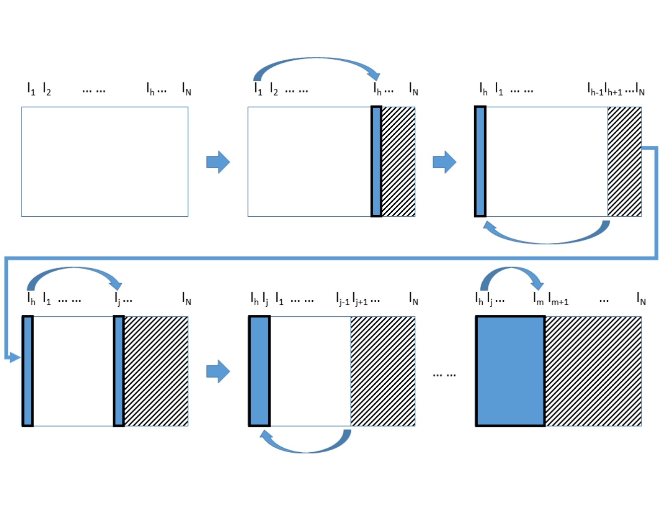
We first present FA algorithm for deriving one solution of minimal unique (Definition 4), with a size (number of columns) no bigger than . Given a sequence of column indices which is a permutation of , FA Algorithm attempts to find in at most sweeps of . We start with an empty set and in each sweep, one element of is added to until . The algorithm is presented both in pictorial (Figure 1) and pseudo code form (Algorithm 1). A detailed description is as follows.
Input: , a permutation of
First, initialize , and (line 1 and the first panel). Next, we create a temporary set of columns that is identical to (line 3). We now add indices in one by one to until for the first time the distinct row count for column combination reaches (line 4-6 and panel 2). Suppose this is the th element in . From here, we can conclude that must contain a solution set of minimal unique, and column is required in the solution, so we add to and ignore the remaining columns after the first columns in (line 7-8 and panel 3 in the figure where the shaded columns are to be discarded). This completes one sweep of . With an updated , we go back to Step 2 and repeat this process at most times where in each time we find one column in to add to solution set until either or we exceed the size limit (line 2 in algorithm, and 4th and 5th panels of Figure 1 shows the second iteration of this). If , then is a minimal unique with . Otherwise we failed to find a solution (line 9 or panel 6).
It is helpful to understand how FA algorithm works in the case of multiple minimal uniques using illustrative examples. Let the initial be . Assume first is the only minimal unique. Then FA algorithm would find column 6 first, then column 4, and finally column 1 to add to in three sweeps of (where each time shrinks by discarding the elements after the selected one (shaded columns in Figure 1)). Now suppose there are two solutions: and . As the largest numbers in and are 6 and 7 respectively, and 6 is less than 7, FA algorithm would return as the solution since the search reaches first (line 4 and 5). Suppose the two solutions are: . In this case the largest number in each solution set ties (both are 6). Then after 6 is added to , since from is less than from , this becomes the tiebreaker with the addition of the 2nd column index, which would return as the solution. In general, FA would return with a solution whose largest column index in the permuted table is the smallest among all solutions. If there is a tie, the tie-breaker would be determined by next additions in the same manner.
3.2. Computational Complexity
During each sweep, column indices in are incrementally added to a temporary set until the distinct row count reaches (line 5-6 of Algorithm 1). Since the distinct row count with respect to column addition is strictly increasing until it hits , if the number of columns is large, we can use binary search to locate this column with distinct count evaluations. Therefore, with sweeps, the total distinct count evaluations is . In comparison, the required distinct count evaluations for BE algorithm (Section 2) is for the case of , which implies FA is less expensive than BE for a table with a large number of columns .
Theorem 1.
One run of Forward Addition (FA) algorithm requires distinct count evaluations while one run of Backward Elimination (BE) algorithm requires distinct count evaluations.
3.3. FA algorithm with Random Column Permutation
In Algorithm 1 line 1, is a permutation of the original column indices . We analyze the probabilistic properties of FA algorithm where the index sequence is a random permutation of , especially when there are multiple competing minimal uniques. Suppose there exists at least one minimal uniques with size no bigger than . We also discuss the success probability that one run of the randomized FA algorithm will find a desired solution.
Suppose a column combination is a minimal unique with columns. Given a random permutation of , let be the index of each of in . For example, suppose is a minimal unique. With a random permutation of , their corresponding indices in becomes respectively. This means, the 5th column in is the 1st column in the original table, the 3rd column in is the 4th column in the original table and the 9th column in is the 6th column in the original table.Then . For with a large , it can be shown that can be approximated by independent and identically distributed (i.i.d.) uniform random variables on . Let , which is the largest index of the solution set after permutation, divided by . Then where are i.i.d. uniform. It is easy to show that has the following approximate distribution: . We summarize the result in the following lemma.
Lemma 0.
Suppose we are given a table and a column combination of indices, . After a random column permutation of table , let denote the new index of in the permuted table. Then as the total number of columns , approximates independent random variables. Furthermore, let . Then for any as .
Now suppose there are minimal uniques, with length . Let
| largest index of in the randomly column | ||||
As we show before, if there is no ties in , FA will return the solution whose is the smallest. For the special instance of two minimal uniques with length and no-overlapping elements, simple calculations by integration show that
| (1) |
Therefore, if , then , and the probability goes to 1 as becomes increasingly larger than . This implies that FA would probabilistically favor the shorter solutions. It is easy to extend the conclusion to the case when that share common elements by separating out the common elements from the non-overlapping elements and use similar integration calculations. We have the following lemma.
Lemma 0.
Let be two minimal uniques with length and respectively. If then
where is the maximal index value defined in Lemma 2. This implies that if and are the only two minimum uniques, FA algorithm with random column permutation would favor as the returned solution as the probability of returning is higher than that of .
The above lemma can be generalized to multiple solutions, and to the case with arbitrary solution lengths (not necessarily ). However, the extension to the most general case when the solutions sets are overlapping may need careful treatment.
Theorem 4.
FA with random column permutation (i.e., is a random permutation of tends to favor the shorter solutions of minimal unique. In particular, if are the solution sets with length that are non-overlapping, then the probability that be the final returned solution is the highest.
Suppose there exist solutions with a size no bigger than out of all minimal uniques. Let be the event that we successfully finds a minimum unique with size constraint after one run of FA with random permutation. Then by Theoroem 4, is at least . Therefore, for a finite and an arbitrary small , we can find the a max failure times parameter such that . If there are consecutive failures, we can probabilistically declare that there is no minimal uniques with size less or equal to . It is worthwhile to mention that the performance of BE algorithm is identical to FA in terms of success probabilities when the columns are randomly permuted.
3.4. Extension to Functional Dependency
We generalize Algorithm 1 to the case of functional dependence. The generalization also considers approximate functional dependence defined below. Again let be two column combinations in Table . We consider two definitions of error measurement in order to define approximate functional dependency: .
Definition 0.
Let be the minimal fraction of rows to be removed for to hold. Then , if .
Definition 0.
Define , then if
It is easy to show the following lemma that states a monotone property of the error measures with column additions.
Lemma 0.
iff . For a given , is non-decreasing with column additions to . is non-decreasing with column additions to when columns in the addition are chosen from .
We use two error definitions here due to computational considerations. Error in Definition 6 is much easier to compute than Definition 5 (which can be computed using algorithms in (Huhtala:1999)). Furthermore, as Lemma 1 indicates, both definitions coincide when the error is 0. Unfortunately, the error in Definition 6 lacks a monotone property in the general case with column additions, unless the columns are from . However, this special case is indeed what we use to build a schema tree in Section 5. In the following, Algorithm 2 extends FA algorithm to general functional dependence in a straightforward fashion, by replacing the check for minimal uniqueness with the check for functional dependency (line 2, 6 and 9). The key to this extension is the monotonic property of the errors in Lemma 7.
Input: , a sequence of column indices after column permutation
4. Best Solution with Size and Error Constraints
For a set of columns from a data table , in this section, we propose algorithms to find best solutions of such that with for a given error and size . These algorithms essentially run FA algorithm (Algorithm 2) multiple times where in each iteration we attempt to improve upon previous solution until failure occurs. We consider the following two scenarios.
4.1. Shortest Solution with Error Bound
For a given and error upper bound , Algorithm 3 find a solution with the fewest number of columns with at most consecutive failures such that . The algorithm works with an input maximum number of consecutive failures after which we can declare no better solutions can be found. A call to Algorithm 2 is performed in each iteration (line 4) to attempt to find a solution with the given error bound and the current achievable minimal size (initialized to be ). After the first solution is found, the algorithm tries to find a better solution with a smaller size (fewer columns) if successful (line 6 and 7). The algorithm terminates if the maximum number of attempts has been reached or the solution size reaches 1 (line 2).
Input: Maximum number of consecutive failures (e.g. 10)
4.2. Shortest Solution while Minimizing Error
A more difficult situation is to find the shortest solution such that and while minimizing for a given (i.e. minimizing first, then the solution size). A naive approach is to run Algorithm 3 on a grid of values, , and return the solution with the minimal possible . If multiple solutions exist with the minimal value of , return the shortest one.
Algorithm 4 provides an alternative for finding the minimal using hill climbing, avoiding the grid search with at most consecutive failures. In the first iteration, it finds a candidate solution by running Algorithm 2 (line 3-4). Next, it attempts to reduce the error rate using sequential column additions to with the max size , i.e., (line 5,6). This is due to the fact that, from Lemma 7, the error rate can be reduced with column additions. We assign this updated column set as our initial solution along with its error rate . In the following iterations, we perform a similar updating process (line 3, 4, 7-10) in the attempt to achieve an even smaller error rate until we fail consecutively times. At this point, we have found the smallest reachable . Finally, we find the shortest solution using Algorithm 3 with the given minimum value of (line 11, 12).
Input: Maximum number of consecutive failures (e.g. 10)
4.3. Discussion
In this section, we proposed algorithms to find the best solution of a column combination that functionally determines for given size and error constraints, using multiple iterations of FA algorithm with random column permutations. Our algorithms avoid the exhaustive search of all solutions and utilize the fact that FA algorithm favors a short solution (Theorem 2). We want to point out that if the goal is to find all solutions of that functionally determines , then running many iterations of FA algorithm with independent column permutations is not efficient. This is because the number of all permutation is for a table with columns, a number much larger than the number of all subsets, (the maximal number of solutions of ). That said, we believe more efficient algorithms can be developed for finding multiple solutions of by adaptively choosing column permutations based on previous found solutions. For example, if is a first solution found by one run of FA, then in the next iteration, we can place last in and randomly reorder the remaining columns. This way, we are guaranteed to find a different solution if it exists (since the indices of the 2nd solution will appear earlier). We leave this to future work.
| orderID | productID | customerID | time | ordertype | fullname | phoneno | age | ptype | price | weight | shippingcost |
|---|---|---|---|---|---|---|---|---|---|---|---|
| 1 | 1 | 4 | day 1 | web | Alex Smith | 732-906-9882 | 29 | book | 15 | 0.5 | 4.5 |
| 1 | 6 | 4 | day 1 | web | Alex Smith | 732-906-9882 | 29 | music | 11 | NA | NA |
| 2 | 3 | 2 | day 1 | web | Emma Miller | 908-654-3213 | 36 | beauty | 39 | 0.2 | 4.2 |
| 3 | 2 | 2 | day 2 | web | Emma Miller | 908-654-3213 | 36 | clothing | 32 | 0.6 | 4.6 |
| 3 | 4 | 2 | day 2 | web | Emma Miller | 908-654-3213 | 36 | games | 18 | NA | NA |
| 3 | 6 | 2 | day 2 | web | Emma Miller | 908-654-3213 | 36 | music | 11 | NA | NA |
| 4 | 5 | 3 | day 2 | phone | Kim Dole | 973-211-1245 | 45 | grocery | 25 | 1 | 2.3 |
| 4 | 5 | 3 | day 2 | phone | Kim Dole | 973-211-1245 | 45 | grocery | 12 | 1 | 2.3 |
5. Building a Schema Tree
In this section, we present an algorithm that builds a schema tree for a data table using recursive functional dependency discovery. The schema tree represents the structure dependency between table columns in a simple hierarchical form. As a result, it is possible to decompose a big data table into layers of smaller tables. In the next section, we show how this information is utilized for automated feature engineering.
Input: size parameter , error parameter
Output: Schema tree skeleton
Our schema tree is built via a two-step process. In the first step, we build the tree skeleton using Algorithm 5. Given a table , we first add a hypothetical rowid column as the row index and start building the tree using this as the root node (line 9). Let be the current node of interest. Then we attempt to split using columns from the set (Definition 3 and line 3). A split is found if there exists a solution such that and using Algorithm 3 or 4 (depending on the application context), for the given size constraint and error constraint (line 4). If a solution is found, then we split by nodes in as its children. Such a splitting process is done recursively for all nodes in (line 6,7) until we are no longer able to split (line 5). Note when , such a split indicates a bi-directional functional dependency (or equivalence) between and since is derived from . It is important to note that for well designed data tables, the skeleton nodes are usually not decimal valued numeric columns. Therefore we do not include these columns when building the tree skeleton.
Once the schema skeleton is built, the second step is to add the remaining columns to complete the tree construction. For each of the remaining nodes, we attach it to the deepest skeleton node that it functionally depends. As explained in Section 2, this can be done by a simple row distinct count check. In the following, we shall elaborate our process using simulated and real data.
5.1. Illustrative Examples
Table 1 displays sample rows of a simulated table that stores information related to customer purchase orders on an e-commerce website: an order is placed by a customer at a specific time, and each order can contain multiple products spanning multiple rows. The table also contains the associated customer and product information. Here proper column names are shown with the contextual information so that a domain expert can easily understand the structure relations between columns. Understanding column relations will be much more difficult if this contextual information is removed.
Figure 2 shows the discovered schema tree with and , where the red node is the root node representing the row index, blue nodes indicate the discovered tree skeleton using Algorithm 5, and the gray nodes are the rest of the leaf nodes attached in the second step of tree construction. Let indicate the joint bidirectional functional dependency, and as before, let indicate functional dependency. Figure 2 can be interpreted as follows:
where the first two rows are regarding to the blue nodes, and the next two are sample relations concerning the gray nodes. The tree skeleton (red and blue nodes) is built using Algorithm 5 while removing weight and shippingCost as these are decimal valued columns and not initially included (decimal valued numeric columns can be auto-detected by methods in (huseyin.sdd)). In the second step, we attach each of the remaining columns (gray nodes) to the deepest blue (or red) node that it functionally depends. With this schema tree, we can actually extract several smaller tables: a ’Product’ table from productID and its children, a ’Customer’ table from CusomterID and its children, and a smaller ’Order’ table from orderID and its children. Our big table is, in fact, the merge of these three tables.
The second dataset contains broadband home router data records of customers from a network carrier during a 30-day period. It consists of columns and rows, where columns are device’ ID, type, associated network nodes and types, the customer information, and time series of several KPIs.
Figure 3 shows the discovered schema tree with and . The first split from the red root node representing row index is , and the next split is . Furthermore, , , . The leftmost 6 gray nodes are associated KPI time series (it is time related by noticing the day.1 of the 1st split from the root), and the rightmost gray nodes are device-related attributes. Again, with the schema tree, we can decompose the table into layers of ’Device’ table from node deviceid, a ’customerattr2’ table from node customerattr2, and a KPI time series table for each customerattr2/ start_gp combination. Understanding the column relations is much more straightforward with our diagram.
Finally, we want to comment that the schema tree derived from our algorithm may not be unique, especially for tables with complex column relationship. For example, if there are multiple short functional dependencies with the same length, the algorithm will randomly pick one of these to follow through. Figure 4 shows two different realizations of our algorithm for an internal data table named ’Project’ describing the progress of ongoing projects. From the root node , both scheme trees find a single column as the 1st level descendant. However, the trees differ in the next blue node split: the tree on the left is split by , and the tree on the right is split by (). Although both solutions are valid, one may prefer the first scheme tree. This is because is the combination of a label and DateTime column, but are two DateTime columns, and the formal is a more natural table key than the latter. In this case, we are using the contextual information in the columns to select a more appropriate solution. How to automatically infer the contextual information of columns and utilize this in the selection of schema tree is part of our future work.
6. Applications to Auto Feature Engineering
Our schema tree built automatically from a data table not only provides valuable information for the data scientists to better understand the table, it can also directly benefit the downstream machine learning tasks. In this section, we show how information from the schema tree can be used for automated feature engineering. Traditionally, feature engineering often requires handcrafting based on contextual understanding.
We shall illustrate this using the simulated order Table 1. Suppose ’CustomerID’ is an anchor node ’customer’ and we are interested in engineering features for each customer. First, we notice that there are two types of relationship from CustomerID to any other node: one-to-one and one-to-many. In the one-to-one relation, each CustomerID determines a single instance of the other variable, which in fact implies that these variables are either functional equivalent to or descendants of CustomerID in the schema tree. The remaining nodes in the schema tree have a one-to-many relation from CustomerID which imply that each CustomerID corresponds to multiple instances of the variable.
In this example, CustomerID has three gray nodes as descendants: age , fullname, phoneno. This implies that for each of the three nodes, there is a one-to-one relation from CustomerID, so we can take the instance value directly as a feature for each CustomerID. On the other hand, for each of the remaining columns, there is a one-to-many relation as each distinct CustomerID will have one or several instances of its values. (Take the node Price as an example. In Table 1, Customer 4 have 2 price instances, Customer 2 have 4 price instances.) Therefore we need to aggregate these values to create a uniform number of features for each CustomerID. In this case, for any node , we first find the shortest path from CustomerID to in the schema tree, which gives us a bottom-to-top aggregation path towards CustomerID. For example, the path from Price to CustomerID while ommiting rowid as it is a hypothetical node is: We further omit the one-to-one relations in the path as no aggregation is necessary, and so the aggregation path is simplified to where indicates a many-to-one relation. Finally, we extract all the subpaths and use a set of pre-specified aggregation functions to generate features. Specifically, Price is aggregated by
|
|
where are pre-specified aggregation functions depending on the characteristics of the variable to be aggregated. For numeric variables, these functions can be max, mean, standard deviation, interval probabilities or quantiles. For categorical variables, it can be distinct counts. This way we can come up with a set of features such as: the maximum () of average () price per orderID, or the standard deviation () of the price. This approach is related to recent research on automated feature engineering (DFS-MIT; OneBM). However, these methods focuses on relational databases with a known schema with an assumption that each table has a shallow structure. In contrast, our method proposed here do not assume prior schema knowledge and can work with data tables with layered structure. In addition, our methods can also be extended relational databases by joining schema graphs together (not illustrated here).
7. Conclusion
In this paper, we developed an automatically-generated, data-driven schema tree to represent the structural relations between columns of a data table that can greatly facilitate a data scientist when exploring a new dataset. The key to our approach is the recursive extraction of important functional dependency between columns of the data table, where we proposed a forward addition algorithm that requires much less computation compared to existing approaches.
References
- (1) M. Feurer, A. Klein, K. Eggensperger, J. Springenberg, M. Blum, and F. Hutter, “Efficient and robust automated machine learning,” Proceedings of the 28th International Conference on Neural Information Processing Systems, pp. 2755–2763, 2015.
- (2) K. Pearson, “Note on regression and inheritance in the case of two parents,” Proceedings of the Royal Society of London, vol. 58, pp. 240–242, 1895.
- (3) C. E. Shannon, “A mathematical theory of communication.” Bell Syst. Tech. J., vol. 27, no. 3, pp. 379–423, 1948. [Online]. Available: http://dblp.uni-trier.de/db/journals/bstj/bstj27.html#Shannon48
- (4) D. Koller and N. Friedman, Probabilistic Graphical Models: Principles and Techniques, ser. Adaptive computation and machine learning. MIT Press, 2009. [Online]. Available: https://books.google.co.in/books?id=7dzpHCHzNQ4C
- (5) Y. Huhtala, J. Kaerkkaeinen, P. Porkka, and H. Toivonen, “Tane: an efficient algorithm for discovering functional and approximate dependencies.” The Computer Journal, p. 42(2):100–111, 1999.
- (6) A. Heise, J.-A. Quiané-Ruiz, Z. Abedjan, A. Jentzsch, and F. Naumann, “Scalable discovery of unique column combinations,” Proc. VLDB Endow., vol. 7, no. 4, pp. 301–312, Dec. 2013. [Online]. Available: http://dx.doi.org/10.14778/2732240.2732248
- (7) S. Lopes, J.-M. Petit, and L. Lakhal, “Efficient discovery of functional dependencies and armstrong relations,” in International Conference on Extending Database Technology. Springer, 2000, pp. 350–364.
- (8) C. Wyss, C. Giannella, and E. Robertson, “Fastfds: A heuristic-driven, depth-first algorithm for mining functional dependencies from relation instances extended abstract,” in International Conference on Data Warehousing and Knowledge Discovery. Springer, 2001, pp. 101–110.
- (9) Y. Sismanis, P. J. H. P. Brown, and B. Reinwald, “Gordian: Efficient and scalable discovery of composite keys.” In VLDB, pp. 691–702, 2006.
- (10) Z. Abedjan and F. Naumann, “Advancing the discovery of unique column combinations.” International Conference on Information and Knowledge Management (CIKM), p. 1565–1570, 2011.
- (11) T. Papenbrock and F. Naumann, “A hybrid approach for efficient unique column combination discovery,” in Datenbanksysteme für Business, Technologie und Web (BTW 2017), B. Mitschang, D. Nicklas, F. Leymann, H. Schöning, M. Herschel, J. Teubner, T. Härder, O. Kopp, and M. Wieland, Eds. Gesellschaft für Informatik, Bonn, 2017, pp. 195–204.
- (12) H. Uzunalioglu, J. Cao, C. Phadke, G. Lehmann, A. Akyamac, R. He, J. Lee, and M. Able, “Augmented data sciencetowards industrialization and democratization of data science,” Nokia Bell Labs, Tech. Rep., 2019.
- (13) J. M. Kanter and K. Veeramachaneni, “Deep feature synthesis: Towards automating data science endeavors,” in Data Science and Advanced Analytics (DSAA), 2015. 36678 2015. IEEE International Conference on. IEEE, 2015, pp. 1–10.
- (14) H. T. Lam, J.-M. Thiebaut, M. Sinn, B. Chen, T. Mai, and O. Alkan, “One button machine for automating feature engineering in relational databases,” arXiv preprint arXiv:1706.00327, 2017.