.
Heat fluctuations in equilibrium
Abstract
The characteristic function for heat fluctuations in a non equilibrium system is characterised by a large deviation function whose symmetry gives rise to a fluctuation theorem. In equilibrium the large deviation function vanishes and the heat fluctuations are bounded. Here we consider the characteristic function for heat fluctuations in equilibrium, constituting a sub-leading correction to the large deviation behaviour. Modelling the system by an oscillator coupled to an explicit multi-oscillator heat reservoir we evaluate the characteristic function.
pacs
05.40.-a, 05.70.LnI Introduction
There is a current interest in the thermodynamics and statistical mechanics of small fluctuating systems in contact with heat reservoirs and driven by external forces. This interest stems from the recent possibility of the direct manipulation of nano systems and biomolecules in non equilibrium scenarios Trepagnier et al. 2004; Collin et al. 2005; Tietz et al. 2006; Blickle et al. 2006; Imparato et al. 2007; Douarche et al. 2006; Garnier and Ciliberto 2007; Imparato et al. 2008. together with the advent of the so-called fluctuation theorems which impose symmetry relations on the non equilibrium heat and work probability distributions Jarzynski 1997; Kurchan 1998; Gallavotti 1996; Crooks 1999; Crooks 2000; Seifert 2005a; Seifert 2005b; Evans et al. 1993; Evans and Searles 1994; Gallavotti and Cohen 1995; Lebowitz and Spohn 1999; Gaspard 2004; Imparato and Peliti 2006; van Zon and Cohen 2003a; van Zon et al. 2004; van Zon and Cohen 2003b; van Zon and Cohen 2004; Speck and Seifert 2005. In recent years there has also been increased interest in the above non equilibrium issues for open quantum systems, see e.g. Salazar et al. 20019; Denzler and Lutz 2018.
As an illustrative example we consider a single oscillator coupled to two heat reservoirs at temperatures and and characterised by the damping constants and , respectively Derrida and Brunet 2005; Fogedby and Imparato 2011. The representative Langevin equations for the position , the momentum , force constant , heat flux from reservoir 1, and noises and are then given by (setting the mass )
| (1) | |||
| (2) | |||
| (3) | |||
| (4) | |||
| (5) |
The characteristic function describing the long time behaviour of the heat fluctuations is given by
| (6) |
where is the large deviation function. The general Gallavotti-Cohen fluctuation theorem applying to nonequilibrium systems implies the fundamental symmetry Gallavotti and Cohen 1995; Fogedby and Imparato 2011
| (7) |
For the above example we have explicitly Derrida and Brunet 2005; Fogedby and Imparato 2011
| (8) | |||
| (9) |
where the form of implies the fluctuation theorem. Disconnecting for example reservoir 1 by setting the large deviation function vanishes. The resulting system with an oscillator interacting with a single reservoir is an equilibrium system with bounded heat fluctuations and .
The purpose of the present paper is to investigate further the case of fluctuations in equilibrium described by the characteristic function . In the case of a thermodynamic variable the understanding is well known and follows from the Boltzmann-Gibbs scheme Landau and Lifshitz 1980; Reichl 1998. The probability distribution is determined by the entropy according to Landau and Lifshitz 1980; Reichl 1998. Expanding about the its maximum value corresponding to equilibrium, i.e., , we arrive at the Gaussian distribution , where is the mean square fluctuation.
However, in the case of the fluctuating heat exchanged between a small system and a single heat reservoir at inverse temperature (we have set the Boltzmann constant ), the heat distribution , surprisingly, does not take a Gaussian form. As discussed in previous papers Imparato et al. 2007; Fogedby and Imparato 2009 addressing an over damped oscillator, the distribution has the form , where is a Bessel function Lebedev 1972; Gradshteyn and Ryzhik 1965. This distribution only depends on the temperature of the reservoir, exhibits exponential Boltzmann tails and diverges logarithmically at small as .
In general the characteristic function, defined according to Reichl 1998
| (10) |
is given by the expression
| (11) |
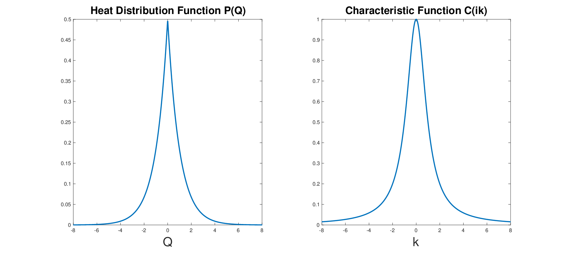
where is the partition function for the system Landau and Lifshitz 1980; Reichl 1998. We note that in the case of a single over damped oscillator with one degree of freedom , i.e., . Likewise, for a damped harmonic oscillator with two degrees of freedom coupled to a reservoir , yielding the characteristic function . The corresponding heat distribution is , decaying exponentially and exhibiting a cusp at .
We note that in the presence of two temperature-biased heat reservoirs driving the system into a non equilibrium state, a finite fluctuating heat flux will be established. As a result the integrated heat will on average grow linearly in time, i.e., . More precisely, the characteristic function associated with the probability distribution , , where is the large deviation function; in equilibrium we have . In that sense the equilibrium heat distribution constitutes the sub-leading correction to the large deviation result.
In the present paper we extend the analysis in Fogedby and Imparato 2009 and consider the case of an explicitly defined heat reservoir in evaluating the equilibrium heat distribution. For convenience we consider the case of a single oscillator coupled to single heat bath. The explicit characterisation of the heat bath in terms of a collection of oscillators is well known and a prerequisite for a quantum treatment. It is also well known that the so-called ohmic approximation is equivalent to a standard Langevin/Fokker Planck description. However, we believe that the present calculation carried out within the multi-oscillator scheme is novel.
The paper is organised in the following manner. In Sec. II we define the heat exchanged between the system and the reservoir. In Sec. III we discuss a heuristic derivation of the characteristic function, yielding Eq. (11). In Sec. IV we discuss the explicit characterisation of the heat bath in terms of a collection of oscillators. In Sec. V we turn to an evaluation of the heat characteristic function in the case of a multi-oscillator heat bath. Since the methods we employ are well known we defer technical details to appendix A and B sections.
II Heat
A small system coupled to a heat reservoir constitutes a closed system. Correspondingly, the total energy of system and reservoir is conserved. However, the small system itself exchanges energy with the reservoir and is in this respect and open system.
Let us characterise the small fluctuating system coupled to the heat reservoir by the fluctuating Hamiltonian , where are the degrees of freedom. The time dependence of is due to the heat reservoir and not to an applied external time dependent force, i.e, we are not applying an external protocol as is common in the context of fluctuation theorems Jarzynski 1997; Kurchan 1998; Gallavotti 1996; Crooks 1999; Crooks 2000; Seifert 2005a; Seifert 2005b; Evans et al. 1993; Evans and Searles 1994; Gallavotti and Cohen 1995; Lebowitz and Spohn 1999; Gaspard 2004; Imparato and Peliti 2006; van Zon and Cohen 2003a; van Zon et al. 2004; van Zon and Cohen 2003b; van Zon and Cohen 2004; Speck and Seifert 2005.
The fluctuating heat flux from the reservoir to the small system is thus given by . Note that since we are in equilibrium the mean value . Consequently, the heat transmitted in a time span is , i.e.,
| (12) |
The transmitted heat is a fluctuating quantity and the issue is to determine its stationary probability distribution , or, equivalently, its characteristic function
| (13) |
III Heat distribution - heuristic derivation
Here we present a heuristic derivation of the heat distribution or characteristic function; this approach was also discussed in Fogedby and Imparato 2009 and is based on the definition in Eq. (12). From Eqs. (12) and (13) we have
| (14) |
Assuming that the system is in equilibrium at time and at time and, moreover, assuming that is larger than the characteristic decay time of fluctuations, the energy fluctuations at time and time can be assumed to be uncorrelated and we infer . An interesting side issue is the role of finite time correlations; this will, however, not be considered here. Finally, averaging with respect to the canonical ensemble, , for a heat reservoir maintained at temperature , we arrive at Eq. (11), i.e.,
| (15) |
In the case of two degrees of freedom, e.g., for a harmonic oscillator coupled to a heat bath, where Landau and Lifshitz 1980; Reichl 1998, we obtain
| (16) |
IV Multi-oscillator heat bath
Here we derive the characteristic function introducing an explicit representation of the heat reservoir in terms of a system of non-interacting oscillators. In a quantum context this is a standard approach Ford et al. 1965; Ford and Kac 1987; Ford et al. 1988; Caldeira and Leggett 1983; Caldeira 1983 and we therefore defer technical details to Appendix VII.1. The total system consisting of the oscillator coupled to the heat bath is isolated and globally energy conserving. The oscillator itself can exchange energy with the reservoir and is in this regard an open system. The total system is described by the oscillator Hamiltonian , a Hamiltonian for the heat bath together with an interaction term to be specified later. We have
| (17) | |||
| (18) |
where is the mass and the frequency of the oscillator. The bath oscillators have mass and frequencies , where is the wave number.
The analysis is simplified by introducing the complex amplitude variables and , see Appendix VII.1, yielding the Hamiltonians
| (19) | |||
| (20) |
For the interaction between the oscillator and the heat bath we choose the linear coupling
| (21) |
where the coupling strength is assumed weak. By appropriate choice of the phases of and we can ensure that is real. We note that the interaction Hamiltonian differs from the shift interaction used by Ford Ford et al. 1965; Ford and Kac 1987; Ford et al. 1988. In the present case the interaction corresponds to the rotating wave approximation employed in quantum optics Gardiner 1997; Fogedby 1993; Glauber and Man’ko 1984.
In the ohmic approximation Ford et al. 1965; Ford and Kac 1987; Ford et al. 1988; Caldeira and Leggett 1983; Caldeira 1983 and at long times the amplitude of the oscillator is given by
| (22) |
where the renormalised frequency , the shift and the damping are given by
| (23) | |||
| (24) |
Here is the initial value of the amplitude of the k-th reservoir mode. In the limit of a large reservoir time smoothing is implemented and we have , where is incorporated in the definition of the density of states . For and we then obtain
| (25) | |||
| (26) |
It is instructive to show that the oscillator locks onto the reservoir temperature at long times. Inserting the solution in Eq. (22) in Eq. (19) and using equipartition of the k-the mode, i.e., , we obtain for the mean value of
| (27) |
demonstrating equipartition for the oscillator due to coupling to the heat reservoir
V Heat distribution
Regarding the characteristic function for the heat we obtain, inserting from Eq. (12) and averaging over the initial reservoir states according to , the functional integral
| (28) |
where we have used . Inserting the solution in Eq. (22) in in Eq. (19) the functional integral (28) has a Gaussian form and can be performed using standard techniques Zinn-Justin 1989. By mean of the identity the evaluation of (28) is reduced to an eigenvalue problem. Deferring details to Appendix VII.2 we obtain the characteristic function in Eq. (16), i.e., .
VI Discussion
In this paper we have discussed heat fluctuations in equilibrium for an oscillator driven by a single heat reservoir. A simple heuristic argument yields the characteristic function only depending on the inverse temperature . However, the main purpose of the present work is to demonstrate that this result is also obtained by an explicit representation of the heat reservoir as a collection of independent oscillators; a representation of a heat bath often used in a quantum mechanical context. We believe this approach is novel in the context of heat fluctuations. We have discussed the problem in terms of complex amplitude variables, the classical counterpart of creation and annihilation operators for quantum oscillators. The linear coupling to the reservoir is implemented within the rotating wave approximation, used in quantum optics. We, moreover, notice that the ohmic approximation, yielding the usual Langevin description with damping and white noise, here is equivalent to the quasi particle approximation, known from quantum many body theory. In Fig. 1 we have depicted the characteristic function and the associated heat distribution.
VII Appendices
VII.1 Multi-oscillator heat bath
The oscillator and the heat bath are described by the Hamiltonian in Eq. (17) and in Eq. (18), where the coordinates and momenta satisfy the Poisson brackets Landau and Lifshitz 1959
| (29) | |||
| (30) |
Introducing the complex amplitude variables Breuer and Petruccione 2002
| (31) | |||
| (32) |
we have the Poisson brackets
| (33) | |||
| (34) |
and the Hamiltonians , , and in Eqs. (19), (20), and (21). Noting that the total Hamiltonian is time independent we obtain from the general equation of motion :
| (35) | |||
| (36) |
Introducing the Laplace transform Lebedev 1972; Mathews and Walker 1973
| (37) | |||
| (38) |
with just above the real axis, i.e., , the equations of motion take the form
| (39) | |||
| (40) |
where and denote the initial values. Solving for and we find
| (41) | |||
| (42) |
where we have introduced the self energies
| (43) | |||
| (44) |
Using the Plemelj formula we obtain for
| (45) | |||
| (46) | |||
| (47) |
In the weak coupling limit we can make the quasi particle approximation well known in many body theory Mahan 1990 and replace by , i.e.,
| (48) | |||
| (49) |
In the present context the weak coupling quasi particle approximation corresponds to the ohmic approximation Ford et al. 1965; Ford and Kac 1987; Ford et al. 1988. Absorbing the shift in a renormalisation of , i.e., defining , we obtain for the oscillator amplitude
| (50) |
and in time
| (51) |
For we have ; at long times for we obtain Eq. (22), i.e.,
| (52) |
Regarding the reservoir modes we obtain solving Eq. (42) for
| (53) |
In time we have
| (54) | |||||
For we have ; at long times for we obtain
| (55) | |||||
In the limit of a large heat reservoir the discrete spectrum of reservoir modes labeled by the wavenumber becomes a continuum. Replacing by the integral , where the density of states incorporates the coupling , we obtain
| (56) | |||
| (57) | |||
| (58) |
The continuum limit thus automatically implies irreversibility and the separation of time scales. These two assumptions are encoded in the standard classical Langevin/Fokker Planck approach. The long time expressions for the fields and in Eqs. (52) and (55) are easy to interpret. Regarding we notice that the dependence on the initial value drops out and is entirely driven by the heat reservoir thus depending on the initial heat reservoir characterised by ; the heat reservoir gives rise to damping and at the same time locks onto . Regarding the reservoir amplitudes there is a first order ”back action” on the k-th mode from the oscillator and an induced second order interaction between the modes.
VII.2 Multi-oscillator heat bath derivation of
In order to evaluate the distribution we must keep track of the energy flow or heat between the reservoir and the oscillator. In the weak coupling limit we can ignore the energy stored in the interaction term given by (21) and identify the heat with the increase of the oscillator energy in the time span . Consequently, is given by Eq. (12), i.e. , where . Inserting the solution in Eq. (52) we arrive at
| (59) | |||
| (60) | |||
| (61) |
For the characteristic function in Eq. (14) we then obtain
| (62) |
where we average over the bath amplitudes at time . Using the identity
| (63) |
and inserting from Eq. (20) we have
| (64) |
In order to evaluate the determinant we consider the eigenvalue problem
| (65) |
Inserting from Eqs. (60) and (61) we have
| (66) | |||
| (67) | |||
| (68) |
Solving Eq. (66) for and inserting in Eqs. (67) and (68) we obtain the linear system
| (69) | |||
| (70) |
implying the determinantal condition
| (71) |
Further reduction inserting yields the condition
| (72) |
determining the eigenvalues . In the continuum limit inserting the density of states we have
| (73) |
Integrating over and to leading order in setting and introducing we obtain
| (74) |
or the eigenvalues
| (75) |
yielding
| (76) |
in agreement with in Eq. (16).
References
- Trepagnier et al. (2004) E. Trepagnier, C. Jarzynski, F. Ritort, G. Crooks, C. Bustamante, and J. Liphardt, Proc. Natl. Acad. Sci. USA 101, 15038 (2004).
- Collin et al. (2005) D. Collin, F. Ritort, C. Jarzynski, S. B. Smith, I. T. Jr, and C. Bustamante, Nature 437, 231 (2005).
- Tietz et al. (2006) C. Tietz, S. Schuler, T. Speck, U. Seifert, and J. Wrachtrup, Phys. Rev. Lett. 97, 050602 (2006).
- Blickle et al. (2006) V. Blickle, T. Speck, L. Helden, U.Seifert, and C. Bechinger, Phys. Rev. Lett. 96, 070603 (2006).
- Imparato et al. (2007) A. Imparato, L. Peliti, G. Pesce, G. Rusciano, and A. Sasso, Phys. Rev. E 76, 050101R (2007).
- Douarche et al. (2006) F. Douarche, S. Joubaud, N. B. Garnier, A. Petrosyan, and S. Ciliberto, Phys. Rev. Lett. 97, 140603 (2006).
- Garnier and Ciliberto (2007) N. Garnier and S. Ciliberto, Phys. Rev. E 71, 060101(R) (2007).
- Imparato et al. (2008) A. Imparato, P. Jop, A. Petrosyan, and S. Ciliberto, J. Stat. Mech p. P10017 (2008).
- Jarzynski (1997) C. Jarzynski, Phys. Rev. Lett. 78, 2690 (1997).
- Kurchan (1998) J. Kurchan, J. Phys. A 31, 3719 (1998).
- Gallavotti (1996) G. Gallavotti, Phys. Rev. Lett. 77, 4334 (1996).
- Crooks (1999) G. E. Crooks, Phys. Rev. E 60, 2721 (1999).
- Crooks (2000) G. E. Crooks, Phys. Rev. E 61, 2361 (2000).
- Seifert (2005a) U. Seifert, Phys. Rev. Lett. 95, 040602 (2005a).
- Seifert (2005b) U. Seifert, Europhys. Lett 70, 36 (2005b).
- Evans et al. (1993) D. J. Evans, E. G. D. Cohen, and G. P. Morriss, Phys. Rev. Lett. 71, 2401 (1993).
- Evans and Searles (1994) D. J. Evans and D. J. Searles, Phys. Rev. E 50, 1645 (1994).
- Gallavotti and Cohen (1995) G. Gallavotti and E. G. D. Cohen, Phys. Rev. Lett. 74, 2694 (1995).
- Lebowitz and Spohn (1999) J. L. Lebowitz and H. Spohn, J. Stat. Phys. 95, 333 (1999).
- Gaspard (2004) P. Gaspard, J. Stat. Phys. 117, 599 (2004).
- Imparato and Peliti (2006) A. Imparato and L. Peliti, Phys. Rev. E 74, 026106 (2006).
- van Zon and Cohen (2003a) R. van Zon and E. G. D. Cohen, Phys. Rev. Lett. 91, 110601 (2003a).
- van Zon et al. (2004) R. van Zon, S. Ciliberto, and E. G. D. Cohen, Phys. Rev. Lett. 92, 130601 (2004).
- van Zon and Cohen (2003b) R. van Zon and E. G. D. Cohen, Phys. Rev. E 67, 046102 (2003b).
- van Zon and Cohen (2004) R. van Zon and E. G. D. Cohen, Phys. Rev. E 69, 056121 (2004).
- Speck and Seifert (2005) T. Speck and U. Seifert, Eur. Phys. J. B 43, 521 (2005).
- Salazar et al. (20019) D. Salazar, A. Macedo, and G. Vasconcelos, Phys. Rev. E 99, 022133 (20019).
- Denzler and Lutz (2018) T. Denzler and E. Lutz, Phys. Rev. E 98, 052106 (2018).
- Landau and Lifshitz (1980) L. Landau and E. Lifshitz, Statistical Physics, Part 1 (Pergamon Press, Oxford, 1980).
- Derrida and Brunet (2005) B. Derrida and E. Brunet, Einstein aujourd’hui (EDP Sciences, Les Ulis, 2005).
- Fogedby and Imparato (2011) H. C. Fogedby and A. Imparato, J. Stat. Mech. p. P05015 (2011).
- Reichl (1998) L. E. Reichl, A Modern Course in Statistical Physics (Wiley, New York, 1998).
- Fogedby and Imparato (2009) H. C. Fogedby and A. Imparato, J. Phys. A 42, 475004 (2009).
- Lebedev (1972) N. N. Lebedev, Special functions and their applications (Dover Publications, New York, 1972).
- Gradshteyn and Ryzhik (1965) I. S. Gradshteyn and I. M. Ryzhik, Table of Integrals. Series, and Products (Academic Press, New York, 1965).
- Ford et al. (1965) G. W. Ford, M. Kac, and P. Mazur, J. Math. Phys. 6, 504 (1965).
- Ford and Kac (1987) G. Ford and M. Kac, Journal of Statistical Physics 46, 803 (1987).
- Ford et al. (1988) G. W. Ford, J. T. Lewis, and R. F. O’Connell, Phys. Rev. A 37, 4419 (1988).
- Glauber and Man’ko (1984) R. Glauber and V. I. Man’ko, JETP 60, 450 (1984).
- Caldeira and Leggett (1983) A. O. Caldeira and A. J. Leggett, Annals of Physics 149, 374 (1983).
- Caldeira (1983) A. O. Caldeira, Physica 121A, 587 (1983).
- Gardiner (1997) C. W. Gardiner, Handbook of Stochastic Methods (Springer-Verlag, New York, 1997).
- Fogedby (1993) H. C. Fogedby, Phys. Rev. A 47, 4364 (1993).
- Zinn-Justin (1989) J. Zinn-Justin, Quantum Field Theory and Critical Phenomena (Oxford University Press, Oxford, 1989).
- Landau and Lifshitz (1959) L. Landau and E. Lifshitz, Mechanics (Pergamon Press, Oxford, 1959).
- Breuer and Petruccione (2002) H. P. Breuer and F. Petruccione, The Theory of Open Quantum Systems (Oxford University Press, 2002).
- Mathews and Walker (1973) J. Mathews and R. L. Walker, Mathematical Methods of Physics (Benjamin Press, Menlo Park, 1973).
- Mahan (1990) G. D. Mahan, Many Particle Physics (Plenum Press, New York, 1990).