ALOHA Receivers: a Network Calculus Approach for Analyzing Coded Multiple Access with SICThanks: T.-H. Liu, C.-H. Yu, Y.-J. Lin, C.-S. Chang, and D.-S. Lee are with the Institute of Communications Engineering, National Tsing Hua University, Hsinchu 30013, Taiwan, R.O.C. Email: carina000314@gmail.com; chehaoyu@gapp.nthu.edu.tw; s107064901@m107.nthu.edu.tw; cschang@ee.nthu.edu.tw; lds@cs.nthu.edu.tw. This work was supported in part by the Ministry of Science and Technology, Taiwan, under Grant 109-2221-E-007-091-MY2, and in part by Qualcomm Technologies under Grant SOW NAT-435533.
Abstract
Motivated by the need to hide the complexity of the physical layer from performance analysis in a layer 2 protocol, a class of abstract receivers, called Poisson receivers, was recently proposed in [1] as a probabilistic framework for providing differentiated services in uplink transmissions in 5G networks. In this paper, we further propose a deterministic framework of ALOHA receivers that can be incorporated into the probabilistic framework of Poisson receivers for analyzing coded multiple access with successive interference cancellation. An ALOHA receiver is characterized by a success function of the number of packets that can be successfully received. Inspired by the theory of network calculus, we derive various algebraic properties for several operations on success functions and use them to prove various closure properties of ALOHA receivers, including (i) ALOHA receivers in tandem, (ii) cooperative ALOHA receivers, (iii) ALOHA receivers with traffic multiplexing, and (iv) ALOHA receivers with packet coding. By conducting extensive simulations, we show that our theoretical results match extremely well with the simulation results.
Keywords: multiple access, network calculus, successive interference cancellation, ultra-reliable low-latency communications.
I Introduction
The fifth-generation networks (5G) and beyond aim to cover three generic connectivity types: (i) enhanced mobile broadband (eMBB), (ii) ultra-reliable low-latency communications (URLLC), and (iii) massive machine-type communications (mMTC) (see, e.g., [2, 3, 4] and references therein). The reliability defined in 3GPP for supporting URLLC services, such as autonomous driving, drones, and augmented/virtual reality, requires the success probability of transmitting a layer 2 protocol data unit of 32 bytes within 1ms. On the other hand, the number of devices is in general much larger than the number of orthogonal resources for mMTC. Motivated by these emerging needs in 5G, many multiple access schemes have been proposed in the literature, see, e.g., Contention Resolution Diversity Slotted ALOHA (CRDSA) [5], Irregular Repetition Slotted ALOHA (IRSA) [6], coded slotted ALOHA (CSA) [7, 8, 9, 10], Low-Density Signature (LDS) based spreading [11], Sparse Code Multiple Access (SCMA) [12], Multi-User Sharing Access (MUSA) [13], Pattern Division Multiple Access (PDMA) [14], -fold ALOHA [15], Asynchronous Multichannel Transmission Schedules (AMTS) [16], Grant-free Hybrid Automatic Repeat reQuest (GF-HARQ) [17], and Polar Code Based TIN-SIC [18]. Though many of the above multiple access schemes use elegant message passing algorithms (or density evolution methods) for decoding as in the low-density parity-check codes [19], the decoding results depend heavily on the performance of the underlining physical channel. As such, it is very difficult to carry out further analysis in a layer 2 protocol, where there are multiple classes of input traffic and interconnected base stations/receivers/relays/antennas.
To hide the complexity from the physical layer, one needs an abstract model at the Medium Access Control (MAC) layer. Motivated by this, we proposed in our previous work [1] an abstract receiver, called Poisson receiver, that models the input-output relations of multiple classes of input traffic subject to an (independent) Poisson offered load. It was shown in [1] that various CSA systems in [6, 7, 8, 9, 10] can be modelled by Poisson receivers. In this paper, we take one step further to show that the block fading channel with capture in [20, 21, 10] can also be modelled by Poisson receivers. Poisson receivers have two elegant closure properties: (i) Poisson receivers with packet routing are still Poisson receivers, and (ii) Poisson receivers with packet coding are still Poisson receivers. Thus, one can use smaller Poisson receivers as building blocks for analyzing a larger Poisson receiver. Intuitively, Poisson receivers can be viewed as a probabilistic framework for analyzing coded random access.
In this paper, we propose a new class of abstract receivers, called ALOHA receivers, that can be viewed as a deterministic framework for analyzing coded multiple access with successive interference cancellation (SIC). Our approach is inspired by the theory of network calculus (see, e.g., the seminal works by Rene Cruz [22, 23], the books and the survey papers [24, 25, 26, 27, 28] and references therein). The theory of network calculus is a queueing theory that analyzes the network performance by viewing each queue as a building block with a certain arrival-departure property. By exploiting various elegant algebraic properties of the min-plus algebra [29], end-to-end delay bounds can be derived for various scheduling policies, including Generalized Processor Sharing (GPS) [30] and Service Curve Earliest Deadline first scheduling (SCED) [31].
Like a Poisson receiver, an ALOHA receiver is also an abstract receiver that views the underlining physical layer as a network element with a deterministic input-output function. Specifically, when there are class packets, , arriving at a -ALOHA receiver, the number of class packets that are successfully received (or successfully decoded) is exactly , . The function is called the success function of the -ALOHA receiver when it is subject to a deterministic load . On the other hand, the failure function, denoted by with represents the number of packets remained to be decoded.
One nice feature of coded multiple access with SIC is that a user can send multiple copies of a packet to a receiver. As long as one of the copies is successfully received, then the packet is successfully received, and the other copies of that packet can be removed from the receiver. Such a feature is known as the perfect SIC assumption in the literature (see, e.g., [10, 18]). As such, one can repeatedly apply the SIC operation to a receiver until there are no more packets that can be successfully decoded. Such an operation is even more interesting and powerful when a set of cooperative receivers can exchange information of successfully received packets.
The SIC operation induces several operations on functions, including minimum, composition, closure, and complement. Like the theory of network calculus, we develop various algebraic properties for these operations that can be used for proving various closure properties of ALOHA receivers, including
- (i)
-
two ALOHA receivers in tandem is also an ALOHA receiver in Section III-C,
- (ii)
-
two cooperative receivers is an ALOHA receiver in Section III-D,
- (iii)
-
ALOHA receivers with traffic multiplexing is an ALOHA receiver in Section III-E,
- (iv)
-
ALOHA receivers with packet coding is an ALOHA receiver in Section III-F, and
- (v)
-
multiple cooperative -fold ALOHA receivers is an ALOHA receiver in Section III-G.
An ALOHA receiver can be easily converted into a Poisson receiver. However, it is not the other way around. As such, the deterministic framework of ALOHA receivers can be incorporated into the probabilistic framework of Poisson receivers. To illustrate this, we provide a numerical example that uses two cooperative -fold ALOHA receivers with packet coding to provide differentiated services between URLLC traffic and eMBB traffic. For , such a system is reduced to the CSA system with two cooperative receivers in [1]. The theoretical results in this example match extremely well with the simulation results (except for those data points with extremely small error probabilities). Moreover, there is a significant performance gain by using the -fold ALOHA receivers over the -fold ALOHA receivers.
To provide a general overview of the probabilistic framework of Poisson receivers and the deterministic framework of ALOHA receivers, we depict in Figure 1 the basic building blocks and the associated calculus for analyzing coded multiple access with SIC.

The rest of the paper is organized as follows. In Section II, we briefly review the framework of Poisson receivers in our previous work [1]. There we also show how to model the Rayleigh block fading channel with capture as a Poisson receiver. We develop the deterministic framework of ALOHA receivers in Section III by proving various algebraic properties for several operations on functions. Using these algebraic properties, we then prove various closure properties of ALOHA receivers. In Section IV, we provide numerical examples to show how ALOHA receivers and Poisson receivers can be used for providing differentiated services between URLLC traffic and eMBB traffic. The paper is then concluded in Section V.
II Poisson receivers
II-A Review of the framework of Poisson receivers
In this section, we briefly review the framework of Poisson receivers in our previous work [1]. We say a system with classes of input traffic is subject to a Poisson offered load if these classes of input traffic are independent, and the number of class packets arriving at the system follows a Poisson distribution with mean , for .
Definition 1
(Poisson receiver with multiple classes of input traffic [1]) An abstract receiver is called a -Poisson receiver with classes of input traffic if the receiver is subject to a Poisson offered load , a tagged (randomly selected) class packet is successfully received with probability , for .
The throughput of class packets (defined as the expected number of class packets that are successfully received) for a -Poisson receiver subject to a Poisson offered load is thus
| (1) |
.
It was shown in [1] that many systems can be modelled by Poisson receivers, including SA, SA with multiple non-cooperative receivers, and SA with multiple cooperative receivers. Moreover, there are two elegant closure properties of Poisson receivers in [1].
- (i)
-
Poisson receivers with packet routing are still Poisson receivers.
- (ii)
-
Poisson receivers with packet coding are still Poisson receivers.
These two closure properties allow us to use smaller Poisson receivers as building blocks for analyzing a larger Poisson receiver.
Theorem 2
(Poisson receivers with packet routing [1]) Consider a Poisson receiver with classes of input traffic and the success probability functions . There are classes of external input traffic to the Poisson receiver. With the routing probability , a class external packet transmitted to the Poisson receiver becomes a class packet at the Poisson receiver. Let and with
| (2) |
. Then the system is a -Poisson receiver,
| (3) |
.
Using packet coding to increase system throughput has been widely addressed in the literature, see, e.g., [5, 6, 8, 7, 32, 33, 10]. The basic idea is to send a packet multiple times. If any one of them is successfully received, then the other copies of that packet can be removed from the system. Such an assumption is known as the perfect Successive Interference Cancellation (SIC) assumption. The decoding process is known as a peeling decoder that repeatedly removes decoded packets from the system. To analyze such a decoding process, the tree evaluation method [34, 35, 36] tracks the evolution of the decodability probability after each SIC iteration. Such an analysis leads to the exact asymptotic system throughput under the tree assumption. The framework in [1] added the reduced Poisson offered load step in the tree evaluation method that leads to the following closure property for Poisson receivers with packet coding.
Theorem 3
(Poisson receivers with packet coding [1]) Consider a system with class active users, , and independent Poisson receivers with classes of input traffic and the success probability functions . Each class user transmits its packet for times (copies) uniformly and independently to one of the Poisson receivers. Let be the probability that a class packet is transmitted times, i.e.,
| (4) |
Define the function
| (5) |
and the function
| (6) |
Denote by the element-wise multiplication of two vectors, i.e., for two vectors and ,
| (7) |
Then under the perfect SIC assumption and the tree assumption for a very large , the system of coded Poisson receivers after the SIC iteration is a Poisson receiver with the success probability function for a tagged class packet
| (8) |
, where can be computed recursively from the following equation:
| (9) |
with .
II-B Rayleigh block fading channel with capture
In this section, we consider the block fading channel with capture in [20, 21, 10]. We show that such a channel model can also be modelled by a Poisson receiver. In a wireless channel with active users and one receiver, the signal at the receiver is commonly represented by the sum of transmitted signals and the added white Gaussian noise, i.e.,
| (10) |
where is the signal transmitted by the active user, is the added white Gaussian noise, and is the channel gain between the active user and the receiver. Suppose that (i) the transmitted signals are orthogonal, (ii) the transmitted power at each active user is , and (iii) the noise power is . Then the total received power at the receiver is
| (11) |
In the threshold-based decoding model, the signal can be successfully decoded if the signal-to-interference-and-noise ratio (SINR) is higher then a predefined threshold , i.e.,
| (12) |
Let , , and . Then (12) can be written as follows:
| (13) |
As in [20, 21, 10], we assume the independent Rayleigh fading model for each active user, i.e., ’s are independent and exponentially distributed with mean 1. Then the probability that the signal can be successfully decoded is
| (14) |
Now we consider the capture effect in the threshold-based model. Like the SIC decoding algorithm described in the previous section, the threshold-based model with the capture effect first decodes the signal with the largest power. If the SINR of the signal with the largest power is not smaller than the threshold, then that signal is successfully decoded, and it is removed from the received signal. The process is then repeated until no signal can be successfully decoded. The probability that the signals , , are successfully decoded in the order , is
| (15) |
The detailed derivation of (II-B) is shown in Appendix A. As such, the probability that there are at least successfully decoded signals is
| (16) |
Since for any nonnegative discrete random variable , we know that the average number of successfully decoded signals is
| (17) |
For a Poisson offered load , the number of active users follows a Poisson distribution with mean . From (17), the throughput for the Rayleigh block fading channel with capture (subject to a Poisson offered load ) is
| (18) |
Thus, the Rayleigh block fading channel with capture is a -Poisson receiver with
| (19) | |||||
III ALOHA Receivers
The framework of Poisson receivers in [1] is a probabilistic framework for analyzing coded random access. Such a framework relies on the tree assumption to keep the independence of various classes of the input traffic. For the tree assumption to hold, the number of Poisson receivers in Theorem 3 needs to be very large. To deal with the scenario where input traffic independence is difficult to justify, we propose a deterministic framework, called ALOHA receivers.
III-A Definitions and examples of ALOHA receivers
Denote by the set of nonnegative integers. We say a system with classes of input traffic is subject to a deterministic load if the number of class packets arriving at the system is . For two vectors and in , we say if for all .
Definition 4
(ALOHA receiver with multiple classes of input traffic) Consider a deterministic function
that maps a -vector to the -vector . An abstract receiver is called -ALOHA receiver (with classes of input traffic) if the number of class packets that are successfully received is exactly , , when the receiver is subject to a deterministic load (see Figure 2). The function is called the success function of the ALOHA receiver. Define the failure function by
| (20) |
A -ALOHA receiver is called monotone if the failure function is increasing in the deterministic load , i.e., for any ,
| (21) |

The naming of ALOHA receivers is from the Slotted ALOHA (SA) system [37]. In the classical collision channel model, if there is more than one packet transmitted to a receiver, then there is a collision, and collided packets are assumed to be lost. On the other hand, if there is exactly one packet transmitted to a receiver, then that packet is assumed to be successfully received. Thus, the SA system is a -ALOHA receiver with a single class of input traffic, where
| (22) |
The -fold ALOHA system proposed in [15] is a generalization of the SA system. If there are less than or equal to packets transmitted in a time slot, then all these packets can be successfully decoded. On the other hand, if there are more than packets transmitted in a time slot, then all these packets are lost. Clearly, the -fold ALOHA system in a time slot is a monotone -ALOHA receiver with a single class of input traffic, where
| (23) |
In this paper, we simply call the -fold ALOHA system in a time slot a -fold ALOHA receiver.
In addition to the SA system with a single class of input traffic, one can use the -ALOHA receiver to model the near-far SIC decoding in the following example.
Example 1
(Near-far SIC decoding) Suppose that there are two classes of input traffic to a receiver. The power of a class 1 packet at the receiver is much stronger than that of a class 2 packet at the receiver. One may view class 1 (resp. 2) packets as the users who are near (resp. far from) the receiver. Suppose that there are two packets arriving at the receiver: one is a class 1 packet, and the other is a class 2 packet. The SIC decoding algorithm first decodes the class 1 packet and then removes it to reduce the interference to the class 2 packet (under the perfect SIC assumption). By doing so, the class 2 packet can also be decoded. For such a near-far SIC decoding, we can model it as a monotone -ALOHA receiver with
Note that a -ALOHA receiver with classes of input traffic and a -ALOHA receiver with classes of input traffic in parallel can be viewed as a -ALOHA receiver with classes of input traffic. The near-far SIC decoding model in Example 1 can be viewed as two SA systems in parallel, where the first SA system is for class 1 traffic, and the second SA system is for class 2 traffic.
In the following theorem, we show that a -ALOHA receiver is also a Poisson receiver. Such a Poisson receiver is called the induced Poisson receiver from the -ALOHA receiver. This allows us to incorporate our deterministic framework of ALOHA receivers into the probabilistic framework of Poisson receivers.
Theorem 5
A -ALOHA receiver with classes of input traffic is a -Poisson receiver, where
| (24) |
.
Proof. Note that the throughput of class packets in a -ALOHA receiver subject to a Poisson offered load is
| (25) |
III-B Operations on functions
For the ease of our presentation, we introduce several operations on functions and their algebraic properties. Consider the class of functions
| (26) |
Define two binary operations on this class of functions: the minimum operation and the composition operation .
| (27) | |||||
| (28) |
The minimum operation in (27) is a component-wise operation. We say if for all .
It is easy to see that these two operations have the following properties:
| (29) | |||||
| (30) | |||||
| (31) |
Let be the identity mapping, i.e., . Clearly, is the identity element for these two operations, i.e.,
| (32) | |||
| (33) |
A function is said to be increasing if
| (34) |
for all . Define the class of increasing functions
| (35) |
In the following proposition, we state the closure property and the monotone property for the two operations in . The proofs are rather straightforward and thus omitted.
Proposition 6
- (i)
-
(Closure property) If are in , then and are also in .
- (ii)
-
(Monotone property) For in , if , , then
(36) (37)
Let and . For any , we have
| (38) |
As such, is a decreasing sequence and thus converges to a vector . In view of this, we can define a unary operation , called the closure operation, on a function as the limit of the decreasing sequence of functions , i.e.,
| (39) |
Example 2
(Star-shaped functions) For , a function is called a star-shaped function if is increasing in for all . As , . Let
Then for , we have and thus for . On the other hand, for , we have . If , then for ,
This implies that . Thus, decreases to 0 for . As such, we have
| (40) |
In the following lemma, we show several properties of the closure operation.
Lemma 7
For any in , we have
- (i)
-
(Monotone property) If , then .
- (ii)
-
.
- (iii)
-
.
- (iv)
-
.
- (v)
-
- (vi)
-
.
- (vii)
-
.
Proof. (i) From the monotone property in Proposition 6, we have for all . Letting completes the argument.
(ii) That (ii) holds follows trivially from the definition of the closure operation as the limit of the decreasing sequence of functions .
(iii) From (ii), it follows that for all . Letting completes the argument.
(iv) From (iii), we have for all . Letting completes the argument.
(v) First, note from the associative property of that
| (41) |
Letting yields
| (42) |
Since , we then have the monotone property in Proposition 6 that
| (43) |
Interchanging and in (III-B) yields
| (44) |
Thus, we have from (III-B) and (44) that
| (45) |
(vi) Since and , we have from the monotone property in (i) of this lemma that
On the other hand, note that and . It then follows from the monotone property that and . Thus, from Lemma 7(iii),
Using (iv) of this lemma and the monotone property in (i) of this lemma yields
(vii) Since and , we have from Proposition 6(ii) that
It then follows from the monotone property in (i) of this lemma that
On the other hand, we also have from and that
This then leads to
In addition to the closure operation, we also need another unary operation , call the complement operation of a function . Specifically, we denote by the complement function of with
| (46) |
Clearly, is in and . In our definition of ALOHA receivers, the success function and the failure function are complement functions of each other. Moreover, if a -ALOHA receiver is monotone, then the failure function is in . As such, we can use the closure operation on the failure function .
III-C Two ALOHA receivers in tandem
Consider a system with two receivers and classes of input traffic. The first receiver is a -ALOHA receiver, and the second receiver is a -ALOHA receiver. These two receivers are subject to the same classes of input traffic. The two receivers are arranged in tandem so that only packets that are successfully received by receiver 1 can be forwarded to receiver 2 for SIC decoding, but not the other way around. For a deterministic load , there are class packets that are successfully received by receiver 1, and thus the number of class packets arriving at receiver 2 is effectively reduced from to , . As such, receiver 2 is subject to a deterministic load . Since receiver 2 is a -ALOHA receiver, the number of class packets that are successfully received by receiver 2 is . Thus, the total number of class packets that are successfully received by these two receivers is
This shows that the system is a -ALOHA receiver, where
| (47) |
.
Another way to see this is to count the numbers of packets that are not successfully received. After the receiver 1, the deterministic load is effectively reduced from to . Then after receiver 2, the deterministic load is further reduced from to . Thus, the numbers of packets that are successfully received are . This is stated in the following theorem.

Theorem 8
For the system with a -ALOHA receiver and a -ALOHA receiver in tandem (see Figure 3), it is a -ALOHA receiver, where
| (48) |
III-D Two cooperative ALOHA receivers
Consider the same setting as in Section III-C. Now we assume that these two receivers are cooperative and packets that are successfully received by receiver 2 can also be forwarded to receiver 1 for SIC decoding. As such, we can repeat the SIC decoding between these two receivers until no packets can be decoded. To illustrate this, let , where is the number of class packets remained to be decoded in the system after the SIC iteration, , and . Clearly, . Note that the first SIC iteration corresponds to the two receivers in tandem in Section III-C. After the first SIC iteration, the number of class packets that are remained to be decoded is
| (49) |
where is defined in (47). In general, we have
| (50) | |||||
As this sequence of vectors is nonnegative and monotonically decreasing, it converges to the vector
| (51) |
This leads to the following theorem.

Theorem 9
Consider a system with a -ALOHA receiver and a -ALOHA receiver (see Figure 4). If these two receivers are cooperative, then it is a -ALOHA receiver, where
| (52) |
One interesting question is whether the system converges to the same -ALOHA receiver in (52) if the SIC decoding order of the two receivers is interchanged. In the following theorem, we show this is true if the two receivers are monotone.
Theorem 10
Suppose that both the -ALOHA receiver and the -ALOHA receivers are monotone. Then the system with two cooperative receivers converges to the same -ALOHA receiver in (52) if the SIC decoding order of the two receivers is interchanged, i.e., the order of the SIC decoding process does not affect the decoding result. Moreover, the system with two cooperative receivers is also monotone.
Proof. Note that if we interchange the decoding order of the two receivers, then it is a -ALOHA receiver (from Theorem 9). Since both the -ALOHA receiver and the -ALOHA receiver are monotone, both and are in . As a result of Lemma 7 (v), we have
Thus, the system converges to the same -ALOHA receiver in (52) if the SIC decoding order of the two receivers is interchanged.
Since is still in from the closure property in Proposition 6(i), the -ALOHA receiver in (52) is also monotone.
By using an inductive argument, we note that the result in Theorem 10 still holds for the scenario with more than two monotone cooperative receivers.
III-E ALOHA receivers with traffic multiplexing
In this section, we consider ALOHA receivers with traffic multiplexing. To provide insight into our analysis, we first consider a system with classes of (external) input traffic that are multiplexed into a -fold ALOHA receiver. Recall that a -fold ALOHA receiver is a -ALOHA receiver with in (23). Let be the deterministic load to the system. As the classes of (external) input traffic are multiplexed into the -fold ALOHA receiver, the deterministic load to the -fold ALOHA receiver is . Thus, the number of class packets that are successfully received is if . On the other hand, if , then none of the arriving packets can be successfully received. This shows that such a system is a -ALOHA receiver with the success function
| (53) |
One important insight of the above -fold ALOHA receiver is that the arriving packets are either all successfully received or all failed to be decoded. This motivates us to introduce the notion of all-or-nothing ALOHA receivers.
Definition 11
A -ALOHA receiver with classes of input traffic is said to be an all-or-nothing receiver if it satisfies the following two properties:
- (i)
-
(All-or-nothing property) For all and , either or .
- (ii)
-
(On-off property) If and for some , then . On the other hand, if and for some , then .
The on-off property in Definition 11 implies that an all-or-nothing -ALOHA receiver is monotone as , for all .
Clearly, a -fold ALOHA receiver with a single class of input traffic is an all-or-nothing -ALOHA receiver, where the success function is specified in (23). When it is subject to classes of external input traffic, it is an all-or-nothing -ALOHA receiver with the success function in (53).
Traffic multiplexing that maps classes of external input traffic into classes of internal input traffic can be represented by a bipartite graph, where the classes of external input traffic are the nodes on the left (the external nodes) and the classes of internal input traffic are the nodes on the right (the internal nodes). The constraint for traffic multiplexing is that each external node has at most one edge.
Let be the bi-adjacency matrix for the bipartite graph, where if there is an edge between the external node and the internal node , and 0 otherwise. Denote by the set the set of nonzero elements in the column of . As each external node has at most one edge, each row of has at most one nonzero element, and thus the sets , , are disjoint. Such a bi-adjacency matrix is called a traffic multiplexing matrix in this paper. Specifically, a traffic multiplexing matrix is a binary matrix, where each row of has at most one nonzero element.

Theorem 12
Consider a system with classes of external input traffic to an all-or-nothing -ALOHA receiver with classes of internal input traffic through a traffic multiplexing matrix (see Figure 5). Then the system is an all-or-nothing -ALOHA receiver, where
| (54) |
.
Proof. Consider a deterministic load for the external input traffic. Through traffic multiplexing, the load to the -ALOHA receiver is . As such, the number of internal class packets that are successfully received is , . Since the -ALOHA receiver is assumed to be an all-or-nothing receiver, the number of external class packets that are successfully received is if there is one internal class such that and the internal class packets are all successfully received, i.e., . Note that for each external class , there is at most one internal class such that . These two conditions can be simplified as the condition . This shows that the all-or-nothing property.
Note that if an external class is not connected to any internal class, i.e., for all , then none of class packets can be successfully received. To show the on-off property, it thus suffices to consider an external class that is connected to an internal class . In this case, we have from (54) that
| (55) |
Since an all-or-nothing receiver is monotone, we have , , for all . Using this in (55) yields , . It is easy to see from the all-or-nothing property and the monotone property that the on-off property is also satisfied.
III-F ALOHA receivers with packet coding
Analogous to the iterative decoding algorithm for Poisson receivers with packet coding, we develop an iterative decoding algorithm for ALOHA receivers with packet coding. As in traffic multiplexing in Section III-E, we consider a system with classes of external input traffic. Inside the system, there is an all-or-nothing -ALOHA receiver with classes of internal input traffic. A packet coding scheme for the classes of external input traffic is to multicast an external class packet to a set of internal classes, , of the -ALOHA receiver so that the sets , , are disjoint. As traffic multiplexing in Section III-E, a packet coding scheme also corresponds to a bipartite graph with a bi-adjacency matrix . The constraint for packet coding is that each internal node has at most one edge. Thus, a packet coding matrix is a binary matrix, where each column of has at most one nonzero element. Note that the set is the set of nonzero elements in the row of .
Consider a deterministic load for the external input traffic. As in Section III-D, let , where is the number of class packets remained to be decoded in the system after the SIC iteration, , and . Clearly, . For the first SIC iteration, the load to the all-or-nothing -ALOHA receiver is the -vector . As such, the number of internal class packets that are successfully received is , . Since an external packet is successfully received if one of its multicast copies is successfully received, the number of external class packets that are successfully received is , (as the -ALOHA receiver is an all-or-nothing receiver). After the first iteration, the number of external class packets that are remained to be decoded is
| (56) |
. As the -ALOHA receiver is an all-or-nothing receiver, we know that is either 0 or . Such an all-or-nothing property is preserved through every SIC iteration. Define the function with
| (57) |
Then we have from the argument for (56) that
| (58) |
As this sequence of vectors is nonnegative and monotonically decreasing, it converges (in a finite number of iterations) to the vector
| (59) |
This leads to the following theorem.
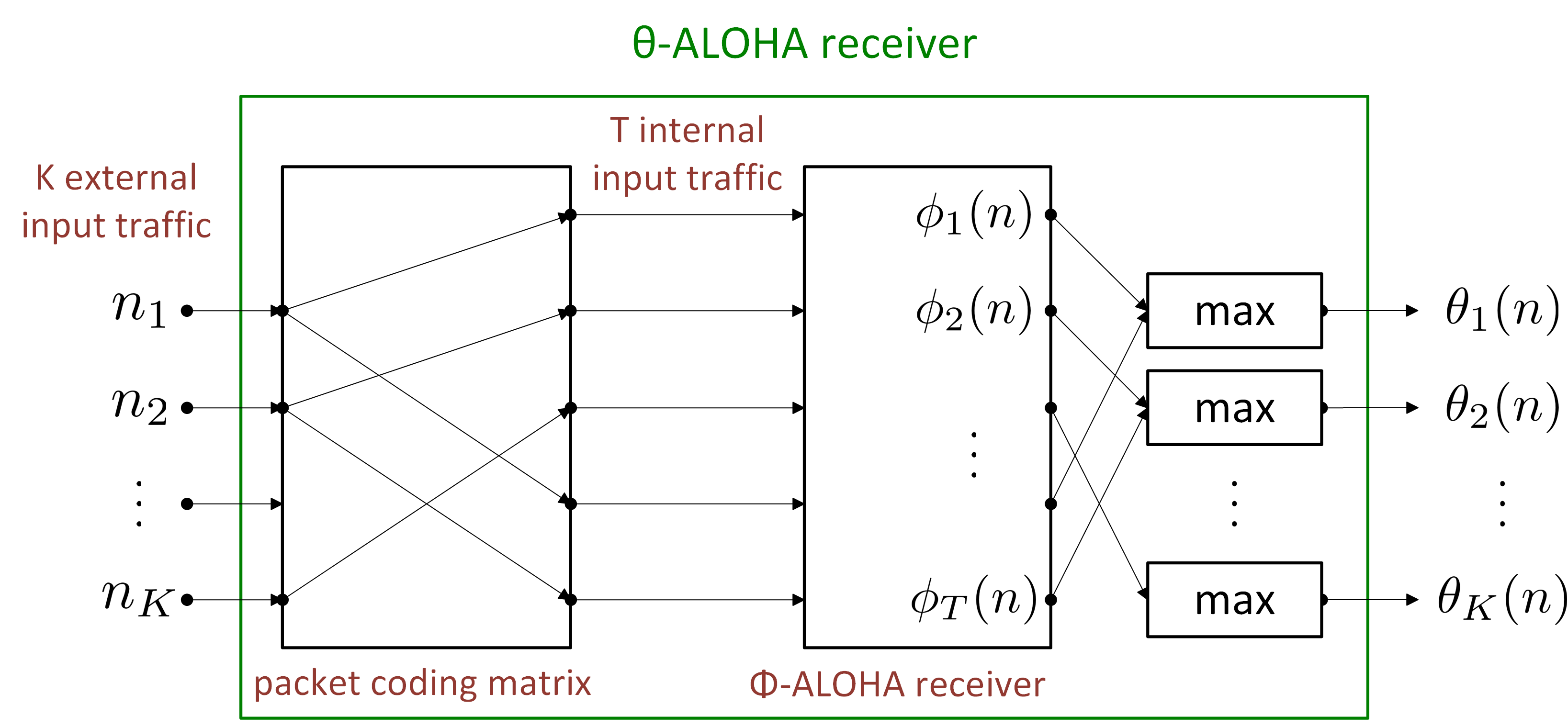
Theorem 13
Interestingly, one can view the system of two cooperative ALOHA receivers in Section III-D as an ALOHA receiver with packet coding. First, an all-or-nothing -ALOHA receiver with classes of input traffic and an all-or-nothing -ALOHA receiver with classes of input traffic can be viewed as an all-or-nothing -ALOHA receiver with classes of input traffic. As the two cooperative ALOHA receivers are subject to the same classes of external input, the coding matrix is simply a concatenation of two identity matrices, i.e., both the first columns of and the last columns of are identity matrices. In view of (57), we have
| (60) |
and thus
| (61) |
It then follows from Lemma 7(vii) that
| (62) |
The result in Theorem 13 then recovers the result in Theorem 9.
We note that if the two receivers are not all-or-nothing ALOHA-receivers, then we have to identify the indices of the packets that are successfully received in order to carry out SIC decoding. As such, the identity in (56) is no longer valid as the class packets that are successfully received in for might not be the same. One interesting example is to consider the two cooperative ALOHA receivers in Section III-D with a single class of input traffic and
| (63) |
When the system is subject to the deterministic load , the decoding result from Theorem 9 is
On the other hand, if we use the decoding method for packet coding and the packet that is successfully received by receiver 1 is different from that by receiver 2, then after the first SIC iteration, the number of packets remained to be decoded is reduced from 3 to 1. After the second iteration, it will be further reduced to 0. This example shows that the decoding result by the method for packet coding might be different from that from Theorem 9 if the two receivers are not all-or-nothing ALOHA-receivers.
For the general setting with joint traffic multiplexing and packet coding, it can be represented by a general bipartite graph with a bi-adjacency matrix . For such a bipartite graph, one can always add an intermediate stage of nodes to form a tripartite graph such that (i) the first part is a bipartite graph with a packet coding matrix , (ii) the second part is a bipartite graph with a traffic multiplexing matrix , and (iii) . One simple way of doing this is to represent each edge in the general bipartite graph by a node in the intermediate stage. By using the results for traffic multiplexing in Theorem 12 and packet coding in Theorem 13, we can then analyze the setting with joint traffic multiplexing and packet coding. We will further illustrate this by considering multiple cooperative -fold ALOHA receivers in the next section.
III-G Multiple cooperative -fold ALOHA receivers
In this section, we show that a system of multiple cooperative -fold ALOHA receivers with joint traffic multiplexing and packet coding is a -ALOHA receiver. Moreover, the success function for such a system can be computed by a max-sum message passing algorithm.
Consider a system with cooperative -fold ALOHA receivers and classes of input traffic through a bi-adjacency matrix . The bi-adjacency matrix is a binary matrix that needs not to satisfy the constraints imposed on a traffic multiplexing matrix or a packet coding matrix. Let , , be the set of receivers associated with class input traffic (the set of nonzero elements in the row of ), and , , be the set of input traffic multiplexed into the receiver (the set of nonzero elements in the column of ). To compute the success function for such a system subject to the deterministic load , we let , where is the number of class packets remained to be decoded in the system after the SIC iteration, , and . Clearly, . Also, let be the number of class that are successfully received by the -fold ALOHA receiver after the iteration. For the first SIC iteration, we know from (53) that if and , and otherwise. From (56), we also know the number of class packets that are remained to be decoded after the first iteration is
| (64) |
. In general, for the SIC iteration, we have
| (65) |
and
| (66) |
. These two recursive equation leads to the max-sum message algorithm in Algorithm 1. Note that Steps 1 and 2 correspond to the computation of in (65), and Step 3 corresponds to the computation of in (66) (as the -fold ALOHA receivers are all-or-nothing ALOHA receivers).
We note there is only a finite number of deterministic loads that need to be computed. To see this, note that if for some , then there are at least packets transmitted to the -fold ALOHA receivers in . As such, no packets can be successfully received by the receivers in , and we can remove all the edges connected to the receive nodes in . Thus, the decoding results are the same for all the deterministic loads with for some . This implies that all the deterministic loads with is equivalent to . As such, there are equivalence classes (as we only need to consider for each ).
Certainly, one can use (25) to compute the throughput of class users subject to a Poisson offered load for such a -ALOHA receiver. However, it is more convenient to compute the throughput of class users from the probabilities of the equivalence classes. Specifically, let is the probability of the deterministic load (equivalence class) subject to a Poisson offered load . For , let
and
For the Poisson distribution with mean , the probabilities for are , . Since the Poisson offered loads from the classes are independent, we have
| (67) |
Using (1) yields
| (68) |
Example 3
(Two cooperative -fold ALOHA receivers) Consider the system with two cooperative -fold ALOHA receivers and three classes of users. Suppose that class 1 (resp. 2) packets are sent to receiver 1 (resp. 2), and class 3 packets are sent to both receivers. The bi-adjacency matrix of the association graph is
| (69) |
As discussed in this section, it is a -ALOHA receiver with the success function being specified in Table I.
| 0 | 0 | 0 | 0 | 0 | 0 |
| 0 | 0 | 1 | 0 | 0 | 1 |
| 0 | 0 | 2 | 0 | 0 | 2 |
| 0 | 0 | 3 | 0 | 0 | 0 |
| 0 | 1 | 0 | 0 | 1 | 0 |
| 0 | 1 | 1 | 0 | 1 | 1 |
| 0 | 1 | 2 | 0 | 1 | 2 |
| 0 | 1 | 3 | 0 | 0 | 0 |
| 0 | 2 | 0 | 0 | 2 | 0 |
| 0 | 2 | 1 | 0 | 2 | 1 |
| 0 | 2 | 2 | 0 | 2 | 2 |
| 0 | 2 | 3 | 0 | 0 | 0 |
| 0 | 3 | 0 | 0 | 0 | 0 |
| 0 | 3 | 1 | 0 | 0 | 1 |
| 0 | 3 | 2 | 0 | 0 | 2 |
| 0 | 3 | 3 | 0 | 0 | 0 |
| 1 | 0 | 0 | 1 | 0 | 0 |
| 1 | 0 | 1 | 1 | 0 | 1 |
| 1 | 0 | 2 | 1 | 0 | 2 |
| 1 | 0 | 3 | 0 | 0 | 0 |
| 1 | 1 | 0 | 1 | 1 | 0 |
| 1 | 1 | 1 | 1 | 1 | 1 |
| 1 | 1 | 2 | 0 | 0 | 0 |
| 1 | 1 | 3 | 0 | 0 | 0 |
| 1 | 2 | 0 | 1 | 2 | 0 |
| 1 | 2 | 1 | 1 | 2 | 1 |
| 1 | 2 | 2 | 0 | 0 | 0 |
| 1 | 2 | 3 | 0 | 0 | 0 |
| 1 | 3 | 0 | 1 | 0 | 0 |
| 1 | 3 | 1 | 1 | 0 | 1 |
| 1 | 3 | 2 | 0 | 0 | 0 |
| 1 | 3 | 3 | 0 | 0 | 0 |
| 2 | 0 | 0 | 2 | 0 | 0 |
| 2 | 0 | 1 | 2 | 0 | 1 |
| 2 | 0 | 2 | 2 | 0 | 2 |
| 2 | 0 | 3 | 0 | 0 | 0 |
| 2 | 1 | 0 | 2 | 1 | 0 |
| 2 | 1 | 1 | 2 | 1 | 1 |
| 2 | 1 | 2 | 0 | 0 | 0 |
| 2 | 1 | 3 | 0 | 0 | 0 |
| 2 | 2 | 0 | 2 | 2 | 0 |
| 2 | 2 | 1 | 0 | 0 | 0 |
| 2 | 2 | 2 | 0 | 0 | 0 |
| 2 | 2 | 3 | 0 | 0 | 0 |
| 2 | 3 | 0 | 2 | 0 | 0 |
| 2 | 3 | 1 | 0 | 0 | 0 |
| 2 | 3 | 2 | 0 | 0 | 0 |
| 2 | 3 | 3 | 0 | 0 | 0 |
| 3 | 0 | 0 | 0 | 0 | 0 |
| 3 | 0 | 1 | 0 | 0 | 1 |
| 3 | 0 | 2 | 0 | 0 | 2 |
| 3 | 0 | 3 | 0 | 0 | 0 |
| 3 | 1 | 0 | 0 | 1 | 0 |
| 3 | 1 | 1 | 0 | 1 | 1 |
| 3 | 1 | 2 | 0 | 0 | 0 |
| 3 | 1 | 3 | 0 | 0 | 0 |
| 3 | 2 | 0 | 0 | 2 | 0 |
| 3 | 2 | 1 | 0 | 0 | 0 |
| 3 | 2 | 2 | 0 | 0 | 0 |
| 3 | 2 | 3 | 0 | 0 | 0 |
| 3 | 3 | 0 | 0 | 0 | 0 |
| 3 | 3 | 1 | 0 | 0 | 0 |
| 3 | 3 | 2 | 0 | 0 | 0 |
| 3 | 3 | 3 | 0 | 0 | 0 |
IV Numerical results
IV-A Two cooperative -fold ALOHA receivers with URLLC traffic and eMBB traffic

In this section, we demonstrate how the framework of Poisson receivers and the framework of ALOHA receivers can be used for providing differentiated services between URLLC traffic and eMBB traffic in uplink transmissions.
IV-A1 Wireless channel model
We consider a wireless channel that is modelled by two cooperative -fold ALOHA receivers in Example 3. There are three classes of input traffic. Class 1 (resp. 2) packets are sent to the first (resp. 2) receiver, and class 3 packets are sent to both receivers (see Figure 7 for an illustration). For such a channel model, it is a -ALOHA receiver with the success function specified in Table I. By using (68), we can compute the success probability functions , , of the induced Poisson receiver. The first two classes are eMBB traffic and the third class is URLLC traffic. Each eMBB packet can be routed to a class 1 packet or a class 2 packet with an equal probability. As a result of the inverse multiplexer in Example 3 of [1], one can use Theorem 2 to model such a channel as a Poisson receiver with two classes of external input traffic, URLLC traffic (external class 1) and eMBB traffic (external class 2). The success probability functions of these two external classes are
| (70) |
IV-A2 Coded random access for a use case
To provide differentiated services between URLLC traffic and eMBB traffic over the wireless channel model in Section IV-A1, we consider the particular use case in Section IV.C of [1] for supporting precise cooperative robotic motion control defined in use case 1 of mobile robots in [38]. For this use case, the message (packet) size of URLLC traffic is 40 bytes, and the transmission time interval (TTI) is 1 ms. According to Table 4.1A-2 in [39], the maximum number of bits of an uplink shared channel (UL-SCH) transport block transmitted within a TTI is 105,528 bits (i.e., 13,191 bytes). As a conservative design, the number of packet transmissions (minislots) within one TTI is set to be 256. As there can be as many as successful packet transmissions in a -fold ALOHA receiver, we set . Thus, for each TTI, there are independent Poisson receivers for the wireless channel model in Section IV-A1. The number of active URLLC users is set to be 50, and each URLLC user uses a coded random access scheme that transmits its packet for times uniformly and independently to the Poisson receivers. On the other hand, each eMBB user is scheduled to transmit exactly one packet in a (randomly assigned) time slot in each TTI. The packets transmitted by URLLC users are superposed with the scheduled eMBB traffic [40] over the wireless channel in Section IV-A1. By viewing each minislot as a Poisson receiver with two classes of input traffic in Section IV-A1, the coded random access scheme corresponds to a system of Poisson receivers with packet coding in Theorem 3, where the degree distribution of URLLC traffic is with (see (5)), and the degree distribution of eMBB traffic is . We note that URLLC transmissions in such a system are decoded first by using the SIC technique. eMBB transmissions that overlap with undecodable URLLC transmissions can be treated as erased or punctured [41] and can be protected by using another layer of error correction codes.
We are interested in addressing the question of how many eMBB users can be admitted to the system so that the packet error probability of URLLC traffic is less than .
In Figure 8, we show the theoretical results and the simulation results for and . Each data point for the estimated error probability is obtained by averaging over 100,000 independent runs. Also, we set the number of iterations for SIC to be 100 (). As shown in Figure 8, our theoretical results match extremely well with the simulation results except for those data points with extremely small error probabilities. For , the 1-fold ALOHA receiver is the simply the SA system considered in Section IV.C of [1]. One can see from this figure that the performance of the 2-fold ALOHA receivers is significantly better than that of the SA system. In particular, the number of eMBB users can be admitted to the system is increased from 194 for the system with two 1-fold ALOHA receivers to 292 for the system with two 2-fold ALOHA receivers (while keeping the error probability of URLLC packets lower than ).
IV-B Rayleigh block fading channel with URLLC traffic and eMBB traffic
In this section, we consider the Rayleigh block fading channel with capture in Section II-B. Such a wireless channel can be modelled by a Poisson receiver with a single class of input in (19). By using Theorem 2 for Poisson receivers with packet routing, such a wireless channel can be extended to a Poisson receiver with two classes of input traffic. The success probability functions for these two classes of input traffic are as follows:
To provide differentiated services between URLLC traffic and eMBB traffic, we use the coded random access scheme with minislots as described in Section IV-A2. We assume that the channel gains for these two classes in minislots are independent, and thus such a system corresponds to a system of Poisson receivers with packet coding in Theorem 3. In our experiments, we use the same parameters as those in Section IV-A2, i.e., the number of minislots , the number of URLLC users , the number of SIC iterations , the degree distribution of URLLC traffic , and the degree distribution of eMBB traffic . For the Rayleigh block fading channel, we set and . As in Section IV-A2, each data point is obtained by averaging over 100,000 independent runs. In Figure 9, we show the theoretical results and the simulation results for the effect of the number of eMBB users on the error probability of URLLC users in the Rayleigh block fading channel with capture. Once again, our theoretical results match extremely well with the simulation results. The number of eMBB users can be admitted to the system is roughly 58 while keeping the error probability of URLLC packets lower than .
V Conclusion
In this paper, we developed a deterministic framework of -ALOHA receivers that can be incorporated into the probabilistic framework of Poisson receivers for analyzing coded multiple access with SIC. Like the theory of network calculus, there are various algebraic properties for several operations on functions, including minimum , composition , closure , and complement . As such, small ALOHA receivers can be used as building blocks for constructing a large ALOHA receiver. In particular, we showed various closure properties of ALOHA receivers, including (i) ALOHA receivers in tandem, (ii) cooperative receivers, (iii) ALOHA receivers with traffic multiplexing, and (iv) ALOHA receivers with packet coding. As an illustrating example, we computed/simulated the numerical results of a system that uses two cooperative -fold ALOHA receivers with packet coding to provide differentiated services between URLLC traffic and eMBB traffic. The theoretical results in this example match extremely well with the simulation results (except for those data points with extremely small error probabilities).
References
- [1] C.-H. Yu, L. Huang, C.-S. Chang, and D.-S. Lee, “Poisson receivers: a probabilistic framework for analyzing coded random access,” arXiv preprint arXiv:2008.07561, 2020.
- [2] C.-P. Li, J. Jiang, W. Chen, T. Ji, and J. Smee, “5g ultra-reliable and low-latency systems design,” in Networks and Communications (EuCNC), 2017 European Conference on. IEEE, 2017, pp. 1–5.
- [3] M. Bennis, M. Debbah, and H. V. Poor, “Ultra-reliable and low-latency wireless communication: Tail, risk and scale,” arXiv preprint arXiv:1801.01270, 2018.
- [4] P. Popovski, Č. Stefanović, J. J. Nielsen, E. De Carvalho, M. Angjelichinoski, K. F. Trillingsgaard, and A.-S. Bana, “Wireless access in ultra-reliable low-latency communication (urllc),” IEEE Transactions on Communications, vol. 67, no. 8, pp. 5783–5801, 2019.
- [5] E. Casini, R. De Gaudenzi, and O. D. R. Herrero, “Contention resolution diversity slotted aloha (crdsa): An enhanced random access schemefor satellite access packet networks,” IEEE Transactions on Wireless Communications, vol. 6, no. 4, 2007.
- [6] G. Liva, “Graph-based analysis and optimization of contention resolution diversity slotted aloha,” IEEE Transactions on Communications, vol. 59, no. 2, pp. 477–487, 2011.
- [7] K. R. Narayanan and H. D. Pfister, “Iterative collision resolution for slotted aloha: An optimal uncoordinated transmission policy,” in Turbo Codes and Iterative Information Processing (ISTC), 2012 7th International Symposium on. IEEE, 2012, pp. 136–139.
- [8] E. Paolini, G. Liva, and M. Chiani, “Random access on graphs: A survey and new results,” in Signals, Systems and Computers (ASILOMAR), 2012 Conference Record of the Forty Sixth Asilomar Conference on. IEEE, 2012, pp. 1743–1747.
- [9] D. Jakovetić, D. Bajović, D. Vukobratović, and V. Crnojević, “Cooperative slotted aloha for multi-base station systems,” IEEE Transactions on Communications, vol. 63, no. 4, pp. 1443–1456, 2015.
- [10] Č. Stefanović and D. Vukobratović, “Coded random access,” in Network Coding and Subspace Designs. Springer, 2018, pp. 339–359.
- [11] R. Hoshyar, F. P. Wathan, and R. Tafazolli, “Novel low-density signature for synchronous cdma systems over awgn channel,” IEEE Transactions on Signal Processing, vol. 56, no. 4, pp. 1616–1626, 2008.
- [12] H. Nikopour and H. Baligh, “Sparse code multiple access,” in Personal Indoor and Mobile Radio Communications (PIMRC), 2013 IEEE 24th International Symposium on. IEEE, 2013, pp. 332–336.
- [13] Z. Yuan, G. Yu, W. Li, Y. Yuan, X. Wang, and J. Xu, “Multi-user shared access for internet of things,” in Vehicular Technology Conference (VTC Spring), 2016 IEEE 83rd. IEEE, 2016, pp. 1–5.
- [14] S. Chen, B. Ren, Q. Gao, S. Kang, S. Sun, and K. Niu, “Pattern division multiple access—a novel nonorthogonal multiple access for fifth-generation radio networks,” IEEE Transactions on Vehicular Technology, vol. 66, no. 4, pp. 3185–3196, 2017.
- [15] O. Ordentlich and Y. Polyanskiy, “Low complexity schemes for the random access gaussian channel,” in 2017 IEEE International Symposium on Information Theory (ISIT). IEEE, 2017, pp. 2528–2532.
- [16] C.-S. Chang, D.-S. Lee, and C. Wang, “Asynchronous grant-free uplink transmissions in multichannel wireless networks with heterogeneous qos guarantees,” IEEE/ACM Transactions on Networking, vol. 27, no. 4, pp. 1584–1597, 2019.
- [17] Y. Liu, Y. Deng, M. Elkashlan, A. Nallanathan, and G. K. Karagiannidis, “Analyzing grant-free access for urllc service,” arXiv preprint arXiv:2002.07842, 2020.
- [18] K. Andreev, E. Marshakov, and A. Frolov, “A polar code based tin-sic scheme for the unsourced random access in the quasi-static fading mac,” arXiv preprint arXiv:2005.06899, 2020.
- [19] R. Gallager, “Low-density parity-check codes,” IRE Transactions on information theory, vol. 8, no. 1, pp. 21–28, 1962.
- [20] Č. Stefanović, M. Momoda, and P. Popovski, “Exploiting capture effect in frameless aloha for massive wireless random access,” in 2014 IEEE Wireless Communications and Networking Conference (WCNC). IEEE, 2014, pp. 1762–1767.
- [21] F. Clazzer, E. Paolini, I. Mambelli, and Č. Stefanović, “Irregular repetition slotted aloha over the rayleigh block fading channel with capture,” in 2017 IEEE International Conference on Communications (ICC). IEEE, 2017, pp. 1–6.
- [22] R. L. Cruz, “A calculus for network delay. i. network elements in isolation,” IEEE Transactions on information theory, vol. 37, no. 1, pp. 114–131, 1991.
- [23] ——, “A calculus for network delay. ii. network analysis,” IEEE Transactions on information theory, vol. 37, no. 1, pp. 132–141, 1991.
- [24] C.-S. Chang, Performance guarantees in communication networks. Springer Science & Business Media, 2012.
- [25] J.-Y. Le Boudec and P. Thiran, Network calculus: a theory of deterministic queuing systems for the internet. Springer Science & Business Media, 2001, vol. 2050.
- [26] S. Mao and S. S. Panwar, “A survey of envelope processes and their applications in quality of service provisioning,” IEEE Communications Surveys & Tutorials, vol. 8, no. 3, pp. 2–20, 2006.
- [27] Y. Jiang and Y. Liu, Stochastic network calculus. Springer, 2008, vol. 1.
- [28] M. Fidler, “Survey of deterministic and stochastic service curve models in the network calculus,” IEEE Communications surveys & tutorials, vol. 12, no. 1, pp. 59–86, 2010.
- [29] F. Baccelli, G. Cohen, G. J. Olsder, and J.-P. Quadrat, “Synchronization and linearity: an algebra for discrete event systems,” 1992.
- [30] A. K. Parekh and R. G. Gallager, “A generalized processor sharing approach to flow control in integrated services networks: the single-node case,” IEEE/ACM transactions on networking, vol. 1, no. 3, pp. 344–357, 1993.
- [31] H. Sariowan, R. L. Cruz, and G. C. Polyzos, “Sced: A generalized scheduling policy for guaranteeing quality-of-service,” IEEE/ACM Transactions on networking, vol. 7, no. 5, pp. 669–684, 1999.
- [32] E. Paolini, C. Stefanović, G. Liva, and P. Popovski, “Coded random access: applying codes on graphs to design random access protocols,” IEEE Communications Magazine, vol. 53, no. 6, pp. 144–150, 2015.
- [33] A. Munari, F. Clazzer, and G. Liva, “Multi-receiver aloha systems-a survey and new results,” in Communication Workshop (ICCW), 2015 IEEE International Conference on. IEEE, 2015, pp. 2108–2114.
- [34] M. Luby, M. Mitzenmacher, and M. A. Shokrollahi, “Analysis of random processes via and-or tree evaluation,” in SODA, vol. 98, 1998, pp. 364–373.
- [35] M. Luby, M. Mitzenmacher, A. Shokrollah, and D. Spielman, “Analysis of low density codes and improved designs using irregular graphs,” in Proceedings of the thirtieth annual ACM symposium on Theory of computing, 1998, pp. 249–258.
- [36] T. J. Richardson and R. L. Urbanke, “The capacity of low-density parity-check codes under message-passing decoding,” IEEE Transactions on Information Theory, vol. 47, no. 2, pp. 599–618, 2001.
- [37] N. Abramson, “The aloha system: another alternative for computer communications,” in Proceedings of the November 17-19, 1970, fall joint computer conference. ACM, 1970, pp. 281–285.
- [38] 3GPP, “Service requirements for cyber-physical control applications in vertical domains,” 3rd Generation Partnership Project (3GPP), Technical Specification (TS) 22.104, 03 2019, version 16.1.0. [Online]. Available: https://portal.3gpp.org/desktopmodules/Specifications/SpecificationDetails.aspx?specificationId=3528
- [39] ——, “Evolved Universal Terrestrial Radio Access (E-UTRA); User Equipment (UE) radio access capabilities,” 3rd Generation Partnership Project (3GPP), Technical Specification (TS) 36.306, 06 2019, version 15.5.0. [Online]. Available: https://portal.3gpp.org/desktopmodules/Specifications/SpecificationDetails.aspx?specificationId=2434
- [40] A. Anand, G. De Veciana, and S. Shakkottai, “Joint scheduling of urllc and embb traffic in 5g wireless networks,” IEEE/ACM Transactions on Networking, vol. 28, no. 2, pp. 477–490, 2020.
- [41] P. Popovski, K. F. Trillingsgaard, O. Simeone, and G. Durisi, “5g wireless network slicing for embb, urllc, and mmtc: A communication-theoretic view,” IEEE Access, vol. 6, pp. 55 765–55 779, 2018.
![[Uncaptioned image]](2009.03145v1/THLiu.jpg) |
Tzu-Hsuan Liu received the B.S. degree in communication engineering from National Central University, Taoyuan, Taiwan (R.O.C.), in 2018. She is currently pursuing the M.S. degree in the Institute of Communications Engineering, National Tsing Hua University, Hsinchu, Taiwan (R.O.C.). Her research interest is in 5G wireless communication. |
![[Uncaptioned image]](2009.03145v1/chehaoyu.jpg) |
Che-Hao Yu received his B.S. degree in mathematics from National Tsing-Hua University, Hsinchu, Taiwan (R.O.C.), in 2018, and the M.S. degree in communications engineering from National Tsing Hua University, Hsinchu, Taiwan (R.O.C.), in 2020. His research interest is in 5G wireless communication. |
![[Uncaptioned image]](2009.03145v1/YJLin.jpg) |
Yi-Jheng Lin received his B.S. degree in electrical engineering from National Tsing Hua University, Hsinchu, Taiwan, in 2018. He is currently pursuing the Ph.D. degree in the Institute of Communications Engineering, National Tsing Hua University, Hsinchu, Taiwan. His research interests include wireless communication and cognitive radio networks. |
![[Uncaptioned image]](2009.03145v1/cschang.png) |
Cheng-Shang Chang (S’85-M’86-M’89-SM’93-F’04) received the B.S. degree from National Taiwan University, Taipei, Taiwan, in 1983, and the M.S. and Ph.D. degrees from Columbia University, New York, NY, USA, in 1986 and 1989, respectively, all in electrical engineering. From 1989 to 1993, he was employed as a Research Staff Member with the IBM Thomas J. Watson Research Center, Yorktown Heights, NY, USA. Since 1993, he has been with the Department of Electrical Engineering, National Tsing Hua University, Taiwan, where he is a Tsing Hua Distinguished Chair Professor. He is the author of the book Performance Guarantees in Communication Networks (Springer, 2000) and the coauthor of the book Principles, Architectures and Mathematical Theory of High Performance Packet Switches (Ministry of Education, R.O.C., 2006). His current research interests are concerned with network science, big data analytics, mathematical modeling of the Internet, and high-speed switching. Dr. Chang served as an Editor for Operations Research from 1992 to 1999, an Editor for the IEEE/ACM TRANSACTIONS ON NETWORKING from 2007 to 2009, and an Editor for the IEEE TRANSACTIONS ON NETWORK SCIENCE AND ENGINEERING from 2014 to 2017. He is currently serving as an Editor-at-Large for the IEEE/ACM TRANSACTIONS ON NETWORKING. He is a member of IFIP Working Group 7.3. He received an IBM Outstanding Innovation Award in 1992, an IBM Faculty Partnership Award in 2001, and Outstanding Research Awards from the National Science Council, Taiwan, in 1998, 2000, and 2002, respectively. He also received Outstanding Teaching Awards from both the College of EECS and the university itself in 2003. He was appointed as the first Y. Z. Hsu Scientific Chair Professor in 2002. He received the Merit NSC Research Fellow Award from the National Science Council, R.O.C. in 2011. He also received the Academic Award in 2011 and the National Chair Professorship in 2017 from the Ministry of Education, R.O.C. He is the recipient of the 2017 IEEE INFOCOM Achievement Award. |
![[Uncaptioned image]](2009.03145v1/dslee.png) |
Duan-Shin Lee (S’89-M’90-SM’98) received the B.S. degree from National Tsing Hua University, Taiwan, in 1983, and the MS and Ph.D. degrees from Columbia University, New York, in 1987 and 1990, all in electrical engineering. He worked as a research staff member at the C&C Research Laboratory of NEC USA, Inc. in Princeton, New Jersey from 1990 to 1998. He joined the Department of Computer Science of National Tsing Hua University in Hsinchu, Taiwan, in 1998. Since August 2003, he has been a professor. He received a best paper award from the Y.Z. Hsu Foundation in 2006. He served as an editor for the Journal of Information Science and Engineering between 2013 and 2015. He is currently an editor for Performance Evaluation. Dr. Lee’s current research interests are network science, game theory, machine learning and high-speed networks. He is a senior IEEE member. |
Appendix A
It this section, we show the derivation of (II-B).