∎
Efficient Projection Algorithms onto the Weighted Ball
Abstract
Projected gradient descent has been proved efficient in many optimization and machine learning problems. The weighted ball has been shown effective in sparse system identification and features selection. In this paper we propose three new efficient algorithms for projecting any vector of finite length onto the weighted ball. The first two algorithms have a linear worst case complexity. The third one has a highly competitive performances in practice but the worst case has a quadratic complexity. These new algorithms are efficient tools for machine learning methods based on projected gradient descent such as compress sensing, feature selection. We illustrate this effectiveness by adapting an efficient compress sensing algorithm to weighted projections. We demonstrate the efficiency of our new algorithms on benchmarks using very large vectors. For instance, it requires only 8 ms, on an Intel I7 3rd generation, for projecting vectors of size .
1 Introduction
Looking for sparsity appears in many machine learning applications, such as biomarker identification in biology abeel2009robust; he2010stable, or the recovery of sparse signals in compressed sensing donoho2006compressed. For example consider the problem of minimizing a common reconstruction loss function. In addition consider constraining the number of non-zero components ( norm) of the learned vector to be lower than a given sparsity value:
A solution of this generic problem will use only a subset of size lower than of the components of leading to the best reconstruction error. This implies that solving this problem and varying the value allows us to manage sparsity with a fine grain. Unfortunately, this problem is generally strictly nonconvex and very difficult to solve natarajan1995sparse. Hence a common solution is to constrain the norm of the vector instead tibshirani96; donoho03, or one of its modified versions slavakis10; kopsinis2010online; bogdan2015slope. More specifically, the weighted ball has been proven to have strong properties for finding or recovering sparse vectors candes2008enhancing; slavakis10. To this purpose, it is crucially important to have simple algorithms to work with the weighted ball during the optimization process. Several methods in machine learning are based on projected gradient descent for their optimization part, for example by iterating between gradient updates and ball projections duchi. The goal of this paper is to help the application of projected gradient descent methods for solving sparse machine learning problems by working with the weighted ball. Unfortunately, efficiently applying projected gradient descent requires an efficient projection algorithm. For the basic ball, many projection algorithms have been proposed michelot86; van08; kiwiel08; condat; perez19, but in the context of the weighted ball, only few works have been done slavakis10.
In this paper, we propose three efficient projection algorithms by generalizing works made for the basic (i.e. non weighted) ball to its generalization, the weighted ball. We start by giving a proof of existence of the threshold value () allowing efficient projection algorithms as for the basic ball held74. Using this threshold, we propose three efficient algorithms. First, - iteratively approximates using a pivot-based algorithm. It Splits the vector in two sub-vectors at each iteration and has quadratic worst case complexity, but is near linear in practice. Second, - and - , two algorithms based on a bucket decomposition of the vector that efficiently detects components that will be zero in the projection. These two ones have linear worst case complexity. We propose an experimental protocol using randomly generated high dimensional () vectors to show the performances of our algorithm. We then adapt the sparse vector recovery framework from trzasko08 to the proposed projection algorithms and show the efficiency and simplicity of the model. The paper starts with the definitions of the projection onto the and weighted balls, and highlights the need of finding the value. In the projection section, the algorithm - is first defined and the algorithms - and - are later defined. In the experiments section, an evaluation of the time performances shows that the proposed algorithms are order of magnitude faster than current projection methods, and then that they can be used to adapt existing machine-learning frameworks. Finally, the proofs required for the proposed algorithms are given and followed by the conclusion.
2 Definitions of the Projections
ball
Given a vector and a real , we aim at computing its projection onto the ball of radius :
| (1) |
where . The projection is defined by
| (2) |
where is the Euclidean norm. As shown in duchi and revisited in condat, the projection onto the ball can be derived from the projection onto the simplex :
| (3) |
Let the sign function defined as if , if and otherwise, for any real value . The projection of onto the ball is given by the following formula:
| (4) |
where with is the projection of onto . An important property has been established to compute this projection. It was shown held74 that there exists a unique such that
| (5) |
The projection is almost equivalent to a thresholding operation. The main difficulty is to compute quickly the threshold for any vector . Let be the th largest value of such that . It is interesting to note that (5) involves that . Let be the support of , i.e., . Then,
It follows that where is the number of elements of . The following property allows us to compute the threshold . Let
| (6) |
for any . Then, it was shown that where
| (7) |
Looking for , or equivalently , allows us to find immediately the threshold . The most famous algorithm to compute the projection, which has been presented in held74, is based on (7). It consists in sorting the values and then finding the first value satisfying (7). A possible implementation is given in Algorithm 1. The worst case complexity of this algorithm is . Several other methods have been proposed michelot86; van08; kiwiel08; condat; perez19, outperforming this simple approach.
for do
Weighted ball
Given a vector , a vector , 11 1 We can consider instead of without loss of generality since the associated entries of y will be present in the projection, and do not influence the processing of the rest of the projection. for all , and a real , we aim at computing its projection onto the weighted ball of radius :
| (8) |
The projection is defined by
| (9) |
where is the Euclidean norm.
As for the classical ball, the weighted projection operator can be derived from the weighted simplex projection slavakis10:
| (10) |
The projection of onto the weighted ball is given by the following formula:
| (11) |
where with is the projection of onto . Once again, the fast computation of the projection for any vector is of utmost importance.
Let the vector , the vector , for all , and a real , if , then there exists a unique such that
| (12) |
The proof is given in the proof section of this paper, and is used to derive three projection algorithms. These algorithms are generalizations of the current state-of-the-art algorithms for ball projection condat; perez19. The main difficulty is to compute quickly the threshold for any vector . Let be the vector such that
| (13) |
Let be the th largest value of such that . Let (resp. ) be the th entry of such that . is a permutation of with respect to the order of . It is interesting to note that equation (12) implies that . Let be the support of , i.e., . Then,
It follows that
| (14) |
The following property compute the threshold .
| (15) |
for any . Then, we have shown in the proof section that where
| (16) |
Looking for , or equivalently , gives us immediately the threshold .
A direct algorithm to compute this projection, which is a generalization of held74, is based on (16), and is given in Algorithm 2. This algorithm starts by sorting the values according to , and then searches for the index. Note that once sorted, finding is easily done by starting from the largest value. That is why Algorithm 2 does not need more steps as in slavakis10; kopsinis2010online.
Permutation
for do
3 Efficient Projection
Many works have focused on designing efficient algorithms for finding given and michelot86; kiwiel08; van08; condat; perez19. In this section, given , , and , we propose to generalize some of these efficient algorithms to find the projection onto the weighted ball . Specifically, we generalize the methods from condat; perez19 that we respectively name and . Both of these methods are looking for the value such that the projection is defined by equation (5).
For the weighted ball, we are looking for the value such that the projection is given by equation (12). As for the basic ball, the weighted ball algorithms are looking for and from equation (16). Let . If is sorted in increasing order, then finding can be easily done by iteratively processing , with until , as shown in Algorithm 2. A projection algorithm using as a first iteration a sort has already been proposed slavakis10. But most of the time is not sorted, and sorting is the exact operation that we want to avoid because of its time complexity, and that often, we are looking for sparse solutions, thus only a subset of the values of will remain relevant. This section is split into two parts. The first one is a generalization of the algorithm condat. The second one is a generalization of the algorithm perez19.
3.1 - Algorithm
In this section we propose a generalization of the algorithm. The proposed algorithm is composed of three points that we name pivot, lower bound extraction and online filtering, and are described in the next paragraphs. The idea of the algorithm is the following, at each iteration, the vector is split into two sub-vectors, using a pivot value, and determine which sub-vector contains (pivot part). In the mean time, a fine grain lower bound is defined as a pivot for an efficient splitting (lower bound part). Finally, the algorithm discards on the fly values that are provably not part of (online filtering part).
Pivot It is often considered that for regular amount of data, the quicksort algorithm is the fastest sort thomas2001. The quicksort algorithm splits the data into two partitions by using a pivot value. Values smaller than the pivot go into the first partition, others in the second. The process is then applied recursively to both partitions. In the context of the basic simplex projection, using a pivot like algorithm led to some of the most efficient algorithms kiwiel08; duchi; michelot86; condat. From equation (14), we can notice that the value only requires the knowledge about elements of the set , but not that this set is ordered. Such a remark gives a hint in why partitioning instead of sorting could be beneficial. Consider , note that to get and only one pass over the vector is required. One can partition into and by putting the elements smaller (resp larger) than from . Consider that the size of is (i.e. it contains entries), then we can easily compute . If , then . If this condition is true, this implies that we can stop the processing of because . If the condition is false, if , then , then we know that . Using this knowledge, we can continue the processing of .
Lower bound as pivot The choice for the pivot is of utmost importance for the global running time, we can easily show that the worst case complexity is . As for the basic simplex, one could seek for the median pivot kiwiel08. From a complexity point of view, this could be an improvement, but our goal is not to partition equitably the data, but to efficiently find . Instead, we will seek for a pivot which is a lower bound of .
Let be any sub-sequence of . Then the value
| (17) |
is a lower bound of . The proof can be found at the end of this paper.
Using as a pivot implies that elements of can always be discarded.
Proof. If we use as a threshold value, and by definition of a lower bound, we have:
| (18) |
If , it implies that , which also implies that . Consider the algorithm iterating between the following step: Step 1) Set . Step 2) remove elements of which are smaller than . This algorithm will converge to a state where no element can be removed anymore. This state implies that the resulting vector is .
Online Filtering Another optimization of this algorithm is the following, the pivot value does not need to wait until the end of step 2) before being updated, but can be updated after every element of is read. Such an interactive update requires us to divide the algorithm in two parts.
The first part is the first pass over , where we do not have any knowledge about . Let initialize and the pivot by . Consider that we are processing the th element of , which implies that we have already processed all the elements in []. From these elements, we have built a sub-sequence , and an associated pivot . If we have , then, as before, we can discard this element. Otherwise, if , then we can add to because is potentially larger than . Once is updated, we can update incrementally without waiting for the pass to be over, and then process the th element of .
For the second part, we have hopefully already discarded several elements of , and more importantly, we have a set containing elements that are potentially larger than . In addition, we have the associated pivot , which is processed with respect to all the elements in . Consider that we pass over the elements of , if , then we can remove from , and update accordingly. Note that just like for the first part, this can be done incrementally. When no more element can be removed from , the algorithm finished and . A possible implementation is given in Algorithm 3.
In the same fashion as condat, we have incorporated a refinement. During the first iteration, while processing the th element, when the current pivot value is smaller than the one defined by the current value , then will become the new basis. To do that, an additional set is required and a cleanup step which ensures that contains all the elements larger than before the second part of the algorithm. Note that the proposed algorithm works on the permuted space of without using for the calculation of and , which is a major difference with the non-weighted version.
for do
for do
3.2 - Algorithm
In this section, we present the - algorithm, which is a generalization of the linear time simplex projection perez19. - fundamental idea is to recursively split vector into ordered sub-vectors (say buckets) with and , while looking for . We say that the sub-vectors are ordered in the sense that all elements of are smaller than the ones of for all . The depth, or number of recursive splitting is . In the description of - , from the two sub-vectors and , only one of them was re-used at the next iteration. In the - algorithm, only one of the buckets will be re-used at the next iteration. Such a fine grain gives us three possible states for the buckets, , , . Only one bucket will be in the uncertainty state (), this is the bucket that will be re-used.
We define here the different components of the - algorithm. For any level , consider the interval defined by
| (19) |
with (resp. ) the minimum (resp. maximum) element of sub-vector .
Consider a partition of into ordered sub-intervals ,…, . Let be the bucketing function such that when the real value belongs to . The bucket is split into ordered sub-vectors such that
- 1.
,
- 2.
,
- 3.
for all ,
with the convention . We get at any level because of the definition of . The fact that follows from the fact that equal values of necessarily belongs to the same bucket.
For any ,
| (20) |
| (21) |
| (22) |
are cumulative sums of all the buckets discarded because we know they belong to from previous iterations, and all the larger or equal buckets of the iteration . Both of these values will be used for incrementally processing , equation (15). More precisely, we define:
| (23) |
Let be the largest value such that is not empty. If , then and we can discard all the buckets with and continue to the next iteration, since . Otherwise, if , then and we can continue processing the other buckets. Let be the largest value such that is not empty and . We know that for all , , and that for all , . Thus we can safely go to the next iteration, considering only . Note that if , then such a value does not exist, and at the first iteration we can stop.
From the definition of (19), we can show that the size of the bucket is strictly decreasing. Let be the iteration where is the minimum value of a bucket . Let be the largest value, strictly lower than , such that is not empty. We have:
| (24) |
Such a condition, from equation (16), implies that . The complexity of the - algorithm is highly dependent of the bucketing function , and using equation (19), we can easily show that the worst case complexity is bound by . Following the same idea as perez19, we can use a bucketing function based on the numbers encoding in nowadays computers. Such a function, at each iteration, choose to partition the numbers with respect to their th byte, in the same fashion as the Radix sort thomas2001. Using such a bucketing function loose the property of equation (19), but the advantage is that the complexity becomes linear . An implementation is given in Algorithm 4.
1 for do
for do
Filtering The advantage of algorithm - is to discard values that are known to be already dominated by an incrementally updated lower bound of . In - , we can easily use the exact same lower bound, by keeping its process in parallel of the processing of the buckets. Moreover, thanks to the bucketization, we can also have another lower bound. When we are processing bucket at iteration , then is another, pretty good lower bound of . Note that this value should be directly available, because it was required to process the previous bucket. Finally, the filtering consists in removing values that are lower than one of our lower bounds.
4 Experimental evaluation
In these experiments, we reproduced the experiments from perez19 by defining random vectors of size varying between and , using either uniform or Gaussian distributions. We generated 500 vectors for each experiment and ran each algorithm independently, and extracted their mean times. We show here the performances of the proposed algorithms, - , and - and - against the existing algorithm - slavakis10 Algorithm 1, implemented using an efficient quick-sort procedure. The difference between - and - is the use or not of the filtering improvement. All the algorithms are implemented in C, and run on a I7 3rd generation. All source codes are available online22 2 Link hidden.
Uniform We start our experiments with Figure 4. This figure shows that when a uniform random distribution is used for vector , the time needed for projecting the vector grows linearly for all methods as a function of the vector size. Moreover, the proposed algorithms seem to perform order of magnitude faster than -, which is already a faster algorithm than the state of the art. The second plot of Figure 4 shows the impact of the radius for the projection time. It is interesting to note that while all proposed methods outperform the sorting scheme, when the radius becomes too large, the cost of filtering become larger than the gain it can bring, because less values are discarded.
Gaussian Figure 6 (top) shows that the time seems to grow linearly with , the size of vector . Moreover, the - and - algorithms perform better. Figure 6 (bottom) shows that first, when the radius is small or unit, the filtering algorithms are the most efficient, but the more the radius grows, the less they are, and the classical bucket become the best one. Such a result may imply that in function of the radius size, one should choose to use the filtering or not in the - algorithms. Figures 5 shows the different results for the filtered algorithms only, since their running times are order of magnitude faster. As we can see, they behave similarly in most of the cases, which may imply that the larger cuts in the search are induced by the filtering scheme, rather than the splitting scheme.
Discussion Differences in terms of running time between - and - are relatively small in practice. From a theoretical point of view, both of these algorithms take advantage of the filtering. Thus implementing both algorithms in a projected gradient descent solver would be useless. We made the choice of designing these two algorithms because they represent some of the current best state of the art algorithms for the ball. From our point of view, only the - algorithm should be implemented because of its efficiency and complexity guaranties.
5 Variables Selection
In signal reconstruction and variables selection, the non-smooth () regularization has proven efficient in finding sparse solutions. Consider the problem of minimizing a quadratic reconstruction error subject to the regularization, .
| (25) |
where , , and is the penalty parameter.
A popular method to solve this problem is to use the iteratively reweighted minimization (IRL1) candes2008enhancing; chartrand2008iteratively; chen2010convergence; chen2014convergence. An application of IRL1 to problem (25) can be
| (26) |
with the weight , and is defined by the previous iterates by
| (27) |
where .
Using the weighted ball projection algorithms proposed in this paper, solving (26) can be done easily. We propose to use the following algorithm, based on trzasko08, we start with randomly defined. We set , which is equivalent to solving the LASSO problem. Then, we smoothly decrease , and iteratively solve an IRL1 problem such as (26) with a fixed . A possible implementation of this algorithm is in Algorithm 5. We call this algorithm Smooth Iterative Reweighted ball Projections (SIRL1).
Reconstruction results
We show in the section the reconstruction efficiency of the SIRL1, which is a direct application of having an efficient projection onto the weighted L1 ball. We reproduce here part of the experimental protocol of candes2008enhancing. We compare the reconstruction error and the sparsity against the state of the art LASSO algorithm and the projection based (PC) version of candes2008enhancing. In this experiment, is the number of rows, the number of columns and the real number of non-zero components of the solution. First, table 3 shows some results on the reconstruction of sparse vectors with sparsity of 5, 15, 30 non-zero values over 100 values. As we can see, The reconstruction accuracy and the sparsity is rapidly found with even a small number of different . Moreover, because of the smoothness induced by , even if the number of iterations is larger in (a=5,) compared to (a=5,), the running time is slower.
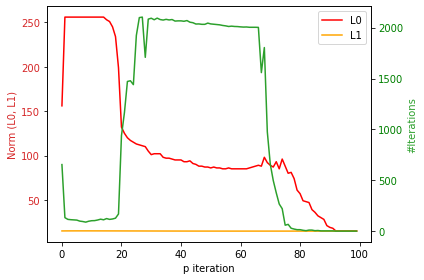
A look at the impact of the smoothness between the values of is given in Table 3. We can see that less than 3 iterations over may be too small, and that more than 5 in this example seem to be useless. But one must be careful with the smoothness, we tried to push the smoothness to 100 iterations over , the results are in Fig 1. As we can see, the number of iterations between and is high, while the L0 norm is not impacted. We were able to see this kind of results in different settings we set, with larger , and . Finaly, the radius is one of the most important parameter of this algorithm, it’s impact can be seen on table 3. As it is expected, a radius smaller than the number of non-zero components has a bad impact on the reconstruction, but it is interesting to see that less iterations seem to be required to solve these problems than for larger values of the radius. Finally, the results we obtained are coherent with the results obtained in trzasko08, which validates the inverted model we used.
| Algo | L0 | L1 | rec | time | #it | a |
|---|---|---|---|---|---|---|
| Lasso | 5 | 5.00 | 1.00 | 0.0029 | 11 | 5.00 |
| PC | 5 | 4.86 | 4.82 | 1.1295 | 3880 | 5.00 |
| 5 | 5.22 | 0.00 | 0.2542 | 2107 | 5.00 | |
| 5 | 5.22 | 0.00 | 0.1844 | 2176 | 5.00 | |
| Lasso | 151 | 15.00 | 0.01 | 0.0163 | 159 | 15.00 |
| PC | 256 | 14.80 | 0.00 | 0.9570 | 307 | 15.00 |
| 15 | 14.80 | 0.01 | 0.3580 | 4909 | 15.00 | |
| 15 | 14.80 | 0.00 | 0.3790 | 5201 | 15.00 | |
| Lasso | 146 | 30.00 | 0.05 | 0.0223 | 240 | 30.00 |
| PC | 256 | 27.73 | 0.00 | 0.0477 | 352 | 30.00 |
| 30 | 27.73 | 0.00 | 0.1563 | 2053 | 30.00 | |
| 30 | 27.73 | 0.00 | 0.5103 | 7131 | 30.00 |
| L0 | L1 | rec | time | #it | a | |
|---|---|---|---|---|---|---|
| 156 | 15.00 | 0.00 | 0.0580 | 655 | 15.00 | 1 |
| 15 | 14.76 | 0.15 | 0.0600 | 796 | 15.00 | 2 |
| 15 | 14.80 | 0.01 | 0.3429 | 4909 | 15.00 | 3 |
| 15 | 14.80 | 0.00 | 0.3770 | 5201 | 15.00 | 5 |
| 15 | 14.80 | 0.00 | 0.4386 | 5929 | 15.00 | 6 |
| 15 | 14.80 | 0.00 | 1.1664 | 11197 | 15.00 | 10 |
| 5 | 5.00 | 1.00 | 0.0050 | 14 | 5.00 | 1 |
| 5 | 5.03 | 0.91 | 0.6068 | 3032 | 5.00 | 2 |
| 5 | 5.22 | 0.00 | 0.1810 | 2107 | 5.00 | 3 |
| 5 | 5.22 | 0.00 | 0.1766 | 2176 | 5.00 | 5 |
| 5 | 5.22 | 0.00 | 0.2325 | 2227 | 5.00 | 6 |
| 5 | 5.22 | 0.00 | 0.1939 | 2446 | 5.00 | 10 |
| L0 | L1 | rec | time | #it | Radius |
|---|---|---|---|---|---|
| 8 | 11.58 | 13.18 | 0.0328 | 316 | 7.50 |
| 9 | 12.05 | 11.69 | 0.0265 | 247 | 8.62 |
| 10 | 13.13 | 8.73 | 0.1676 | 1072 | 9.75 |
| 11 | 13.33 | 7.61 | 0.0452 | 459 | 10.88 |
| 12 | 13.82 | 3.34 | 0.2793 | 2251 | 12.00 |
| 14 | 14.50 | 1.95 | 0.0318 | 306 | 13.12 |
| 15 | 14.69 | 1.02 | 0.0427 | 528 | 14.25 |
| 15 | 14.80 | 0.00 | 0.3668 | 5411 | 15.38 |
| 17 | 14.80 | 0.00 | 0.4542 | 5607 | 16.50 |
| 19 | 14.80 | 0.00 | 0.4216 | 5829 | 17.62 |
| 20 | 14.80 | 0.00 | 0.4015 | 5601 | 18.75 |
| 20 | 14.80 | 0.00 | 0.4011 | 5754 | 19.88 |
6 Conclusion
Data and feature sizes are ever increasing in nowadays problems. In this paper we proposed 3 efficient projection algorithms with different complexities, including linear time, for working with very large problems. Two of the proposed algorithms project very large non-sparse vectors in a small amount of time, such as 8 ms for vectors of size , and seem to be robust to the randomness of the vector. We showed how to directly use them in basic sparse-vector reconstruction frameworks and obtain state of the art results. Finally, we empirically proved that they should be used as a basis for projected gradient descent frameworks working with balls, weighted or not.
7 Proofs
Proof of existence of The projection onto the weighted simplex can be formulated as:
| subject to | ||||
Whose Lagrange dual is: Using the Kuhn-Tucker theorem hanson1981sufficiency, we can show that necessary and sufficient conditions for to be a optimum are , and . If we define and to be respectively then the conditions are respected. From this definition, it follows that for all . Let . Our goal is to find the value of such that .
We know that the function cannot be negative and can reach any positive value. That is piece-wise linear, and that the pieces of linearity are delimited by the values of . Moreover, is non-increasing.
Suppose sorted in increasing order, thus , let denote the permutation of and to such that . The values at the vertices of are
Since , then for any , and . Thus for , with:
| (28) |
Using , w can finally get .
This proof shows that once is sorted, finding and can be done in worst case linear time, as for the non-weighted version. Only one iteration gives .
Proof that each subset is a lower-bound Consider to be any sub-sequence of . We can compute the following pivot:
Then we have:
References
- (1) Abeel, T., Helleputte, T., Van de Peer, Y., Dupont, P., Saeys, Y.: Robust biomarker identification for cancer diagnosis with ensemble feature selection methods. Bioinformatics 26(3), 392–398 (2009)
- (2) Bogdan, M., Van Den Berg, E., Sabatti, C., Su, W., Candès, E.J.: Slope—adaptive variable selection via convex optimization. The annals of applied statistics 9(3), 1103 (2015)
- (3) Candes, E.J., Wakin, M.B., Boyd, S.P.: Enhancing sparsity by reweighted l1 minimization. Journal of Fourier analysis and applications 14(5-6), 877–905 (2008)
- (4) Chartrand, R., Yin, W.: Iteratively reweighted algorithms for compressive sensing. In: 2008 IEEE International Conference on Acoustics, Speech and Signal Processing, pp. 3869–3872. IEEE (2008)
- (5) Chen, X., Zhou, W.: Convergence of reweighted l1 minimization algorithms and unique solution of truncated lp minimization. Department of Applied Mathematics, The Hong Kong Polytechnic University (2010)
- (6) Chen, X., Zhou, W.: Convergence of the reweighted l1 minimization algorithm for l2-lp minimization. Computational Optimization and Applications 59(1-2), 47–61 (2014)
- (7) Condat, L.: Fast projection onto the simplex and the l1 ball. Mathematical Programming Series A 158(1), 575–585 (2016)
- (8) Cormen, T.H., Leiserson, C.E., Rivest, R.L., Stein, C.: Introduction to algorithms, vol. 6. MIT press Cambridge (2001)
- (9) Donoho, D.L., Elad, M.: Optimally sparse representation in general (nonorthogonal) dictionaries via l1 minimization. Proceedings of the National Academy of Sciences 100(5), 2197–2202 (2003)
- (10) Donoho, D.L., et al.: Compressed sensing. IEEE Transactions on information theory 52(4), 1289–1306 (2006)
- (11) Duchi, J., Shalev-Shwartz, S., Singer, Y., Chandra, T.: Efficient projections onto the l 1-ball for learning in high dimensions. In: Proceedings of the 25th international conference on Machine learning, pp. 272–279. ACM (2008)
- (12) Hanson, M.A.: On sufficiency of the kuhn-tucker conditions. Journal of Mathematical Analysis and Applications 80(2), 545–550 (1981)
- (13) He, Z., Yu, W.: Stable feature selection for biomarker discovery. Computational biology and chemistry 34(4), 215–225 (2010)
- (14) Held, M., Wolfe, P., Crowder, H.P.: Validation of subgradient optimization. Mathematical programming 6(1), 62–88 (1974)
- (15) Kiwiel, K.C.: Breakpoint searching algorithms for the continuous quadratic knapsack problem. Mathematical Programming 112(2), 473–491 (2008)
- (16) Kopsinis, Y., Slavakis, K., Theodoridis, S.: Online sparse system identification and signal reconstruction using projections onto weighted l1 balls. IEEE Transactions on Signal Processing 59(3), 936–952 (2010)
- (17) Michelot, C.: A finite algorithm for finding the projection of a point onto the canonical simplex of n. Journal of Optimization Theory and Applications 50(1), 195–200 (1986)
- (18) Natarajan, B.K.: Sparse approximate solutions to linear systems. SIAM journal on computing 24(2), 227–234 (1995)
- (19) Perez, G., Barlaud, M., Fillatre, L., Régin, J.C.: A filtered bucket-clustering method for projection onto the simplex and the ball. Mathematical Programming (2019). DOI 10.1007/s10107-019-01401-3. URL https://doi.org/10.1007/s10107-019-01401-3
- (20) Slavakis, K., Kopsinis, Y., Theodoridis, S.: Adaptive algorithm for sparse system identification using projections onto weighted l1 balls. In: Acoustics Speech and Signal Processing (ICASSP), 2010 IEEE International Conference on, pp. 3742–3745. IEEE (2010)
- (21) Tibshirani, R.: Regression shrinkage and selection via the lasso. Journal of the Royal Statistical Society. Series B (Methodological) pp. 267–288 (1996)
- (22) Trzasko, J., Manduca, A.: Highly undersampled magnetic resonance image reconstruction via homotopic l0-minimization. IEEE Transactions on Medical imaging 28(1), 106–121 (2008)
- (23) Van Den Berg, E., Friedlander, M.P.: Probing the pareto frontier for basis pursuit solutions. SIAM Journal on Scientific Computing 31(2), 890–912 (2008)