Two phase reheating: CMB constraints on inflaton and dark matter phenomenology

The inflationary universe inflation_glass is currently the leading paradigm to explain the inhomogeneities in the Cosmic Microwave Background (CMB)Akrami:2018odb, which plays the crucial role of seed perturbations for the large scale structure of the universe Liddle:2000cg. Within the present setup, the inflationary phase must be followed by a phase known as reheating¹¹ 1 Particle production during inflation is also considered in the so-called warm inflationary scenarioBerera:1995ie; Berera:1996fm when the energy stored in the inflaton field is released to defrost the universe. Unlike inflation, the reheating phase is not constrained by direct observables; however, the modified expansion history of the universe due to the presence of the reheating phase prior to the hot big bang evolution influences the relation between physical scales of the CMB mode today and that at the time of their Hubble exit during inflation (See, Fig.2 in this context). This was the basic idea of reheating constraints to inflationary models from CMB martin. Despite, the thermalization process erasing many micro-physical details of this phase, a better understanding of this phase is necessary and can shed light on how inflationary mechanism is connected to the rest of the universe dynamics Drewes:2015coa; Dalianis:2018afb; Drewes:2019rxn, the production mechanism of baryonic asymmetry in the early universe called baryogenesis Kolb:1996jt; Dolgov:1996qq; Riotto:1999yt; GarciaBellido:1999sv; Allahverdi:2000zd; Davidson:2000dw; Megevand:2000da, the origin of dark matter Gorbunov:2020wfj, and the generation of primordial gravitational waves Turner:1990rc; Kosowsky:1992rz; Finelli:1998bu; Easther:2006vd; Easther:2006gt; GarciaBellido:2007dg; GarciaBellido:2007af; Dufaux:2007pt; Bernal:2019lpc; Lozanov:2019ylm and constraining the etc. There exist two approaches that can constrain the reheating phase through the inflationary models. We can either model the expansion during the reheating phase using an effective equation of state parameter martin; Saha:2020bis, or we can solve the Boltzmann equation system supplemented with the background expansion Maity:2018dgy. Both the description have their limitations and are not theoretically complete. However, the latter approach’s advantage is that one can further generalize it by including matter components in addition to radiation, which could be physically motivated. For example, in the original work, the production of dark matter has been studied. The study revealed a very interesting link between the dark matter with CMB through inflation Maity:2018dgy. Later this formalism has been extended in considering various models of inflaton with general power-law types potential Maity:2018exj and non-perturbative effect from numerical lattice simulation has also been considered Maity:2018qhi. In this paper, we take up this issue of the non-perturbative phase known as preheating and formulate an effective approach that will be shown to lead qualitatively different results than that of the usual reheating constraint analysis. Preheating is the phase when the occupation number of field quanta for both the inflaton and daughter field(s) grows exponentially due to parametric resonance reheating. The equation of state during steady state of the preheating phase is crucial for model independent reheating constraint analysis. Further, some scenarios can lead to non-standard case such as sudden blocking reheating process due to Higgs field Freese:2017ace or breakdown of coherent oscillation without thermalization Easther:2010mr. Considering those into our present scenario would interesting to consider. Although, the preheating phenomenon depends on the inflation model and its interaction with the daughter fields, certain universal behaviors have been observed to emerge irrespective of inflation modelsFigueroa:2016wxr; Maity:2018qhi; Antusch:2020iyq. Namely, i) The preheating phase is episodic with at-least three distinct phases. (iii) The equation of state (EoS) of the system does no reach to that of the radiation for quadratic potentials $V(\phi)\propto\phi^{2}$. However, for other form $V(\phi)\propto\phi^{n}$ with $n\geq 4$, EoS reach $w\to 1/3$ at the end of preheatingLozanov:2016hid; Lozanov:2017hjm; Maity:2018qhi; Antusch:2020iyq.
These results indicate that while non-perturbative processes dominate the initial stage, the inflaton decay in later stages should be described by perturbative channels. A systematic study of reheating constraints incorporating the non-perturbative phase for various models and interactions is missing in the literature.
In this work, we will extend the formalism developed in Maity:2018dgy; Maity:2018qhi to include the non-perturbative effects in reheating constrains analysis. As we just mentioned, reheating happens in multiple stages, with the initial non-perturbative stage followed by the perturbative one. Let us now briefly describe the main idea of the present work: endowed with the above few universal features, we will consider reheating as a two-stage process. We will model the initial non-perturbative stage (henceforth, phase-I) governed by an effective fluid with an effective equation of state ($w_{eff}$). One of the boundary conditions of the effective non-perturbative dynamics will be set by the inflation model potential expressed in terms of the scalar spectral index (in this regard, the reader may find this in parallel with the conventional works in martin). This phase is assumed to be continued until the inflaton energy decaying into $50\%$ of its initial energy and the subsequent perturbative stage (henceforth, phase-II) follows. While evolving through phase-I and connecting to phase-II, we allow the system to satisfy an important consistency relation associated with the total energy conservation comprising inflaton and various daughter fields such as radiation, dark matter (which we considered separately). We will see that this consistency relation will restrict the possible values of $w_{eff}$ during phase-I as opposed to the conventional analysis martin. Furthermore, the perturbative decay in phase-II will be restricted by the CMB constrainsMaity:2018dgy.
We have structured our paper as follows: In section, II, we discuss the general analysis of single-stage perturbative reheating, and in section III, we will try to specify the possible limits on perturbative reheating considering some specified form of the interaction between inflation and radiation field. Finally, In section IV, we briefly describe our proposed two-phase reheating analysis and, in section V, illustrate the strategy of our numerical study. After that, in section VI, we will try to find out an analytical estimation of the maximum radiation temperature and reheating temperature. Next, in section VII, we consider different inflationary models of and analyze in the context of the two-phase scenario and compare it with conventional reheating dynamics. In section VIII, we analyze the possible constraints on the coupling parameter correspond to different inflaton-radiation field interactions. Furthermore, in section IX, we include additional dark matter components and discuss the viable restrictions on the dark matter parameter space.

Before we directly jump into constructing the two phase reheating model, let us first elaborate on widely studied single phase perturbatie reheating with decaying inflaton following Maity:2018dgy. This not only explains the methodology of our analysis, but also helps us to identify the regime of its validity which will further motivate the reader, the need for considering physically more acceptable two phase reheating process mentioned in the introduction. While discussing this we will see one of the important results that is the existence of maximum reheating temperature. Subsequently the generalization to two phase reheating will show how the aforesaid maximum reheating temperature reduces depending upon the initial condition. Let us start with the following Einstein’s equation for the cosmological scale factor and conservation of energy,

	$\displaystyle\ddot{n}_{re}=-2\dot{n}_{re}^{2}+\frac{1-3w}{6M_{p}^{2}}\rho_{\phi}$		(1)
	$\displaystyle\dot{\rho}_{\phi}+3\dot{n}_{re}(\rho_{\phi}+p_{\phi})+\dot{\rho}_{rad}+4\dot{n}_{re}\rho_{rad}=0,$

with the following Freedman-Roberson-Walker (FRW) form of the metric

$\displaystyle ds^{2}=-dt^{2}+a^{2}(dx^{2}+dy^{2}+dz^{2})$

(2)

Where, ”$\rho$”s are the energy densities of two different components. At any instant of time during reheating, we parametrize the duration of reheating by e-folding number $n_{re}(t)=\ln(a/a_{i})$, where ”$a$” is the cosmological scale factor. The time derivative of $n_{re}$ is the Hubble expansion parameter $\dot{n}_{re}=H$ during reheating. During reheating we assume the effective equation of state of the inflaton $w=\langle p_{\phi}/\rho_{\phi}\rangle$ to be approximately constant. The fundamental difference between our present analysis followed from Maity:2018dgy and that in martin is the consideration of Eq.1, where we consider the multiple dynamical components. Considering the evolution of $\rho_{\phi}+\rho_{rad}=\rho_{eff}$ together, the effective equation of state during reheating can be defined as

$\displaystyle w_{eff}=\left\langle\frac{3p_{\phi}+\rho_{rad}}{3(\rho_{\phi}+\rho_{rad})}\right\rangle.$

(3)

Hence, $w_{eff}$ will essentially interpolates between two values $(w,1/3)$ through non-trivial time dynamics for decaying inflaton $\rho_{\phi}$ and the growing radiation field $\rho_{rad}$. However, in martin, the authors have taken it to be constant during their analysis. Therefore, we not only employ realistic decay dynamics into the reheating constraint analysis but also provides a new framework to go beyond which is our main purpose of the present paper.

Keeping the above points in mind, let us express the total energy density as,

$\displaystyle\rho_{rad}+\rho_{\phi}$

$\displaystyle=$

$\displaystyle e^{-4n_{re}}\left(\rho^{i}_{\phi}+(1-3w)\int_{t_{i}}^{t}\rho_{\phi}e^{4n_{re}}dn_{re}\right).$

(4)

which is followed from the conservation eq.1. The index ”i” stands for the initial stage of reheating, which also marks the end of inflation. At the beginning of reheating we set $\rho_{rad}(t_{i})=0$. For solving the above set of equations, the boundary condition is set by the inflaton energy density as $\dot{n}_{re}(t_{i})=H(t_{i})=\sqrt{{\rho^{i}_{\phi}}/{3M_{p}^{2}}}$. The physical quantity of our interest is the ratio of the radiation energy density and the inflaton energy density. From eq.4, one gets

$\displaystyle\frac{\rho^{f}_{rad}}{\rho^{i}_{\phi}}=e^{-4N_{re}}-\frac{\rho^{f}_{\phi}}{\rho^{i}_{\phi}}+(1-3w)e^{-4N_{re}}\int_{i}^{f}\frac{\rho_{\phi}}{\rho^{i}_{\phi}}e^{4n_{r}}dn_{re}~.$

(5)

Where, ”f” corresponds to the final value of radiation density. We define total e-folding number during reheating as $N_{re}=n_{re}(t_{f})$.

The main goal of this whole program of reheating constraint analysis is to understand the relation among early universe inflaton dynamics, the intermediate reheating dynamics and late time dynamics. A particular cosmological scale $k$ going out of the horizon during inflation will re-enter the horizon during late time cosmological evolution. This fact will provide an important relation among different phases just mentioned as follows

$\displaystyle\ln{\left(\frac{a_{k}H_{k}}{a_{0}H_{0}}\right)}=-N_{k}-N_{re}-\ln{\left(\frac{a_{re}H_{k}}{a_{0}H_{0}}\right)},$

(6)

where, a particular scale $k$ satisfies the relation $k=a_{0}H_{0}=a_{k}H_{k}$. $(a_{re},a_{0})$, are the cosmological scale factors at the end of reheating phase and at the present time respectively. $(N_{k},H_{k})$ are the efolding number and the Hubble parameter respectively during inflation. $H_{0}$ is the present value of the Hubble constant.

The usual approach is to define the effective equation of state of the total energy density during reheating and study its evolution. However, we consider only the radiation part during reheating and try to understand the evolution of its temperature $T_{rad}$ as a function of scalar spectral index, and finally connect the temperature with CMB one on large scale Maity:2018dgy. The reheating temperature $T_{re}$ is identified with radiation temperature $T_{rad}$ at thermal equilibrium between the decaying inflaton and the radiation. From the entropy conservation of thermal radiation, the relation among $T_{rad}=T_{re}$ at equilibrium, and $(T_{0},T_{\nu 0}=(4/11)^{1/3}T_{0})$, temperature of the CMB photon and neutrino background at the present day respectively, can be written as

$\displaystyle g_{re}T_{re}^{3}=\left(\frac{a_{0}}{a_{re}}\right)^{3}\left(2T_{0}^{3}+6\frac{7}{8}T_{\nu 0}^{3}\right).$

(7)

Using eq.(6,7), one arrives at the following well known relation

$\displaystyle T_{re}=\left(\frac{43}{11g_{re}}\right)^{\frac{1}{3}}\left(\frac{a_{0}T_{0}}{k}\right)H_{k}e^{-N_{k}}e^{-N_{re}}={\cal G}_{k}e^{-N_{re}}.$

(8)

Where, $g_{re}\sim 100$ is the effective number of relativistic degrees of freedom during radiation phase. In our subsequent study we identify the cosmological scale $k$ as the pivot scale set by PLANCK, $k/a_{0}=0.05Mpc^{-1}$ and compare our result with the corresponding estimated scalar spectral index $n_{s}=0.9682\pm 0.0062$ PLANCK.

In this section we will try to mention the possible limits on the inflaton decay constant assuming some specific form of the interactions among the inflaton and the reheating field. As emphasized throughout the present work, we have assumed that the inflation decay to other components( for the present work the radiation component) is effectively described by a phenomenological decay term $\varGamma_{\phi}$. In fact, this was the first attempt to reheat the universepurturbative. However, it was soon realized that once the particle production initiates, the inflaton decay is subject to various non-perturbative resonance production and feedback mechanisms. Those processes can change the reheating scenario dramatically. Though it has been argued in Drewes:2015coa that all such feedback mechanisms will have no effect on the CMB. Depending upon the coupling the parametric resonance can be very efficient which may complete the reheating era within a few efolding and in such cases the CMB will have a very little to tell about the reheating phase. Despite that the situation may not be such helpless as noted in GarciaBellido:2008ab that the interactions amongst the produced particles can delay the parametric resonance extending the efolding number of reheating. This will eventually improve the situation of CMB constrain on reheating phase. It must also be noted that we can always choose the coupling constant small enough to evade the parametric resonance. Below, we will briefly mention the space of parameter region in which the perturbative treatment of reheating will be valid over the parametric resonance.

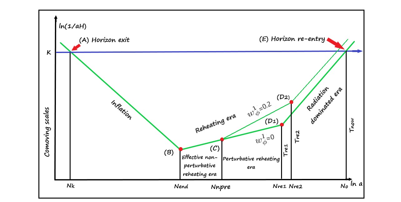
The standard and well-studied mechanism to consider the non-perturbative effect during reheating is called preheating. This stage is essentially the combination of a highly non-linear process of parametric resonance and subsequent thermalization. The well-known fact that generically non-perturbative preheating mechanism does not completely decay inflaton into the radiation field. Therefore, subsequent perturbative decay will be necessary to complete the reheating process. To the best of our knowledge, the reference Maity:2018dgy has considered this issue for the first time and studied perturbative reheating, followed by the preheating considering a specific model of chaotic type inflation. However, generically the preheating mechanism is model dependent. Hence, combining the end of preheating and subsequent model-independent perturbative reheating is somewhat irreconcilable. Therefore, our objective in the following sections would be to make these two phases reconcilable.

Instead of dwelling into explicit non-perturbative computation during the preheating stage, we will adopt an effective model-independent approach following the reference martin. The basic idea is to assume the dynamics of preheating to be solely governed by an effective equation of state $\omega_{eff}$ supplemented with the total energy conservation law in terms of its constituents. As already emphasized in the introduction, the information about the actual non-perturbative dynamic will be encoded though considering its universal features into our effective dynamics.

As has been pointed out already, during the non-perturbative dynamics, inflaton decay is not complete, and typically it is around $50\%$ of its total comoving energy, which is being transferred into the daughter fields. Furthermore, inflation models with quadratic potential near the minimum, the non-perturbative reheating does not lead to the equation of state, $\omega=\frac{1}{3}$, which is expected at the end point of reheating Podolsky:2005bw; Maity:2018qhi. Our essential idea would be to correctly utilize those results as the end point conditions of our proposed effective dynamics in place of preheating. After the end of this, the usual Boltzmann perturbative reheating process will follow. The second phase completes the reheating process by leading to the correct state equation with relativistic degrees of freedom as the dominant components collectively called radiation. The Fig.2 illustrates our methodology of calculation. Throughout this paper, we call this as two-phase reheating process.
phase-I:(Effective non-perturbative phase) During the early stage of reheating, the phase will be described by total energy density $\rho_{T}=\rho_{R}+\rho_{\phi}$ and the constant effective equation state $w_{eff}$. Hence the evolution will be described by,

$\displaystyle\rho_{T}=\rho_{Te}\left(\frac{a_{end}}{a}\right)^{3(1+w_{eff})}~,$

(35)

where $\rho_{Te}$ is the total energy density at the end of the inflation. $a_{end}$ is the scale factor at the end of the inflation. In this section we will build up our formalism considering two matter component with $\rho_{\phi}$, $\rho_{R}$ as the inflaton energy density and radiation energy density respectively at any instant of time. In the subsequent section we will add dark matter as a third component as an extension. Nonetheless, from the total energy expression one can write down the following equation follows from Eq.35,

$\displaystyle\dot{\rho_{\phi}}+\dot{\rho_{R}}+3H(1+w_{eff})(\rho_{\phi}+\rho_{R})=0~.$

(36)

To reduce the number of unknown parameters, to this end we will also utilize total energy conservation relation considering individual equation of state of the inflaton $(\omega_{\phi})$ and the radiation field $(\omega_{R}=1/3)$ described as

$\displaystyle\dot{\rho_{\phi}}+3H(1+w_{\phi})\rho_{\phi}+\dot{\rho_{R}}+4H\rho_{R}=0~.$

(37)

Given the aforementioned constraint relation one obtains the possible restricted value of the effective equation of state, $\omega_{eff}$. To find those restrictions we combine above two eqs.(36) and (37), and obtain the following consistency relation,

$\displaystyle\frac{\rho_{R}}{\rho_{\phi}+\rho_{R}}=\frac{3\left(w_{\phi}-w_{eff}\right)}{3w_{\phi}-1}~.$

(38)

Right at the end of inflation or the beginning of the preheating phase, the energy density of the radiation part will naturally be closed to zero $\rho_{R}\simeq 0$. As time evolves, $\rho_{R}$ increases due to decaying inflaton. This initial condition automatically restricts the possible values of $w_{eff}$ to be very closed to that of the inflaton equation of state $w_{\phi}$. Of course more appropriate approach would be to assume the inflaton equation of state evolving from the value very closed to $\omega_{\phi}$ to the value required in the next phase. We will comment on this issue at the appropriate place during our discussion. However, from the usual numerical lattice simulation, the preheating phase’s significant duration is dominated by the inflaton. Hence, the equation of state will naturally be closed to that of the inflaton field. Thus, our effective dynamics approach towards preheating truly captures all these necessary properties of the non-perturbative dynamics. As $w_{eff}$ turned out to be no longer a free parameter and constrained by the above consistency relation (38), our following analysis will be based on this important result. Throughout our study we consider models for which the inflaton equation of state during phase-I $\omega_{\phi}=0$, and consequently following Eq.38 we choose two values of effective equation of state $\omega_{eff}=(10^{-6},10^{-3}$). This choice will automatically fixes the initial radiation densities during phase-I as $\rho_{R}/(\rho_{\phi}+\rho_{R})=(3\times 10^{-6},3\times 10^{-3})$. We will see the maximum reheating temperature crucially depends upon these initial conditions.

Phase-II: (Perturbative phase) Once the preheating dynamics ends the usual Boltzmann perturbative reheating follows. During this period various components of the total energy density satisfy the following standard Boltzmann equations Riotto,

$$\dot{\rho}_{\phi}+3H(1+w_{\phi}^{1})\rho_{\phi}+\Gamma_{\phi}\rho_{\phi}(1+w_{\phi}^{1})=0~,$$

(39)

$$\dot{\rho}_{R}+4H\rho_{R}-\Gamma_{\phi}\rho_{\phi}(1+w_{\phi}^{1})=0~,$$

(40)

where the inflaton field $\phi$ decays into radiation with the decay rate $\Gamma_{\phi}$. $\omega_{\phi}^{1}$ represents inflaton equation of state during perturbative reheating. Important to note that inflaton equation of state during phase-I, $\omega_{\phi}$ is taken to be different than that of the phase-II, $\omega_{\phi}$. This is where we will again consider lattice simulation results as another important input.

Now that we have identified the full reheating phase in terms of two distinct stages, we will numerically solve all those equations self consistently. With the appropriate dimensionless rescaled variables for the inflaton and radiation energy densities,

$$\varPhi=\frac{\rho_{\phi}a^{3(1+w_{\phi})}}{m_{\phi}^{(1-3w_{\phi})}}~;~R(t)=\rho_{R}a^{4}~~,$$

(41)

governing equations for the effective dynamical preheating phase turn into the following form,

$\displaystyle\left.\begin{array}[]{c}\frac{\varPhi^{\prime}}{A^{3w_{\phi}}}+\frac{R^{\prime}}{A}=0~,\\ \frac{\varPhi^{\prime}}{A^{2+3w_{\phi}}}+\frac{R}{A^{4}}[3(1+w_{eff})-4]+\frac{R^{\prime}}{A^{3}}+\frac{3\varPhi(w_{eff}-w_{\phi})}{A^{3(1+w_{\phi})}}=0\end{array}\right\},~~\mbox{\bf Phase I}$

and the associated governing equations for the subsequent perturbative phase will reduce into

$\displaystyle\left.\begin{array}[]{c}\varPhi^{{}^{\prime}}+C_{1}(1+w_{\phi}^{1})\frac{A^{1/2}\varPhi}{X}=0~,\\ R^{{}^{\prime}}-C_{1}(1+w_{\phi}^{1})\frac{A^{\frac{3(1-2w_{\phi}^{1})}{2}}\varPhi}{X}=0\end{array}\right\}.~~~~~~~\mbox{\bf Phase-II}$

The rescaled scale factor is defined as $A=\frac{a}{a_{end}}$. ”Prime”(^′) represents derivative with respect to A. The constant $C_{1}$ and redefined variables are,

$$X=\frac{\varPhi}{A^{3w_{\phi}^{1}}}+\frac{R}{A}~;~C_{1}=\frac{\sqrt{3}M_{p}\varGamma_{\phi}}{m_{\phi}^{2}}~.$$

(48)

$m_{\phi}$ is the mass of the inflaton. In next section we will describe the methodology for solving the above set of equations numerically.

Let us describe the strategy of our numerical study. We first identify the inflation model-dependent input parameters as $N_{k},H_{k},V_{end}$ for a particular CMB scale $k$. For a given a canonical inflaton potential $V(\phi)$, the inflationary e-folding number $N_{k}$ and Hubble constant $H_{k}$ can be expressed as

$\displaystyle N_{k}=\log\left(\frac{a_{end}}{a_{k}}\right)=\int_{\phi_{end}}^{\phi_{k}}\frac{3}{2}\frac{V(\phi)}{V^{\prime}(\phi)}d\phi=\int_{\phi_{k}}^{\phi_{end}}\frac{|d\phi|}{\sqrt{2\epsilon_{v}}M_{p}}~~,~~H_{k}=\frac{1}{3M_{p}^{2}}V(\phi_{k})=\frac{\pi M_{p}\sqrt{r_{k}A_{s}}}{\sqrt{2}}~,$

(49)

where, the field values at a particular scale $k$, $(\phi_{end},\phi_{k})$ are computed form the condition of end of inflation,

$\displaystyle\epsilon(\phi_{end})=\frac{1}{2M_{p}^{2}}\left(\frac{V^{\prime}(\phi_{end})}{V(\phi_{end})}\right)^{2}=1,$

(50)

and equating a particular value of scalar spectral index with $n_{s}(\phi_{k})$. Therefore, we will get explicit relations between $(N_{k},n_{s}^{k})$ and $(H_{k},n_{s}^{k})$. The well known inflationary input parameters can be found out from the following equations

$$n_{s}^{k}=1-6\epsilon(\phi_{k})+2\eta(\phi_{k})~,~r_{k}=16\epsilon(\phi_{k})~~,$$

(51)

which are expressed in terms of slow-roll parameters

$$\epsilon_{v}=\frac{M_{p}^{2}}{2}\left(\frac{V^{\prime}}{V}\right)^{2}~~;~~|\eta_{v}|=M_{p}^{2}\frac{|V^{\prime\prime}|}{V}~.$$

(52)

The reheating parameters $N_{re},T_{rad}$ will implicitly depend upon the scalar spectral index $n_{s}^{k}$ for a given scale. The above expression can be inverted to find $\phi_{k}$ in terms of the scalar spectral index. After identifying all required parameters from inflation, we will set the initial conditions for subsequent reheating dynamics. Using all these relations among those parameters, one can establish the connection between CMB anisotropy and reheating through inflation.

Phase-I initial condition: The initial conditions for phase-I of the reheating dynamics (effective non-perturbative era) are set by the end of inflation at $A=1$ and the equation 38. Those are as follows,

$$\varPhi(A=1)=\frac{3}{2}\frac{V_{end}(\phi)}{m_{\phi}^{4}}~~;~~R(A=1)=\frac{3\left(\omega_{eff}-\omega_{\phi}\right)}{1-3\omega_{eff}}~\varPhi(A=1)~.$$

(53)

Where $V_{end}(\phi)$ which is defined at the end of inflation, fixed by $\phi_{end}$. The initial Hubble expansion rate is expressed as $H_{I}$= ${\rho_{\phi}^{end}}/{3M_{p}^{2}}$.

Subsequent perturbative dynamics will now crucially depend on the end point of the first phase of reheating namely the phase-I. On this issue we rely on the actual non-perturbative lattice simulation results Podolsky:2005bw; Figueroa:2016wxr; Maity:2018qhi considering specific model of reheating where the inflaton field is assumed to couple with the reheating field. This system has been studied quite extensively Allahverdi:2010xz; Amin:2014eta in the literature by using the publicly available numerical package LATTICEEASYFelder:2000hq and its parallelized version CLUSTEREASYFelder:2007nz. The non-perturbative analysis for different inflationary models has been proved to yield some universal results which will be our important input for the numerical analysis. Extensive works on non-perturbative reheating analysis yields an important fact that only the $50\%$ of the total comoving inflaton energy density is getting transferred into the daughter field. Additionally the inflaton equation of state tends to achieve a steady state value depending upon the power law form of the inflaton potential near its minimum. For example if one assumes the inflaton potential to be of power law form $V\sim\phi^{n}$, for chaotic type model namely $n=2$, non-perturbative phase ends with steady value of the equation of state $\sim 0.2$. However, for other value of $n\geq 4$, the equation of state approaches $\omega=\frac{1}{3}$ at the end point of the non-perturbative reheating. These are the crucial quantitative results from non-perturbative preheating dynamics we will be utilizing in our analysis for the phase-II dynamcis.

Phase-II initial condition: After the phase-I dynamics, the pertubative dynamics will automatically follow. However, important point would be to identify the appropriate boundary conditions. The starting moment of phase-II will be set by the normalized scale factor $A_{npre}={a_{npre}}/{a_{end}}$ which is the ratio between the scale factor at the end of the effective non-perturbative epoch namely phase-I $a_{npre}$, and the end of the inflation. The initial conditions for the dimensionless comoving densities are

$\displaystyle\varPhi=\varPhi(A_{npre})~~;~~\frac{R(A_{npre})}{R(A_{npre})+\varPhi(A_{npre})}\simeq\frac{1}{2}.$

(54)

It is important to realize that the initial condition is determined by $50\%$ decay of the total comoving energy density $\rho_{T}$. Further, we have numerically checked that our results do not seem to depend both qualitatively as well as quantitatively much on the amount of decay within $40\%-60\%$ of the total energy at the end of phase-I. For the analysis, we further assume the inflaton equation of state $\omega_{\phi}^{1}\simeq 0.2$ irrespective of the models under consideration. This approximate value is again another important input from the Lattice simulation. For comparison, we also consider the cases where either phase-I or phase-II evolution completely governs the reheating dynamics.

Determining the reheating parameters: Once we numerically solve the reheating dynamics, we define one of the important parameters called reheating temperature $T_{re}$, which is generically identified as the radiation temperature $T_{rad}$ when the condition $H(t)=\Gamma_{\phi}$ is satisfied,

$\displaystyle H(A_{re})^{2}=\left(\frac{\dot{A}_{re}}{A_{re}}\right)^{2}=\frac{\rho_{\phi}(\Gamma_{\phi},A_{re},n_{s}^{k})+\rho_{R}(\Gamma_{\phi},A_{re},n_{s}^{k}))}{3M_{p}^{2}}=\Gamma_{\phi}^{2}~,$

(55)

where $A_{re}$ is the normalized scale factor at the end of the reheating. Accordingly, the reheating temperature in terms of radiation temperature ($T_{rad}$) is expressed as,

$\displaystyle T_{re}=T_{rad}^{end}=\left(\frac{30}{\pi^{2}g_{*}(T)}\right)^{1/4}\rho_{R}(\Gamma_{\phi},A_{re},n_{s}^{k})^{1/4}~.$

(56)

Furthermore, the e-folding number during reheating $N_{re}$ consists of two contributions born out of two distinct phases as

$$N_{re}=\log\left(\frac{a_{re}}{a_{end}}\right)=\log\left(\frac{a_{re}}{a_{npre}}\frac{a_{npre}}{a_{end}}\right)=N_{pre}+N_{npre}~,$$

(57)

$\displaystyle N_{pre}=\log\left(\frac{a_{re}}{a_{npre}}\right)~~;~~N_{npre}=\log\left(\frac{a_{npre}}{a_{end}}\right)~,$

(58)

where $N_{pre}$ and $N_{npre}$ are the e-folding number during perturbative and effective nonperturbative region respectively. Combining equations (8) and (57), we obtain the most important modification of Eq.8 relating the reheating and inflationary parameters,

$\displaystyle T_{re}=\left(\frac{43}{11g_{re}}\right)^{1/3}\left(\frac{a_{0}T_{0}}{k}\right)H_{k}e^{-N_{k}}e^{-N_{npre}}e^{-N_{pre}}~.$

(59)

Now connecting equations (55), (56) and (59), we can establish one to one correspondence between $T_{re}$ and $\Gamma_{\phi}$.

As described before, we will consider three possible cases and compare the results

$\displaystyle\begin{array}[]{ccc}\mbox{Case-I}&N_{npre}\neq 0~,~N_{pre}\neq 0&~~\mbox{Phase-I + Phase-II}\\ \mbox{Case-II}&N_{npre}\neq 0~~;~~N_{pre}=0&~~\mbox{Kamionkawski et al 2014 \cite[cite]{\@@bibref{Authors Phrase1YearPhrase2}{martin}{\@@citephrase{(}}{\@@citephrase{)}}}}\\ \mbox{Case-III}&N_{npre}=0~~;~~N_{pre}\neq 0&~~\mbox{Phase-II, Discussed in the previous section}\end{array}$

To this end let us specifically mention about the case-II, when perturbative dynamics ceases to exist. This particular procedure proposed in martin, has been studied quite extensively in the literature reheating. In this particular phase, dynamics is solely governed by the effective equation of state $\omega_{eff}$. The explicit decay of inflaton does not appear in the computation. However, information about the decay constant $\Gamma_{\phi}$ is extracted from the equilibrium condition $\Gamma_{\phi}=H$, where the reheating temperature ($T_{re}$) is defined as $T_{re}=0.2\left(\frac{200}{g_{*}}\right)^{1/4}\left(\Gamma_{\phi}M_{pl}\right)^{1/2}$, with $g_{*}$ being the effective number of relativistic degrees of freedom. However, not to ignore an important difference between the phase-I described before and the approach devised in martin or case-II for the present study is the additional conservation equation 38. This essentially differentiates the regime of applicability of these two approaches. Phase-I dynamics is assumed to be applicable in the early non-perturbative regime. Whereas, since condition 38 does not exist, the original Kamionkowski et almartin approach is effectively applicable throughout the full period of reheating without any microscopic details. Further, the value of $\omega_{eff}$ is no longer constrained to be very closed to the inflaton equation of state during phase-I. This relation essentially helps us to compare the results for various scenarios we consider. To avoid symbol confusion whenever we study case-II, we use the symbol $\omega_{eff}^{K}$ instead $\omega_{eff}$ which we reserve for two-phase reheating dynamics.

Before moving on to a particular model, let us analytically estimate the maximum reheating temperature and its dependence upon the initial condition following the same line as before. Considering the standard definition of the radiation temperature $T_{rad}=\left(\frac{30}{\pi^{2}g_{*}}\rho_{R}\right)^{1/4}$, and computing the radiation energy density during phase II following the Eqs.(39), (40), (36) and (37) the approximate radiation temperature assumes the following form (see appendix A for details calculation)

$\displaystyle T_{rad}=\left(\frac{\rho_{\phi}^{in}\Gamma_{\phi}(1+\omega_{\phi}^{1})}{\beta x^{4}H_{in}}\left[\frac{2}{5-c}\left(x^{\frac{5-c}{2}}-1\right)+\frac{\rho_{R}^{in}}{\rho_{\phi}^{in}}\left(\frac{1-x^{\frac{c+3}{2}}}{c+3}+\frac{H_{in}}{\Gamma_{\phi}(1+\omega_{\phi}^{1})}\right)\right]\right)^{1/4}~~,$

(64)

where $x$, $\beta$, $c$ and $H_{in}$ express as

$\displaystyle x=\frac{a}{a_{npre}}~,~\beta=\frac{\pi^{2}g_{*}(T)}{30}~,~c=3\omega_{\phi}^{1}~,~H_{in}=\frac{\sqrt{\rho_{\phi}^{in}}}{\sqrt{3}M_{P}}~~.$

(65)

In the above expression $\rho_{\phi}^{in}$, $\rho_{R}^{in}$ represent inflaton and radiation energy density respectively at the end of phase-I or the beginning of phase-II

$\displaystyle\rho_{\phi}^{in}=\rho_{\phi}(a=a_{npre})~,~\rho_{R}^{in}=\rho_{R}(a=a_{npre})~~.$

(66)

The maximum radiation temperature defined at the point $x_{max}=a_{max}/a_{npre}$, where $\frac{dT_{rad}}{dx}=0$, which gives us the maximum radiation temperature for two phase reheating expressed in terms of dimensionless comoving densities,

$\displaystyle T_{rad}^{max}\simeq D^{1/4}\left[1+\frac{(3+c)R(A_{npre})}{8\Phi(A_{npre})A_{npre}^{1-c}}\left(\frac{1-x_{max,p}^{\frac{c+3}{2}}}{c+3}+\frac{\sqrt{\Phi(A_{npre})A_{npre}^{-3(1+\omega_{\phi}^{1})}m_{\phi}^{4}}}{\sqrt{3}M_{p}\Gamma_{\phi}(1+\omega_{\phi}^{1})}\right)\right]~~$

(67)

$\displaystyle D=\left(\frac{2\Gamma_{\phi}\sqrt{3M_{p}^{2}\Phi(A_{npre})A_{npre}^{-3(1+\omega_{\phi}^{1})}m_{\phi}^{4}}}{\left(3+c\right)\beta x_{max,p}^{4}}\right)^{1/4}~~,~x_{max,p}=\left(\frac{8}{3+c}\right)^{\frac{2}{5-c}}~~.$

(68)

One particularly notices the correction term in the maximum radiation temperature due to initial comoving radiation density $R(A_{npre})$ at the beginning of phase-II. It boils down to well know expression $T_{re}^{max}=D^{1/4}$ in the $R(A_{npre})=0$ limit same as Eq.17. In this above expression, we ignored the contribution of dark matter. However, generically during the reheating period, dark matter is not the dominant component, therefore, the numerical value of the reheating temperature will not be affected. The analytic expression for the dimensionless comoving density during phase II related to the density at the end of inflation will be

$\displaystyle\Phi(A_{npre})=\left(1-3\omega_{eff}\right)\Phi(A=1)A_{npre}^{-3\omega_{eff}}~~.$

(69)

Where $A_{npre}$ is the normalized scale factor at the end of the effective dynamics (phase I)

$\displaystyle A_{npre}=\frac{1-3\omega_{eff}}{3\omega_{eff}}~~.$

(70)

One of our important results from the above expression for the maximum reheating temperature is the highest radiation temperature, which is defined at $T_{rad}^{max}=T_{re}^{max}$ corresponding to a given $n_{s}^{max}$. As we change the value of $\omega_{eff}=(10^{-3}\rightarrow 10^{-6}$), the maximum reheating temperature changes as $T_{re}^{max}=(10^{13}\to 10^{10})$ GeV. Once we set $R(A_{npre})=0$, the maximum reheating temperature becomes $T_{re}^{max}\sim 10^{15}$ GeV as expected (see Eqs.17,18). Proceeding further, we can also obtain the approximation expression for the reheating temperature itself. Utilizing the expression of Hubble constant at the equilibrium point ($H_{re}=\Gamma_{\phi}$), and subsequent entropy conservation, one arrives at the following expression

$\displaystyle T_{re}^{4}\simeq\frac{x_{re}^{4}\rho_{\phi}^{in}}{3\beta M_{p}^{2}}\left[\frac{G^{4}\beta}{\rho_{\phi}^{in}}+\frac{5-c}{2\left(c+3\right)}\frac{\rho_{R}^{in}}{\rho_{\phi}^{in}}\left(\frac{G^{4}\beta}{\rho_{\phi}^{in}}-\frac{\rho_{R}^{in}}{\rho_{\phi}^{in}}\right)x_{re}^{c-1}\right]~~.$

(71)

Where, $x_{re}=a_{re}/a_{npre}$ can be recognize as

$\displaystyle x_{re}=\left(\frac{\alpha}{\eta}\right)^{\frac{1}{c-1}}~~,$

(72)

Here

$\displaystyle\alpha=\frac{G^{4}\beta}{\rho_{\phi}^{in}}~,~\eta=\frac{5-c}{2}\left(\frac{G^{4}\beta}{\rho_{\phi}^{in}}-\frac{\rho_{R}^{in}}{\rho_{\phi}^{in}}\right)\left[\frac{\rho_{R}^{in}}{\left(c+3\right)\rho_{\phi}^{in}}+\frac{5-c}{2}\frac{3M_{p}^{2}H_{in}^{2}}{\rho_{\phi}^{in}\left(1+\omega_{\phi}^{1}\right)^{2}}\left(\frac{G^{4}\beta}{\rho_{\phi}^{in}}-\frac{\rho_{R}^{in}}{\rho_{\phi}^{in}}\right)\right]~.$

(73)

The detailed derivation of all the aforementioned equations for the reheating temperature in the appendix B. Now we will consider a class of inflationary models of inflation and analyze our proposal of two-phase reheating scenario.

References

- (1) A. H. Guth, Phys.Rev. D 23, 347356 (1981); A. D. Linde, Phys. Lett. B 108, 389393 (1982); A. Albrecht and P. J. Steinhardt, Phys. Rev. Lett. 48, 12201223 (1982); A. A. Starobinsky, Adv. Ser. Astrophys. Cosmol. 3, 130-133 (1987)
- (2) Y. Akrami et al. [Planck Collaboration], arXiv:1807.06211 [astro-ph.CO].
- (3) A. R. Liddle and D. H. Lyth, “Cosmological inflation and large scale structure,”, Cambridge University Press, (2000)
- (4) A. Berera, Phys. Rev. Lett. 75, 3218-3221 (1995) doi:10.1103/PhysRevLett.75.3218 [arXiv:astro-ph/9509049 [astro-ph]].
- (5) A. Berera, Phys. Rev. D 55, 3346-3357 (1997) doi:10.1103/PhysRevD.55.3346 [arXiv:hep-ph/9612239 [hep-ph]].
- (6) J. Martin and C. Ringeval, Phys. Rev. D82, 023511 (2010); J. Martin, C. Ringeval and V. Vennin, Phys. Rev.Lett. 114, 081302 (2015); L. Dai, M. Kamionkowski and J. Wang, Phys. Rev. Lett. 113, 041302 (2014).
- (7) M. Drewes, JCAP 1603 (2016), 013 [arXiv:1511.03280 [astro-ph.CO]].
- (8) I. Dalianis and Y. Watanabe, JHEP 02, 118 (2018) [arXiv:1801.05736 [hep-ph]].
- (9) M. Drewes, [arXiv:1903.09599 [astro-ph.CO]].
- (10) E. W. Kolb, A. D. Linde and A. Riotto, Phys. Rev. Lett. 77, 4290-4293 (1996) [arXiv:hep-ph/9606260 [hep-ph]].
- (11) A. Dolgov, K. Freese, R. Rangarajan and M. Srednicki, Phys. Rev. D 56, 6155-6165 (1997) [arXiv:hep-ph/9610405 [hep-ph]].
- (12) A. Riotto and M. Trodden, Ann. Rev. Nucl. Part. Sci. 49, 35-75 (1999) [arXiv:hep-ph/9901362 [hep-ph]].
- (13) J. Garcia-Bellido, D. Y. Grigoriev, A. Kusenko and M. E. Shaposhnikov, Phys. Rev. D 60, 123504 (1999) [arXiv:hep-ph/9902449 [hep-ph]].
- (14) R. Allahverdi, B. A. Campbell and J. R. Ellis, Nucl. Phys. B 579, 355-375 (2000) [arXiv:hep-ph/0001122 [hep-ph]].
- (15) S. Davidson, M. Losada and A. Riotto, Phys. Rev. Lett. 84, 4284-4287 (2000) [arXiv:hep-ph/0001301 [hep-ph]].
- (16) A. Megevand, Phys. Rev. D 64, 027303 (2001) [arXiv:hep-ph/0011019 [hep-ph]].
- (17) S. A. Gorbunov et al. [NEWSdm], Phys. Atom. Nucl. 83, no.1, 83-91 (2020)
- (18) M. S. Turner and F. Wilczek, Phys. Rev. Lett. 65, 3080-3083 (1990)
- (19) A. Kosowsky, M. S. Turner and R. Watkins, Phys. Rev. Lett. 69, 2026-2029 (1992)
- (20) F. Finelli and R. H. Brandenberger, Phys. Rev. Lett. 82, 1362-1365 (1999) [arXiv:hep-ph/9809490 [hep-ph]].
- (21) R. Easther, J. T. Giblin, Jr. and E. A. Lim, Phys. Rev. Lett. 99, 221301 (2007) [arXiv:astro-ph/0612294 [astro-ph]].
- (22) R. Easther and E. A. Lim, JCAP 04, 010 (2006) [arXiv:astro-ph/0601617 [astro-ph]].
- (23) J. Garcia-Bellido and D. G. Figueroa, Phys. Rev. Lett. 98, 061302 (2007) [arXiv:astro-ph/0701014 [astro-ph]].
- (24) J. Garcia-Bellido, D. G. Figueroa and A. Sastre, Phys. Rev. D 77, 043517 (2008) [arXiv:0707.0839 [hep-ph]].
- (25) J. F. Dufaux, A. Bergman, G. N. Felder, L. Kofman and J. Uzan, Phys. Rev. D 76, 123517 (2007) [arXiv:0707.0875 [astro-ph]].
- (26) N. Bernal and F. Hajkarim, Phys. Rev. D 100, 063502 (2019) [arXiv:1905.10410 [astro-ph.CO]].
- (27) K. D. Lozanov and M. A. Amin, Phys. Rev. D 99, no.12, 123504 (2019) [arXiv:1902.06736 [astro-ph.CO]].
- (28) P. Saha, S. Anand and L. Sriramkumar, [arXiv:2005.01874 [astro-ph.CO]].
- (29) D. Maity and P. Saha, Phys. Rev. D 98, no.10, 103525 (2018) [arXiv:1801.03059 [hep-ph]].
- (30) D. Maity and P. Saha, Phys. Dark Univ. 25, 100317 (2019) [arXiv:1804.10115 [hep-ph]].
- (31) D. Maity and P. Saha, JCAP 07, 018 (2019) [arXiv:1811.11173 [astro-ph.CO]].
- (32) L. Kofman, A. D. Linde and A. A. Starobinsky, Phys. Rev. Lett. 73, 3195 (1994); L. Kofman, A. D. Linde and A. A. Starobinsky, Phys. Rev. D 56, 3258 (1997); ; Y. Shtanov, J. H. Traschen and R. H. Brandenberger, Phys. Rev. D 51 (1995) 5438.
- (33) K. Freese, E. I. Sfakianakis, P. Stengel and L. Visinelli, JCAP 05, 067 (2018) [arXiv:1712.03791 [hep-ph]].
- (34) R. Easther, R. Flauger and J. B. Gilmore, JCAP 04, 027 (2011) doi:[arXiv:1003.3011 [astro-ph.CO]].
- (35) D. G. Figueroa and F. Torrenti, JCAP 1702, no. 02, 001 (2017) [arXiv:1609.05197 [astro-ph.CO]].
- (36) S. Antusch, D. G. Figueroa, K. Marschall and F. Torrenti, [arXiv:2005.07563 [astro-ph.CO]].
- (37) K. D. Lozanov and M. A. Amin, Phys. Rev. Lett. 119, no. 6, 061301 (2017) [arXiv:1608.01213 [astro-ph.CO]].
- (38) K. D. Lozanov and M. A. Amin, Phys. Rev. D 97 (2018) no.2, 023533 [arXiv:1710.06851 [astro-ph.CO]].
- (39) P. Adshead, R. Easther, J. Pritchard and A. Loeb, JCAP 1102, 021 (2011); R. Easther and H. V. Peiris, Phys. Rev. D85, 103533 (2012); J. B. Munoz and M. Kamionkowski, Phys. Rev. D91, 043521 (2015); J. L. Cook, E. Dimastrogiovanni, D. A. Easson and L. M. Krauss, JCAP 1504, 047 (2015).
- (40) C. Patrignani et al. [Particle Data Group], Chin. Phys. C 40, no. 10, 100001 (2016).
- (41) J. Ellis etal, JCAP 1507, 050 (2015).
- (42) M. Drewes, J. U. Kang and U. R. Mun, JHEP 1711 (2017) 072 [arXiv:1708.01197 [astro-ph.CO]].
- (43) M.Yu.Khlopov, A.D.Linde, Phys. Lett. 138B, 265, (1984); V. Domcke and J. Heisig, Phys. Rev. D92, 103515 (2015)
- (44) Planck Collaboration: P. A. R. Ade et al., 594, A20 (2016); Keck Array, BICEP2 Collaborations: P. A. R. Ade et al., Phys. Rev. Lett. 116, 031302 (2016).
- (45) Euclid Theory Working Group Collaboration, L. Amendola et al., Living. Rev.Rel. 16, 6 (2013).
- (46) PRISM Collaboration, P. Andre et al., [arXiv:1306.2259].
- (47) G. F. Giudice, E. W. Kolb, and A. Riotto, Phys. Rev. D64, 023508 (2001).
- (48) A. D. Linde, Phys. Lett. 129B, 177 (1983).
- (49) K. Freese, J. A. Frieman and A. V. Olinto, Phys. Rev. Lett. 65, 3233 (1990).
- (50) A. A. Starobinsky, Phys. Lett. B 91, 99 (1980).
- (51) F. L. Bezrukov and M. Shaposhnikov, Phys.Lett. B 659, 703 (2008).
- (52) R. Kallosh and A. Linde, JCAP 1307, 002 (2013); R. Kallosh, A. Linde and D. Roest, JHEP 1311, 198 (2013).
- (53) L. F. Abbott, E. Farhi and M. B. Wise, Phys. Lett. 117B (1982) 29. A. Albrecht, P. J. Steinhardt, M. S. Turner and F. Wilczek, Phys. Rev. Lett. 48 (1982) 1437.
- (54) M. E. Peskin and D. V. Schroeder, An Introduction to quantum field theory,
- (55) J. Garcia-Bellido, D. G. Figueroa and J. Rubio, Phys. Rev. D 79 (2009) 063531 [arXiv:0812.4624 [hep-ph]].
- (56) P. B. Greene and L. Kofman, Phys. Lett. B 448 (1999) 6-12. [hep-ph/9807339].
- (57) D. Maity and P. Saha, Class. Quant. Grav. 36, 045010 (2019) [arXiv:1902.01895 [gr-qc]].
- (58) Planck Collaboration: P.A.R. Ade et al. Astron.Astrophys. 571, A22 (2014); ibid Astron.Astrophys. 594, A20 (2016).
- (59) M. A. Amin, M. P. Hertzberg, D. I. Kaiser and J. Karouby Int. J. Mod. Phys. 24 (2014) 1530003 [arXiv:1410.3808 [hep-ph]].
- (60) A.D Linde Lect.Notes Phys.738 (2008) 1 [arXiv:0705.0164 [hep-th]].
- (61) B. A. Bassett, S. Tsujikawa and D. Wands Mod.Phys.78 (2006) 537 [astro-ph/0507632]
- (62) Daniel J. H. Chung, Edward W. Kolb, Antonio Riotto, Phys.Rev.D 60, 063504 (1999)
- (63) D. I. Podolsky, G. N. Felder, L. Kofman and M. Peloso, Phys. Rev. D 73, 023501 (2006)
- (64) D. Maity, Nucl. Phys. B 919, 560 (2017) [arXiv:1606.08179 [hep-ph]].
- (65) E. Komatsu et al. [WMAP Collaboration], Astrophys. J. Suppl. 192, 18 (2011) [arXiv:1001.4538 [astro-ph.CO]].
- (66) R. Allahverdi, R. Brandenberger, F. Cyr-Racine and A. Mazumdar, Ann. Rev. Nucl. Part. Sci. 60, 27-51 (2010) [arXiv:1001.2600 [hep-th]].
- (67) M. A. Amin, M. P. Hertzberg, D. I. Kaiser and J. Karouby, Int. J. Mod. Phys. D 24, 1530003 (2014) [arXiv:1410.3808 [hep-ph]].
- (68) G. N. Felder and I. Tkachev, Comput. Phys. Commun. 178, 929 (2008) [hep-ph/0011159].
- (69) G. N. Felder, Comput. Phys. Commun. 179, 604 (2008) [arXiv:0712.0813 [hep-ph]].
- (70) G. F. Giudice, E. W. Kolb and A. Riotto, Phys. Rev. D 64, 023508 (2001) [hep-ph/0005123].
- (71) F. L. Bezrukov and M. Shaposhnikov, Phys. Lett. B 659, 703 (2008) [arXiv:0710.3755 [hep-th]].
- (72) A. A. Starobinsky, Phys. Lett. 91B, 99 (1980) [Adv. Ser. Astrophys. Cosmol. 3, 130 (1987)].
- (73) K. Griest and M. Kamionkowski, Phys. Rev. Lett. 64, 615 (1990).
- (74) M. Kawasaki, K. Kohri and N. Sugiyama, Phys. Rev. Lett. 82, 4168 (1999) [astro-ph/9811437].
- (75) M. Kawasaki, K. Kohri and N. Sugiyama, Phys. Rev. D 62, 023506 (2000) [astro-ph/0002127].
- (76) G. Steigman, Ann. Rev. Nucl. Part. Sci. 57, 463 (2007) [arXiv:0712.1100 [astro-ph]].
- (77) B. D. Fields, P. Molaro and S. Sarkar, Chin. Phys. C 38, 339 (2014) [arXiv:1412.1408 [astro-ph.CO]].
- (78) M. Gerbino, K. Freese, S. Vagnozzi, M. Lattanzi, O. Mena, E. Giusarma and S. Ho, Phys. Rev. D 95, 043512 (2017) [arXiv:1610.08830 [astro-ph.CO]].
- (79) K. Freese and W. H. Kinney, JCAP 1503, 044 (2015) [arXiv:1403.5277 [astro-ph.CO]].
- (80) W. T. Emond, P. Millington and P. M. Saffin, JCAP 1809, 041 (2018) [arXiv:1807.11726 [hep-th]].
- (81) V. C. Rubin, Hautes Energies en Astrophysique: Proceedings, Ecole d’Et de Physique Thorique, Les Houches, France, 1966, vol. 1, pp. 133-152, 1967.
- (82) V. C. Rubin and W. Ford, Jr., Astrophys. J. 159, 379-403 (1970)
- (83) W. Hu and S. Dodelson, Ann. Rev. Astron. Astrophys. 40, 171 (2002) [arXiv:astro-ph/0110414 [astro-ph]].
- (84) G. Bertone, D. Hooper and J. Silk, Phys. Rept. 405, 279 (2005) [arXiv:hep-ph/0404175 [hep-ph]].
- (85) N. Jarosik et al. [WMAP], Astrophys. J. Suppl. 192, 14 (2011) [arXiv:1001.4744 [astro-ph.CO]].
- (86) N. Aghanim et al. [Planck], [arXiv:1807.06209 [astro-ph.CO]]. Cite Article
- (87) T. Tenkanen, JHEP 09, 049 (2016) [arXiv:1607.01379 [hep-ph]].
- (88) M. Heikinheimo, T. Tenkanen, K. Tuominen and V. Vaskonen, PoS ICHEP2016, 825 (2016) [arXiv:1611.04951 [astro-ph.CO]].
- (89) N. Bernal, M. Heikinheimo, T. Tenkanen, K. Tuominen and V. Vaskonen, Int. J. Mod. Phys. A 32, (2017) [arXiv:1706.07442 [hep-ph]].
- (90) L. J. Hall, K. Jedamzik, J. March-Russell and S. M. West, JHEP 03, 080 (2010) [arXiv:0911.1120 [hep-ph]].
- (91) Y. Mambrini, K. A. Olive, J. Quevillon and B. Zaldivar, Phys. Rev. Lett. 110, (2013) [arXiv:1302.4438 [hep-ph]].
- (92) X. Chu, Y. Mambrini, J. Quevillon and B. Zaldivar, JCAP 01, 034 (2014) [arXiv:1306.4677 [hep-ph]].
- (93) M. Blennow, E. Fernandez-Martinez and B. Zaldivar, JCAP 01, 003 (2014) [arXiv:1309.7348 [hep-ph]].
- (94) F. Elahi, C. Kolda and J. Unwin, JHEP 03, 048 (2015) [arXiv:1410.6157 [hep-ph]].
- (95) Y. Mambrini, N. Nagata, K. A. Olive, J. Quevillon and J. Zheng, Phys. Rev. D 91, (2015) [arXiv:1502.06929 [hep-ph]].
- (96) N. Nagata, K. A. Olive and J. Zheng, JHEP 10, 193 (2015) [arXiv:1509.00809 [hep-ph]].
- (97) S. Chen and Z. Kang, JCAP 05, 036 (2018) [arXiv:1711.02556 [hep-ph]].
- (98) N. Bernal, M. Dutra, Y. Mambrini, K. Olive, M. Peloso and M. Pierre, Phys. Rev. D 97, (2018) [arXiv:1803.01866 [hep-ph]].
- (99) M. A. Garcia and M. A. Amin, Phys. Rev. D 98, (2018) [arXiv:1806.01865 [hep-ph]].
- (100) N. Fornengo, A. Riotto and S. Scopel, Phys. Rev. D 67, 023514 (2003) [arXiv:hep-ph/0208072 [hep-ph]].
- (101) V. Mukhanov, ”Physical Foundations of Cosmology,” Cambridge University Press (2005)
- (102) E.W. Kolb and M.S. Turner, The Early Universe, Westview Press (1990).
- (103) P. Gondolo and G. Gelmini, Nucl. Phys. B 360, 145 (1991).
- (104) M. Hindmarsh and O. Philipsen, Phys. Rev. D 71, 087302 (2005) [arXiv:hep-ph/0501232 [hep-ph]].
- (105) M. Laine and Y. Schroder, Phys. Rev. D 73, 085009 (2006) [arXiv:hep-ph/0603048 [hep-ph]].
- (106) M. Drees, F. Hajkarim and E. R. Schmitz, JCAP 06, 025 (2015) [arXiv:1503.03513 [hep-ph]].
- (107) M. Drees and F. Hajkarim, JCAP 02, 057 (2018) [arXiv:1711.05007 [hep-ph]].
- (108) M. Srednicki, R. Watkins and K.A. Olive, Nucl. Phys. B 310, 693 (1988)
- (109) R. Allahverdi, K. Dutta and A. Maharana, JCAP 10, 038 (2018) [arXiv:1808.02659 [astro-ph.CO]].
- (110) A. Ahmed, B. Grzadkowski and A. Socha, JHEP 08, 059 (2020) [arXiv:2005.01766 [hep-ph]].
- (111) P. Arias, N. Bernal, A. Herrera and C. Maldonado, JCAP 10, 047 (2019) [arXiv:1906.04183 [hep-ph]].
- (112) N. Bernal, C. Cosme, T. Tenkanen and V. Vaskonen, Eur. Phys. J. C 79, no.1, 30 (2019) [arXiv:1806.11122 [hep-ph]].
- (113) N. Bernal, X. Chu, S. Kulkarni and J. Pradler, Phys. Rev. D 101, no.5, 055044 (2020) [arXiv:1912.06681 [hep-ph]].
- (114) N. Bernal, F. Elahi, C. Maldonado and J. Unwin, JCAP 11, 026 (2019) [arXiv:1909.07992 [hep-ph]].
- (115) M. Dutra, M. Lindner, S. Profumo, F. S. Queiroz, W. Rodejohann and C. Siqueira, JCAP 03, 037 (2018) [arXiv:1801.05447 [hep-ph]].
- (116) L. Heurtier and F. Huang, Phys. Rev. D 100, no.4, 043507 (2019) [arXiv:1905.05191 [hep-ph]].
- (117) J. Martin, T. Papanikolaou, L. Pinol and V. Vennin, JCAP 05, 003 (2020) [arXiv:2002.01820 [astro-ph.CO]].
- (118) C. Miller, A. L. Erickcek and R. Murgia, Phys. Rev. D 100, no.12, 123520 (2019) [arXiv:1908.10369 [astro-ph.CO]].