Unified View of Avalanche Criticality in Sheared Glasses
Abstract
Plastic events in sheared glasses are considered an example of so-called avalanches, whose sizes obey a power-law probability distribution with the avalanche critical exponent . Although mean-field theory predicts a universal value of this exponent, , numerical simulations have reported different values depending on the literature. Moreover, in the elastic regime, it has been noted that the critical exponent can be different from that in the steady state, and even criticality itself is a matter of debate. Because these confusingly varying results were reported under different setups, our knowledge of avalanche criticality in sheared glasses is greatly limited. To gain a unified understanding, in this work, we conduct a comprehensive numerical investigation of avalanches in Lennard-Jones glasses under athermal quasistatic shear. In particular, by excluding the ambiguity and arbitrariness that has crept into the conventional measurement schemes, we achieve high-precision measurement and demonstrate that the exponent in the steady state follows the mean-field prediction of . Our results also suggest that there are two qualitatively different avalanche events. This binariness leads to the non-universal behavior of the avalanche size distribution and is likely to be the cause of the varying values of reported thus far. To investigate the dependence of criticality and universality on applied shear, we further study the statistics of avalanches in the elastic regime and the ensemble of the first avalanche event in different samples, which provide information about the unperturbed system. We show that while the unperturbed system is indeed off-critical, criticality gradually develops as shear is applied. The degree of criticality is encoded in the fractal dimension of the avalanches, which starts from zero in the off-critical unperturbed state and saturates in the steady state. Moreover, the critical exponent obeys the mean-field prediction universally, regardless of the amount of applied shear, once the system becomes critical.
I Introduction
It has been empirically accepted that various non-equilibrium systems exhibit intermittent fluctuations whose sizes obey a power-law distribution, , where is an appropriately defined size of intermittent events and is the critical exponent. Such intermittent and scale-free fluctuations are called avalanches, and the nature of the criticality of these fluctuations are expected to form (sub-)classes of nonequilibrium universality Sethna et al. 2001. Possible candidates for members of these classes cover a very wide range, including snow avalanches Faillettaz et al. 2004 (as the name suggests), Barkhausen noise Sethna et al. 1993; Dahmen and Sethna 1996, the depinning transition of elastic bodies moving in random media Narayan and Fisher 1993; Fisher 1998, charge excitations in electron glasses Palassini and Goethe 2012, microcrystal collapse under external forces Dahmen et al. 2009, earthquakes Fisher et al. 1997; Dahmen et al. 1998, the flickering of faraway stars Sheikh et al. 2016, the extinction of biological species Solé and Manrubia 1996, the firings of neuronal networks de Arcangelis et al. 2006; Friedman et al. 2012 and decision-making processes Galam 1997. Note that the theories of some of these examples provide the same value of the critical exponent , at least at the mean-field level Sethna et al. 1993; Fisher 1998; Dahmen et al. 1998; Dahmen et al. 2009
Glasses under external fields such as shearing deformation or compression, the target system of this article, have also been found to exhibit intermittent noise Maloney and Lemaître 2004; Aharonov and Sparks 2004; Tanguy et al. 2006; Bailey et al. 2007; Lerner and Procaccia 2009; Tsamados 2010; Heussinger et al. 2010; Hatano et al. 2015; Oyama et al. 2019; Abed Zadeh et al. 2019. In the case of sheared amorphous solids, the intermittency comes from plastic events. The elementary process of plastic events is believed to be so-called local shear transformation zones (STZs), which are triggered when the lowest eigenvalue of the dynamical matrix becomes zero Maloney and Lemaître 2004; Manning and Liu 2011. STZs interact with each other via an elastic field, so the energy released from an excited STZ can trigger further excitation of others Maloney and Lemaître 2006. Such a chain of STZs leads to scale-free avalanches. The theoretical treatment of avalanches in sheared amorphous solids has been achieved in a mean-field mannerDahmen et al. 2011; Otsuki and Hayakawa 2014, and it has been shown that the critical exponent coincides with the universal value reported for other systems, such as Barkhausen noise Sethna et al. 1993, the depinning transition of elastic bodies moving in random media Fisher 1998, plastic events in deformed crystals Dahmen et al. 2009, and earthquakes Dahmen et al. 1998. In particular, a general mean-field description of plasticity in solids in ref. Dahmen et al. 2009 can be applied to various solid systems, such as crystals, amorphous solids, granular matter and earthquakes.
Many experimental and numerical studies have also been carried out. Experimentally, although there are still variations in the precise value of depending on the literature Sun et al. 2010; Barés et al. 2017, it has recently been reported that the values of in various systems are universally close to the mean-field value Antonaglia et al. 2014; Denisov et al. 2016; Tong et al. 2016; Murphy et al. 2019. In particular, since it is known that the precise value of is sensitive to the temporal resolution of the measurement LeBlanc et al. 2016 and a study using a high resolution Antonaglia et al. 2014 has reported a value of consistent with , a consensus is being established—that the critical exponent in real systems universally follows the mean-field prediction.
For many situations, numerical simulations can serve as powerful tools that allow us to perform precisely controlled idealized numerical experiments. In particular, simulations under an idealized condition have been performed to study avalanches in in sheared amorphous solids: in most numerical works, the limit of zero temperature and zero strain rate, so-called athermal quasistatic (AQS) shear, is employed Maeda and Takeuchi 1978. Many studies have reported measurement results of under AQS shear with various setups that have included different frameworks—namely, atomistic simulations Salerno et al. 2012; Salerno and Robbins 2013; Zhang et al. 2017; Barés et al. 2017; Ozawa et al. 2018; Saitoh et al. 2019; Shang et al. 2020 and elastoplastic models Talamali et al. 2011; Budrikis and Zapperi 2013; Lin et al. 2014a; Budrikis et al. 2017; Ferrero and Jagla 2019a; Ferrero and Jagla 2019b. Some of these works further conducted finite-size scaling to validate the obtained value of . However, the value of varies greatly from study to study in the range of 1.0 to 1.36 Salerno et al. 2012; Salerno and Robbins 2013; Liu et al. 2016; Zhang et al. 2017; Barés et al. 2017; Ozawa et al. 2018; Saitoh et al. 2019; Shang et al. 2020; Talamali et al. 2011; Budrikis and Zapperi 2013; Lin et al. 2014a; Budrikis et al. 2017; Ferrero and Jagla 2019a; Ferrero and Jagla 2019b11 1 The maximum value becomes 1.5 if we also include systems under oscillatory shear Otsuki and Hayakawa 2014; Leishangthem et al. 2017. (if we restrict the targets to only recent atomistic simulations, the range becomes Salerno et al. 2012; Salerno and Robbins 2013; Zhang et al. 2017; Shang et al. 202022 2 Here, only works with finite-size scalings are considered. Before these works, much smaller values were reported, such as in ref. Maloney and Lemaître 2004. Additionally, Barés et al. 2017 and Saitoh et al. 2019 reported larger values. ). Note that such variation is found even within the same numerical framework. In other words, even with the aid of idealized numerical experiments, thus far, we have obtained only system-dependent values of critical exponents, and no clues of universality or consistency with the mean-field theory have been found. This situation is at odds with that of experimental studies.
Furthermore, theoretically and numerically, a new view has been proposed recently, making the situation even more confusing. The new view states that avalanches in the elastic regime show very different statistics than those in a steady state: a mean-field replica theory specific to the elastic regime Franz and Spigler 2017 predicts that the critical exponent in this regime should be (if the system is above jamming), and a recent numerical work Shang et al. 2020 has reported consistent results in a binary Lennard-Jones (LJ) glass system. The value of is markedly smaller than the values reported in the steady state, Salerno et al. 2012; Salerno and Robbins 2013; Zhang et al. 2017, so the possibility of a change in the universality class after the yielding transition takes place has been suggested Shang et al. 2020. However, even if we look at similar strain regimes, different values () that are consistent with the results in the steady state have been reported in other numerical works under AQS shear Ozawa et al. 2018; Ruscher and Rottler 2019. Additionally, we highlight that experiments with high temporal resolution Antonaglia et al. 2014 reporting were conducted in the elastic regime. Therefore, the value of the critical exponent in the elastic regime is still under debate as well. Moreover, ref. Karmakar et al. 2010a reported that, in the first place, the systems do not exhibit criticality in the limit of , where is the accumulated applied shear strain. Since all these seemingly conflicting results have been reported under various numerical setups, we still lack a firm understanding with a unified perspective.
In this work, to resolve this puzzling situation concerning avalanche criticality and universality presented above and to provide a unified view, we investigate the statistics of avalanches in sheared glasses comprehensively by means of atomistic simulations of binary LJ glasses under AQS simple shear. First, by excluding the ambiguity and arbitrariness that unexpectedly crept into the measurement of avalanche statistics in previous works, we show that the critical exponent in the steady state coincides with the universal value obtained by the mean-field theory, . We stress that we obtain this value by using scaling relations, not by a direct fitting of the data, which would require choosing the fitting range and thereby introducing unintentional arbitrariness. Our results also suggest that the scaling function of the avalanche size distribution has a peculiar bump and thus is different from the one that we expected previously. We find that there are two qualitatively different avalanche events, which we call precursors and mainshocks. Precursors and mainshocks follow different probability distribution functions (PDFs), and the peculiar bump of the scaling function is found to be due only to the contribution from mainshocks; these include system-spanning events and suffer from the finite-size effect. Importantly, we also demonstrate that this bumpiness in the scaling function explains the non-universal values of reported in previous studies.
We then perform the same high-precision measurement in the elastic regime to investigate whether we indeed observe shear-dependent changes in criticality and universality. In particular, we separately measure the statistics of both the ensembles of only the initial avalanche events of different samples, which reflect the property of the unperturbed system (), and the avalanches collected in the elastic regime Shang et al. 2020. The former case does not exhibit any system size dependence, in accordance with ref. Karmakar et al. 2010a. Meanwhile, the latter case does show system size dependence, or criticality, in agreement with ref. Lin et al. 2015; Shang et al. 2020. This criticality in the elastic regime is clearly different from that in the steady state and is characterized by a much smaller fractal dimension. Nevertheless, consistent with the experimental results Antonaglia et al. 2014; Denisov et al. 2016, the value of estimated by the scaling relation is reasonably close to the steady-state value and . All these results provide a unified view of avalanche criticality in sheared LJ glasses: criticality develops as shear is exerted, and the critical exponent remains the same universally once the system becomes critical. The development of criticality is reflected by the increasing value of the fractal dimension, from zero in the off-critical unperturbed system to a saturated value in the steady state.
This article is organized as follows: In Chapter II, the numerical methods are summarized. In particular, we introduce a new measurement scheme and important scaling relations, including recapitulating those proposed in ref. Lin et al. 2014a. The results for the steady state are presented in Chapter III. In Chapter IV, the results of the elastic regime are presented, and the unified view of avalanche criticality and universality throughout the whole strain regime is provided. Finally, concluding remarks are presented in Chapter V.
II Methods
In this work, we conduct simulations of two-dimensional () sheared binary LJ glasses and investigate the avalanche statistics in detail. Specifically, we aim to exclude ambiguities from the definition and measurement of avalanche sizes. In this chapter, we first explain the numerical setup of our binary LJ glass system under AQS shear in Sec. II.1. In Sec. II.2, we propose a brand-new measurement scheme for avalanches. In the subsequent section, Sec. II.3, we discuss the importance of system size-dependent tuning of the numerical strain interval , which has not been taken seriously thus far. Finally, the scaling relations proposed in ref. Lin et al. 2014a are summarized in Sec. II.4 in a way that is compatible with our setup.
II.1 Target system
For the inter-particle potential, we employ the smoothed LJ potential Salerno and Robbins 2013, defined as
| (1) | ||||
| (2) |
where is the inter-particle distance between particles and , determines the interaction range, and is the potential offset, which guarantees that and (and their first and second derivatives) match at the inner cutoff . The coefficients and are chosen so that and its first and second derivatives continuously go to zero at the outer cutoff . To avoid crystallization, the system is composed of two different sizes of particles, species S and L, at a ratio of . The potential is totally additive, and the interaction ranges are , and , respectively. The energy unit is constant for all combinations of particle species. Below, all physical variables are non-dimensionalized by the length unit and the energy unit . The number density of the system is fixed at . All samples are generated by minimizing the potential energy of a completely random initial configuration, which corresponds to an infinite temperature.
The system is driven out of equilibrium by external simple shear. The simple shear is imposed on the whole system in a quasistatic way without any thermal noise. This protocol is called AQS shear and is achieved by the repetition of very tiny affine shearing deformations of the strain increment , followed by energy minimization under the Lees-Edwards boundary condition Allen and Tildesley 1987. The energy is considered to be minimized when the maximum magnitude of the forces applied to the particles meets the condition . We use the FIRE algorithm for energy minimization Bitzek et al. 2006. Although several works have reported that the introduction of inertia during energy minimization can affect the avalanche statistics, such an effect seems to be absent in our results (see Appendix B). Even under these conditions, we still have one free parameter—namely, the strain resolution per numerical step . In this work, we tune this parameter depending on the system size , and this tuning plays a fundamental role in measuring the avalanche exponent . The determination of will be discussed in Sec. II.3.
II.2 Rewinding method and the definition of avalanches
To evaluate the size of avalanches that are purely due to plastic events, stress drops (or potential energy drops) should be measured under the same boundary conditions. For this reason, in previous studies Bailey et al. 2007; Zhang et al. 2017; Ozawa et al. 2018; Shang et al. 2020, the size of the th avalanche is defined as the sum of the stress drop and linear correction, as
| (3) |
where is the stress drop during the th avalanche, is the critical strain at which the th avalanche takes place, and is the shear modulus (Fig. 1). However, as discussed in ref. Maloney and Lemaître 2004, the value of the shear modulus fluctuates strongly when an external shear is applied. In particular, becomes infinite in the negative direction at the onset of an avalanche where the lowest eigenvalue of the dynamical matrix becomes zero. It is even possible that a single stress drop event can take several numerical strain steps when the strain resolution is very fine Maloney and Lemaître 2004. Therefore, it is quite nontrivial to determine which kind of definition of the modulus should be used for the linear correction in Eq. 3 and how different definitions affect the results.

To rule out such an ambiguity in the definition of avalanche sizes, we developed a new measurement scheme: when a stress drop event is detected, we reverse the direction of shear and rewind the strain by one strain step (see Fig. 1). We call this scheme the rewinding method. From the perspective of the potential energy landscape picture, a plastic event can be viewed as a transition from one metabasin to another; call them states A (original) and B (new). The rewinding method enables us to directly compare the variables of these two states A and B at exactly the same boundary condition . Thus, we can define the th avalanche size simply by the difference between the stresses of the two states without any ambiguity, as
| (4) |
where and denotes the stress of state at strain . Hereafter, all our analyses are based on this definition, Eq. 4. We emphasize that we do not introduce any lower cutoff size for avalanche detection Ozawa et al. 2018; Shang et al. 2020, and we utilize all stress drop events in this work.
II.3 Strain resolution
| 512 | 2048 | 8192 | 32768 | 131072* | |
| *this size is considered for only the first event ensemble | |||||
Since the average of the strain intervals between avalanches, , is known to decrease with increasing system size as with a positive exponent Karmakar et al. 2010a; Karmakar et al. 2010b; Lin et al. 2014a, larger systems require finer strain resolutions to detect small avalanches properly. In other words, if we do not care about the strain resolution , the statistics of small avalanches in large systems can be obscured. However, thus far, in most cases, has been more or less fixed to a single value regardless of the system size. Alternatively, a smallest size cutoff for avalanche detection has sometimes been introduced Ozawa et al. 2018; Shang et al. 2020. Such treatments would be justified if the scale-free power-law behavior appeared in the large size regime of the PDF of avalanche sizes close to the cutoff size . As discussed later, however, our results show that this is not the case and indicate the importance of tuning the strain resolution depending on the system size. The precise values of the strain resolution that we used for the different system sizes are summarized in Table 1. See Appendix C for how we determined these values and how the results are affected if we do not tune properly.
II.4 Scaling laws
| Exponent | Definition | Estimation in this work | Steady-state value |
|---|---|---|---|
| Direct fitting | 0.738 | ||
| Direct fitting | 1.034 | ||
| 0.355 | |||
| 1.493 | |||
| 0.262 | |||
| -0.068 |
In this section, we summarize the scaling relation, which reduces the number of independent critical exponents through physical constraints. In particular, by following the original discussion in ref. Lin et al. 2014a, we show that these relations are closed by only two exponents. We list all six related critical exponents in Table 2, and to ensure that the article is self-contained, we recapitulate the derivations of all the relations. The whole discussion here relies largely on the concept of marginal stability and one of its consequences, the pseudogap in the PDF of the local stability. We briefly summarize these concepts in Appendix D.1.
Although the pseudogap exponent plays an important role in the current context, the PDF of the local stability , through which we can obtain , cannot be measured directly in particle-based simulations; stands for local stability (see Appendix D.1 for the precise definition of the pseudogap exponent and the local stability ). Instead, is measured indirectly as follows: Since a plastic event is excited when the applied shear equals the minimum value of local stability , we trivially obtain the following relation only if the local stabilities are independent:
| (5) | ||||
| (6) |
Since corresponds to the strain intervals in the current setup, we obtain the first scaling relation, which allows us to estimate the pseudogap exponent from the exponent :
| (7) | ||||
| (8) |
We now introduce two different PDFs of avalanche sizes. The first, , is the standard normalized PDF per unit avalanche size and is simply given as
| (9) |
The other, , is the PDF per unit avalanche size and unit strain. If we define the average number of avalanche events per unit strain as
| (10) |
then these three functions can be related to each other as
| (11) |
where is the linear dimension of the system. We now explicitly write the system size dependence of the PDFs. In the field of avalanches in sheared glasses Salerno et al. 2012; Salerno and Robbins 2013; Zhang et al. 2017; Shang et al. 2020, the PDF per unit strain is usually preferred to the standard PDF .
We now assume the criticality of avalanches and that the distribution has a system size-dependent cutoff size , where is the fractal dimension. Then, by introducing a scaling function as , we obtain a scaling relation for :
| (12) | ||||
| (13) |
where we introduce another function, . If we substitute and Eq. 13 into Eq. 11, we obtain
| (14) |
Thus, comparing Eq. 14 with the definition of the exponent shown in Table 2, we obtain the following relation:
| (15) |
Another relation among , and can be derived from the stationary condition of stress in the steady state. For (which is the case for avalanches in sheared glasses), the average avalanche size can be derived from as
| (16) |
In the steady state, this value of must be consistent with the average increase in the stress between avalanches. Assuming that the average shear modulus does not depend on the system size statistically, this condition leads to
| (17) |
From Eqs. 16 and 17, we obtain the relation
| (18) |
which plays a central role.
Eqs. 15 and 18 allow us to write in a simpler way:
| (19) |
Comparing Eq. 16 and the definition of the exponent shown in Table 2, and substituting Eq. 18, we can express as
| (20) |
All these scaling relations ultimately reduce the number of independent exponents to two. Therefore, we must select two independent exponents and describe others using them. We employ and in this work. We stress that, while we must choose the fitting range to obtain by direct fitting to the avalanche size distribution, the relations and are valid for the whole data range, and and can be measured without any arbitrariness in the choice of the fitting range.
III Statistics of avalanches in the steady state
In this chapter, we present the avalanche statistics in the steady state (). For all system sizes, we collected more than 5000 events and calculated the statistical information from them.
III.1 Independent exponents
We start with the measurement of two independent exponents and , which determine all other exponents through the scaling relations introduced in Sec. II.4. By definition, these two exponents can be measured from the system size dependence of the average strain interval between avalanches and the cutoff avalanche size Shang et al. 2020. As shown in Fig. 2, both and are power-law functions of the system size , as expected. We note that, as discussed in Appendix C, if we do not tune carefully, will not be a power-law function. The obtained exponents and the estimation of the other exponents are summarized in Table 2. In Fig. 2(b), we also show the results for , which yields the exponent . We note that the direct measurement result shows very close agreement with the estimation by Eq. 20, . This supports the accuracy of the calculations and the scaling relation.
From Eq. 18 and the values of and , the avalanche exponent is estimated as . We would like to emphasize that this value is very close to the mean-field prediction of Dahmen et al. 2009. To strictly confirm that our result for is the intrinsic critical exponent of the system, we conduct further validation in the next two sections.
III.2 Avalanche size distribution
We now turn our attention to the avalanche size distribution. Fig. 3(a) shows the results of the PDFs of the avalanche size per unit strain for different system sizes. In Fig. 3(b), the same data are shown with a finite-size scaling with the exponents and . Here, we demonstrate that the exponent that is estimated solely from and without any further fitting leads to a collapse of the results of different system sizes. This success of the collapse again supports the validity of our numerical calculation and the scaling laws.
We intuitively expect that the power-law behavior should appear in the large size regime near the cutoff size , and in fact, previous works have estimated the value of by a direct fitting of the data in that regime Salerno et al. 2012; Salerno and Robbins 2013; Zhang et al. 2017; Ozawa et al. 2018; Shang et al. 2020. However, in Fig. 3(b), we see the power-law regime, with , which the scaling relations suggest is located instead in the small size regime. We would like to stress that this regime actually grows broader as the system size increases. This result suggests that the PDFs have peculiar bumps in the large size regime; we now will reveal the origin of these bumps.
Before proceeding to the next section, we highlight that our value of is much larger than the values reported in previous works with atomistic simulations Salerno et al. 2012; Salerno and Robbins 2013; Zhang et al. 2017. In Appendix A.1, we show that if we estimate the value of in the same way as in previous works—namely, by a direct fitting of our data in the bumpy regime—we obtain . This value lies in the middle of those reported for the steady state in previous works, . Based on this consistency, we believe that the values of in previous works varied widely only because the non-universal crossover regime was analyzed.
III.3 Origin of the bump in the large size regime
The bumpy nature of the PDF suggests that the distribution is composed of two qualitatively different contributions: scale-free power-law events and system size-dependent percolated events. We discovered qualitatively different groups of avalanche events that prove this hypothesis. As sketched in Fig. 4, the evolution of the macroscopic stress under the AQS shear exhibits qualitatively different stress drop events—namely, uphill events and downhill events. Whether an event of interest is uphill or downhill is judged according to the relation between the stress immediately before the event and that of the next one, and . If is smaller (larger) than , the event of interest is considered to be an uphill (downhill) event. We call uphill events precursors and downhill events mainshocks hereafter. Note that here, we define precursors and mainshocks without introducing any parameters. In Fig. 5, we show that the PDF of the avalanche sizes can be decomposed into contributions from only precursors and mainshocks. Furthermore, the results show that the bump is purely composed of mainshocks and that the PDF of precursors obey a standard power-law behavior with a specific cutoff size. This also suggests that the PDF of mainshocks includes an excess of large system-spanning events due to the finite-size effects in addition to unbounded scale-free events that obey the same power-law PDF as the precursors.
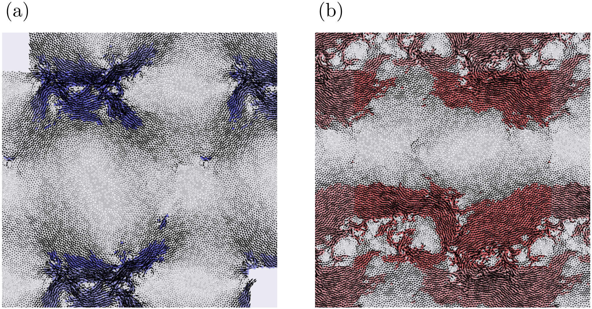
The direct visualization of the displacement field during a precursor and a mainshock provide more insight into the difference between the two event types (see Fig. 6). In particular, the events with the largest avalanche sizes for the same event types are shown. Here, we highlight only mobile particles that are defined according to the participation ratio , where is the magnitude of the displacement vector of particle . The participation ratio provides the fraction of particles that are mobile: if all displacement vectors have the same magnitude, holds, and if only one vector has a nonzero value, holds. We define particles that have the largest magnitudes of displacement vectors as mobile particles. As shown in Fig. 6, even in the largest event, the mobile particles of a precursor exhibit a localized structure, while the mainshock counterpart is system-spanning due to the finite-size effect. Therefore, it is reasonable that precursors are mainly responsible for the intrinsic scale-free power-law regime. We stress that the event in Fig. 6(a) is a chain of multiple STZs.
The qualitative features of mainshocks that have been presented so far are reminiscent of the so-called runaway events observed in the mean-field model of amorphous solids Dahmen et al. 1998; Dahmen et al. 2009. In the mean-field model, such runaway events are expected only when the weakening parameter is positive—in other words, when the system shows brittle responses to an external shear, like metallic glasses. This may seem reasonable, since LJ glasses are sometimes used as a model system of metallic glasses Kob and Andersen 1995. However, our mainshocks exhibit qualitatively different scaling behavior from runaway events. In ref. Carlson et al. 1991, it was reported that runaway events cannot be collapsed by the same scaling exponents as those for the power-law regime. In our case, on the other hand, entire PDFs can be collapsed by a single combination of scaling exponents, as presented in Fig. 3. In this sense, our mainshocks are qualitatively different from runaway events. It is also important to mention that several studies have reported that similar bumps in the PDFs of avalanche sizes can be induced by the inertial effect Salerno et al. 2012; Salerno and Robbins 2013; Karimi et al. 2017. We emphasize that they seem to be different in nature from our mainshocks. This issue is discussed in detail in Appendix B. We would like to note that we are aware of qualitatively similar bumps in PDFs shown in previous works— in both experimental Sun et al. 2010 and numerical works Lin et al. 2014b; Lerner et al. 2014; Zhang et al. 2017. We emphasize that some of them are measured in completely inertialess conditions.
IV Evolution of criticality in the elastic regime
In this chapter, the results in the elastic regime are presented. Specifically, to discuss the issues of criticality and universality independently, we separately present the results of the ensembles of only the initial avalanche events of different samples and of the avalanches collected over the entire elastic regime Shang et al. 2020.
IV.1 Results for unperturbed systems
First, we present the results of the ensembles of only initial avalanche events, which should most strongly reflect the features of unperturbed systems. For each system size, we prepared 4000 independent samples and applied simple shear in an AQS manner until we encountered avalanches. To judge whether the first obtained avalanche event was a precursor or a mainshock, we detected the first two events. The important statistical information is summarized in Fig. 7.
Independent exponents —. The system size dependence of and , which yield the independent exponents and , are shown in Fig. 7(a,b). Although exhibits power-law system size dependence, as in the steady state, (and ) appears rather constant. This result is consistent with the findings reported in ref. Karmakar et al. 2010a and means that criticality is absent in unperturbed systems.
Note that Lin and coworkers have theoretically shown that the pseudogap exponent of an unperturbed system should be universally Lin and Wyart 2016. This means that should be , and our numerical result is reasonably close to this theoretical prediction.
Avalanche size distribution —. Since the statistics are system size-independent, the PDFs of the avalanche sizes of different system sizes are almost identical without any scaling (see Fig. 7(c)). Interestingly, the PDFs still show broad power-law-like shapes. However, because of the absence of criticality, we cannot draw any absolute conclusion as to whether they do indeed follow a power law, although their apparent slopes seem consistent with the value in the steady state, . Nevertheless, we can safely conclude that their apparent slopes are much larger than , which is the prediction of the theory in ref. Franz and Spigler 2017. We also note that the PDFs do not show bumps in the large size regime, unlike the steady state results.
Decomposition of avalanche size distribution —. In Fig. 8, we demonstrate that the PDF of the first event ensemble can also be decomposed into contributions from the precursors and mainshocks. In this case, the mainshocks are not well developed and are completely obscured by the precursors. This is why there is no bump in the PDFs.
Mean square displacements —. The theory in ref. Franz and Spigler 2017 discussed the relation between the energy landscape in the Gardner phase and the statistics of avalanches induced by a very weak perturbation (see Appendix D.2 for a brief summary of the Gardner transition and this theory). Since this theory is based on the replica method, an equilibrium statistical mechanics theory, the first event ensemble that represents the unperturbed system is expected to correspond well to the theoretical situation, although thus far, the avalanches during a small but finite range of strains have been treated as numerical counterparts Franz and Spigler 2017; Shang et al. 2020. Here, we quantify the degree of the similarity to the Gardner phase and show that the presupposition of the full breakage of the replica symmetry in the theory is not satisfied in the case of the first event ensemble in our LJ glass system. This is likely to be one of the reasons why the results are inconsistent with the theoretical predictions Franz and Spigler 2017, such as those for criticality and the value of .
The mean squared displacement (MSD) between different realizations of configurations, , is a quantitative measure of the dissimilarity between two configurations, and its PDF can be used as an order parameter for the Gardner phase33 3 There are several quantitative measures of the similarity or dissimilarity between two configurations. We employed the MSD because it is defined without any parameters. . Here, is the position of particle in the configuration , where states A and B are again used for the states before and after an avalanche event, respectively. According to the mean-field replica theory, in the Gardner phase, the system shows a very wide PDF of the MSD, and importantly, possesses a system-spanning nature reflecting the diverging correlation length Charbonneau et al. 2015; Scalliet et al. 2017. Since the MSD is defined as an intensive variable, the maximum value of the MSD, which corresponds to the system-spanning structure, is expected to be the same across different system sizes if the systems are in the Gardner phase Parisi et al. 2020.
In Fig. 7(d), the PDFs of the MSDs of different system sizes are plotted. Both the maximum and minimum edges of the PDFs shift in accordance with the change in the system size. This behavior is qualitatively different from what we expect for the full PDF of the MSD in the Gardner phase, where the maximum edge should be constant regardless of the system size. Rather, the PDFs are consistent with those of avalanche sizes: they show broad distributions but are not system spanning. The localized (non-system-spanning) tendency can be more explicitly quantified by the total squared displacement (TSD) , which carries information regarding the geometrical size of avalanches. The PDFs of the TSDs of different system sizes nearly overlap each other without any scaling, as is the case for the PDFs of the avalanche sizes (see Appendix E). Therefore, we conclude that the unperturbed systems do not share the same system-spanning vulnerability that is expected for the Gardner phase. Recently, in refs. Scalliet et al. 2017; Hicks et al. 2018; Seoane et al. 2018 the existence of the Gardner phase in physical, finite-dimensional soft-potential systems at rest (unperturbed systems) has been denied. Our results are consistent with these studies.
IV.2 Results of weakly perturbed systems
We conduct the same analysis in the weakly perturbed elastic regime, Shang et al. 2020. We performed simulations of 600, 160, and 50 samples for systems with and , respectively. These sample numbers are chosen to guarantee more than 4000 events for each system size. The important statistical information is summarized in Fig. 9.
Independent exponents —. In this case, all , and show a power-law dependence on the system size (see Figs. 9(a,b)). The value of is larger than that in the steady state because of the well-known non-monotonicity of the pseudogap exponent , which was first predicted theoretically Lin and Wyart 2016 and then numerically confirmed Ozawa et al. 2018; Shang et al. 2020. Nonzero values of and indicate criticality in the elastic regime, in accordance with ref. Shang et al. 2020. However, the estimated values of and do not meet Eq. 20, , since the stationarity condition Eq. 17 is trivially unsatisfied in this regime. We note that the same degree of discrepancy between and in the elastic regime was reported in ref. Shang et al. 2020 44 4 This seems to have nothing to do with the fact that changes abruptly and non-monotonically in the vicinity of because, even if we restrict ourselves to the strain range in which temporarily becomes constant, as in ref. Shang et al. 2020, we observe the same results semi-quantitatively. . We also mention that the fractal dimension in the elastic regime is much less than that in the steady state.
Avalanche size distribution —. The failure of Eq. 17 means that Eq. 18 is not applicable in this regime either55 5 Eq. 18 is expected to be valid even in the elastic regime if we conduct the measurement at a fixed stress level as in ref. Lin et al. 2015. . However, by comparing Eq. 16 and the definition of the exponent , we can derive another form of the scaling relation:
| (21) |
This relation is robustly usable in the elastic regime. The estimation of with this new relation is , and it again describes the small-size regime of the PDFs of the avalanche sizes well (see Fig. 9(c)). Moreover, we stress that this value is very close to the value in the steady state and the mean-field prediction. This result is in agreement with the experimental observations Antonaglia et al. 2014; Denisov et al. 2016.
Decomposition of avalanche size distribution —. The decomposition of the PDF of the avalanche sizes into the contribution from precursors and mainshocks again provide much information (Fig. 10). The PDF of the precursors shows normal power-law behavior with a cutoff, as is the case in the steady state, and moreover, the exponent seems to remain the same. In the elastic regime, unlike the case of the first event ensembles, the mainshocks form a small bump in the large-size regime.
Note that, as presented in Appendix A.2, since mainshocks come into play in this regime, we can fit the data in the crossover regime (which is close to the bump) directly by a power-law curve. The obtained value of the avalanche exponent is quantitatively consistent with that in ref. Shang et al. 2020, , where is the avalanche exponent estimated by potential drops.
Mean square displacements —. The characteristics of the criticality in this regime can be quantified by the PDF of the MSD. As shown in Fig. 9(d), the maximum values of the PDFs of the MSDs of different system sizes still exhibit small discrepancies with each other. Still, reflecting criticality, the PDFs of the TSD are system size-dependent (Appendix E). We stress that if we analyze the displacement field during the avalanche event with the largest avalanche size in the elastic regime, the mobile particles are indeed system spanning. However, the structure of the cluster of mobile particles is less packed than that in the steady state, manifesting its smaller fractal dimension.
IV.3 MSD in the steady state
Finally, we demonstrate that avalanches in the steady state are indeed fully system spanning. We plot the PDFs of the MSD during avalanche events in the steady state in Fig. 11(a). The PDFs of the MSD all have broad distributions, and in particular, the maximum values of different system sizes are the same. This is exactly what we expect for the Gardner phase, as presented above in Sec. IV.1. Therefore, the criticality of the avalanches in binary LJ glass in the steady state is remarkably similar to that in the Gardner phase with respect to the spatial structure, although we are still not sure how tightly we can connect these two concepts because of the lack of a theoretical description. Jin and coworkers Jin et al. 2018 have reported the existence of a shear-induced Gardner transition in a hard sphere system. The extension of their work to softer potentials would be one promising way to test whether our findings have similar characteristics to theirs. Since the MSD is a particle-averaged variable, events with the same TSD result in smaller values of in larger systems. This characteristic leads to a difference in the range of the PDFs depending on the system size: the larger the system becomes, the wider the range becomes (the smaller the smallest MSD becomes). Reflecting this difference in the range, the PDFs of MSDs for different system sizes can be collapsed by scaling as , as shown in Fig. 11(b). In agreement with the PDFs of avalanche sizes, the power-law regime can be seen in a small value regime, and there is a bump in the large value regime. We mention that the precursor/mainshock decomposition is also valid for PDFs of the MSD, and again the bump is composed only of mainshocks (figure not shown).
IV.4 Unified view of avalanche criticality
All the results presented thus far provide a unified understanding of avalanche criticality and universality in the sheared LJ glass system throughout the whole strain regime. While the first event ensemble that represents the unperturbed system is off-critical, criticality emerges in both the elastic regime and the steady state. However, the fractal dimension of the avalanches indicates the quantitative difference between these two strain regimes. In particular, the elastic regime is described by a smaller value of . In this sense, we conclude that criticality gradually grows as shear is applied and becomes fully developed in the steady state, where the fractal dimension is saturated. These observations are all consistent with previous works in the literature Karmakar et al. 2010b; Lin et al. 2015; Seoane et al. 2018; Hicks et al. 2018; Shang et al. 2020.
Once the system becomes critical, the critical exponent remains constant, regardless of the amount of applied strain, and importantly, this value is consistent with the mean-field prediction . The universality of the critical exponent in the elastic regime is then at odds with the theoretical prediction made in ref. Franz and Spigler 2017. This might be partly because the unperturbed system is not in the Gardner phase. Finally, we repeatedly emphasize that the universal values of in each regime in our work are different from those in all previous numerical studiesSalerno et al. 2012; Salerno and Robbins 2013; Zhang et al. 2017; Ozawa et al. 2018; Saitoh et al. 2019; Shang et al. 2020. We consider that non-universal values in previous studies might have been obtained because the crossover regime resulting from the finite-size effects has been analyzed.
V Conclusion and overview
Here, we conducted a thorough investigation of avalanche criticality in a sheared binary LJ glass system by means of atomistic simulations. In particular, by ruling out the ambiguity and arbitrariness that have slipped into measurements in previous studies, we first showed that the critical avalanche exponent in the steady state coincides with the mean-field prediction Dahmen et al. 2009. Our results simultaneously suggest that the scaling function of the avalanche size distribution has a nontrivial bumpy shape. We noticed that there are two qualitatively different avalanche events, and this binariness explains the physical origin of the strange bump in the scaling function. Furthermore, we demonstrated that this bump is likely to be the cause of the nonuniversal results for the critical exponent obtained in previous studies (Appendix A.1).
To investigate the change in criticality and universality due to applied shear, we conducted the same high-precision measurements of avalanche statistics of the first event ensemble, which reflect the properties of the unperturbed system and avalanches in the elastic regime. As a result, we confirmed that the first event ensemble does not exhibit any system-size dependence and thus lacks criticality. This consequence dovetails with the result in ref. Karmakar et al. 2010a. Avalanches in the elastic regime, on the other hand, do display criticality, in accordance with refs. Lin et al. 2015; Shang et al. 2020, and again, the exponent of the power-law part is very close to the mean-field value universally. The value of the critical exponent is in accordance with recent experiments conducted in the elastic regime Antonaglia et al. 2014; Denisov et al. 2016. The criticality in the elastic regime is different from that in the steady state and is characterized by a much smaller value of the fractal dimension . We believe that our results provide a unified picture of avalanche criticality in deformed glasses, for which confusing and seemingly conflicting results have been reported thus far: criticality itself develops along with applied strain, with the exponent of the power-law part remaining constant. In particular, the change in criticality is quantitatively encoded in the fractal dimension , which takes the value of zero in the off-critical unperturbed state and saturates in the steady state.
We employed configurations that are not in the Gardner phase as the initial state in this work, and thus, the starting point itself differs from the theory in ref. Franz and Spigler 2017, where a system in the Gardner phase is considered the initial state. If we find the Gardner phase in physical-dimensional amorphous solid systems with soft potentials, it would be very important and meaningful to conduct the same analyses using the configuration in the Gardner phase as the initial state.
Since we applied shear in an AQS way, the dynamical information could not be accessed. It would also be very important to conduct simulations with a finite-rate shear and investigate the dynamical information, such as the avalanche duration, the avalanche shape and the power spectrum of the stress-drop rate time series.
Acknowledgements.
We thank H. Yoshino, M. Ozawa and H. Ikeda for useful discussions. This work was financially supported by KAKENHI grants (nos. 18H05225, 19H01812, 19K14670, 20H01868, 20H00128, 20K14436 and 20J00802) and partially supported by the Asahi Glass Foundation.Appendix A Comparison with previous works
A.1 Avalanche exponent in the steady state
In this appendix, we discuss the cause of the discrepancies between our result for the avalanche exponent in the steady state and those in previous works with atomistic simulations, Salerno et al. 2012; Salerno and Robbins 2013; Zhang et al. 2017. To this end, we measured by the same method as in the previous works: a direct fitting to the PDFs of avalanche sizes. In particular, we utilized only the data in the large size regime, where the cut-off size resides. As shown in Fig. 12(a), the resulting exponent is located in the middle of the values reported in previous works. Thus, we consider that the cause of the variation in the value of might result from the fact that the non-universal part, which can depend on the details of the systems, has been fitted.
A.2 Avalanche exponent in the elastic regime
Although we used the stress drops for the definition of the avalanche sizes in the main text, the avalanche sizes can also be defined based on the potential energy drops, as follows:
| (22) |
where is the potential energy of state at strain . We use the prime symbol to express the variables of the avalanches defined by Eq. 22.
We also conducted the same direct fitting to the PDF of , avalanche sizes defined based on the potential energy drops, in the elastic regime. The fitting result is and is perfectly consistent with the result in ref. Shang et al. 2020, as shown in Fig. 12(b).
A.3 Scaling collapse
We further demonstrate that the collapse of the data of different sizes by a scaling law is too robust, and thus, unfortunately, it is not reliable enough to guarantee the correctness of the results. In refs. Salerno et al. 2012; Salerno and Robbins 2013; Zhang et al. 2017, the estimated value of is validated by the following scaling law:
| (23) |
where another scaling exponent 66 6 Although we already used the letter to refer to the applied strain, we name this exponent following the definition of the original papers Salerno et al. 2012 to avoid any confusion. is introduced: by scaling by , the power-law parts of the PDFs of different system sizes can be collapsed, as shown in Fig. 12(c). Here, we estimated the value of by using only and , as , as is the case for the other exponents. Note that the authors of refs. Salerno et al. 2012; Salerno and Robbins 2013; Zhang et al. 2017 also confirmed that Eq. 15 holds for the obtained exponents.
What if we try the same scaling collapse with that we obtained by the direct fitting to the data in Fig. 12(a)? The results are shown in Fig. 12(d) (in this case, we use Eq. 23 to obtain the exponent ). As seen here, the power-law parts of different system sizes are collapsed again, even with a different value of . This means that Eq. 23 can be satisfied, unexpectedly, too robustly with multiple values of , and the successful collapse by Eq. 23 alone is not enough evidence for the validity of the obtained value of .
Appendix B Are mainshocks induced by the inertial effect?
Several studies have reported that the introduction of inertia can induce bumps in the PDFs of avalanche sizes Salerno et al. 2012; Salerno and Robbins 2013; Karimi et al. 2017, which are similar to our mainshocks. We discuss the differences among our bumps and those of other studies.
In ref. Karimi et al. 2017, Karimi and coworkers investigated the effect of inertia on the PDFs of avalanche sizes by numerical simulation of a finite-element-based elastoplastic model. They reported that as the effect of inertia becomes stronger, the PDF of the avalanche sizes begins to exhibit a characteristic bump in the large size regime. Since we employed the FIRE algorithm in this work, which can introduce an inertial effect during the energy minimization process, it is possible that our mainshocks share the same origin as the bump reported in ref. Karimi et al. 2017.
According to Karimi et al., in the case of their elastoplastic model, the PDF of the minimum of the local stability shows a bimodal nature when inertia takes effect, and the peak in the large value of is responsible for the bump in the PDF of the avalanche sizes. To check whether our bump has the same physical origin, we also measured the PDF of , which represents the minimum of the local stability in our setup, as discussed in Sec. II.4. As shown in Fig. 13, in our case, the PDF of does not exhibit any salient peaks in the large value regime. This means that the bump observed in our work has a qualitatively different physical origin from that in ref. Karimi et al. 2017. We note that the unimodal shape of is consistent with refs. Karmakar et al. 2010a; Zhang et al. 2017.
Similar inertial effects have also been found in the atomistic simulations in refs. Salerno et al. 2012; Salerno and Robbins 2013. Their results are qualitatively similar to those in our study (the bumps in their PDFs exhibit the same scaling exponents as the ones for the power-law regime). However, the avalanche exponents obtained in the power-law regime are very different ( and in their inertial cases). Therefore, we conclude that the bump in our scaling function is different from those in refs. Salerno et al. 2012; Salerno and Robbins 2013, and thus, our mainshocks are not due to the inertial effect possibly caused by the FIRE algorithm. Indeed, similar bumpy shapes have also been observed in studies where inertialess energy minimization protocols were employed Lin et al. 2014a; Lerner et al. 2014; Zhang et al. 2017.
Appendix C Validation of the strain resolution
In this appendix, we explain how the strain resolution was determined. First, to provide intuition into the importance of the tuning of , we show the results with a fixed crude value of in Fig. 14. Here, the statistical information in the steady state is shown. As shown in Fig. 14(a,b), the dependence of and obviously do not have power-law shapes anymore (the clear deviation of the data of can be recognized). If we turn our attention to the PDF of the avalanche sizes (Fig. 14(c)), the data of the largest system size, , do not reach the peak in the small size regime due to the lack of resolution. If we still attempt to fit the -dependence of and to power-law curves and estimate the exponents , and then from these data, we obtain . Note that, as shown in Fig. 14(d), this exponent does not seem to be inconsistent with the entire curve, and it is very difficult to tell that the result is incorrect if one looks only at the PDF of the avalanche sizes and not at the dependence of . To summarize, the lack of resolution can lead to the deviation of the dependence of and (and presumably as well) from the expected power-law behavior. Moreover, the PDF of the avalanche sizes is truncated from the small size regime where the intrinsic power-law part resides. We carefully tuned the strain resolution so that none of these problems appear.
We further note that to tune the resolution according to the procedure presented above, we need reliable data for small systems as a reference. For this purpose, we conducted simulations for small sizes, , with different resolutions, and confirmed that the PDF converges for (Fig. 15). This is why we employed the value for small systems.
Appendix D Marginal stability
In the last decade, the relation between avalanches in sheared amorphous solids and the marginal stability, which is now expected to be a distinguishing universal feature of amorphous solids, has been discussed Müller and Wyart 2015. In this appendix, we briefly summarize two concepts related to our work.
D.1 Pseudogap exponent
To provide insight into the first concept, the pseudogap exponent, we first introduce a so-called elastoplastic model. In this model, an amorphous solid system is assumed to be an assembly of mesoscale sites. Each site corresponds to a coarse-grained description of a group of particles and has its own local strain , local stress and local yield stress . When the local stress of a site exceeds the corresponding local yield stress, the site will yield locally and give rise to a plastic strain. Such a local yielding is associated with an STZ and thus affects other sites’ local stresses, causing avalanches. The marginal stability can be reflected by, in this context, a pseudogap in the PDF of the local distance to yielding Lin et al. 2014a; the PDF of obeys a power law, , in the limit of . This means that the system is marginally stable against external fields. The existence of the pseudogap in has been confirmed numerically by means of both atomistic simulations and the elastoplastic model, in both two and three dimensions Karmakar et al. 2010a; Lin et al. 2014a. Lin and coworkers derived a scaling relation among the avalanche exponent , the pseudogap exponent and the fractal dimension of the spatial structures of avalanchesLin et al. 2014a, as presented in the main text (see Eq. 18). They validated the scaling relations by numerical calculations with an elastoplastic model.
D.2 Gardner transition
Another distinctive feature of the marginal stability has been predicted by infinite-dimensional mean-field replica theoryCharbonneau et al. 2014. This theory states that when a glassy system crosses a specific border in the parameter space, it experiences full-replica symmetry breakage, and there abruptly emerge infinitesimally different (almost identical) metastable states. This special glassy phase after the transition is distinguished from normal glassy states and is called the Gardner phase. The nature of the Gardner phase is reflected in the infinite hierarchy of metabasins in the energy landscape, and several works have confirmed that the Gardner phase can be observed even in finite physical dimensions in hard sphere systemsBerthier et al. 2016; Jin et al. 2018. However, the parameter space for the Gardner phase is severely limited, and, at least thus far, no work has detected the Gardner phase in a system with softer potentials, such as LJ or the inverse power law, in physical dimensions Scalliet et al. 2017; Hicks et al. 2018; Seoane et al. 2018. Thus, the Gardner aspect of the marginal stability is currently a matter of very active debate Berthier et al. 2019.
Franz and Spigler discussed the relation between avalanche statistics and the Gardner phase in an amorphous solid system with a genuinely short-ranged potential in which the jamming criticality also plays a major role Franz and Spigler 2017. They first formulated, by the replica method, the hierarchical structure of the energy landscape in the Gardner phase. They then treated plastic events under external shear as transitions between metabasins with perturbations induced by shear and showed that, corresponding to the nature of the Gardner phase, such static avalanches are scale-free, and their PDF shows power-law behavior. Note that their theoretical prediction provides the quantitative value of the avalanche exponent and, importantly, argues that the values of are different between systems exactly at the jamming point () and above jamming ().
Appendix E Total squared displacement in the elastic regime
In Secs. IV.1 and IV.2 in the main text, we present the PDFs of the MSDs of the avalanches of the ensembles of the first event and of those in the elastic regime. In this appendix, we present the PDFs of the TSD, , defined as
| (24) |
This gives the geometrical sizes of the events themselves. The results are shown in Fig. 16. In accordance with the avalanche sizes, the TSDs do not show any system size dependence in the case of the first event ensemble (Fig. 16(a)). However, in the case of the elastic regime, we observe a slight system size dependence (Fig. 16(b)).
References
- Sethna et al. (2001) J. P. Sethna, K. A. Dahmen, and C. R. Myers, Nature 410, 242 (2001).
- Faillettaz et al. (2004) J. Faillettaz, F. Louchet, and J.-R. Grasso, Phys. Rev. Lett. 93, 208001 (2004).
- Sethna et al. (1993) J. P. Sethna, K. Dahmen, S. Kartha, J. A. Krumhansl, B. W. Roberts, and J. D. Shore, Phys. Rev. Lett. 70, 3347 (1993), arXiv:9210018 [cond-mat] .
- Dahmen and Sethna (1996) K. Dahmen and J. P. Sethna, Phys. Rev. B 53, 14872 (1996).
- Narayan and Fisher (1993) O. Narayan and D. S. Fisher, Phys. Rev. B 48, 7030 (1993).
- Fisher (1998) D. S. Fisher, Phys. Rep. 301, 113 (1998).
- Palassini and Goethe (2012) M. Palassini and M. Goethe, J. Phys. Conf. Ser. 376, 012009 (2012).
- Dahmen et al. (2009) K. A. Dahmen, Y. Ben-Zion, and J. T. Uhl, Phys. Rev. Lett. 102, 175501 (2009).
- Fisher et al. (1997) D. S. Fisher, K. Dahmen, S. Ramanathan, and Y. Ben-Zion, Phys. Rev. Lett. 78, 4885 (1997), arXiv:9703029 [cond-mat] .
- Dahmen et al. (1998) K. Dahmen, D. ErtaÅ, and Y. Ben-Zion, Phys. Rev. E - Stat. Physics, Plasmas, Fluids, Relat. Interdiscip. Top. 58, 1494 (1998), arXiv:9803057 [cond-mat] .
- Sheikh et al. (2016) M. A. Sheikh, R. L. Weaver, and K. A. Dahmen, Phys. Rev. Lett. 117, 261101 (2016).
- Solé and Manrubia (1996) R. V. Solé and S. C. Manrubia, Phys. Rev. E 54, R42 (1996).
- de Arcangelis et al. (2006) L. de Arcangelis, C. Perrone-Capano, and H. J. Herrmann, Phys. Rev. Lett. 96, 028107 (2006), arXiv:0602014 [q-bio] .
- Friedman et al. (2012) N. Friedman, S. Ito, B. A. W. Brinkman, M. Shimono, R. E. L. DeVille, K. A. Dahmen, J. M. Beggs, and T. C. Butler, Phys. Rev. Lett. 108, 208102 (2012).
- Galam (1997) S. Galam, Phys. A Stat. Mech. its Appl. 238, 66 (1997), arXiv:9702163 [cond-mat] .
- Maloney and Lemaître (2004) C. Maloney and A. Lemaître, Phys. Rev. Lett. 93, 195501 (2004), arXiv:0405096 [cond-mat] .
- Aharonov and Sparks (2004) E. Aharonov and D. Sparks, J. Geophys. Res. Solid Earth 109, n/a (2004).
- Tanguy et al. (2006) A. Tanguy, F. Leonforte, and J. L. Barrat, Eur. Phys. J. E 20, 355 (2006), arXiv:0605397 [cond-mat] .
- Bailey et al. (2007) N. P. Bailey, J. Schiøtz, A. Lemaître, and K. W. Jacobsen, Phys. Rev. Lett. 98, 095501 (2007), arXiv:0702454 [cond-mat] .
- Lerner and Procaccia (2009) E. Lerner and I. Procaccia, Phys. Rev. E 79, 066109 (2009), arXiv:0901.3477 .
- Tsamados (2010) M. Tsamados, Eur. Phys. J. E 32, 165 (2010).
- Heussinger et al. (2010) C. Heussinger, L. Berthier, and J.-L. Barrat, EPL (Europhysics Lett. 90, 20005 (2010), arXiv:1001.0914 .
- Hatano et al. (2015) T. Hatano, C. Narteau, and P. Shebalin, Sci. Rep. 5, 12280 (2015), arXiv:1110.1777 .
- Oyama et al. (2019) N. Oyama, H. Mizuno, and K. Saitoh, Phys. Rev. Lett. 122, 188004 (2019).
- Abed Zadeh et al. (2019) A. Abed Zadeh, J. Barés, and R. P. Behringer, Phys. Rev. E 99, 040901 (2019).
- Manning and Liu (2011) M. L. Manning and A. J. Liu, Phys. Rev. Lett. 107, 108302 (2011).
- Maloney and Lemaître (2006) C. E. Maloney and A. Lemaître, Phys. Rev. E 74, 016118 (2006), arXiv:0510677 [cond-mat] .
- Dahmen et al. (2011) K. A. Dahmen, Y. Ben-Zion, and J. T. Uhl, Nat. Phys. 7, 554 (2011).
- Otsuki and Hayakawa (2014) M. Otsuki and H. Hayakawa, Phys. Rev. E 90, 042202 (2014).
- Sun et al. (2010) B. A. Sun, H. B. Yu, W. Jiao, H. Y. Bai, D. Q. Zhao, and W. H. Wang, Phys. Rev. Lett. 105, 035501 (2010).
- Barés et al. (2017) J. Barés, D. Wang, D. Wang, T. Bertrand, C. S. O’Hern, and R. P. Behringer, Phys. Rev. E 96, 052902 (2017).
- Antonaglia et al. (2014) J. Antonaglia, W. J. Wright, X. Gu, R. R. Byer, T. C. Hufnagel, M. LeBlanc, J. T. Uhl, and K. A. Dahmen, Phys. Rev. Lett. 112, 155501 (2014).
- Denisov et al. (2016) D. V. Denisov, K. A. Lörincz, J. T. Uhl, K. A. Dahmen, and P. Schall, Nat. Commun. 7, 10641 (2016).
- Tong et al. (2016) X. Tong, G. Wang, J. Yi, J. L. Ren, S. Pauly, Y. L. Gao, Q. J. Zhai, N. Mattern, K. A. Dahmen, P. K. Liaw, and J. Eckert, Int. J. Plast. 77, 141 (2016).
- Murphy et al. (2019) K. A. Murphy, K. A. Dahmen, and H. M. Jaeger, Phys. Rev. X 9, 011014 (2019), arXiv:1808.06271 .
- LeBlanc et al. (2016) M. LeBlanc, A. Nawano, W. J. Wright, X. Gu, J. T. Uhl, and K. A. Dahmen, Phys. Rev. E 94, 052135 (2016).
- Maeda and Takeuchi (1978) K. Maeda and S. Takeuchi, Phys. Status Solidi 49, 685 (1978).
- Salerno et al. (2012) K. M. Salerno, C. E. Maloney, and M. O. Robbins, Phys. Rev. Lett. 109, 105703 (2012), arXiv:1204.5965 .
- Salerno and Robbins (2013) K. M. Salerno and M. O. Robbins, Phys. Rev. E 88, 062206 (2013), arXiv:1309.1872 .
- Zhang et al. (2017) D. Zhang, K. A. Dahmen, and M. Ostoja-Starzewski, Phys. Rev. E 95, 032902 (2017).
- Ozawa et al. (2018) M. Ozawa, L. Berthier, G. Biroli, A. Rosso, and G. Tarjus, Proc. Natl. Acad. Sci. 115, 6656 (2018), arXiv:arXiv:1803.11502v1 .
- Saitoh et al. (2019) K. Saitoh, N. Oyama, F. Ogushi, and S. Luding, Soft Matter 15, 3487 (2019).
- Shang et al. (2020) B. Shang, P. Guan, and J. L. Barrat, Proc. Natl. Acad. Sci. U. S. A. 117, 86 (2020), arXiv:1908.08820 .
- Talamali et al. (2011) M. Talamali, V. Petäjä, D. Vandembroucq, and S. Roux, Phys. Rev. E 84, 016115 (2011), arXiv:1103.5017 .
- Budrikis and Zapperi (2013) Z. Budrikis and S. Zapperi, Phys. Rev. E 88, 062403 (2013).
- Lin et al. (2014a) J. Lin, E. Lerner, A. Rosso, and M. Wyart, Proc. Natl. Acad. Sci. U. S. A. 111, 14382 (2014a), arXiv:1403.6735 .
- Budrikis et al. (2017) Z. Budrikis, D. F. Castellanos, S. Sandfeld, M. Zaiser, and S. Zapperi, Nat. Commun. 8, 15928 (2017).
- Ferrero and Jagla (2019a) E. E. Ferrero and E. A. Jagla, Soft Matter 15, 9041 (2019a).
- Ferrero and Jagla (2019b) E. E. Ferrero and E. A. Jagla, Phys. Rev. Lett. 123, 218002 (2019b), arXiv:1905.08771 .
- Liu et al. (2016) C. Liu, E. E. Ferrero, F. Puosi, J.-L. Barrat, and K. Martens, Phys. Rev. Lett. 116, 065501 (2016), arXiv:1506.08161 .
- (51) The maximum value becomes 1.5 if we also include systems under oscillatory shear Otsuki and Hayakawa 2014; Leishangthem et al. 2017.
- (52) Here, only works with finite-size scalings are considered. Before these works, much smaller values were reported, for example in ref. Maloney and Lemaître 2004. Also, refs. Barés et al. 2017 and Saitoh et al. 2019 reported larger values.
- Franz and Spigler (2017) S. Franz and S. Spigler, Phys. Rev. E 95, 022139 (2017), arXiv:1608.01265 .
- Ruscher and Rottler (2019) C. Ruscher and J. Rottler, (2019), arXiv:1908.01081 .
- Karmakar et al. (2010a) S. Karmakar, E. Lerner, and I. Procaccia, Phys. Rev. E 82, 055103 (2010a), arXiv:1008.3967 .
- Lin et al. (2015) J. Lin, T. Gueudré, A. Rosso, and M. Wyart, Phys. Rev. Lett. 115, 168001 (2015), arXiv:1505.02571 .
- Berthier et al. (2019) L. Berthier, G. Biroli, P. Charbonneau, E. I. Corwin, S. Franz, and F. Zamponi, J. Chem. Phys. 151, 010901 (2019).
- Allen and Tildesley (1987) M. P. Allen and D. J. Tildesley, Computer simulation of liquids (Oxford University Press, 1987).
- Bitzek et al. (2006) E. Bitzek, P. Koskinen, F. Gähler, M. Moseler, and P. Gumbsch, Phys. Rev. Lett. 97, 170201 (2006).
- Karmakar et al. (2010b) S. Karmakar, E. Lerner, I. Procaccia, and J. Zylberg, Phys. Rev. E 82, 031301 (2010b).
- Kob and Andersen (1995) W. Kob and H. C. Andersen, Phys. Rev. E 52, 4134 (1995), arXiv:9505118 [cond-mat] .
- Carlson et al. (1991) J. M. Carlson, J. S. Langer, B. E. Shaw, and C. Tang, Phys. Rev. A 44, 884 (1991).
- Karimi et al. (2017) K. Karimi, E. E. Ferrero, and J.-L. Barrat, Phys. Rev. E 95, 013003 (2017), arXiv:1610.00533 .
- Lin et al. (2014b) J. Lin, A. Saade, E. Lerner, A. Rosso, and M. Wyart, EPL (Europhysics Lett. 105, 26003 (2014b), arXiv:1307.1646 .
- Lerner et al. (2014) E. Lerner, N. P. Bailey, and J. C. Dyre, Phys. Rev. E 90, 052304 (2014), arXiv:1405.0156 .
- Lin and Wyart (2016) J. Lin and M. Wyart, Phys. Rev. X 6, 011005 (2016), arXiv:1506.03639 .
- (67) There are several quantitative measures of the similarity or dissimilarity between two configurations. We employed the MSD because it is defined without any parameters.
- Charbonneau et al. (2015) P. Charbonneau, Y. Jin, G. Parisi, C. Rainone, B. Seoane, and F. Zamponi, Phys. Rev. E 92, 012316 (2015), arXiv:1501.07244 .
- Scalliet et al. (2017) C. Scalliet, L. Berthier, and F. Zamponi, Phys. Rev. Lett. 119, 205501 (2017).
- Parisi et al. (2020) G. Parisi, P. Urbani, and F. Zamponi, Theory of Simple Glasses (Cambridge University Press, 2020).
- Hicks et al. (2018) C. L. Hicks, M. J. Wheatley, M. J. Godfrey, and M. A. Moore, Phys. Rev. Lett. 120, 225501 (2018).
- Seoane et al. (2018) B. Seoane, D. R. Reid, J. J. de Pablo, and F. Zamponi, Phys. Rev. Mater. 2, 015602 (2018).
- (73) This seems to have nothing to do with the fact that changes abruptly and non-monotonically in the vicinity of , since even if we restrict ourselves to the strain range at which becomes constant temporarily, as in ref. Shang et al. 2020, we observe the same results semi-quantitatively.
- (74) Eq. 18 is expected to be valid even in the elastic regime if we conduct the measurement at a fixed stress as in ref. Lin et al. 2015.
- Jin et al. (2018) Y. Jin, P. Urbani, F. Zamponi, and H. Yoshino, Sci. Adv. 4, eaat6387 (2018).
- (76) Although we already used the letter to refer to the applied strain, we also name this exponent following the definition of the original paper Salerno et al. 2012 to avoid confusion.
- Müller and Wyart (2015) M. Müller and M. Wyart, Annu. Rev. Condens. Matter Phys. 6, 177 (2015), arXiv:1406.7669 .
- Charbonneau et al. (2014) P. Charbonneau, J. Kurchan, G. Parisi, P. Urbani, and F. Zamponi, Nat. Commun. 5, 3725 (2014), arXiv:1404.6809 .
- Berthier et al. (2016) L. Berthier, P. Charbonneau, Y. Jin, G. Parisi, B. Seoane, and F. Zamponi, Proc. Natl. Acad. Sci. U. S. A. 113, 8397 (2016), arXiv:1511.04201 .
- Leishangthem et al. (2017) P. Leishangthem, A. D. S. Parmar, and S. Sastry, Nat. Commun. 8, 14653 (2017), arXiv:1612.02629 .