XL-MIMO Energy-Efficient Antenna Selection under Non-Stationary Channels

In XL-MIMO systems, spatial non-stationarities occur frequently since typically $d_{\max}<L$, what means that a given user probably sees only a small part of the antenna array. The propagation environment contains numerous objects reflecting the signal, which are called scattering points. Each scattering point has an associated VR. Herein, we assume that each user can see the antenna array through $N_{\text{c}}$ different VRs. The $i$-th VR that is visible to the $k$-th user extends from the $c_{ik}$-th to the $(c_{ik}+N_{ik})$-th antenna and is denoted by $\mathcal{C}_{ik}=\{c_{ik}\ ,\ c_{ik}+1\ ,\ \dots\ ,\ c_{ik}+N_{ik}\}$. These VRs may overlap, and the set $\mathcal{C}_{k}=\mathcal{C}_{1,k}\ \cup\ \dots\ \cup\ \mathcal{C}_{N_{\text{C}},k}$ contains the indices of the antennas that are visible to the $k$-th user. Considering that each user sees the antenna array through more than one VR, it is a way of taking into account that not only one subset of the array containing contiguous antenna elements may be visible. Indeed, the mobile user may see more than one portion of the array. For instance, if $M=100$ in Figure 2, it may see antennas 10 to 20 and 25 to 40, which means there is something in the propagation environment preventing the signal from reaching antennas 21 to 24.

In general, the distances between a given user and all the BS antennas are considered to be the same. However, in the XL-MIMO scenario, as the length of the antenna array is not negligible, the pathloss varies throughout the array, mainly when $d_{\max}\ll L$. The pathloss coefficient between the $m$-th antenna and the $k$-th user is given by:

where $\gamma\geq 2$ is the pathloss exponent and $b_{0}$ determines the median channel gain at a reference distance of 1 m[6]. The parameters $b_{0}$ and $\gamma$ are functions of the carrier frequency, antenna gains, and vertical heights of the antennas, which are derived from fitting (1) to measurements [6]. Finally, the channel vector $\textbf{h}_{k}=[h_{1k}\penalty\ \dots\penalty\ h_{Mk}]^{\text{T}}$ between the BS and the $k$-th user is given by:

where $\textbf{b}_{k}$ is a vector whose $m$-th element is $b_{mk}$, and $\overline{\textbf{h}}_{k}$ is the independent Rayleigh fading component, which accounts for the short-scale fading and follows a complex-Gaussian distribution $\overline{\textbf{h}}_{k}\sim\mathcal{CN}(\textbf{0}_{M},\textbf{I}_{M})$. The coefficient $a_{mk}=[\textbf{a}_{k}]_{m}$ indicates whether the $m$-th antenna is visible to the $k$-th user ($a_{mk}$ = 1) or not ($a_{mk}$ = 0), and is given by:

We assume the channel is estimated via UL synchronous pilot transmission, which means that all users simultaneously send pilot sequences from the same pilot codebook. They have length $\tau_{\text{p}}$ and form an orthogonal set. Herein, it is assumed that each user is assigned a different pilot sequence. Then, the pilot sequences’ set is $\bm{\Psi}=[\bm{\psi}_{1}\ldots\bm{\psi}_{K}]\in\mathbb{C}^{\tau_{\text{p}}\times K}$ and the orthogonality condition states that $\bm{\Psi}^{\text{H}}\bm{\Psi}=\tau_{\text{p}}\textbf{I}_{\tau_{\text{p}}}$, i.e.:

During the UL pilot transmission, the $k$-th user transmits the pilot sequence $\bm{\psi}_{k}\in\mathbb{C}^{\tau_{\text{p}}}$, with transmit power $p_{\text{p}}$. The elements of $\bm{\psi}_{k}$ are scaled by $\sqrt{p_{\text{p}}}$, forming the signal $\textbf{s}_{k}=\sqrt{p_{\text{p}}}\bm{\psi}_{k}^{\text{H}}$, to be transmitted over $\tau_{\text{p}}$ UL samples. As a result, the BS receives the signal $\textbf{Y}^{\text{p}}\in\mathbb{C}^{M\times\tau_{\text{p}}}$:

where $\textbf{N}^{\text{p}}\in\mathbb{C}^{M\times\tau_{\text{p}}}$ is the noise matrix at the receiver of the BS with i.i.d. entries following a complex normal distribution with zero mean and variance $\sigma_{\text{UL}}^{2}$.

The received signal $\textbf{r}\in\mathbb{C}^{M}$ at the BS during the UL data transmission is:

where $x_{k}$ is the signal sent by the $k$-th user and $\textbf{n}\sim\mathcal{CN}(\mathbf{0}_{M},\sigma_{\text{UL}}^{2}\textbf{I}_{M})$ contains the noise received at the BS antennas. By utilizing a suitable combining vector, $\textbf{v}_{k}\in\mathbb{C}^{M}$, the BS detects the $k$-th user’s signal as follows:

Herein we consider the two simplest types of linear processing for receive combining: zero-forcing (ZF) and maximum-ratio (MR), which are respectively defined by:

and

where the matrix $\textbf{V}=[\textbf{v}_{1}\dots\textbf{v}_{K}]$ is the collection of the combining vectors. ZF induces considerably smaller intra-cell interference than MR, yielding significantly better performance under interference-limited conditions, which is normally the case. On the other hand, it increases computational complexity significantly when employing large antenna arrays, due to multiplications of complex numbers, and when serving a great number of users, due to the size of the $K\times K$ matrix that is inverted[3, 6]. Due to these particularities, it is interesting to compare the system performance in terms of SE and EE considering such linear processing techniques.

The channels are practically constant within a coherence block, while the signals and noise take new realization at every sample. Then, the instantaneous SINR is actually an expectation over one coherence block, what means that $p_{k}^{\text{UL}}=\mathbb{E}\{|x_{k}|^{2}\}$ - which is the UL transmit power of the $k$th user - and $\sigma_{\text{UL}}^{2}$ will be taken instead of the instantaneous values of $|x_{k}|^{2}$ and $|n_{k}|^{2}$, respectively. Thus, one can define the SINR of the $k$th user during the UL data transmission as

As a result, the UL ergodic spectral efficiency is defined by[6]:

In the DL, the information to be transmitted by the BS to the $k$-th user, $x_{k}$, needs to be precoded, by using the precoding vector $\textbf{w}_{k}$. The signal to be transmitted, denoted by $\textbf{s}\in\mathbb{C}^{M}$, is generated as:

We denote the matrix containing the collection of the precoding vectors by $\textbf{W}=[\textbf{w}_{1}\penalty\ \cdots\penalty\ \textbf{w}_{K}]\in\mathbb{C}^{M\times K}$. The UL-DL duality motivates a simple precoding design principle: selecting the DL precoding vectors as the normalized version of their respective combining vectors[6]:

Assuming no receive combining, user $k$ receives the signal:

where the received noise follows the distribution $n_{k}\sim\mathcal{CN}(0,\sigma_{\text{DL}}^{2})$. Analogously to (12) for the UL, the SINR of the $k$th user in the DL data transmission is defined as:

where $p_{k}^{\text{DL}}$ is the downlink transmit power assigned for user $k$, i.e., $\sqrt{p_{k}^{\text{DL}}}$ scales the vector $\textbf{w}_{k}$, which has unit norm. Finally, the DL ergodic spectral efficiency is given by[6]:

First, Algorithm 1 computes the vector $\bm{\theta}_{k}\in\mathbb{C}^{M}$, which is a quantitative indicator of the quality of the channel between the $k$-th user and each of the $M$ antennas as:

where $\hat{h}_{mk}=[\hat{\textbf{h}}_{k}]_{m}$ and $\theta_{mk}=[\bm{\theta}_{k}]_{m}$. A high signal intensity may be obtained when $|\hat{h}_{mk}|^{2}$ is strong. Selecting the $N$ strongest $\theta_{mk}$ values among $m=1,\ldots,M$ in (19) for each user, provides the highest received normalized power (HRNP) antenna selection criterion. On the other hand, the terms $|\hat{h}_{mi}|^{2}$, $i\neq k$, are related to the interference intensity. Higher $\theta_{mk}$ values are therefore associated to higher SINRs on the signal detection, as defined by the equations (12) and (17), and consequently higher SE and EE.

As the set $\mathcal{D}_{k}$ contains the indices of the antennas that are active for the $k$th user, the superset $\mathcal{D}=\mathcal{D}_{1}\cup\dots\cup\mathcal{D}_{K}$ contains all the indices of the antennas that are active for any user. The number of elements in $\mathcal{D}$, denoted by $N_{\text{act}}$, corresponds to the total number of active elements of antenna. Notice that the rows of the combining and the precoding matrices corresponding to the antennas whose indices are not in the set $\mathcal{D}_{k}$ are set equal zero.

We first address the complexity of computing the ZF combining vectors (line 13, Algorithm 1). Recalling that $\hat{\textbf{H}}_{k}\in\mathbb{C}^{N\times K}$, the multiplication of $\hat{\textbf{H}}_{k}^{\text{H}}$ by $\hat{\textbf{H}}_{k}$ requires $\frac{K^{2}+K}{2}N$ complex multiplications²² 2 Being $\textbf{A}\in\mathbb{C}^{a\times b}$ and $\textbf{B}\in\mathbb{C}^{b\times c}$, the multiplication AB requires $ac$ inner products between $b$-length vector, what corresponds to $abc$ complex multiplications. However, if $\textbf{B}=\textbf{A}^{\text{H}}$, the Hermitian symmetry is utilized. Thus, only the $a$ diagonal elements of $\textbf{A}\cdot\textbf{B}$ and half of the $a^{2}-a$ off-diagonal elements need to be computed, what gives $\frac{a^{2}+a}{2}b$ complex multiplications[6]., using the Hermitian symmetry. When the inverse of a matrix is multiplied by another matrix, the $\textbf{LDL}^{\text{H}}$ decomposition can be used to achieve an efficient hardware implementation [6]. The decomposition of $\hat{\textbf{H}}_{k}^{\text{H}}\hat{\textbf{H}}_{k}$ requires $\frac{K^{3}-K}{3}$ complex multiplications[6]. Finally, we need to multiply the matrix $\hat{\textbf{H}}_{k}$ by the $k$-th column of the matrix $(\hat{\textbf{H}}_{k}^{\text{H}}\hat{\textbf{H}}_{k})^{-1}$, which requires $KN$ complex multiplications plus $K$ complex divisions to compute $\textbf{D}^{-1}$[6, 18]. Considering complex multiplications and complex divisions to correspond to 3 and 7 flops³³ 3 Considering $x=a+jb$ and $y=c+jd$, then $\frac{x}{y}=\frac{xy^{*}}{yy^{*}}=\frac{xy^{*}}{|y|^{2}}$, while the computation of $xy^{*}$ requires 3 real multiplications. The computation of $|y|^{2}=c^{2}+d^{2}$ requires 2 real multiplications. Finally, the complex division $\frac{xy^{*}}{|y|^{2}}$ corresponds to 2 real divisions, making a total of 7 real operations., respectively, the computation of the combining vector $\textbf{v}_{k}$ has a complexity of $3\left(\frac{K^{2}+K}{2}N+\frac{K^{3}-K}{3}+KN\right)+7K$ flops per coherence block. Thus, the computational complexity to obtain the whole combining matrix V is given by:

As defined in (11), MR combining does not require multiplications or divisions, because it is given directly from the channel estimates (from Algorithm 1, one can see that the $k$-th column of the MR combining matrix is simply a copy of the $k$-th column of $\hat{\textbf{H}}_{k}$). However, in practical implementations, we typically normalize the combining vector such that $\textbf{v}_{k}^{\text{H}}\textbf{h}_{k}$ in front of the desired signal $x_{k}$ is close to one. Thus, this normalization requires 1 complex division per user[6], resulting in a total of $7K$ flops per coherence block. Finally, the complexity of computing the MR combining matrix is given by:

The precoding vectors ($\textbf{w}_{k}$) are chosen as the normalized versions of the combining vectors ($\textbf{v}_{k}$), as described in equation (15). The computation of $||\textbf{v}_{k}||$ requires $2N$ real multiplications⁴⁴ 4 Consider the complex vector $\textbf{x}=[x_{1},\dots,x_{N}]$. The computation of $||\textbf{x}||=\sqrt{\sum\limits_{\begin{subarray}{c}n=1\end{subarray}}^{N}|x_{n}|^{2}}$ depends on previously obtaining $|x_{m}|^{2}$. Being $x_{n}=a_{n}+jb_{n}$ a complex scalar, $|x_{n}|^{2}=a_{n}^{2}+b_{n}^{2}$ requires 2 real multiplications and 1 real sum. Therefore, the computation of $||\textbf{x}_{k}||$ requires $2N$ real multiplications. and the division of $\textbf{v}_{k}$ by $||\textbf{v}_{k}||$ also requires $2N$ real divisions⁵⁵ 5 The division of a complex scalar $x=a+jb$ by a real scalar $c$ requires 2 real divisions. Therefore, the division of x by $||\textbf{x}||$ requires $2N$ real divisions., resulting in a total of $4N$ flops. Thus, the computation of the precoding matrix has a complexity of:

Notice that the rows of the combining and the precoding vectors of the user $k$ that correspond to the antennas whose indices are not in the set $\mathcal{D}_{k}$ are set equal zero. It reduces the complexity to obtain $y_{k}$, as in (9), because the BS will use $N$ elements of the vectors $\textbf{v}_{k}$ and r, instead of $M$ elements, resulting in $3N$ flops. This procedure is repeated $\tau_{\text{u}}$ times per coherence block. Similarly, the complexity to precode the information during DL, $\textbf{w}_{k}x_{k}$, following (14), is reduced since the BS only uses $N$ elements of the vector $\textbf{w}_{k}$, also resulting in $3N$ flops. This task is performed $\tau_{\text{d}}$ times per coherence block. Finally, the computational complexity associated to the reception and transmission of the information, in number of flops per coherence block, is:

To obtain $\theta_{mk}$ in (19), the BS computes $2K$ real multiplications and 1 real division. As there are $M$ antennas and $K$ users, the associated complexity is:

Finally, the total signal processing computational complexity, in flops per coherence block, when employing MR and ZF processing in the context of XL-MIMO antenna selection is given respectively by:

and

Hence, if antenna selection (AS) procedure is not applied, the complexities given in (20), (22) and (23) will be higher, since all the $M$ antennas always will be active for all the $K$ users, i.e., $N=M$.

The other terms of the model represented in (32) account for the power consumption of the transceiver chains ($P_{\text{TC}}$), the channel estimation process ($P_{\text{CE}}$), the channel coding and decoding units ($P_{\text{C/D}}$), the load-dependent backhaul ($P_{\text{BH}}$) and the linear processing at the BS ($P_{\text{LP}}$). Each of these terms depends on at least one of the main system parameters: $M$, $K$ and the ergodic spectral efficiency (SE).

The power consumption of the transceiver chains ($P_{\text{TC}}$) involves the power consumed by the BS local oscillator ($P_{\text{LO}}$), the power required by the circuit components (converters, mixers and filters) of each BS antenna ($P_{\text{BS}}$) and the power necessary to run the circuit components (mixers, filters, amplifiers and oscillator) of each single-antenna user ($P_{\text{UE}}$), as described by the equation

The computational complexity associated to the channel estimation process is given by the equation (7). Hence, the resulting power consumption is given by⁶⁶ 6 As each coherence block contains $\tau_{\text{c}}$ symbols per second, $B/\tau_{\text{c}}$ is the number of coherence blocks per second. If a given signal processing has a computational complexity denoted by $C$, representing the number of flops per coherence block, and $L$ is the computational efficiency, representing the number of flops per Joule of energy, then $\frac{C}{L}$ represents the energy consumption per coherence block. Therefore, the associated power consumption is $\frac{BC}{\tau_{\text{c}}L}$.:

where $L_{\text{BS}}$ is the computational efficiency at the BS, in [flop/s W]. Similarly, the total signal power consumption is given by:

The power consumed by the channel coding and decoding units is defined as

which increases linearly with the actual rates. $\mathcal{P}_{\text{COD}}$ and $\mathcal{P}_{\text{DEC}}$ are the coding and decoding power densities, respectively, in $\left[\frac{\text{watt}}{\text{bit/s}}\right]$. For simplicity, $\mathcal{P}_{\text{COD}}$ and $\mathcal{P}_{\text{DEC}}$ are assumed to be the same in both UL and DL.

The load-dependent backhaul power consumption, necessary for the UL and DL data transmission between the BS and the core network, is modeled as

where $\cal{P}_{\text{BT}}$ is the backhaul traffic power density, in $\left[\frac{\text{watt}}{\text{bit/s}}\right]$. There is also a load-independent backhaul power consumption, which can be included in $P_{\text{FIX}}$.

In our simulations, the antenna array contains $M$ = 100 antenna elements and each user sees the array through 3 different VRs, i.e., $N_{\text{c}}=3$. Furthermore, $N_{ik}$ is taken as a uniform random variable distribution over the interval $[0.1M,0.3M]$, while the index of the first antenna that is inside this VR, denoted by $c_{ik}$, follows a uniform distribution in the interval $[1,M-N_{ik}]$.

The set $\mathcal{C}_{k}=\mathcal{C}_{1,k}\ \cup\ \dots\ \cup\ \mathcal{C}_{N_{\text{C}},k}$ contains the indices of the antennas that sees the $k$-th user. Thus, the number of elements in $\mathcal{C}_{k}$ corresponds to the total number of antennas seen by user $k$. We obtained this value numerically from our simulations. As well as the other numerical results presented in the paper, this value was averaged out of 1,000 random realizations, obtaining the average number of active antennas for the $k$-user as $|\mathcal{C}|=55.8$. It means that approximately 56 antennas are seen by each user, on average. Also from our simulations, we found that, when $K$ = 4, each antenna sees an average of 2.23 users, while for $K$ = 40 this number goes to 22.3, resulting in higher interference levels.

Moreover, we assume equal power allocation (EPA), what means the transmit power is the same for all users. Hence, during the UL data transmission, $p_{k}^{\text{UL}}=p_{\text{UL}}$, while during the DL data transmission, the total available transmit power at the BS, $P_{\text{DL}}$, is equally divided among the $K$ users, so that the power allocated to the $k$-th user is $p_{k}^{\text{DL}}=P_{\text{DL}}/K$. We have adopted $p_{\text{P}}=p_{\text{UL}}$ = 0.1 W and $P_{\text{DL}}$ = 1 W. Although the position of the users (and consequently the pathloss), the short-scale fading and the VRs are random variables, the numerical results are statically relevant because they represent an average over 1,000 realizations.

Figure 3 shows an example of the XL-MIMO system user spatial distribution, where $K=4$ and $M=16$, for simplicity. Each triangle represents one of the 16 BS antennas, while each colored circle represents one of the 4 mobile users, which are randomly distributed over a rectangular area. Taking a random channel realization, the portion of the array that each user sees is indicated by the horizontal line with its correspondent color. User 1, for example, sees the antennas 1 to 10, while user 2 sees the antennas 9 to 15, excepting the antenna 13. This fragmentation of the VR into two parts may occur if any object is blocking the signal in that region.

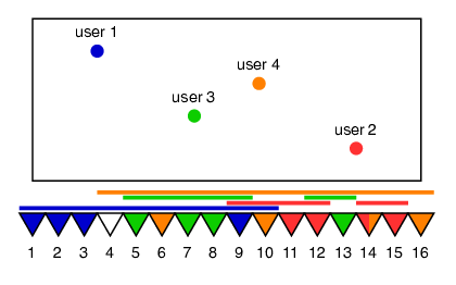
In this example, the algorithm was set up to define $N=4$ antennas to communicate with each user. In the figure, the triangle that represents a given antenna $m$ is painted with the user $k$ color if user $k$ sees antenna $m$. For example, antennas 1, 2, 3 and 9, which are in blue, were designated to communicate with user 1. Notice that all these 4 antennas are part of the VR of user 1. Although the signal from user 1 probably achieves the antennas 4 to 8 with higher intensity than antenna 9, choosing one of these antennas would increase the received interference power, mainly due to user 3. Observe that antenna 4 is not active, while antenna 14 serves users 2 and 4, simultaneously. Therefore, considering that only one antenna was designated to communicate with 2 users at the same time, we can say that the algorithm succeeded in avoiding the interference from other users to affect the SINR while reducing the computational complexity.

In the following, we present numerical results demonstrating how the number of active antennas per user ($N$) influences the system performance, in terms of throughput and EE, and the resource consumption, in terms of computational complexity and power consumption. From these results, we can see the advantages of appropriately selecting the antennas subset (AS strategy) against utilizing the whole antenna array strategy to serve all users at the same time (no-AS strategy). To refine the comprehension upon these results, which depend on the processing scheme (MR or ZF), Fig. 4 provides, for two different scenarios ($K$ = 4 and $K$ = 40), valuable insights on how $N$ influences the received signal, interference and noise power, during the UL and during the DL, which are given by the definitions in Table II.

Figures 4(a) and 4(b) compare the UL signal, interference and noise power, as given by the definitions Def. 1 to 3, when the number of users is 4 and 40, respectively. When $N<K$, it is not possible to execute ZF, due to singularity problems with the matrix $\hat{\textbf{H}}^{\text{H}}\hat{\textbf{H}}$. First, one can see that the received power levels of ZF are higher than of MR. The reason is that ZF receive combining is the pseudoinverse of $\hat{\textbf{H}}$ (recall that the elements of the channel matrix include the pathloss effect), while MR combining is simply a copy of $\hat{\textbf{H}}$. Second, by comparing Figures 4(a) and 4(b), one can observe that,as expected, when $K$ = 40, the received interference power ($\mathcal{I}_{\text{UL}}$) is higher than when $K$ = 4, because the selectivity of the receive combining deteriorates. Third, looking at the MR curves, one can verify that, by selecting more antennas to be active for each user, the received signal power increases, but so does the interference and noise power. It does not occur when employing ZF combining. By increasing $N$, ZF performs better at reducing the interference and noise power, because the receive combining becomes more selective. Fourth, if the channel estimates are reliable, ZF combining will force the average received signal power ($\mathcal{S}_{\text{UL}}$) to $p_{\text{UL}}$, as $|\textbf{v}_{k}^{\text{H}}\textbf{h}_{k}|^{2}=1$, from the definition of ZF combining. It can be observed in the figure, what attests that the channel estimation predicted by eq. (6a) provides good estimates.

Unlike the UL case, during the DL (see Fig. 4(c) and 4(d)), the average received noise, $\mathcal{N}_{\text{DL}}$, does not depend on the precoding scheme (compare Def. 3 and 6). Another important point is that the desired signal power ($\mathcal{S}_{\text{DL}}$) is the same magnitude order for both MR and ZF, because the precoding vectors are normalized, unlike the combining vectors. Finally, as the total available DL transmit power ($P_{\text{DL}}$) is distributed among the $K$ users, the individual DL transmit power ($p_{k}^{\text{DL}}$) is inversely proportional to $K$. That is why the average signal and interference power are smaller in Fig. 4(d) than in Fig. 4(c). The exception is $\mathcal{I}_{\text{DL}}$ when employing MR precoding, which is less efficient than ZF at eliminating the interference.

Fig. 4(e) and 4(f) depict the UL, DL and UL+DL throughput, given by $B\cdot\text{SE}_{\text{UL}}$, $B\cdot\text{SE}_{\text{DL}}$ and $B\cdot\text{SE}$, respectively. The throughput resulting from the no-AS strategy can be obtained in the point $N$ = 100. Thus, we can see that in a scenario with few active users, the AS strategy improves considerably the system throughput when using MR. On the other side, considering the $K$ = 40 scenario, the high interference levels deteriorate the selectivity of MR combining and precoding, and the AS strategy cannot improve the throughput. The same behavior is observed with ZF processing, independently of the number of users. However, as the array is physically large and the users have a VR corresponding to around 50% of the array, on average (as discussed in the beginning of Section V-A), increasing $N$ beyond $M/2$ can barely improves the throughput. Thus, by taking $N$ close to $M/2$, we can obtain almost the same throughput achieved with the no-AS strategy, as shown in Figures 4(e) and 4(f), while benefiting from lower computational complexity and consequently lower power consumption.

While $\mathcal{D}_{k}$ contains the indices of the $N$ antennas that are active for user $k$, the set $\mathcal{D}$ contains the indices of antennas $N_{\text{act}}$ that are active for any of the $K$ users. Fig. 5 addresses the dependency of $N_{\text{act}}$ on $N$. In the scenario with 4 users, the whole antenna array is expected to be active when $N\geq 34$, approximately. When $K$ = 40, $N_{\text{act}}$ scales faster than when $K$ = 4, and reaches the limit of 100 when $N\approx 8$. If a small $N$ is sufficient to substantially increase the EE or throughput, one will benefit from the reduced circuit power consumption, as $P_{\text{TC}}$ is proportional to $N_{\text{act}}$, according to (33). It can be evidenced by Fig. 6(c) and 6(d) that with small values of $N$, the AS strategy provides considerable reduction on the power consumption comparing to the entire antenna array activation (no-AS strategy).

Table III provides a quantitative analysis of the impact of the proposed HRNP-based AS scheme on the overall XL-MIMO computational complexity, given by $C=C_{\text{CE}}+C_{\text{TSP}}$. The complexity associated to the no-AS strategy can be obtained from (20), (21), (22) and (23) by simply replacing $N$ with $M$ in these equations, and cancelling $C_{\text{SP},\theta}$ out in (25) and (26). The complexities are in the unit of [flop/s], which is given by $BC/\tau_{\text{c}}$, recalling that $C$ is measured in flop per coherence block [fpcb]. The first three columns of the table define four scenarios, with different values of $M$, $N$ and $K$. The other columns contain the complexity associated to each processing scheme (MR and ZF), when using or not the AS algorithm. Notice that the algorithm yields very lower complexities, which is particularly advantageous in high system dimensions (many BS antennas and many users). Also, although providing lower throughput than ZF, one can benefit from using MR due to its much smaller complexity. However, in the fourth scenario, the AS’s complexity surpasses the no-AS’s when employing MR, because $C_{\text{SP},\theta}$ is the only term of $C_{\text{TSP}}$ that is proportional to $K^{2}$. It does not occur with ZF, as the term $C_{\text{SP-C}}^{\text{UL-ZF}}$ is much more significative than $C_{\text{SP},\theta}$.

Fig. 6(a) shows the linear dependency of the computational complexity on $N$ and the remarkable computational complexity reduction provided by the adopted AS strategy. As a consequence, there is also a reduction in the total power consumption, defined as $P_{\text{tot}}=P_{\text{TX}}^{\text{UL}}+P_{\text{TX}}^{\text{DL}}+P_{\text{TX}}^{\text{tr}}+P_{\text{CP}}$, as depicted in Fig. 6(c). Moreover, Fig. 6(b) reveals a significant complexity increase when the number of active users grows from 4 to 40. Furthermore, by avoiding all antennas to be simultaneously active, the adopted HRNP-AS strategy in eq. (19) reduces the transceiver chains power consumption⁷⁷ 7 Notice that from (33), power consumption is linearly dependent on $N_{\text{act}}$., and consequently the total power consumption, as indicated in Fig. 6(c) and 6(d). As a final remark on the advantage in adopting the HRNP-AS strategy is the operation point where the AS power consumption curves meet the no-AS curves is very close to the point where the average number of active antennas meet $M$ in Fig. 5.

Fig. 7 confirms the EE improvement when AS strategy based on highest received power is adopted. Under reduced loading scenario ($K=4$), the EE is maximized when $N=6$ and $N=1$ for ZF and MR, respectively. It demonstrates that the HRNP-AS strategy can guarantee huge EE improvements in a scenario with few users, while reducing considerably the power consumption and the computational burden, as discussed above. On the other hand, results in Fig. 7(b) demonstrate that, the AS strategy cannot improve the EE considerably when XL-MIMO operates under high loading scenarios ($K=40$). However, the HRNP-based AS strategy is still advantageous over the no-AS strategy, as it still provides a considerable complexity reduction. Thus, regardless of the number of users, it is not reasonable to use the whole antenna array to serve all users if about half of the antennas is sufficient to achieve a remarkable EE increasing with a lower computational complexity.

Table IV shows the optimal number of selected antennas ($N^{*}$) that maximizes the EE, when employing both linear MR or ZF filtering. According to the data, $N^{*}$ is strongly influenced by the number of active users $K$. As a rule of thumb, when the number of active users is up to a limit, namely $K_{\text{max}}$, the EE is maximized when the AS algorithm selects less than $10\%$ of the antenna array to communicate with each user, i.e., $N^{*}\leq M/10$. From the data in Table IV, we see that $K_{\text{max}}=20$ for MR and $K_{\text{max}}=6$ for ZF.

Figs. 8(a), 8(b), 8(c) and 8(d) depict the EE, throughput, power consumption and computational complexity, respectively, for the proposed HRNP-AS and no-AS strategy assuming $N=N^{*}$. If the system operates under the bound $K\leq K_{\text{max}}$, the HRNP-AS strategy provides an increasing in the EE and simultaneously reduces the power consumption and the computational burden, while the throughput is very close to the obtained with the no-AS strategy.

Besides, when increasing $K$ until it is close to $K_{\text{max}}$, the EE gradually decreases until it meets the no-AS strategy EE curve. It occurs because taking $N\leq M/10$ is no longer enough to mitigate the interference. Besides, from the point $K=K_{\text{max}}$, $N^{*}$ suddenly jumps to about 50 or 60% of the ULA array size, $M=100$. Finally, when the XL-MIMO system operates over the maximum number of user bound, $K>K_{\text{max}}$, the AS-strategy is no longer able to improve the EE and simultaneously reduce the power consumption considerably. However, it is still advantageous when compared to the all-antennas activation strategy, as it is still able to reduce the computational burden.

References

- [1] F. Boccardi, R. W. Heath, A. Lozano, T. L. Marzetta, and P. Popovski, “Five disruptive technology directions for 5g,” IEEE Communications Magazine, vol. 52, no. 2, pp. 74–80, 2014.
- [2] T. L. Marzetta, “Noncooperative cellular wireless with unlimited numbers of base station antennas,” IEEE Transactions on Wireless Communications, vol. 9, no. 11, pp. 3590–3600, November 2010.
- [3] T. Marzetta, E. Larsson, H. Yang, and H. Ngo, Fundamentals of Massive MIMO, ser. Fundamentals of Massive MIMO. Cambridge University Press, 2016. [Online]. Available: https://books.google.com.br/books?id=IM0iDQAAQBAJ
- [4] A. Chockalingam and B. S. Rajan, Large MIMO Systems. Cambridge University Press, 2014.
- [5] E. de Carvalho, A. Ali, A. Amiri, M. Angjelichinoski, and R. W. H. Jr., “Non-stationarities in extra-large scale massive MIMO,” CoRR, vol. abs/1903.03085, 2019. [Online]. Available: http://arxiv.org/abs/1903.03085
- [6] E. Björnson, J. Hoydis, and L. Sanguinetti, “Massive MIMO networks: Spectral, energy, and hardware efficiency,” Foundations and Trends® in Signal Processing, vol. 11, no. 3-4, pp. 154–655, 2017. [Online]. Available: http://dx.doi.org/10.1561/2000000093
- [7] H. Wang, A. Kosasih, C. Wen, S. Jin, and W. Hardjawana, “Expectation propagation detector for extra-large scale massive mimo,” IEEE Transactions on Wireless Communications, vol. 19, no. 3, pp. 2036–2051, 2020.
- [8] S. Hou, Y. Wang, T. Zeng, and S. Wu, “Sparse channel estimation for spatial non-stationary massive mimo channels,” IEEE Communications Letters, vol. 24, no. 3, pp. 681–684, 2020.
- [9] J. Li, B. Ai, R. He, M. Yang, Z. Zhong, Y. Hao, and G. Shi, “The 3d spatial non-stationarity and spherical wavefront in massive mimo channel measurement,” in 2018 10th International Conference on Wireless Communications and Signal Processing (WCSP), 2018, pp. 1–6.
- [10] J. Chen, X. Yin, X. Cai, and S. Wang, “Measurement-based massive mimo channel modeling for outdoor los and nlos environments,” IEEE Access, vol. 5, pp. 2126–2140, 2017.
- [11] A. Ali, E. D. Carvalho, and R. W. Heath, “Linear receivers in non-stationary massive mimo channels with visibility regions,” IEEE Wireless Communications Letters, vol. 8, no. 3, pp. 885–888, June 2019.
- [12] A. Amiri, M. Angjelichinoski, E. de Carvalho, and R. W. Heath, “Extremely large aperture massive mimo: Low complexity receiver architectures,” in 2018 IEEE Globecom Workshops (GC Wkshps), 2018, pp. 1–6.
- [13] J. Flordelis, X. Li, O. Edfors, and F. Tufvesson, “Massive mimo extensions to the cost 2100 channel model: Modeling and validation,” IEEE Transactions on Wireless Communications, vol. 19, no. 1, pp. 380–394, 2020.
- [14] Y. Huang, S. He, J. Wang, and J. Zhu, “Spectral and energy efficiency tradeoff for massive mimo systems,” IEEE Transactions on Vehicular Technology, pp. 1–1, 2018.
- [15] Y. Han, S. Jin, C. Wen, and X. Ma, “Channel estimation for extremely large-scale massive mimo systems,” IEEE Wireless Communications Letters, pp. 1–1, 2020.
- [16] A. Amiri, C. N. Manch’on, and E. de Carvalho, “Deep learning based spatial user mapping on extra large mimo arrays,” 2020.
- [17] J. Flordelis, F. Rusek, F. Tufvesson, E. G. Larsson, and O. Edfors, “Massive mimo performance—tdd versus fdd: What do measurements say?” IEEE Transactions on Wireless Communications, vol. 17, no. 4, pp. 2247–2261, April 2018.
- [18] S. Boyd and L. Vandenberghe, Convex Optimization. Cambridge University Press, 2004.
- [19] E. Björnson, L. Sanguinetti, J. Hoydis, and M. Debbah, “Optimal design of energy-efficient multi-user mimo systems: Is massive mimo the answer?” IEEE Transactions on Wireless Communications, vol. 14, no. 6, pp. 3059–3075, June 2015.
- [20] J. C. M. Filho, C. Panazio, T. Abrão, and S. Tomasin, “Total energy efficiency of tr-mrc and fd-mrc receivers for massive mimo uplink,” IEEE Systems Journal, vol. 13, no. 3, pp. 2285–2296, 2019.