跳到论文正文
W Papers独立论文阅读器 arXiv:2009.02607 论文正文 计算阅读时间 · 0%
引用这篇论文根据当前论文元数据生成,正式投稿前建议核对。


License: arXiv.org perpetual non-exclusive license
arXiv:2009.02607v1 [math.NA] 05 Sep 2020

Fully discrete finite element approximation for a family of degenerate parabolic mixed equations

Ramiro Acevedo Thanks: Universidad del Cauca, Popayán, Colombia, email: rmacevedo@unicauca.edu.co,    Christian Gómez Thanks: Universidad del Cauca, Popayán, Colombia, email: christiancamilo@unicauca.edu.co,    Bibiana López-Rodríguez Thanks: Universidad Nacional sede Medellín, Colombia, email: blopezr@unal.edu.co.
Received: date / Accepted: date
Abstract

The aim of this work is to show an abstract framework to analyze the numerical approximation for a family of linear degenerate parabolic mixed equations by using a finite element method in space and a Backward-Euler scheme in time. We consider sufficient conditions to prove that the fully-discrete problem has a unique solution and prove quasi-optimal error estimates for the approximation. Furthermore, we show that mixed finite element formulations arising from dynamics fluids (time-dependent Stokes problem) and from electromagnetic applications (eddy current models), can be analyzed as applications of the developed theory. Finally, we include numerical tests to illustrate the performance of the method and confirm the theoretical results.

Keywords:  Degenerate parabolic equations, mixed problems, finite element method, fully-discrete approximation, error estimates.

1 Introduction

The classical (non-degenerate) mixed parabolic equations, mainly inspired on the Stokes Problem, have been widely studied. For instance, in [9] the authors have introduced some abstract framework for that kind of problems. However, mixed formulations arising from electromagnetic problems (see, for instance [1, 2, 18]), can not fit in that aforementioned theory, because in these cases the first term inside of the time-derivative is not an inner product, which implies that the resulting problem is degenerate.

A degenerate parabolic mixed problem consists in finding u∈L2​(0,T,X)u\in L^{2}(0,T;X) and λ∈H1​(0,T,M)\lambda\in H^{1}(0,T;M) such that:

dd​t​[⟨R​u​(t),v⟩Y+b⁡(v,λ⁡(t))]+⟨A​u​(t),v⟩X=⟨f⁡(t),v⟩X∀v∈Xin ​𝒟′​(0,T),b⁡(u⁡(t),μ)=⟨g⁡(t),μ⟩M∀μ∈M,\begin{split}&\frac{d}{dt}\left[\langle Ru(t),v\rangle_{Y}+b(v,\lambda(t))\right]+\langle Au(t),v\rangle_{X}=\langle f(t),v\rangle_{X}\qquad\forall v\in X\quad\text{in }\mathcal{D}^{\prime}(0,T),\\ &b(u(t),\mu)=\langle g(t),\mu\rangle_{M}\qquad\forall\mu\in M,\end{split} (1.1)

where XX, YY and MM are real Hilbert spaces with the imbedding X⊆Y{X\subseteq Y} is continuous and dense, R:Y→Y′R:Y\to Y^{\prime}, A:X→X′A:X\to X^{\prime} are linear and bounded operators, b:X×M→ℝb:X\times M\to\mathbb{R} is a bounded bilinear form, f∈L2​(0,T,X′)f\in L^{2}(0,T;X^{\prime}) and g∈L2​(0,T,M′)g\in L^{2}(0,T;M^{\prime}). This kind of problems appears in several applications, for instance, to the approximation of the heat equation by means of Raviart-Thomas (RT) elements (see [26]), to the fluid dynamic equations (see [9] and [10]), and to electromagnetic applications (see [1, 2, 18, 28]). Sufficient conditions to the well-posedness of Problem (1.1) with an appropriate initial condition, are given in the recent paper [3]. In that work, the authors combine the linear degenerate parabolic equation theory with the classical Babusˇ\check{\text{s}}ka-Brezzi Theory to prove the existence and uniqueness of solution, by assuming some reasonable conditions inspired by the application problems.

The purpose of this paper is to provide the analysis for a fully-discrete approximation of the abstract Problem (1.1). This approximation is obtained by using the finite element method in space with a backward Euler in time. In order to develop the analysis, it is necessary to assume the conditions considered in [3] to ensure the well-posedness of the continuous problem (1.1). Furthermore, to obtain the existence and uniqueness for the fully discrete solutions, the bilinear form induced for the operator AA have to satisfy a discrete Gårding-type inequality in the discrete kernel of the bilinear form bb and this bilinear form bb must satisfy the discrete inf-sup condition. The discrete inf-sup condition of bb plays an important role to adapt the techniques from the error analysis for finite element approximations for classical parabolic problems. In fact, this discrete inf-sup condition allows to define some projection operator to the orthogonal of the discrete kernel of bb, which it is necessary to obtain the suitable split of the error to prove quasi-optimal error estimates for the approximation of the main variable of the problem. Moreover, by using again the discrete inf-sup condition, we can obtain the intermediate term to get the corresponding split for the approximation error of the Lagrange Multiplier to show the theoretical convergence of the method.

About the applications for the theory of the fully-discrete approximation of Problem (1.1), we present some problems that arise from dynamic fluids and electromagnetic models. Firstly, we give the convergence analysis of the approximation of the time-dependent Stokes problem. Thus, it can be inferred that the fully-discrete analysis for the non-degenerate mixed problems is a particular case of the theory studied in this work. Many of the real degenerate parabolic problems mainly come from electromagnetic applications, because the existence of two kind of materials (conductors and insulators) lead to the problem has a degenerate character. In fact we show two applications for an electromagnetic problem called the eddy current model. The formulations studied here are based in a time primitive of the electric field and they were studied respectively in [1] (for the case of internal density current source) and in [18] (for the case of density sources with current excitations). The use of the time-primitive of the electric field as main unknown is called modified magnetic vector potential in the electrical engineering literature (see, for instance [13]). Additionally, we perform some numerical results that corroborate the convergence order given for the theory for the model studied in [1] (see Section 5.2.1), since their authors did not present numerical simulation in that work.

The outline of the paper is as follows: In Section 2 we recall the main results given in [3] about the well-posedness of the abstract problem (1.1) and the corresponding analysis for its fully-discrete approximation scheme is presented in Section 3. The results concerning for error estimates of the fully-discrete approximation of the problem are shown in Section 4. The applications of the theory to the time-dependent Stokes problem and to the eddy current model are studied in Section 5, where we use the developed abstract theory to deduce the well-posedness of the discrete problems and the theoretical convergence for their approximations. Furthermore, we show some numerical results for the first of the eddy current models that confirm the expected convergence of the method according to the theory.

2 An abstract degenerate mixed parabolic problem

Let XX and YY be two real Hilbert spaces such that XX is contained in YY with a continuous and dense imbedding. Furthermore, let MM be real reflexive Banach space. Then, we consider the continuous operators R:Y→Y′R:Y\to Y^{\prime} , A:X→X′A:X\to X^{\prime} and b:X×M→ℝb:X\times M\to\mathbb{R} be a continuous bilinear form. Let VV be the kernel of the bilinear form bb, i.e.,

V:={v∈X:b(v,μ)=0∀μ∈M},V:=\left\{v\in X:b(v,\mu)=0\ \ \forall\mu\in M\right\},

and denote by WW its clausure with respect to the YY-norm, i.e.,

W:=V¯∥⋅∥Y.W:=\overline{V}^{\|\cdot\|_{Y}}.

We consider now the following abstract problem

Given u0∈Yu_{0}\in Y, f∈L2​(0,T,X′)f\in\mathrm{L}^{2}(0,T;X^{\prime}) and g∈L2​(0,T,M′)g\in\mathrm{L}^{2}(0,T;M^{\prime}), the continuous problem is

Problem 2.1.

Find u∈L2​(0,T,X)u\in\mathrm{L}^{2}(0,T;X) and λ∈L2​(0,T,M)\lambda\in\mathrm{L}^{2}(0,T;M) satisfying the following equations:

dd​t​[⟨R​u​(t),v⟩Y+b⁡(v,λ⁡(t))]+⟨A​u​(t),v⟩X=⟨f⁡(t),v⟩X\displaystyle\frac{d}{dt}\left[\langle Ru(t),v\rangle_{Y}+b(v,\lambda(t))\right]+\langle Au(t),v\rangle_{X}=\langle f(t),v\rangle_{X} ∀v∈Xin ​𝒟′​(0,T),\displaystyle\forall v\in X\quad\text{in }\mathcal{D}^{\prime}(0,T),
b⁡(u⁡(t),μ)=⟨g⁡(t),μ⟩M\displaystyle b(u(t),\mu)=\langle g(t),\mu\rangle_{M} ∀μ∈M,\displaystyle\forall\mu\in M,
⟨R​u​(0),v⟩Y=⟨R​u0,v⟩Y\displaystyle\langle Ru(0),v\rangle_{Y}=\langle Ru_{0},v\rangle_{Y} ∀v∈Y.\displaystyle\forall v\in Y.

In this order, the hypotheses that guarantee is a well-posed problem are given by

  • H1.

    The bilinear form bb satisfies a continuous inf-sup condition, i.e., there exists β>0\beta>0 such that

    supv∈X​b⁡(v,μ)‖v‖X≥β​‖μ‖M∀μ∈M.\underset{v\in X}{\sup}\frac{b(v,\mu)}{\|v\|_{X}}\geq\beta\|\mu\|_{M}\quad\forall\mu\in M.
  • H2.

    RR is self-adjoint and monotone on VV, i.e.,

    ⟨Rv,w⟩Y=⟨Rw,v⟩Y,⟨Rv,v⟩Y≥0∀v,w∈V.\langle Rv,w\rangle_{Y}=\langle Rw,v\rangle_{Y},\qquad\langle Rv,v\rangle_{Y}\geq 0\ \qquad\forall v,w\in V.
  • H3.

    The operator AA is self-adjoint on VV, i.e.,

    ⟨A​v,w⟩X=⟨A​w,v⟩X∀v,w∈V\langle Av,w\rangle_{X}=\langle Aw,v\rangle_{X}\ \qquad\forall v,w\in V
  • H4.

    There exist γ>0\gamma>0 and α>0\alpha>0 such that

    ⟨A​v,v⟩X+γ​⟨R​v,v⟩Y≥α​‖v‖X2∀v∈V.\langle Av,v\rangle_{X}+\gamma\langle Rv,v\rangle_{Y}\geq\alpha\|v\|^{2}_{X}\ \qquad\forall v\in V.
  • H5.

    The initial data u0u_{0} belongs to WW.

  • H6.

    The data function gg belongs to H1​(0,T,M′)\mathrm{H}^{1}(0,T;M^{\prime}).

Theorem 2.1.

Let us assume that assumptions H1–H6 hold true. Then the Problem 2.1 has a unique solution 𝑂𝑃𝐸𝑁(u,λ)∈L2​(0,T,X)×H1​(0,T,M))(u,\lambda)\in\mathrm{L}^{2}(0,T;X)\times\mathrm{H}^{1}(0,T;M)) and there exists a constant C>0C>0 such that

‖u‖L2​(0,T,X)+‖λ‖L2​(0,T,M)≤C⁡{‖f‖L2​(0,T,X′)+‖g‖H1​(0,T,M′)+‖u0‖Y}.\|u\|_{\mathrm{L}^{2}(0,T;X)}+\|\lambda\|_{\mathrm{L}^{2}(0,T;M)}\leq C\left\{\|f\|_{\mathrm{L}^{2}(0,T;X^{\prime})}+\|g\|_{\mathrm{H}^{1}(0,T;M^{\prime})}+\|u_{0}\|_{Y}\right\}.

Moreover, λ⁡(0)=0\lambda(0)=0.

Proof.

(see [3, Theorem 2.1]) ∎

In the following section we present the fully discrete analysis for the Problem 2.1.

3 Fully-discrete approximation for degenerate mixed parabolic problem

Let {Xh}h>0\{X_{h}\}_{h>0} and {Mh}h>0\{M_{h}\}_{h>0} be sequences of finite-dimensional subspaces of XX and MM, respectively, and let {tn:=nΔt:n=0,…,N}\{t_{n}:=n\Delta t:\ n=0,...,N\} be a uniform partition of [0,T][0,T] with a step size Δ​t:=T/N\Delta t:=T/N. For any finite sequence {θn:n=0,…,N}\{\theta^{n}:\ n=0,...,N\} we denote

∂¯θn:=θn−θn−1Δ​t,n=1,…,N.\overline{\partial}\theta^{n}:=\frac{\theta^{n}-\theta^{n-1}}{\Delta t},\qquad n=1,\dots,N.

The fully-discrete approximation of the Problem 2.1 reads as follows:

Problem 3.1.

Find uhn∈Xhu_{h}^{n}\in X_{h}, λhn∈Mh\lambda_{h}^{n}\in M_{h}, n=1,…,Nn=1,\ldots,N, such that

⟨R​∂¯​uhn,v⟩Y+b⁡(v,∂¯​λhn)+⟨A​uhn,v⟩X=⟨f⁡(tn),v⟩X\displaystyle\langle R\overline{\partial}u_{h}^{n},v\rangle_{Y}+b(v,\overline{\partial}\lambda_{h}^{n})+\langle Au_{h}^{n},v\rangle_{X}=\langle f(t_{n}),v\rangle_{X} ∀v∈Xh,\displaystyle\forall v\in X_{h},
b⁡(uhn,μ)=⟨g⁡(tn),μ⟩M\displaystyle b(u_{h}^{n},\mu)=\langle g(t_{n}),\mu\rangle_{M} ∀μ∈Mh,\displaystyle\forall\mu\in M_{h},
uh0=u0,h,\displaystyle u_{h}^{0}=u_{0,h},
λh0=0.\displaystyle\lambda_{h}^{0}=0.

This scheme is obtained by using a backward Euler discrete approximation for the time-derivatives. Furthermore, the third equation the Problem 3.1 includes a suitable approximation u0,hu_{0,h} of the initial data u0u_{0} to obtain the convergence of the scheme (see Subsection 4 below).

On the other hand, to obtain the well-posedness of the Problem 3.1, we first notice that by rewriting equations, the solution (uhn,λhn)∈Xh×Mh(u_{h}^{n},\lambda_{h}^{n})\in X_{h}\times M_{h} at each time step have to satisfy the following classical mixed problem:

𝒜⁡(uhn,v)+b⁡(v,λhn)\displaystyle\mathcal{A}(u_{h}^{n},v)+b(v,\lambda_{h}^{n}) =Fn​(v)\displaystyle=F_{n}(v) ∀v∈Xh,\displaystyle\forall v\in X_{h},
b⁡(uhn,μ)\displaystyle b(u_{h}^{n},\mu) =⟨g⁡(tn),μ⟩M\displaystyle=\langle g(t_{n}),\mu\rangle_{M} ∀μ∈Mh,\displaystyle\forall\mu\in M_{h},

where

𝒜⁡(w,v)\displaystyle\mathcal{A}(w,v) :=⟨R​w,v⟩Y+Δ​t​⟨A​w,v⟩X,\displaystyle:=\langle Rw,v\rangle_{Y}+\Delta t\ \langle Aw,v\rangle_{X},
Fn​(v)\displaystyle F_{n}(v) :=Δ​t​⟨f⁡(tn),v⟩X+⟨R​uhn−1,v⟩Y+b⁡(v,λhn−1).\displaystyle:=\Delta t\ \langle f(t_{n}),v\rangle_{X}+\langle Ru_{h}^{n-1},v\rangle_{Y}+b(v,\lambda_{h}^{n-1}).

Hence, the existence and uniqueness of solution of the Problem 3.1 is obtained by assuming the following conditions and using the classical Babuska-Brezzi Theory:

  • H7.

    There exist ξh>0​ and ​αh>0\xi_{h}>0\textrm{ and }\ \alpha_{h}>0 such that

    ⟨A​v,v⟩X+ξh​⟨R​v,v⟩Y≥αh​‖v‖X2∀v∈Vh,\langle Av,v\rangle_{X}+\xi_{h}\langle Rv,v\rangle_{Y}\geq\alpha_{h}\|v\|^{2}_{X}\ \qquad\forall v\in V_{h},

    where VhV_{h} denotes the discrete kernel of bb in XhX_{h}, i.e.,

    Vh:={v∈Xh:b(v,μ)=0∀μ∈Mh}.V_{h}:=\{v\in X_{h}\,:\,b(v,\mu)=0\ \ \forall\mu\in M_{h}\}.
  • H8.

    The bilinear form b:Xh×Mh→ℝb:X_{h}\times M_{h}\to\mathbb{R} is bounded and it satisfies the discrete inf-sup condition, i.e., there exists βh>0\beta_{h}>0 such that

    supv∈Xh​b⁡(v,q)‖v‖X≥βh​‖q‖M∀q∈Mh.\underset{v\in X_{h}}{\sup}\frac{b(v,q)}{\|v\|_{X}}\geq\beta_{h}\|q\|_{M}\quad\forall q\in M_{h}.

4 Error estimates for the fully-discrete approximation

4.1 Error estimates for main variable uu

We need to introduce the operators B~h:X→Mh′\tilde{B}_{h}:X\to M_{h}^{\prime} and Bh:Xh→Mh′B_{h}:X_{h}\to M_{h}^{\prime} defined as follows

⟨B~h​v,μ⟩M:=b⁡(v,μ)∀v∈X,∀μ∈Mh,\displaystyle\langle\tilde{B}_{h}v,\mu\rangle_{M}:=b(v,\mu)\quad\forall v\in X,\quad\forall\mu\in M_{h},
⟨Bh​v,μ⟩M:=b⁡(v,μ)∀v∈Xh,∀μ∈Mh.\displaystyle\langle B_{h}v,\mu\rangle_{M}:=b(v,\mu)\quad\forall v\in X_{h},\quad\forall\mu\in M_{h}.

Now, we notice that if we consider the operator Πh:X→Xh\Pi_{h}:X\to X_{h} characterized by

Πh​w∈Xh:(Πh​w,z)X=(w,z)X∀z∈Xh,\Pi_{h}w\in X_{h}:\qquad(\Pi_{h}w,z)_{X}=(w,z)_{X}\qquad\forall z\in X_{h},

then there exists C>0C>0 independent on hh satisfying

‖w−Πh​w‖X≤C​infz∈Xh‖w−z‖X.\|w-\Pi_{h}w\|_{X}\leq C\inf_{z\in X_{h}}\|w-z\|_{X}. (4.1)

From the second and third equation of the Problem 3.1, we obtain

b⁡(u⁡(tn)−uhn,μ)=0∀μ∈Mh,b(u(t_{n})-u_{h}^{n},\mu)=0\qquad\forall\mu\in M_{h},

and therefore

b⁡(u⁡(tn)−Πh​u​(tn),μ)=b⁡(uhn−Πh​u​(tn),μ)∀μ∈Mh.b(u(t_{n})-\Pi_{h}u(t_{n}),\mu)=b(u_{h}^{n}-\Pi_{h}u(t_{n}),\mu)\qquad\forall\mu\in M_{h}.

On the other hand, since BhB_{h} satisfies the discrete inf-sup condition, for all w∈Xw\in X there exists a unique 𝒫~h​w∈Vh⟂⊂Xh\tilde{\mathcal{P}}_{h}w\in V_{h}^{\perp}\subset X_{h} such that

Bh​𝒫~h​w=B~h​(w−Πh​w),B_{h}\tilde{\mathcal{P}}_{h}w=\tilde{B}_{h}(w-\Pi_{h}w),

or equivalently,

b⁡(𝒫~h​w,μ)=b⁡(w−Πh​w,μ)∀μ∈Mh.b(\tilde{\mathcal{P}}_{h}w,\mu)=b(w-\Pi_{h}w,\mu)\quad\forall\mu\in M_{h}.

Furthermore, for all w∈Xw\in X, we have

‖𝒫~h​w‖X\displaystyle\left\lVert\tilde{\mathcal{P}}_{h}w\right\rVert_{X} ≤1βh​‖Bh​𝒫~h​w‖M′≤1βh​supμ∈Mh​b⁡(𝒫~h​w,μ)‖μ‖M=1βh​supμ∈Mh​b⁡(w−Πh​w,μ)‖μ‖M≤‖b‖βh​‖w−Πh​w‖X.\displaystyle\leq\frac{1}{\beta_{h}}\left\lVert B_{h}\tilde{\mathcal{P}}_{h}w\right\rVert_{M^{\prime}}\leq\frac{1}{\beta_{h}}\ \underset{\mu\in M_{h}}{\sup}\frac{b(\tilde{\mathcal{P}}_{h}w,\mu)}{\|\mu\|_{M}}=\frac{1}{\beta_{h}}\ \underset{\mu\in M_{h}}{\sup}\frac{b(w-\Pi_{h}w,\mu)}{\|\mu\|_{M}}\leq\frac{\|b\|}{\beta_{h}}\|w-\Pi_{h}w\|_{X}.

Thus, thanks to the triangle inequality, it follows that

‖w−𝒫~h​w−Πh​w‖X≤(1+‖b‖βh)​‖w−Πh​w‖X.\left\lVert w-\tilde{\mathcal{P}}_{h}w-\Pi_{h}w\right\rVert_{X}\leq\left(1+\frac{\left\lVert b\right\rVert}{\beta_{h}}\right)\left\lVert w-\Pi_{h}w\right\rVert_{X}.

Hence, if we define

𝒫h​w:=𝒫~h​w+Πh​w∀w∈X,\mathcal{P}_{h}w:=\tilde{\mathcal{P}}_{h}w+\Pi_{h}w\quad\forall w\in X,

then

‖w−𝒫h​w‖X≤(1+‖b‖βh)​‖w−Πh​w‖X,v\left\lVert w-\mathcal{P}_{h}w\right\rVert_{X}\leq\left(1+\frac{\left\lVert b\right\rVert}{\beta_{h}}\right)\left\lVert w-\Pi_{h}w\right\rVert_{X},v

and using (4.1), we deduce

‖w−𝒫h​w‖X≤C⁡(1+‖b‖βh)​infz∈Xh‖w−z‖X∀w∈X.\left\lVert w-\mathcal{P}_{h}w\right\rVert_{X}\leq C\left(1+\frac{\left\lVert b\right\rVert}{\beta_{h}}\right)\inf_{z\in X_{h}}\|w-z\|_{X}\qquad\forall w\in X. (4.2)

Therefore, we can consider the following split of the error

ehn:=u(tn)−uhn=ρhn+σhn,n=1,…,N,e_{h}^{n}:=u(t_{n})-u_{h}^{n}=\rho_{h}^{n}+\sigma_{h}^{n},\qquad n=1,\dots,N, (4.3)

where

ρh​(t):=u⁡(t)−𝒫h​u​(t),ρhn:=ρh​(tn),σhn:=𝒫h​u​(tn)−uhn.\rho_{h}(t):=u(t)-\mathcal{P}_{h}u(t),\quad\rho_{h}^{n}:=\rho_{h}(t_{n}),\quad\sigma_{h}^{n}:=\mathcal{P}_{h}u(t_{n})-u_{h}^{n}. (4.4)

Next, in order to obtain the convergence of the method, we first prove the estimate for the last term in (4.3) as in the following Lemma.

Lemma 4.1.

For n=1,…,Nn=1,\dots,N, let ρhn\rho_{h}^{n} and σhn\sigma_{h}^{n} as in (4.4) and

τn:=u⁡(tn)−u⁡(tn−1)Δ​t−∂tu⁡(tn).\displaystyle\tau^{n}:=\frac{u(t_{n})-u(t_{n-1})}{\Delta t}-\partial_{t}u(t_{n}).

Assume that λ∈𝒞1​(0,T,M)\lambda\in\mathcal{C}^{1}(0,T;M) and {ξh}h>0\{\xi_{h}\}_{h>0}, {αh}h>0\{\alpha_{h}\}_{h>0} (see H7) are bounded uniformly in hh, then provided Δ​t\Delta t is small enough, there exists a constant C>0C>0 independent of hh and Δ​t\Delta t, such that

⟨R​σhn,σhn⟩Y+Δ​t​∑k=1n‖σhk‖X2≤C⁡(⟨R​σh0,σh0⟩Y+Δ​t​∑k=1N[‖τk‖Y2+‖∂¯​ρhk‖Y2+‖ρhk‖X2+(supv∈Vh​b⁡(v,∂tλ⁡(tk))‖v‖X)2]).\begin{split}&\langle R\sigma_{h}^{n},\sigma_{h}^{n}\rangle_{Y}+\Delta t\,\sum_{k=1}^{n}\|\sigma_{h}^{k}\|^{2}_{X}\\ &\qquad\leq C\left(\langle R\sigma_{h}^{0},\sigma_{h}^{0}\rangle_{Y}+\Delta t\,\sum_{k=1}^{N}\left[\|\tau^{k}\|^{2}_{Y}+\|\overline{\partial}\rho_{h}^{k}\|^{2}_{Y}+\|\rho_{h}^{k}\|^{2}_{X}+\left(\underset{v\in V_{h}}{\sup}\frac{b(v,\partial_{t}\,\lambda(t_{k}))}{\|v\|_{X}}\right)^{2}\right]\right).\end{split} (4.5)
Proof.

Let n∈{1,…,N}n\in\{1,\dots,N\} and k∈{1,…,n}k\in\{1,\dots,n\}. Using (2.1) and (3.1), it is straightforward to show that

⟨R​∂¯​σhk,v⟩Y+⟨A​σhk,v⟩X=⟨R​τk,v⟩Y−⟨R​∂¯​ρhk,v⟩Y−⟨A​ρhk,v⟩X−b⁡(v,∂tλ⁡(tk))∀v∈Vh.\langle R\overline{\partial}\sigma_{h}^{k},v\rangle_{Y}+\langle A\sigma_{h}^{k},v\rangle_{X}=\langle R\tau^{k},v\rangle_{Y}-\langle R\overline{\partial}\rho_{h}^{k},v\rangle_{Y}-\langle A\rho_{h}^{k},v\rangle_{X}-b(v,\partial_{t}\,\lambda(t_{k}))\qquad\forall v\in V_{h}.

Then, by taking v:=σhk∈Vhv:=\sigma_{h}^{k}\in V_{h} in this last identity, we have

⟨R​∂¯​σhk,σhk⟩Y+⟨A​σhk,σhk⟩X=⟨R​τk,σhk⟩Y−⟨R​∂¯​ρhk,σhk⟩Y−⟨A​ρhk,σhk⟩X−b⁡(σhk,∂tλ⁡(tk)).\langle R\overline{\partial}\sigma_{h}^{k},\sigma_{h}^{k}\rangle_{Y}+\langle A\sigma_{h}^{k},\sigma_{h}^{k}\rangle_{X}=\langle R\tau^{k},\sigma_{h}^{k}\rangle_{Y}-\langle R\overline{\partial}\rho_{h}^{k},\sigma_{h}^{k}\rangle_{Y}-\langle A\rho_{h}^{k},\sigma_{h}^{k}\rangle_{X}{-b(\sigma_{h}^{k},\partial_{t}\,\lambda(t_{k}))}. (4.6)

Let ξ:=suph>0ξh>0\xi:=\displaystyle\sup_{h>0}\xi_{h}>0 and α:=infh>0αh>0\alpha:=\displaystyle\inf_{h>0}\alpha_{h}>0. Since RR is monotone (see H2), it is easily seen that

⟨R​∂¯​σhk,σhk⟩Y\displaystyle\langle R\overline{\partial}\sigma_{h}^{k},\sigma_{h}^{k}\rangle_{Y} ≥12​Δ​t​[⟨R​σhk,σhk⟩Y−⟨R​σhk−1,σhk−1⟩Y],\displaystyle\geq\frac{1}{2\Delta t}\left[\langle R\sigma_{h}^{k},\sigma_{h}^{k}\rangle_{Y}-\langle R\sigma_{h}^{k-1},\sigma_{h}^{k-1}\rangle_{Y}\right]\ ,

thus, from (4.6) we deduce

12​Δ​t​[⟨R​σhk,σhk⟩Y−⟨R​σhk−1,σhk−1⟩Y]+α​‖σhk‖X2−ξ​⟨R​σhk,σhk⟩Y≤⟨R​τk,σhk⟩Y−⟨R​∂¯​ρhk,σhk⟩Y−⟨A​ρhk,σhk⟩X−b⁡(σhk,∂tλ⁡(tk)).\frac{1}{2\Delta t}\left[\langle R\sigma_{h}^{k},\sigma_{h}^{k}\rangle_{Y}-\langle R\sigma_{h}^{k-1},\sigma_{h}^{k-1}\rangle_{Y}\right]+\alpha\|\sigma_{h}^{k}\|^{2}_{X}-\xi\,\langle R\sigma_{h}^{k},\sigma_{h}^{k}\rangle_{Y}\\ \leq\langle R\tau^{k},\sigma_{h}^{k}\rangle_{Y}-\langle R\overline{\partial}\rho_{h}^{k},\sigma_{h}^{k}\rangle_{Y}-\langle A\rho_{h}^{k},\sigma_{h}^{k}\rangle_{X}{-b(\sigma_{h}^{k},\partial_{t}\,\lambda(t_{k}))}.

Now, since the operator RR is monotone, it satisfies the following Cauchy-Schwarz type inequality

|⟨R​v,w⟩Y|2≤⟨R​v,v⟩Y​⟨R​w,w⟩Y,|\langle Rv,w\rangle_{Y}|^{2}\leq\langle Rv,v\rangle_{Y}\langle Rw,w\rangle_{Y},

then, we have

⟨R​σhk,σhk⟩Y−⟨R​σhk−1,σhk−1⟩Y\displaystyle\langle R\sigma_{h}^{k},\sigma_{h}^{k}\rangle_{Y}-\langle R\sigma_{h}^{k-1},\sigma_{h}^{k-1}\rangle_{Y} +α​Δ​t​‖σhk‖X2\displaystyle+\alpha\Delta t\|\sigma_{h}^{k}\|^{2}_{X}
≤(1+2​ξ)​Δ​t​⟨R​σhk,σhk⟩Y+2​Δ​t​⟨R​τk,τk⟩Y+2​Δ​t​⟨R​∂¯​ρhk,∂¯​ρhk⟩Y\displaystyle\leq(1+2\xi)\Delta t\langle R\sigma_{h}^{k},\sigma_{h}^{k}\rangle_{Y}+2\Delta t\langle R\tau^{k},\tau^{k}\rangle_{Y}+2\Delta t\langle R\overline{\partial}\rho_{h}^{k},\overline{\partial}\rho_{h}^{k}\rangle_{Y}
+2α​Δ​t​‖A‖2​‖ρhk‖X2+2α​Δ​t​(supv∈Vh​b⁡(v,∂tλ⁡(tk))‖v‖X)2,\displaystyle\quad\quad+\frac{2}{\alpha}\Delta t\|A\|^{2}\|\rho_{h}^{k}\|^{2}_{X}+\frac{2}{\alpha}\Delta t\left(\underset{v\in V_{h}}{\sup}\frac{b(v,\partial_{t}\,\lambda(t_{k}))}{\|v\|_{X}}\right)^{2},

and using the continuity of RR, it follows that

⟨R​σhk,σhk⟩Y−⟨R​σhk−1,σhk−1⟩Y+α​Δ​t​‖σhk‖X2≤(1+2​ξ)​Δ​t​⟨R​σhk,σhk⟩Y+C​Δ​t​(‖τk‖Y2+‖∂¯​ρhk‖Y2+‖ρhk‖X2+(supv∈Vh​b⁡(v,∂tλ⁡(tk))‖v‖X)2).\langle R\sigma_{h}^{k},\sigma_{h}^{k}\rangle_{Y}-\langle R\sigma_{h}^{k-1},\sigma_{h}^{k-1}\rangle_{Y}+\alpha\Delta t\|\sigma_{h}^{k}\|^{2}_{X}\\ \leq(1+2\xi)\Delta t\langle R\sigma_{h}^{k},\sigma_{h}^{k}\rangle_{Y}+C\,\Delta t\left(\|\tau^{k}\|_{Y}^{2}+\|\overline{\partial}\rho_{h}^{k}\|_{Y}^{2}+\|\rho_{h}^{k}\|^{2}_{X}+\left(\underset{v\in V_{h}}{\sup}\frac{b(v,\partial_{t}\,\lambda(t_{k}))}{\|v\|_{X}}\right)^{2}\right).

Then, by summing over kk, we obtain

⟨R​σhn,σhn⟩Y−⟨R​σh0,σh0⟩Y+α​Δ​t​∑k=1n‖σhk‖X2≤(1+2​ξ)​Δ​t​∑k=1n⟨R​σhk,σhk⟩Y+C​Δ​t​∑k=1nΘk2,\langle R\sigma_{h}^{n},\sigma_{h}^{n}\rangle_{Y}-\langle R\sigma_{h}^{0},\sigma_{h}^{0}\rangle_{Y}+\alpha\Delta t\sum_{k=1}^{n}\|\sigma_{h}^{k}\|^{2}_{X}\leq(1+2\xi)\,\Delta t\sum_{k=1}^{n}\langle R\sigma_{h}^{k},\sigma_{h}^{k}\rangle_{Y}+C\,\Delta t\,\sum_{k=1}^{n}\Theta_{k}^{2},

where

Θk2:=‖τk‖Y2+‖∂¯​ρhk‖Y2+‖ρhk‖X2+(supv∈Vh​b⁡(v,∂tλ⁡(tk))‖v‖X)2.\Theta_{k}^{2}:=\|\tau^{k}\|^{2}_{Y}+\|\overline{\partial}\rho_{h}^{k}\|^{2}_{Y}+\|\rho_{h}^{k}\|^{2}_{X}+\left(\underset{v\in V_{h}}{\sup}\frac{b(v,\partial_{t}\,\lambda(t_{k}))}{\|v\|_{X}}\right)^{2}\ .

Hence, if 1−(1+2​ξ)​Δ​t≥121-(1+2\xi)\,\Delta t\geq\frac{1}{2} then

⟨R​σhn,σhn⟩Y+2​α​Δ​t​∑k=1n‖σhk‖X2≤2​⟨R​σh0,σh0⟩Y+2​(1+2​ξ)​Δ​t​∑k=1n−1⟨R​σhk,σhk⟩Y+C​Δ​t​∑k=1nΘk2,\langle R\sigma_{h}^{n},\sigma_{h}^{n}\rangle_{Y}+2\alpha\Delta t\sum_{k=1}^{n}\|\sigma_{h}^{k}\|^{2}_{X}\leq 2\langle R\sigma_{h}^{0},\sigma_{h}^{0}\rangle_{Y}+2(1+2\xi)\,\Delta t\sum_{k=1}^{n-1}\langle R\sigma_{h}^{k},\sigma_{h}^{k}\rangle_{Y}+C\,\Delta t\,\sum_{k=1}^{n}\Theta_{k}^{2}, (4.7)

and, in particular

⟨R​σhn,σhn⟩Y≤2​⟨R​σh0,σh0⟩Y+2​(1+2​ξ)​Δ​t​∑k=1n−1⟨R​σhk,σhk⟩Y+C​Δ​t​∑k=1nΘk2.\langle R\sigma_{h}^{n},\sigma_{h}^{n}\rangle_{Y}\leq 2\langle R\sigma_{h}^{0},\sigma_{h}^{0}\rangle_{Y}+2(1+2\xi)\,\Delta t\sum_{k=1}^{n-1}\langle R\sigma_{h}^{k},\sigma_{h}^{k}\rangle_{Y}+C\,\Delta t\,\sum_{k=1}^{n}\Theta_{k}^{2}.

Consequently, by using the discrete Gronwall’s inequality, we obtain

⟨R​σhn,σhn⟩Y≤C⁡(⟨R​σh0,σh0⟩Y+Δ​t​∑k=1nΘk2),\langle R\sigma_{h}^{n},\sigma_{h}^{n}\rangle_{Y}\leq C\,\left(\langle R\sigma_{h}^{0},\sigma_{h}^{0}\rangle_{Y}+\Delta t\,\sum_{k=1}^{n}\Theta_{k}^{2}\right),

for n=1,…,Nn=1,\ldots,N. Thus,

Δ​t​∑k=1n−1⟨R​σhk,σhk⟩Y\displaystyle\Delta t\sum_{k=1}^{n-1}\langle R\sigma_{h}^{k},\sigma_{h}^{k}\rangle_{Y} ≤C​Δ​t​∑k=1n−1(⟨R​σh0,σh0⟩Y+Δ​t​∑j=1kΘj2)≤C⁡(⟨R​σh0,σh0⟩Y+Δ​t​∑j=1n−1Θj2),\displaystyle\leq C\,\Delta t\sum_{k=1}^{n-1}\left(\langle R\sigma_{h}^{0},\sigma_{h}^{0}\rangle_{Y}+\Delta t\,\sum_{j=1}^{k}\Theta_{j}^{2}\right)\leq C\,\left(\langle R\sigma_{h}^{0},\sigma_{h}^{0}\rangle_{Y}+\Delta t\sum_{j=1}^{n-1}\Theta_{j}^{2}\right),

and finally, by substituting this inequality into (4.7), it follows (4.5). ∎

Theorem 4.1.

Under the assumptions of Lemma 4.1, if {βh}h>0\{\beta_{h}\}_{h>0} is bounded uniformly in hh and u∈H1​(0,T,X)∩H2​(0,T,Y)u\in\mathrm{H}^{1}(0,T;X)\cap\mathrm{H}^{2}(0,T;Y) then there exists a constant C>0C>0 independent of hh and Δ​t\Delta t, such that

max1≤n≤N\displaystyle\max_{1\leq n\leq N} ⟨R⁡(u⁡(tn)−uhn),u⁡(tn)−uhn⟩Y+Δ​t​∑n=1N‖u⁡(tn)−uhn‖X2\displaystyle\langle R(u(t_{n})-u_{h}^{n}),u(t_{n})-u_{h}^{n}\rangle_{Y}+\Delta t\sum_{n=1}^{N}\|u(t_{n})-u_{h}^{n}\|^{2}_{X}
≤C{∥u0−u0,h∥Y2+max0≤n≤N(infz∈Xh∥u(tn)−z∥X)2\displaystyle\leq C\left\{\|u_{0}-u_{0,h}\|_{Y}^{2}+\max_{0\leq n\leq N}\left(\inf_{z\in X_{h}}{\|u(t_{n})-z\|_{X}}\right)^{2}\right.
+∫0T(infz∈Xh∥∂tu(t)−z∥X)2dt+(Δt)2∥∂t​tu∥L2​(0,T,Y)2+Δt∑n=1N(infμ∈Mh∥∂tλ(tn)−μ∥M)2}.\displaystyle\quad\quad\left.+\int_{0}^{T}\left(\inf_{z\in X_{h}}\|\partial_{t}u(t)-z\|_{X}\right)^{2}dt+(\Delta t)^{2}\|\partial_{tt}u\|^{2}_{\mathrm{L}^{2}(0,T;Y)}+\Delta t\sum_{n=1}^{N}\left(\inf_{\mu\in M_{h}}\|\partial_{t}\lambda(t_{n})-\mu\|_{M}\right)^{2}\right\}.
Proof.

A Taylor expansion shows that

∑k=1N‖τk‖Y2=∑k=1N‖1Δ​t​∫tk−1tk(tk−1−t)​∂t​tu⁡(t)​𝑑t‖Y2≤Δ​t​∫0T‖∂t​tu⁡(t)‖Y2​𝑑t.\sum_{k=1}^{N}\|\tau^{k}\|^{2}_{Y}=\sum_{k=1}^{N}\left\|\frac{1}{\Delta t}\int_{t_{k-1}}^{t_{k}}(t_{k-1}-t)\partial_{tt}u(t)\,dt\right\|_{Y}^{2}\leq\Delta t\int_{0}^{T}\|\partial_{tt}u(t)\|_{Y}^{2}\,dt.

It is easy to show that

supv∈Vh​b⁡(v,∂tλ⁡(tk))‖v‖X≤C​infμ∈Mh‖∂tλ⁡(tk)−μ‖M.\underset{v\in V_{h}}{\sup}\frac{b(v,\partial_{t}\,\lambda(t_{k}))}{\|v\|_{X}}\leq C\inf_{\mu\in M_{h}}\|\partial_{t}\lambda(t_{k})-\mu\|_{M}.

On the other hand, from (4.2), (4.4) and recalling that {βh}h>0\{\beta_{h}\}_{h>0} is bounded uniformly in hh, we get

‖ρh​(t)‖X≤C​infz∈Xh‖u⁡(t)−z‖X.\|\rho_{h}(t)\|_{X}\leq C\inf_{z\in X_{h}}\|u(t)-z\|_{X}.

Furthermore, the regularity assumption about uu implies ∂t𝒫h​u​(t)=𝒫h​(∂tu⁡(t))\partial_{t}\mathcal{P}_{h}u(t)=\mathcal{P}_{h}(\partial_{t}u(t)), and consequently

‖∂tρh​(t)‖X≤C​infz∈Xh‖∂tu⁡(t)−z‖X.\|\partial_{t}\rho_{h}(t)\|_{X}\leq C\inf_{z\in X_{h}}\|\partial_{t}u(t)-z\|_{X}.

Hence, by recalling (4.4), it is easy to check that

Δ​t​∑k=1N‖∂¯​ρhk‖Y2=∑k=1N‖1Δ​t​∫tk−1tk∂tρh​(t)​𝑑t‖Y2≤∑k=1N∫tk−1tk‖∂tρh​(t)‖Y2​𝑑t≤C​∫0T‖∂tρh​(t)‖X2​𝑑t\displaystyle\Delta t\sum_{k=1}^{N}\|\overline{\partial}\rho_{h}^{k}\|^{2}_{Y}=\sum_{k=1}^{N}\left\|\frac{1}{\Delta t}\int_{t_{k-1}}^{t_{k}}\partial_{t}\rho_{h}(t)\,dt\right\|_{Y}^{2}\leq\sum_{k=1}^{N}\int_{t_{k-1}}^{t_{k}}\|\partial_{t}\rho_{h}(t)\|_{Y}^{2}\,dt\leq C\int_{0}^{T}\|\partial_{t}\rho_{h}(t)\|_{X}^{2}dt

Finally, by writing σh0=eh0−ρh0\sigma_{h}^{0}=e_{h}^{0}-\rho_{h}^{0} and using the fact that RR is self-adjoint and monotone from from third equation the Problem 2.1, it follows that

⟨R​σh0,σh0⟩Y≤2​⟨R⁡(u0−u0,h),u0−u0,h⟩Y+2​⟨R​ρh0,ρh0⟩Y.\langle R\sigma_{h}^{0},\sigma_{h}^{0}\rangle_{Y}\leq 2\langle R(u_{0}-u_{0,h}),u_{0}-u_{0,h}\rangle_{Y}+2\langle R\rho_{h}^{0},\rho_{h}^{0}\rangle_{Y}.

Combining these inequalities and Lemma 4.1, the result follows from the fact that u⁡(tn)−uhn=ρhn+σhnu(t_{n})-u_{h}^{n}=\rho_{h}^{n}+\sigma_{h}^{n} (see (4.3)) and the triangle inequality. ∎

4.2 Error estimates for Lagrange multiplier λ\lambda

The following theorem is the analogous result to Theorem 4.1, but for the case of the Lagrange multiplier λ\lambda.

Theorem 4.2.

Under the assumptions of Theorem 4.1, if f∈H1​(0,T,X′)f\in\mathrm{H}^{1}(0,T;X^{\prime}) then there exist a constant C>0C>0 independent of hh and Δ​t\Delta t, such that

Δ​t​∑n=1N‖λ⁡(tn)−λhn‖M2≤C⁡((Δ​t)2​‖∂tf‖L2​(0,T,X′)2+(Δ​t)2​‖∂tu‖L2​(0,T,X)2CLOSE+Δt∑n=1N(infμ∈Mh∥λ(tn)−μ∥M)2+Δt∑n=1N∥u(tn)−uhn∥2X)\Delta t\sum_{n=1}^{N}\|\lambda(t_{n})-\lambda_{h}^{n}\|_{M}^{2}\leq C\left((\Delta t)^{2}\|\partial_{t}f\|^{2}_{\mathrm{L}^{2}(0,T;X^{\prime})}+(\Delta t)^{2}\|\partial_{t}u\|^{2}_{\mathrm{L}^{2}(0,T;X)}\right.\\ \left.+\Delta t\sum_{n=1}^{N}\left(\underset{\mu\in M_{h}}{\inf}\|\lambda(t_{n})-\mu\|_{M}\right)^{2}+\Delta t\sum_{n=1}^{N}\|u(t_{n})-u_{h}^{n}\|^{2}_{X}\right)
Proof.

Let n∈{1,…,N}n\in\{1,\dots,N\}. By integrating first equation the Problem 2.1 on [0,tn][0,t_{n}], we have

∫0tndd​t​[⟨R​u​(t),v⟩Y+b⁡(v,λ⁡(t))]​𝑑t+∫0tna⁡(u⁡(t),v)​𝑑t=∫0tn⟨f⁡(t),v⟩X​𝑑t\displaystyle\int_{0}^{t_{n}}\frac{d}{dt}\left[\langle Ru(t),v\rangle_{Y}+b(v,\lambda(t))\right]\,dt+\int_{0}^{t_{n}}a(u(t),v)\,dt=\int_{0}^{t_{n}}\langle f(t),v\rangle_{X}\,dt ∀v∈X,\displaystyle\forall v\in X,

then, using the initial condition for uu and recalling that λ⁡(0)=0\lambda(0)=0 (see Theorem 2.1), it follows that λ⁡(tn)\lambda(t_{n}) satisfies

b⁡(v,λ⁡(tn))=⟨L⁡(tn),v⟩X∀v∈X,b(v,\lambda(t_{n}))=\langle L(t_{n}),v\rangle_{X}\qquad\forall v\in X, (4.8)

where

⟨L⁡(tn),v⟩X:=⟨∫0tnf⁡(t)​𝑑t,v⟩X−⟨R⁡(u⁡(tn)−u0),v⟩Y−⟨A​∫0tnu⁡(t)​𝑑t,v⟩X.\langle L(t_{n}),v\rangle_{X}:=\left\langle\int_{0}^{t_{n}}f(t)\,dt,v\right\rangle_{X}-\langle R(u(t_{n})-u_{0}),v\rangle_{Y}-\left\langle A\int_{0}^{t_{n}}u(t)\,dt,v\right\rangle_{X}.

On the other hand, by summing (3.1) from 11 to nn and using the Problem 3.1, we deduce that λhn\lambda_{h}^{n} verifies

b⁡(v,λhn)=⟨Lhn,v⟩X∀v∈Xh,b(v,\lambda_{h}^{n})=\langle L_{h}^{n},v\rangle_{X}\qquad\forall v\in X_{h}, (4.9)

with

⟨Lhn,v⟩X:=⟨Δ​t​∑k=1nf⁡(tk),v⟩X−⟨R⁡(uhn−u0,h),v⟩Y−⟨A⁡(Δ​t​∑k=1nuhk),v⟩X.\langle L_{h}^{n},v\rangle_{X}:=\left\langle\Delta t\sum_{k=1}^{n}f(t_{k}),v\right\rangle_{X}-\langle R(u_{h}^{n}-u_{0,h}),v\rangle_{Y}-\left\langle A\left(\Delta t\sum_{k=1}^{n}u_{h}^{k}\right),v\right\rangle_{X}.

Now, we need to consider the problem

Problem 4.1.

Find λ~hn∈Mh\widetilde{\lambda}_{h}^{n}\in M_{h} such that

b⁡(v,λ~hn)=⟨L⁡(tn),v⟩X∀v∈X.b(v,\widetilde{\lambda}_{h}^{n})=\langle L(t_{n}),v\rangle_{X}\qquad\forall v\in X.

We can check that L⁡(tn)∈Vh⟂:={v∈X:b⁡(v,μ)=0​∀μ∈Mh}L(t_{n})\in{V_{h}^{\perp}:=\{v\in X\,:\,b(v,\mu)=0\ \forall\mu\in M_{h}\}}, i.e.,

⟨L⁡(tn),v⟩X=0∀v∈Vh,\langle L(t_{n}),v\rangle_{X}=0\qquad\forall v\in V_{h},

thus, the Problem 4.1 is a well-posed problem, since bb satisfies the discrete inf-sup condition.

Next, we notice that by using (4.8) and (4.1), the following orthogonality relationship is obtained

b⁡(v,λ⁡(tn)−λ~hn)=0∀v∈Xh,b(v,\lambda(t_{n})-\widetilde{\lambda}_{h}^{n})=0\qquad\forall v\in X_{h},

consequently, the discrete inf-sup condition implies

‖λ~hn−μ‖M≤1βh​supv∈Xh​b⁡(v,λ~hn−μ)‖v‖X=1βh​supv∈Xh​b⁡(v,λ⁡(tn)−μ)‖v‖X≤‖b‖βh​‖λ⁡(tn)−μ‖M,\|\widetilde{\lambda}_{h}^{n}-\mu\|_{M}\leq\frac{1}{\beta_{h}}\ \underset{v\in X_{h}}{\sup}\frac{b(v,\widetilde{\lambda}_{h}^{n}-\mu)}{\|v\|_{X}}=\frac{1}{\beta_{h}}\ \underset{v\in X_{h}}{\sup}\frac{b(v,\lambda(t_{n})-\mu)}{\|v\|_{X}}\leq\frac{\|b\|}{\beta_{h}}\|\lambda(t_{n})-\mu\|_{M},

and therefore

‖λ⁡(tn)−λ~hn‖M≤(1+‖b‖βh)​infμ∈Mh​‖λ⁡(tn)−μ‖M.\|\lambda(t_{n})-\widetilde{\lambda}_{h}^{n}\|_{M}\leq\left(1+\frac{\|b\|}{\beta_{h}}\right)\underset{\mu\in M_{h}}{\inf}\|\lambda(t_{n})-\mu\|_{M}.

On the other hand, by using (4.9) and (4.1), it follows that

‖λ~hn−λhn‖M≤1βh​supv∈Xh​b⁡(v,λ~hn−λhn)‖v‖X=1βh​supv∈Xh​⟨L⁡(tn)−Lhn,v⟩X‖v‖X,\|\widetilde{\lambda}_{h}^{n}-\lambda_{h}^{n}\|_{M}\leq\frac{1}{\beta_{h}}\ \underset{v\in X_{h}}{\sup}\frac{b(v,\widetilde{\lambda}_{h}^{n}-\lambda_{h}^{n})}{\|v\|_{X}}=\frac{1}{\beta_{h}}\ \underset{v\in X_{h}}{\sup}\frac{\langle L(t_{n})-L_{h}^{n},v\rangle_{X}}{\|v\|_{X}},

hence

‖λ⁡(tn)−λhn‖M≤(1+‖b‖βh)​infμ∈Mh​‖λ⁡(tn)−μ‖M+1βh​supv∈Xh​⟨L⁡(tn)−Lhn,v⟩X‖v‖X,\|\lambda(t_{n})-\lambda_{h}^{n}\|_{M}\leq\left(1+\frac{\|b\|}{\beta_{h}}\right)\underset{\mu\in M_{h}}{\inf}\|\lambda(t_{n})-\mu\|_{M}+\frac{1}{\beta_{h}}\ \underset{v\in X_{h}}{\sup}\frac{\langle L(t_{n})-L_{h}^{n},v\rangle_{X}}{\|v\|_{X}},

and finally, recalling that {βh}h>0\{\beta_{h}\}_{h>0} is bounded uniformly in hh, we can conclude

Δ​t​∑n=1N‖λ⁡(tn)−λhn‖M2≤C⁡(Δ​t​∑n=1N(infμ∈Mh​‖λ⁡(tn)−μ‖M)2+Δ​t​∑n=1N(supv∈Xh​⟨L⁡(tn)−Lhn,v⟩X‖v‖X)2).\Delta t\sum_{n=1}^{N}\|\lambda(t_{n})-\lambda_{h}^{n}\|_{M}^{2}\leq C\,\left(\Delta t\sum_{n=1}^{N}\left(\underset{\mu\in M_{h}}{\inf}\|\lambda(t_{n})-\mu\|_{M}\right)^{2}+\Delta t\sum_{n=1}^{N}\left(\underset{v\in X_{h}}{\sup}\frac{\langle L(t_{n})-L_{h}^{n},v\rangle_{X}}{\|v\|_{X}}\right)^{2}\right).

It remains to estimate the last term in the previous inequality. In fact, using the definitions of L⁡(tn)L(t_{n}) and LhnL_{h}^{n}, for all v∈Xhv\in X_{h}, we deduce

(supv∈Xh​⟨L⁡(tn)−Lhn,v⟩X‖v‖X)2≤C⁡(‖u0−u0,h‖Y2+‖∫0tnf⁡(t)​dt−Δ​t​∑k=1nf⁡(tk)‖X′2+‖∫0tnu⁡(t)​dt−Δ​t​∑k=1nuhk‖X2+‖ehn‖X2),\left(\underset{v\in X_{h}}{\sup}\frac{\langle L(t_{n})-L_{h}^{n},v\rangle_{X}}{\|v\|_{X}}\right)^{2}\\ \leq C\,\left(\|u_{0}-u_{0,h}\|^{2}_{Y}+\left\|\int_{0}^{t_{n}}f(t)\,dt-\Delta t\sum_{k=1}^{n}f(t_{k})\right\|^{2}_{X^{\prime}}+\left\|\int_{0}^{t_{n}}u(t)\,dt-\Delta t\sum_{k=1}^{n}u_{h}^{k}\right\|^{2}_{X}+\|e_{h}^{n}\|^{2}_{X}\right),

therefore,

Δ​t​∑n=1N(supv∈Xh​⟨L⁡(tn)−Lhn,v⟩X‖v‖X)2≤C​Δ​t​(N​‖u0−u0,h‖Y2+∑n=1N‖∫0tnf⁡(t)​𝑑t−Δ​t​∑k=1nf⁡(tk)‖X′2CLOSE+∑n=1N‖∫0tnu(t)dt−Δt∑k=1nuhk‖2X+∑n=1N∥ehn∥2X).\Delta t\sum_{n=1}^{N}\left(\underset{v\in X_{h}}{\sup}\frac{\langle L(t_{n})-L_{h}^{n},v\rangle_{X}}{\|v\|_{X}}\right)^{2}\leq C\,\Delta t\left(N\|u_{0}-u_{0,h}\|^{2}_{Y}+\sum_{n=1}^{N}\left\|\int_{0}^{t_{n}}f(t)\,dt-\Delta t\sum_{k=1}^{n}f(t_{k})\right\|^{2}_{X^{\prime}}\right.\\ \left.+\sum_{n=1}^{N}\left\|\int_{0}^{t_{n}}u(t)\,dt-\Delta t\sum_{k=1}^{n}u_{h}^{k}\right\|^{2}_{X}+\sum_{n=1}^{N}\|e_{h}^{n}\|^{2}_{X}\right). (4.10)

Next, we will show that

Δ​t​∑n=1N‖∫0tnu⁡(t)​𝑑t−Δ​t​∑k=1nuhk‖X2≤2​T2​(Δ​t)2​‖∂tu‖L2​(0,T,X)2+2​T2​Δ​t​∑k=1N‖ehk‖X2\Delta t\sum_{n=1}^{N}\left\|\int_{0}^{t_{n}}u(t)\,dt-\Delta t\sum_{k=1}^{n}u_{h}^{k}\right\|^{2}_{X}\leq 2T^{2}(\Delta t)^{2}\|\partial_{t}u\|^{2}_{\mathrm{L}^{2}(0,T;X)}+2T^{2}\Delta t\sum_{k=1}^{N}\|e_{h}^{k}\|^{2}_{X} (4.11)

and

Δ​t​∑n=1N‖∫0tnf⁡(t)​𝑑t−Δ​t​∑k=1nf⁡(tk)‖X′2≤T2​(Δ​t)2​‖∂tf‖L2​(0,T,X′)2\Delta t\sum_{n=1}^{N}\left\|\int_{0}^{t_{n}}f(t)\,dt-\Delta t\sum_{k=1}^{n}f(t_{k})\right\|^{2}_{X^{\prime}}\leq T^{2}(\Delta t)^{2}\|\partial_{t}f\|^{2}_{\mathrm{L}^{2}(0,T;X^{\prime})} (4.12)

In fact, to obtain (4.11), first we notice that

‖∫0tnu⁡(t)​𝑑t−Δ​t​∑k=1nuhk‖X2=‖(∫0tnu⁡(t)​𝑑t−Δ​t​∑k=1nu⁡(tk))+Δ​t​∑k=1nehk‖X2≤2​‖∫0tnu⁡(t)​𝑑t−Δ​t​∑k=1nu⁡(tk)‖X2+2​T​Δ​t​∑k=1n‖ehk‖X2\begin{split}\left\|\int_{0}^{t_{n}}u(t)\,dt-\Delta t\sum_{k=1}^{n}u_{h}^{k}\right\|^{2}_{X}&=\left\|\left(\int_{0}^{t_{n}}u(t)\,dt-\Delta t\sum_{k=1}^{n}u(t_{k})\right)+\Delta t\sum_{k=1}^{n}e_{h}^{k}\right\|^{2}_{X}\\ &\leq{2\left\|\int_{0}^{t_{n}}u(t)\,dt-\Delta t\sum_{k=1}^{n}u(t_{k})\right\|^{2}_{X}+2T\Delta t\sum_{k=1}^{n}\|e_{h}^{k}\|^{2}_{X}}\end{split}

and

‖∫0tnu⁡(t)​𝑑t−Δ​t​∑k=1nu⁡(tk)‖X2\displaystyle\left\|\int_{0}^{t_{n}}u(t)\,dt-\Delta t\sum_{k=1}^{n}u(t_{k})\right\|^{2}_{X} =‖∑k=1n∫tk−1tk(u⁡(t)−u⁡(tk))​𝑑t‖X2≤(∑k=1n∫tk−1tk‖u⁡(t)−u⁡(tk)‖X​𝑑t)2\displaystyle=\left\|\sum_{k=1}^{n}\int_{t_{k-1}}^{t_{k}}(u(t)-u(t_{k}))\,dt\right\|^{2}_{X}\leq\left(\sum_{k=1}^{n}\int_{t_{k-1}}^{t_{k}}\|u(t)-u(t_{k})\|_{X}\,dt\right)^{2}
≤n​∑k=1n(∫tk−1tk‖u⁡(t)−u⁡(tk)‖X​𝑑t)2≤n​Δ​t​∑k=1n∫tk−1tk‖u⁡(t)−u⁡(tk)‖X2​𝑑t\displaystyle\leq n\sum_{k=1}^{n}\left(\int_{t_{k-1}}^{t_{k}}\|u(t)-u(t_{k})\|_{X}\,dt\right)^{2}\leq n\Delta t\sum_{k=1}^{n}\int_{t_{k-1}}^{t_{k}}\|u(t)-u(t_{k})\|^{2}_{X}\,dt
=T∑k=1n∫tk−1tk‖−∫ttk∂tu(s)ds‖X2dt≤T(Δt)2∫0T∥∂tu(s)∥X2ds,\displaystyle=T\sum_{k=1}^{n}\int_{t_{k-1}}^{t_{k}}\left\|-\int_{t}^{t_{k}}\partial_{t}u(s)\,ds\right\|^{2}_{X}\,dt\leq T(\Delta t)^{2}\int_{0}^{T}\|\partial_{t}u(s)\|^{2}_{X}ds,

which implies (4.11). Next, we can apply similar computations to deduce (4.12). Finally, combining (4.10)–(4.12) and the fact that ehn=u⁡(tn)−uhne_{h}^{n}=u(t_{n})-u_{h}^{n}, we conclude the proof. ∎

5 Applications

5.1 The time-dependent Stokes problem

The time-dependet Stokes is a fundamental model of viscous flow. This problem arises from neglecting the nonlinear terms in Navier-Stokes (see [9]). Stokes flows are important in lubrication theory, in porous media flow, biology applications (see [27]). Now, we proceed to study the numerical approximation the time-dependent Stokes problem. In this way, we consider Ω⊂ℝd\Omega\subset\mathbb{R}^{d} be an open, bounded and connected, where dd either 22 or 33 the space dimension. The boundary of Ω\Omega is denoted by Γ:=∂Ω\Gamma:=\partial\Omega and assumed to be Lipschitz continuous. In [3] we have studied the well posedness of the following variational formulation for time-dependent Stokes problem given by

Problem 5.1.

Find 𝐮∈L2​(0,T,H01​(Ω)d)\mathbf{u}\in\mathrm{L}^{2}(0,T;\mathrm{H}_{0}^{1}(\Omega)^{d}) and P∈H1​(0,T,L02​(Ω))P\in\mathrm{H}^{1}(0,T;\mathrm{L}_{0}^{2}(\Omega)) such that

dd​t​(∫Ω𝐮⁡(t)⋅𝐯−∫ΩP⁡(t)​div𝐯)+ν​∫Ω∇𝐮​(t):∇𝐯=∫Ω𝒇⁡(t)⋅𝐯\displaystyle\frac{d}{dt}\left(\int_{\Omega}\mathbf{u}(t)\cdot\mathbf{v}-\int_{\Omega}P(t)\mathop{\mathrm{div}}\nolimits\mathbf{v}\right)+\nu\int_{\Omega}\nabla\mathbf{u}(t):\nabla\mathbf{v}=\int_{\Omega}\boldsymbol{f}(t)\cdot\mathbf{v} ∀𝐯∈H01​(Ω)d,\displaystyle\qquad\forall\mathbf{v}\in\mathrm{H}_{0}^{1}(\Omega)^{d},
∫Ωq​div𝐮=0\displaystyle\int_{\Omega}q\mathop{\mathrm{div}}\nolimits\mathbf{u}=0 ∀q∈L02​(Ω),\displaystyle\qquad\forall q\in\mathrm{L}_{0}^{2}(\Omega),
𝐮⁡(⋅,0)=𝐮0​(⋅)\displaystyle\mathbf{u}(\cdot,0)=\mathbf{u}_{0}(\cdot) in​Ω,\displaystyle\qquad\mathrm{in}\ \Omega,

where tensor product 𝒛:𝐰\boldsymbol{z}:\mathbf{w} is given by 𝒛:𝐰:=∑i=1d∑j=1d𝒛i​j​𝐰i​j;for any​𝒛,𝐰∈L2​(Ω)d×d\displaystyle\boldsymbol{z}:\mathbf{w}:=\sum_{i=1}^{d}\sum_{j=1}^{d}\boldsymbol{z}_{ij}\mathbf{w}_{ij};\,\,\text{for any}\,\,\boldsymbol{z},\mathbf{w}\in\mathrm{L}^{2}(\Omega)^{d\times d}.

In order to obtain the fully-discrete approximation of Problem 5.1, so we want to use finite element subspaces to define XhX_{h} and MhM_{h}, the corresponding families of finite dimensional subspaces of X:=H01​(Ω)dX:=\mathrm{H}_{0}^{1}(\Omega)^{d} and M:=L02​(Ω)M:=\mathrm{L}_{0}^{2}(\Omega), respectively. To this aim, in what follows we assume that Ω\Omega is a Lipschitz polygon if d=2d=2 or a Lipschitz polyhedra if d=3d=3. Likewise, let {𝒯h}h\left\{\mathcal{T}_{h}\right\}_{h} be a regular family of triangles meshes of Ω\Omega if d=2d=2 or of tetrahedral meshes of Ω\Omega for the case d=3d=3.

The spaces XhX_{h} and MhM_{h} should be respectively finite element subspaces of H01​(Ω)d\mathrm{H}_{0}^{1}(\Omega)^{d} and L02​(Ω)\mathrm{L}_{0}^{2}(\Omega) satisfying the discrete inf-sup condition required for the assumption H7 (see Section 3), i.e.,

sup𝐯∈Xh−∫Ωqdiv𝐯‖𝐯‖H01​(Ω)d≥β​‖q‖L2​(Ω)∀q∈Mh.\sup_{\mathbf{v}\in X_{h}}\dfrac{-\int_{\Omega}{q\mathop{\mathrm{div}}\nolimits\mathbf{v}}}{\left\lVert\mathbf{v}\right\rVert_{\mathrm{H}_{0}^{1}(\Omega)^{d}}}\geq\beta\left\lVert q\right\rVert_{\mathrm{L}^{2}(\Omega)}\qquad\forall q\in M_{h}. (5.1)

For the sake of simplicity, we only consider the pair of finite element subspaces so-called the MINI finite element, which was introduced by Arnold, Brezzi and Fortin [29]. In the MINI element the discrete space for the velocity and pressure are respectively defined by

Xh:={𝐯∈[C(Ω)∩H01(Ω)]d:𝐯|K∈[ℙ1⊕𝔹d+1]d∀K∈𝒯h}\begin{split}X_{h}:=\left\{\mathbf{v}\in\left[{C}(\Omega)\cap\mathrm{H}_{0}^{1}(\Omega)\right]^{d}:\>\mathbf{v}|_{K}\in\left[\mathbb{P}_{1}\oplus\mathbb{B}_{d+1}\right]^{d}\quad\forall K\in\mathcal{T}_{h}\right\}\end{split} (5.2)

and

Mh:={𝐯∈C(Ω)∩L02(Ω):𝐯|K∈ℙ1∀K∈𝒯h},\begin{split}M_{h}:=\left\{\mathbf{v}\in{C}(\Omega)\cap\mathrm{L}_{0}^{2}(\Omega):\>\mathbf{v}|_{K}\in\mathbb{P}_{1}\quad\forall K\in\mathcal{T}_{h}\right\},\end{split} (5.3)

where 𝔹d+1\mathbb{B}_{d+1} are the bubbles functions, which are defined by

𝔹d+1:={γφ(x1,…,xd):γ∈ℝ,φ(x1,…,xd):=x1…xd(1−x1−…−xd)}.\mathbb{B}_{d+1}:=\left\{\gamma\varphi(x_{1},\ldots,x_{d}):\>\gamma\in\mathbb{R},\quad\varphi(x_{1},\ldots,x_{d}):=x_{1}\ldots x_{d}(1-x_{1}-\ldots-x_{d})\right\}.

The bubble part of the of the velocity is needed to stabilized the formulation, namely to satisfy the discrete inf-sup condition, which is shown in the following lemma.

Lemma 5.1.

Let XhX_{h} and MhM_{h} given by (5.2) and (5.3) respectively. Then, there exists β>0\beta>0 independent of hh satisfying the discrete inf-sup condition (5.1).

Proof.

See, for instance, [24, Lemma 4.20]. ∎

By using the discrete subspaces given by the MINI elements, we can consider the following fully-discrete approximation of Problem 5.1 given 𝐮0,h∈Xh\mathbf{u}_{0,h}\in X_{h} and by denoting

𝐮h0:=𝐮0,h,Ph0:=0,\mathbf{u}_{h}^{0}:=\mathbf{u}_{0,h},\qquad P^{0}_{h}:=0,
Problem 5.2.

Find 𝐮hn∈Xh\mathbf{u}_{h}^{n}\in X_{h} and Phn∈MhP_{h}^{n}\in M_{h} for n=1,…,Nn=1,\ldots,N, such that

∫Ω(𝐮hn−𝐮hn−1Δ​t)⋅𝐯−∫Ω(Phn−Phn−1Δ​t)​div𝐯+ν​∫Ω∇𝐮hn:∇𝐯=∫Ω𝒇⁡(tn)⋅𝐯\displaystyle\int_{\Omega}\left(\frac{\mathbf{u}_{h}^{n}-\mathbf{u}_{h}^{n-1}}{\Delta t}\right)\cdot\mathbf{v}-\int_{\Omega}\left(\frac{P_{h}^{n}-P_{h}^{n-1}}{\Delta t}\right)\mathop{\mathrm{div}}\nolimits\mathbf{v}+\nu\int_{\Omega}\nabla\mathbf{u}_{h}^{n}:\nabla\mathbf{v}=\int_{\Omega}\boldsymbol{f}(t_{n})\cdot\mathbf{v} ∀𝐯∈Xh,\displaystyle\qquad\forall\mathbf{v}\in X_{h},
∫Ωq​div𝐮hn=0\displaystyle\int_{\Omega}q\mathop{\mathrm{div}}\nolimits\mathbf{u}_{h}^{n}=0 ∀q∈Mh.\displaystyle\qquad\forall q\in M_{h}.

Since the MINI element satisfies the discrete inf-sup condition (see Lemma 5.1), the property H7\mathrm{H7} from Section 3 holds true. Hence, to deduce that the Problem 5.2 has a unique solution, it only remains to prove H6\mathrm{H6}, i.e., the Garding-like inequality

ν​∫Ω|∇𝐯|2+γh​∫Ω|𝐯|2≥αh​‖𝐯‖H01​(Ω)32∀𝐯∈Vh,\nu\int_{\Omega}\left\lvert\nabla\mathbf{v}\right\rvert^{2}+\gamma_{h}\int_{\Omega}\left\lvert\mathbf{v}\right\rvert^{2}\geq\alpha_{h}\left\lVert\mathbf{v}\right\rVert_{\mathrm{H}_{0}^{1}(\Omega)^{3}}^{2}\qquad\forall\mathbf{v}\in V_{h}, (5.4)

where VhV_{h} is the discrete kernel

Vh:={𝐯∈Xh:∫Ωqdiv𝐯=0∀q∈Mh}.V_{h}:=\left\{\mathbf{v}\in X_{h}:\>\int_{\Omega}q\mathop{\mathrm{div}}\nolimits\mathbf{v}=0\quad\forall q\in M_{h}\right\}.

Moreover, (5.4) holds uniformly on hh (more exactly with γh=0\gamma_{h}=0 and α=ν\alpha=\nu), since the norm in H01​(Ω)3\mathrm{H}_{0}^{1}(\Omega)^{3} is precisely

‖𝐯‖H01​(Ω)3=(∫Ω|∇𝐯|2)1/2.\left\lVert\mathbf{v}\right\rVert_{\mathrm{H}_{0}^{1}(\Omega)^{3}}=\left(\int_{\Omega}\left\lvert\nabla\mathbf{v}\right\rvert^{2}\right)^{1/2}.

Consequently, Problem 5.2 has a unique solution (𝐮hn)n=1N⊂Xh(\mathbf{u}_{h}^{n})_{n=1}^{N}\subset X_{h} and (Phn)n=1N⊂Mh(P_{h}^{n})_{n=1}^{N}\subset M_{h}.

Our next goal is to obtain Céa-like error estimates for the fully-discrete approximation of the Stokes problem. We will first obtain error estimates for the approximation of the velocity. In fact, we have the following result for a direct application of Theorem 4.1.

Theorem 5.1.

Suppose the assumptions of Theorem 2.1 studied in [3] and let (𝐮,P)(\mathbf{u},P) and (𝐮hn,Phn)n=1N(\mathbf{u}_{h}^{n},P_{h}^{n})_{n=1}^{N} be the solutions of Problem 5.1 and Problem 5.2, respectively. Furthermore, assume that

𝐮∈H1(0,T;H01(Ω)3)∩H2(0,T;L2(Ω)3),P∈C1(0,T;L02(Ω)).\begin{split}{\mathbf{u}\in\mathrm{H}^{1}(0,T;\mathrm{H}_{0}^{1}(\Omega)^{3})\cap\mathrm{H}^{2}(0,T;\mathrm{L}^{2}(\Omega)^{3}),\qquad P\in{C}^{1}(0,T;\mathrm{L}_{0}^{2}(\Omega)).}\end{split}

Then, for a small enough time step Δ​t\Delta t, there exists a constant C>0C>0, independent of hh and Δ​t\Delta t, such that

max1≤n≤N⁡‖𝐮⁡(tn)−𝐮hn‖L2​(Ω)32+Δ​t​∑n=1N‖𝐮⁡(tn)−𝐮hn‖H01​(Ω)32≤C{‖𝐮0−𝐮0,h‖L2​(Ω)32+max1≤n≤Ninf𝐯∈Xh∥𝐮(tn)−𝐯∥H01​(Ω)32+Δt∑n=1Ninf𝐯∈Xh∥𝐮(tn)−𝐯∥H01​(Ω)32+∫0T(inf𝐯∈Xh∥∂t𝐮(t)−𝐯∥H01​(Ω)32)dt+(Δt)2∫0T‖∂t​t𝐮(t)‖L2​(Ω)32dt+Δt∑n=1N(infq∈Mh∥∂tP(tn)−q∥L2​(Ω))2}.\begin{split}&\max_{1\leq n\leq N}\|\mathbf{u}(t_{n})-\mathbf{u}_{h}^{n}\|_{\mathrm{L}^{2}(\Omega)^{3}}^{2}+\Delta t\sum_{n=1}^{N}\|\mathbf{u}(t_{n})-\mathbf{u}_{h}^{n}\|_{\mathrm{H}_{0}^{1}(\Omega)^{3}}^{2}\\ &\quad\leq C\left\{\left\lVert\mathbf{u}_{0}-\mathbf{u}_{0,h}\right\rVert_{\mathrm{L}^{2}(\Omega)^{3}}^{2}+\max_{1\leq n\leq N}\inf_{\mathbf{v}\in X_{h}}\|\mathbf{u}(t_{n})-\mathbf{v}\|_{\mathrm{H}_{0}^{1}(\Omega)^{3}}^{2}\phantom{\left(\inf_{\mathbf{w}\in M_{h}}\|\partial_{t}\mathbf{v}(t_{n})-\mathbf{w}\|_{\mathrm{L}^{2}(\Omega_{{}_{\mathrm{D}}\!})^{3}}\right)^{2}}\right.\\ &\qquad\left.\phantom{\sum_{k=1}^{N}}+\Delta t\sum_{n=1}^{N}\inf_{\mathbf{v}\in X_{h}}\|\mathbf{u}(t_{n})-\mathbf{v}\|_{\mathrm{H}_{0}^{1}(\Omega)^{3}}^{2}+\int_{0}^{T}\left(\inf_{\mathbf{v}\in X_{h}}\|\partial_{t}\mathbf{u}(t)-\mathbf{v}\|_{\mathrm{H}_{0}^{1}(\Omega)^{3}}^{2}\right)\,dt\right.\\ &\qquad\left.\phantom{\sum_{k=1}^{N}}+(\Delta t)^{2}\int_{0}^{T}\left\|\partial_{tt}\mathbf{u}(t)\right\|_{\mathrm{L}^{2}(\Omega)^{3}}^{2}\,dt+\Delta t\sum_{n=1}^{N}\left(\inf_{q\in M_{h}}\|\partial_{t}P(t_{n})-q\|_{\mathrm{L}^{2}(\Omega)}\right)^{2}\right\}.\end{split}

The Cea-like error estimates for the approximation of the pressure is given by the following theorem, which is obtained by a direct application of Theorem 4.2.

Theorem 5.2.

Under the assumptions of Theorem 5.1, if 𝐟∈H1​(0,T,L2​(Ω)3)\boldsymbol{f}\in\mathrm{H}^{1}(0,T;\mathrm{L}^{2}(\Omega)^{3}) then, for a small enough time step Δ​t\Delta t, there exist a constant C>0C>0 independent of hh and Δ​t\Delta t, such that

Δ​t​∑n=1N‖P⁡(tn)−Phn‖L2​(Ω)2≤C[(Δt)2∥∂t𝒇∥2L2​(0,T,L2​(Ω)3)+(Δt)2∥∂t𝐮∥2L2​(0,T,H01​(Ω)3)+Δt∑n=1N(infq∈Mh∥P(tn)−q∥L2​(Ω))2+Δt∑n=1N∥𝐮(tn)−𝐮hn∥2H01​(Ω)3].\begin{split}&\Delta t\sum_{n=1}^{N}\|P(t_{n})-P_{h}^{n}\|_{\mathrm{L}^{2}(\Omega)}^{2}\\ &\quad\qquad\leq C\left[(\Delta t)^{2}\|\partial_{t}\boldsymbol{f}\|^{2}_{\mathrm{L}^{2}(0,T;\mathrm{L}^{2}(\Omega)^{3})}+(\Delta t)^{2}\|\partial_{t}\mathbf{u}\|^{2}_{\mathrm{L}^{2}(0,T;\mathrm{H}_{0}^{1}(\Omega)^{3})}\phantom{\left(\underset{\mu\in M_{h}}{\inf}\|\lambda(t_{n})-\mu\|_{M}\right)^{2}}\right.\\ &\>\qquad\qquad\quad\left.+\Delta t\sum_{n=1}^{N}\left(\underset{q\in M_{h}}{\inf}\|P(t_{n})-q\|_{\mathrm{L}^{2}(\Omega)}\right)^{2}+\Delta t\sum_{n=1}^{N}\|\mathbf{u}(t_{n})-\mathbf{u}_{h}^{n}\|^{2}_{\mathrm{H}_{0}^{1}(\Omega)^{3}}\right].\end{split}

Finally, to obtain the asymptotic error estimate for the velocity approximation, we need to consider the vector-valued functions of the Sobolev space H1+s​(Ω)3\mathrm{H}^{1+s}(\Omega)^{3} for 0<s<10<s<1. We recall that the vector Lagrange interpolant 𝓛h​𝐯∈Xh\mathcal{\boldsymbol{L}}_{h}\mathbf{v}\in X_{h} is obtained by taking the scalar Lagrange interpolant of each component, thus it is well defined for all 𝐯∈H1+s​(Ω)3∩H01​(Ω)3\mathbf{v}\in\mathrm{H}^{1+s}(\Omega)^{3}\cap\mathrm{H}_{0}^{1}(\Omega)^{3}. Moreover,

𝓛h:H1+s​(Ω)3∩H01​(Ω)3→X1,h,\mathcal{\boldsymbol{L}}_{h}:\mathrm{H}^{1+s}(\Omega)^{3}\cap\mathrm{H}_{0}^{1}(\Omega)^{3}\to X_{1,h},

where X1,hX_{1,h} is the proper subspace of XhX_{h} given by

X1,h:={𝐯∈[C(Ω)∩H01(Ω)]d:𝐯|K∈ℙ1d∀K∈𝒯h}.\begin{split}X_{1,h}:=\left\{\mathbf{v}\in\left[{C}(\Omega)\cap\mathrm{H}_{0}^{1}(\Omega)\right]^{d}:\>\mathbf{v}|_{K}\in\mathbb{P}_{1}^{d}\quad\forall K\in\mathcal{T}_{h}\right\}.\end{split}

Furthermore, the following estimate holds true (see, for instance, [23])

‖𝐯−𝓛h​𝐯‖H01​(Ω)3≤C​hs​‖𝐯‖H1+s​(Ω)3∀𝐯∈H1+s​(Ω)3∩H01​(Ω)3.\left\lVert\mathbf{v}-\mathcal{\boldsymbol{L}}_{h}\mathbf{v}\right\rVert_{\mathrm{H}_{0}^{1}(\Omega)^{3}}\leq Ch^{s}\left\lVert\mathbf{v}\right\rVert_{\mathrm{H}^{1+s}(\Omega)^{3}}\qquad\forall\mathbf{v}\in\mathrm{H}^{1+s}(\Omega)^{3}\cap\mathrm{H}_{0}^{1}(\Omega)^{3}.

On the other hand, to obtain the asymptotic error estimate for the pressure approximation, we notice that the scalar Lagrange interpolant ℒh:H1+s​(Ω)∩L02​(Ω)→Mh\mathcal{{L}}_{h}:\mathrm{H}^{1+s}(\Omega)\cap\mathrm{L}_{0}^{2}(\Omega)\to M_{h} verifies

‖q−ℒh​q‖L2​(Ω)≤C​hs​‖q‖H1+s​(Ω)∀q∈H1+s​(Ω)∩L02​(Ω).\left\lVert q-\mathcal{{L}}_{h}q\right\rVert_{\mathrm{L}^{2}(\Omega)}\leq Ch^{s}\left\lVert q\right\rVert_{\mathrm{H}^{1+s}(\Omega)}\qquad\forall q\in\mathrm{H}^{1+s}(\Omega)\cap\mathrm{L}_{0}^{2}(\Omega).

Consequently, we have the following result which shows the asymptotic convergence of the fully-discrete approximation for the Stokes problem.

Corollary 5.1.

Let 0<s<10<s<1 a fixed index. Under the assumptions of Theorem 5.2. Then, if we define

𝐮0,h:=𝓛h​𝐮0,\mathbf{u}_{0,h}:=\mathcal{\boldsymbol{L}}_{h}\mathbf{u}_{0},

for a small enough time step Δ​t\Delta t, there exist a constant C>0C>0 independent of hh and Δ​t\Delta t, such that

max1≤n≤N⁡‖𝐮⁡(tn)−𝐮hn‖L2​(Ω)32\displaystyle\max_{1\leq n\leq N}\|\mathbf{u}(t_{n})-\mathbf{u}_{h}^{n}\|_{\mathrm{L}^{2}(\Omega)^{3}}^{2} +Δt∑n=1N∥𝐮(tn)−𝐮hn∥H01​(Ω)32\displaystyle+\Delta t\sum_{n=1}^{N}\|\mathbf{u}(t_{n})-\mathbf{u}_{h}^{n}\|_{\mathrm{H}_{0}^{1}(\Omega)^{3}}^{2}
+Δt∑n=1N∥P(tn)−Phn∥L2(ΩD)2≤C[h2​s+(Δt)2].\displaystyle+\Delta t\sum_{n=1}^{N}\|P(t_{n})-P_{h}^{n}\|_{\mathrm{L}^{2}(\Omega_{{}_{\mathrm{D}}\!})}^{2}\>\leq\>C\left[h^{2s}+(\Delta t)^{2}\right].
Proof.

Corollary follows immediately by combining Theorem 5.1 and Theorem 5.2. ∎

5.2 Eddy current problem

The eddy current problem arises when the displacement currents can be dropped from Maxwell’s equation (see [22, Chapter 9] and [8]). The aim of the eddy current problem is to determine the eddy currents induced in a three-dimensional conducting domain represented by an open and bounded set ΩC\Omega_{{}_{\mathrm{C}}\!}. In this way, let Ω⊂ℝ3\Omega\subset\mathbb{R}^{3} be a bounded domain simply connected with a connected boundary ∂Ω\partial\Omega. We suppose that Ω\Omega is divided two regions: a conductor domain ΩC\Omega_{{}_{\mathrm{C}}\!} and insulator domain ΩD\Omega_{{}_{\mathrm{D}}\!}, where ΩD=Ω∖ΩC\Omega_{{}_{\mathrm{D}}\!}=\Omega\setminus\Omega_{{}_{\mathrm{C}}\!}.

We refer some papers about the numerical analysis for the time-dependent eddy current model in bounded domains containing conductor and isolator materials [16, 30, 31]. These articles deal with the case where the conducting materials are strictly contained in a three-dimensional domain. In general, these formulations present natural or/and essential boundaries conditions depending on the main variable. For a treatment of time-dependent eddy current model with current or voltage excitations, we refer the reader to [17, 18]. Other parabolic formulations for the time-dependent eddy current problem posed in the conductor domain can be founded in [12, 4].

The abstract theory developed in Section 3 and in Section 4 can be used to study the fully discrete mixed formulations proposed for the eddy current model in [28, 1, 2, 18], but we will only focus in the numerical analysis for the formulations studied in [1] and [18]. The well-posedness of the continuous variational formulations corresponding to [1] and [18] was proved in [3, Theorem 3.2 and Theorem 3.4], respectively.

In both cases, the formulation of the eddy current problem was deduced in terms of a time-primitive of the electric field, i.e., in terms of the unknown 𝐮\mathbf{u} given by

𝐮⁡(𝐱,t):=∫0t𝐄⁡(𝐱,s)​𝑑s.\mathbf{u}(\mathbf{x},t):=\int_{0}^{t}\mathbf{E}(\mathbf{x},s)ds.

In [1], it was proposed for an internal conductor ∂ΩC∩∂Ω=∅\partial\Omega_{{}_{\mathrm{C}}\!}\cap\partial\Omega=\emptyset, with the boundary condition

𝐄×𝒏=𝟎on[0,T]×∂Ω.\displaystyle\mathbf{E}\times\boldsymbol{n}=\boldsymbol{0}\quad\text{on}\quad[0,T]\times\partial\Omega.

Furthermore, to determine the uniqueness of 𝐄\mathbf{E} they must add the following conditions:

div(ε​𝐄)=0\displaystyle\mathop{\mathrm{div}}\nolimits(\varepsilon\mathbf{E})=0 in ΩD×[0,T),\displaystyle\qquad\textrm{in }\Omega_{{}_{\mathrm{D}}\!}\times[0,T),
∫Σiε𝐄|ΩD⋅𝐧= 0\displaystyle\int_{\Sigma_{i}}\varepsilon\mathbf{E}|_{\Omega_{{}_{\mathrm{D}}\!}}\cdot\mathbf{n}\>=\>0 in [0,T),i=1,…,MI,\displaystyle\qquad\textrm{in }[0,T),\quad i=1,\dots,M_{I},

where Σi\Sigma_{i}, i=1,…,MI,i=1,...,M_{I}, are the connected components of Σ:=∂ΩC\Sigma:=\partial\Omega_{{}_{\mathrm{C}}\!}.

On the other hand, in [18] the eddy current model was analyzed with input currents intensities as source data. In this case, the conductor can be not strictly contained in Ω\Omega and ΓC:=∂ΩC∩∂Ω\Gamma_{C}:=\partial\Omega_{C}\cap\partial\Omega can be not empty. They have assumed ∂ΩC∩∂Ω=ΓE∪ΓJ\partial\Omega_{C}\cap\partial\Omega=\Gamma_{{}_{\!\mathrm{E}}\!}\cup\Gamma_{{}_{\!\mathrm{J}}\!}, where ΓJ\Gamma_{{}_{\!\mathrm{J}}\!} is the boundary associated with the current entrance (the conductor is connected to a source current) and ΓE\Gamma_{{}_{\!\mathrm{E}}\!} is is the boundary associated with the current exit. Furthermore, ΓJ=⋃k=1k=NΓJk\Gamma_{{}_{\!\mathrm{J}}\!}=\bigcup_{k=1}^{k=N}{\Gamma_{{}_{\!\mathrm{J}}\!}^{k}}, where ΓJk\Gamma_{{}_{\!\mathrm{J}}\!}^{k} are the connected components of ΓJ\Gamma_{{}_{\!\mathrm{J}}\!} (see Figure 5.1).

Refer to caption
Figure 5.1: Sketch of the domain

The intensities of the input current are imposed by

∫ΓJnσ𝐄⋅𝐧=Inin [0,T],n=1,…,N,\int_{\Gamma_{{}_{\!\mathrm{J}}\!}^{n}}\sigma\mathbf{E}\cdot\mathbf{n}=I_{n}\quad\text{in }[0,T],\quad n=1,\ldots,N,

where InI_{n} is the current intensity through the surface ΓJn\Gamma_{{}_{\!\mathrm{J}}\!}^{n}, and the following boundary conditions was proposed

𝐄×𝒏=𝟎\displaystyle\mathbf{E}\times\boldsymbol{n}=\boldsymbol{0} on [0,T]×ΓE,\displaystyle\quad\text{on }[0,T]\times\Gamma_{{}_{\!\mathrm{E}}\!},
𝐄×𝒏=𝟎\displaystyle\mathbf{E}\times\boldsymbol{n}=\boldsymbol{0} on [0,T]×ΓJ,\displaystyle\quad\text{on }[0,T]\times\Gamma_{{}_{\!\mathrm{J}}\!},
μ​𝐇⋅𝒏=0\displaystyle\mu\mathbf{H}\cdot\boldsymbol{n}=0 on ​[0,T]×∂Ω,\displaystyle\quad\text{on }[0,T]\times\partial\Omega,

where 𝐇\mathbf{H} is the magnetic field. In this case, 𝐄\mathbf{E} is uniquely determined provided that

div(ε​𝐄)=0\displaystyle\mathop{\mathrm{div}}\nolimits(\varepsilon\mathbf{E})=0 in [0,T]×ΩD,\displaystyle\quad\text{in }[0,T]\times\Omega_{{}_{\mathrm{D}}\!},
ϵ𝐄|ΩD⋅𝐧=g\displaystyle\epsilon\mathbf{E}|_{\Omega_{{}_{\mathrm{D}}\!}}\cdot\mathbf{n}=g on [0,T]×ΓD,\displaystyle\quad\text{on }[0,T]\times\Gamma_{{}_{\!\mathrm{D}}\!},
∫ΓIkε𝐄|ΩD⋅𝐧=0,\displaystyle\int_{\Gamma_{{}_{\!\mathrm{I}}\!}^{k}}\varepsilon\mathbf{E}|_{\Omega_{{}_{\mathrm{D}}\!}}\cdot\mathbf{n}=0, k=2,…,MI,in ​[0,T],\displaystyle\quad k=2,\dots,M_{I},\quad\mbox{in }[0,T],

where ΓD:=∂Ω∩∂ΩD\Gamma_{{}_{\!\mathrm{D}}\!}:=\partial\Omega\cap\partial\Omega_{{}_{\mathrm{D}}\!} and ΓIk:=∂ΩCk∩∂ΩD\Gamma_{{}_{\!\mathrm{I}}\!}^{k}:=\partial\Omega_{{}_{\mathrm{C}}\!}^{k}\cap\partial\Omega_{{}_{\mathrm{D}}\!}, k=1,…,MI,k=1,\dots,M_{I}, are the connected components of the interface boundary ΓI\Gamma_{{}_{\!\mathrm{I}}\!}, which is the boundary between the conductor domain and the insulator domain (see Figure , MI=5M_{I}=5). Furthermore, gg is an additional data.

To show the application of the abstract theory in the models studied in [1] and [18] is necessary to introduce the following functional spaces:

𝐇(𝐜𝐮𝐫𝐥;Ω)\displaystyle\mathbf{H}(\mathop{\mathbf{curl}}\nolimits;\Omega) :={𝐯∈L2​(Ω)3:𝐜𝐮𝐫𝐥𝐯∈L2​(Ω)3},\displaystyle:=\left\{\mathbf{v}\in\mathrm{L}^{2}(\Omega)^{3}:\>\mathop{\mathbf{curl}}\nolimits\mathbf{v}\in\mathrm{L}^{2}(\Omega)^{3}\right\},
𝐇0(𝐜𝐮𝐫𝐥;Ω)\displaystyle\mathbf{H}_{0}(\mathop{\mathbf{curl}}\nolimits;\Omega) :={𝐯∈𝐇(𝐜𝐮𝐫𝐥;Ω):𝐯×𝒏=𝟎on∂Ω},\displaystyle:=\left\{\mathbf{v}\in\mathbf{H}(\mathop{\mathbf{curl}}\nolimits;\Omega):\>\mathbf{v}\times\boldsymbol{n}=\boldsymbol{0}\quad\text{on}\quad\partial\Omega\right\},
𝐇(𝐜𝐮𝐫𝐥0;Ω)\displaystyle\mathbf{H}(\mathop{\mathbf{curl}}\nolimits^{0};\Omega) :={𝐯∈𝐇(𝐜𝐮𝐫𝐥;Ω):𝐜𝐮𝐫𝐥𝐯=𝟎inΩ}.\displaystyle:=\left\{\mathbf{v}\in\mathbf{H}(\mathop{\mathbf{curl}}\nolimits;\Omega):\>\mathop{\mathbf{curl}}\nolimits\mathbf{v}=\boldsymbol{0}\quad\text{in}\quad\Omega\right\}.

Finally, given a subset Λ⊂∂Ω\Lambda\subset\partial\Omega, we denote by

𝐇Λ(𝐜𝐮𝐫𝐥;Ω):={𝐯∈𝐇(𝐜𝐮𝐫𝐥;Ω):𝐯×𝒏=𝟎onΛ}\mathbf{H}_{\Lambda}(\mathop{\mathbf{curl}}\nolimits;\Omega):=\left\{\mathbf{v}\in\mathbf{H}(\mathop{\mathbf{curl}}\nolimits;\Omega):\>\mathbf{v}\times\boldsymbol{n}=\boldsymbol{0}\quad\text{on}\quad\Lambda\right\}

and

𝐇Λ(𝐜𝐮𝐫𝐥0;Ω):=𝐇(𝐜𝐮𝐫𝐥0;Ω)∩𝐇Λ(𝐜𝐮𝐫𝐥;Ω).\mathbf{H}_{\Lambda}(\mathop{\mathbf{curl}}\nolimits^{0};\Omega):=\mathbf{H}(\mathop{\mathbf{curl}}\nolimits^{0};\Omega)\cap\mathbf{H}_{\Lambda}(\mathop{\mathbf{curl}}\nolimits;\Omega).

Similarly, for 𝐇(div;Ω)\mathbf{H}(\mathop{\mathrm{div}}\nolimits;\Omega), 𝐇0(div;Ω)\mathbf{H}_{0}(\mathop{\mathrm{div}}\nolimits;\Omega), 𝐇Λ(div;Ω)\mathbf{H}_{\Lambda}(\mathop{\mathrm{div}}\nolimits;\Omega) and

𝐇Λ(divε0;Ω)={𝐰∈𝐇Λ(div;Ω):div(ε𝐰)=0 in Ω}.\mathbf{H}_{\Lambda}(\mathop{\mathrm{div}}\nolimits^{0}_{\varepsilon};\Omega)=\left\{\mathbf{w}\in\mathbf{H}_{\Lambda}(\mathop{\mathrm{div}}\nolimits;\Omega):\mathop{\mathrm{div}}\nolimits({\varepsilon\mathbf{w}})=0\textrm{ in }\Omega\right\}.

From now on, we refer to the problem studied in [1] as internal conductor model and the problem studied in [18] as the input current model. Furthermore, we assume that Ω\Omega and ΩC\Omega_{{}_{\mathrm{C}}\!} are Lipschitz polyhedra and that {𝒯h}h\left\{\mathcal{T}_{h}\right\}_{h} is a regular family of tetrahedral meshes of Ω\Omega such that each element K∈𝒯hK\in\mathcal{T}_{h} is contained either in Ω¯c\overline{\Omega}_{\mathrm{c}} or in Ω¯d\overline{\Omega}_{\mathrm{d}}. As usual, hh stands for the largest diameter of the tetrahedra KK in 𝒯h\mathcal{T}_{h}. Finally, we suppose that the family of triangulations {𝒯h​(Σ)}h\{\mathcal{T}_{h}(\Sigma)\}_{h} induced by {𝒯h}h\{\mathcal{T}_{h}\}_{h} on Σ\Sigma is quasi-uniform.

5.2.1 Internal conductor model

Let us define

M:={𝐯∈H1(ΩD):μ|∂Ω=0,μ|Σi=Ci,i=1,⋯MI}M:=\left\{\mathbf{v}\in\mathrm{H}^{1}(\Omega_{{}_{\mathrm{D}}\!}):\mu|_{\partial{\Omega}}=0,\mu|_{\Sigma_{i}}=C_{i},\,i=1,\cdots M_{I}\right\}

endowed with usual norm in H1(ΩD)\mathrm{H}^{1}(\Omega_{{}_{\mathrm{D}}\!}). The variational formulation of eddy current model with internal conductor (see [1]) is given by

Problem 5.3.

Find 𝐮∈L2(0,T;𝐇0(𝐜𝐮𝐫𝐥;Ω))\mathbf{u}\in\mathrm{L}^{2}(0,T;\mathbf{H}_{0}(\mathop{\mathbf{curl}}\nolimits;\Omega)) and λ∈H1​(0,T,M)\lambda\in\mathrm{H}^{1}(0,T;M) such that

dd​t[∫ΩCσ𝐮(t)⋅𝐯+∫ΩDε𝐯⋅∇λ(t)]+∫Ω1μ𝐜𝐮𝐫𝐥𝐮(t)⋅𝐜𝐮𝐫𝐥𝐯=∫Ω𝐟(t)⋅𝐯\displaystyle\dfrac{d}{dt}\left[\int_{\Omega_{{}_{\mathrm{C}}\!}}\sigma\mathbf{u}(t)\cdot\mathbf{v}+\int_{\Omega_{{}_{\mathrm{D}}\!}}\varepsilon\mathbf{v}\cdot\nabla\lambda(t)\right]+\int_{\Omega}\frac{1}{\mu}\mathop{\mathbf{curl}}\nolimits\mathbf{u}(t)\cdot\mathop{\mathbf{curl}}\nolimits\mathbf{v}=\int_{\Omega}\mathbf{f}(t)\cdot\mathbf{v} ∀𝐯∈𝐇0(𝐜𝐮𝐫𝐥;Ω),\displaystyle\forall\mathbf{v}\in\mathbf{H}_{0}(\mathop{\mathbf{curl}}\nolimits;\Omega),
∫ΩDε𝐮(t)⋅∇μ=0\displaystyle\int_{\Omega_{{}_{\mathrm{D}}\!}}\varepsilon\mathbf{u}(t)\cdot\nabla\mu=0 ∀μ∈M,\displaystyle\forall\mu\in M,
𝐮(⋅,0)=𝟎in ΩCand λ(0)=0in ΩD,\displaystyle\mathbf{u}(\cdot,0)=\boldsymbol{0}\quad\textrm{in }\Omega_{{}_{\mathrm{C}}\!}\quad\textrm{and }\quad\lambda(0)=0\quad\textrm{in }\Omega_{{}_{\mathrm{D}}\!},

where

⟨f​(t),𝐯⟩=∫Ωf​(t)⋅𝐯=∫Ω𝐜𝐮𝐫𝐥H0⋅𝐯−∫ΩJ​(t)⋅𝐯∀t∈[0,T]∀𝐯∈Xh.\displaystyle\langle\textbf{f}(t),\mathbf{v}\rangle=\int_{\Omega}\textbf{f}(t)\cdot\mathbf{v}=\int_{\Omega}\mathop{\mathbf{curl}}\nolimits\textbf{H}_{0}\cdot\mathbf{v}-\int_{\Omega}\textbf{J}(t)\cdot\mathbf{v}\quad\forall t\in[0,T]\quad\forall\mathbf{v}\in X_{h}.

with  H0\textbf{ H}_{0} the initial magnetic condition and J∈L2​(0,T,L2​(Ω))\textbf{J}\in\mathrm{L}^{2}(0,T;\mathrm{L}^{2}(\Omega)).

To obtain the fully-discrete approximation for the eddy current formulation given by Problem 5.3, we use finite element subspaces to define XhX_{h} and MhM_{h}, the corresponding families of finite dimensional subspaces of X:=𝐇0(𝐜𝐮𝐫𝐥;Ω)X:=\mathbf{H}_{0}(\mathop{\mathbf{curl}}\nolimits;\Omega) and M:=M(ΩD)M:=M(\Omega_{{}_{\mathrm{D}}\!}) respectively (see Section 3).

We define XhX_{h} using Nédélec finite elements, more precisely XhX_{h} is the global Nédélec finite elements subspace, which is defined by

Xh:={𝐯∈𝐇0(𝐜𝐮𝐫𝐥;Ω):𝐯|K∈𝒩1(K)∀K∈𝒯h},X_{h}:=\left\{\mathbf{v}\in\mathbf{H}_{0}(\mathop{\mathbf{curl}}\nolimits;\Omega):\ \mathbf{v}|_{K}\in\mathcal{N}_{1}(K)\ \forall K\in\mathcal{T}_{h}\right\}, (5.5)

where 𝒩1​(K)\mathcal{N}_{1}(K) is the local representation on KK of the lowest-order Nédélec finite elements subspace

𝒩1(K):={𝐚×𝐱+𝐛:𝐚,𝐛∈ℝ3,𝐱∈K}.\mathcal{N}_{1}(K):=\{\mathbf{a}\times\mathbf{x}+\mathbf{b}:\mathbf{a},\mathbf{b}\in\mathbb{R}^{3},\ \mathbf{x}\in K\}.

On the other hand, we use standard linear Lagrange finite elements to define MhM_{h}, i.e.,

Mh:={μ∈H1(ΩD):μ|K∈ℙ1(K)∀K∈𝒯h,K⊂Ω¯d,μ|Γ=0,μ|Σi=Ci,i=1,…,I},M_{h}:=\left\{\mu\in\mathrm{H}^{1}(\Omega_{{}_{\mathrm{D}}\!}):\ \mu|_{K}\in\mathbb{P}_{1}(K)\ \forall K\in\mathcal{T}_{h},\,K\subset\overline{\Omega}_{\mathrm{d}},\ \mu|_{\Gamma}=0,\ \mu|_{\Sigma_{i}}=C_{i},\ i=1,\dots,I\right\}, (5.6)

where ℙm\mathbb{P}_{m} is the set of polynomials of degree not greater than mm.

The corresponding fully-discrete problem of Problem 5.3 is given by

Problem 5.4.

Find 𝐮hn∈Xh\mathbf{u}_{h}^{n}\in X_{h} and λhn∈Mh\lambda_{h}^{n}\in M_{h} for n=1,⋯,Nn=1,\cdots,N such that

[∫ΩCσ𝐮hn−𝐮hn−1Δ​t⋅𝐯+∫ΩDε𝐯⋅∇λhn−∇λhn−1Δ​t]+∫Ω1μ𝐜𝐮𝐫𝐥𝐮hn⋅𝐜𝐮𝐫𝐥𝐯=∫Ω𝐟(tn)⋅𝐯\displaystyle\left[\int_{\Omega_{{}_{\mathrm{C}}\!}}\sigma\frac{\mathbf{u}_{h}^{n}-\mathbf{u}_{h}^{n-1}}{\Delta t}\cdot\mathbf{v}+\int_{\Omega_{{}_{\mathrm{D}}\!}}\varepsilon\mathbf{v}\cdot\frac{\nabla\lambda_{h}^{n}-\nabla\lambda_{h}^{n-1}}{\Delta t}\right]+\int_{\Omega}\frac{1}{\mu}\mathop{\mathbf{curl}}\nolimits\mathbf{u}_{h}^{n}\cdot\mathop{\mathbf{curl}}\nolimits\mathbf{v}=\int_{\Omega}\mathbf{f}(t_{n})\cdot\mathbf{v} ∀𝐯∈Xh,\displaystyle\forall\mathbf{v}\in X_{h},
∫ΩDε𝐮hn⋅∇μ=0\displaystyle\int_{\Omega_{{}_{\mathrm{D}}\!}}\varepsilon\mathbf{u}_{h}^{n}\cdot\nabla\mu=0 ∀μ∈Mh,\displaystyle\forall\mu\in M_{h},
𝐮h0=0inΩandλh0=0in ΩD.\displaystyle\mathbf{u}_{h}^{0}=0\quad\textrm{in}\quad\Omega\quad\textrm{and}\quad\lambda_{h}^{0}=0\quad\textrm{in }\quad\Omega_{{}_{\mathrm{D}}\!}.

In this case, we can notice that the discrete kernel of bb is defined by

Vh={𝐯∈Xh:b(𝐯,μ)=0∀μ∈Mh}={𝐯∈Xh:∫ΩDε𝐯⋅∇μ=0∀μ∈Mh}.V_{h}=\left\{\mathbf{v}\in X_{h}:b(\mathbf{v},\mu)=0\quad\forall\mu\in M_{h}\right\}=\left\{\mathbf{v}\in X_{h}:\int_{\Omega_{{}_{\mathrm{D}}\!}}\varepsilon\mathbf{v}\cdot\nabla\mu=0\quad\forall\mu\in M_{h}\right\}. (5.7)

Existence and uniqueness of fully discrete-solutions.
In order to deduce the existence and uniqueness of solution for the fully-discrete approximation, we have to show that the hypotheses H7–H8 hold. The proof of discrete inf-sup condition H7 is completely analogous to the deduction of its continuous version H1 inside the proof of of [3, Theorem 3.2]. For this reason, we only show the proof of H8. To this aim, we first need to recall the following result.

Lemma 5.2.

Let Xh(ΩC):={𝐯|ΩC:𝐯∈Xh}X_{h}(\Omega_{{}_{\mathrm{C}}\!}):=\{\mathbf{v}|_{\Omega_{{}_{\mathrm{C}}\!}}:\ \mathbf{v}\in X_{h}\}. There exists a bounded and linear mapping ℰh:Xh(ΩC)→Vh\mathcal{E}_{h}:X_{h}(\Omega_{{}_{\mathrm{C}}\!})\to V_{h} satisfying:

  1. a)

    ℰh\mathcal{E}_{h} is bounded uniformly in hh.

  2. b)

    (ℰh𝐯c)|ΩC=𝐯c(\mathcal{E}_{h}\mathbf{v}_{c})|_{\Omega_{{}_{\mathrm{C}}\!}}=\mathbf{v}_{c} for all 𝐯c∈Xh(ΩC)\mathbf{v}_{c}\in X_{h}(\Omega_{{}_{\mathrm{C}}\!}).

Proof.

See [1, Lemma 5.3]. ∎

Lemma 5.3.

There exist positive constants γ^\widehat{\gamma} and α^\widehat{\alpha} such that

∫Ω1μ|𝐜𝐮𝐫𝐥𝐯|2+γ^∫ΩCσ|𝐯|2≥α^‖𝐯‖𝐇(𝐜𝐮𝐫𝐥;Ω)2∀𝐯∈Vh,\int_{\Omega}\dfrac{1}{\mu}|\mathop{\mathbf{curl}}\nolimits\mathbf{v}|^{2}+\widehat{\gamma}\int_{\Omega_{{}_{\mathrm{C}}\!}}\sigma|\mathbf{v}|^{2}\geq\widehat{\alpha}\left\lVert\mathbf{v}\right\rVert_{\mathbf{H}(\mathop{\mathbf{curl}}\nolimits;\Omega)}^{2}\qquad\forall\mathbf{v}\in V_{h}, (5.8)

where VhV_{h} is the discrete kernel of bb given in (5.7).

Proof.

Let 𝐯∈Vh\mathbf{v}\in V_{h} and define 𝐰~:=𝐯−ℰh​𝐯\widetilde{\mathbf{w}}:=\mathbf{v}-\mathcal{E}_{h}\mathbf{v}. Then 𝐰~∈Vh\widetilde{\mathbf{w}}\in V_{h}, 𝐰~=𝟎\widetilde{\mathbf{w}}=\boldsymbol{0} in ΩC\Omega_{{}_{\mathrm{C}}\!} and 𝐰~|ΩD\widetilde{\mathbf{w}}|_{\Omega_{{}_{\mathrm{D}}\!}} belongs to the subspace

Vd,h={𝐯|ΩD:𝐯∈Vh}∩𝐇0(𝐜𝐮𝐫𝐥;ΩD),V_{\mathrm{d},h}=\left\{\mathbf{v}|_{\Omega_{{}_{\mathrm{D}}\!}}:\mathbf{v}\in V_{h}\right\}\cap\mathbf{H}_{0}(\mathop{\mathbf{curl}}\nolimits;\Omega_{{}_{\mathrm{D}}\!}),

where Xh(ΩD):={𝐯|ΩD:𝐯∈Xh}X_{h}(\Omega_{{}_{\mathrm{D}}\!}):=\{\mathbf{v}|_{\Omega_{{}_{\mathrm{D}}\!}}:\ \mathbf{v}\in X_{h}\}. It is well-known that the semi-norm 𝐰↦‖𝐜𝐮𝐫𝐥𝐰‖0,ΩD\mathbf{w}\mapsto\left\lVert\mathop{\mathbf{curl}}\nolimits\mathbf{w}\right\rVert_{0,\Omega_{{}_{\mathrm{D}}\!}} is a norm on Vd,hV_{\mathrm{d},h} uniformly equivalent to the 𝐇(𝐜𝐮𝐫𝐥;ΩD)\mathbf{H}(\mathop{\mathbf{curl}}\nolimits;\Omega_{{}_{\mathrm{D}}\!})-norm (see, e.g., Theorem 4.7, [25]). It follows that

‖𝐰~‖𝐇(𝐜𝐮𝐫𝐥;Ω)=‖𝐰~|ΩD‖𝐇(𝐜𝐮𝐫𝐥;ΩD)≤C‖(𝐜𝐮𝐫𝐥𝐰~)|ΩD‖L2(ΩD)3≤C{‖𝐜𝐮𝐫𝐥ℰh𝐯c‖L2(ΩD)3+‖𝐜𝐮𝐫𝐥𝐯‖L2(ΩD)3}≤C{‖𝐯c‖𝐇(𝐜𝐮𝐫𝐥;ΩC)+‖𝐜𝐮𝐫𝐥𝐯‖L2(ΩD)3}.\begin{split}\left\lVert\widetilde{\mathbf{w}}\right\rVert_{\mathbf{H}(\mathop{\mathbf{curl}}\nolimits;\Omega)}&=\left\lVert\widetilde{\mathbf{w}}|_{\Omega_{{}_{\mathrm{D}}\!}}\right\rVert_{\mathbf{H}(\mathop{\mathbf{curl}}\nolimits;\Omega_{{}_{\mathrm{D}}\!})}\leq C\left\lVert\left(\mathop{\mathbf{curl}}\nolimits\widetilde{\mathbf{w}}\right)|_{\Omega_{{}_{\mathrm{D}}\!}}\right\rVert_{\mathrm{L}^{2}(\Omega_{{}_{\mathrm{D}}\!})^{3}}\\ &\leq C\left\{\left\lVert\mathop{\mathbf{curl}}\nolimits\mathcal{E}_{h}\mathbf{v}_{\!\mathrm{c}}\right\rVert_{\mathrm{L}^{2}(\Omega_{{}_{\mathrm{D}}\!})^{3}}+\left\lVert\mathop{\mathbf{curl}}\nolimits\mathbf{v}\right\rVert_{\mathrm{L}^{2}(\Omega_{{}_{\mathrm{D}}\!})^{3}}\right\}\leq C\left\{\left\lVert\mathbf{v}_{\!\mathrm{c}}\right\rVert_{\mathbf{H}(\mathop{\mathbf{curl}}\nolimits;\Omega_{{}_{\mathrm{C}}\!})}+\left\lVert\mathop{\mathbf{curl}}\nolimits\mathbf{v}\right\rVert_{\mathrm{L}^{2}(\Omega_{{}_{\mathrm{D}}\!})^{3}}\right\}.\end{split}

Consequently,

‖𝐯‖𝐇(𝐜𝐮𝐫𝐥;Ω)2=‖ℰh𝐯+𝐰~‖𝐇(𝐜𝐮𝐫𝐥;Ω)2≤2{‖ℰh𝐯‖𝐇(𝐜𝐮𝐫𝐥;Ω)2+‖𝐰~‖𝐇(𝐜𝐮𝐫𝐥;Ω)2}≤C{‖𝐯‖𝐇(𝐜𝐮𝐫𝐥;ΩC)2+‖𝐜𝐮𝐫𝐥𝐯‖L2(ΩD)32},\begin{split}\left\lVert\mathbf{v}\right\rVert_{\mathbf{H}(\mathop{\mathbf{curl}}\nolimits;\Omega)}^{2}&=\left\lVert\mathcal{E}_{h}\mathbf{v}+\widetilde{\mathbf{w}}\right\rVert_{\mathbf{H}(\mathop{\mathbf{curl}}\nolimits;\Omega)}^{2}\leq 2\left\{\left\lVert\mathcal{E}_{h}\mathbf{v}\right\rVert_{\mathbf{H}(\mathop{\mathbf{curl}}\nolimits;\Omega)}^{2}+\left\lVert\widetilde{\mathbf{w}}\right\rVert_{\mathbf{H}(\mathop{\mathbf{curl}}\nolimits;\Omega)}^{2}\right\}\\ &\leq C\left\{\left\lVert\mathbf{v}\right\rVert_{\mathbf{H}(\mathop{\mathbf{curl}}\nolimits;\Omega_{{}_{\mathrm{C}}\!})}^{2}+\left\lVert\mathop{\mathbf{curl}}\nolimits\mathbf{v}\right\rVert_{\mathrm{L}^{2}(\Omega_{{}_{\mathrm{D}}\!})^{3}}^{2}\right\},\end{split}

from which the result holds. ∎

Hence, we have deduced the existence and uniqueness of Problem 5.4.
Error estimates.
Our next goal is to obtain error estimates for the fully-discrete approximation of the eddy current formulation. Since λ=0\lambda=0 and λhn=0\lambda_{h}^{n}=0, we will only be concerned with error estimates for the main variable 𝐮\mathbf{u}. In fact, we have the following result for a direct application of Theorem 4.1.

Theorem 5.3.

Assume that 𝐮∈H1(0,T;𝐇0(𝐜𝐮𝐫𝐥;Ω))∩H2(0,T;L2(Ω)3)\mathbf{u}\in\mathrm{H}^{1}(0,T;\mathbf{H}_{0}(\mathop{\mathbf{curl}}\nolimits;\Omega))\cap\mathrm{H}^{2}(0,T;\mathrm{L}^{2}(\Omega)^{3}). Then, there exists a constant C>0C>0, independent of hh and Δ​t\Delta t, such that

max1≤n≤N∥𝐮(tn)−𝐮hn∥σ,ΩC2\displaystyle\max_{1\leq n\leq N}\|\mathbf{u}(t_{n})-\mathbf{u}_{h}^{n}\|_{\sigma,\Omega_{{}_{\mathrm{C}}\!}}^{2} +Δt∑k=1N∥𝐮(tk)−𝐮hk∥𝐇(𝐜𝐮𝐫𝐥;Ω)2\displaystyle+\Delta t\sum_{k=1}^{N}\|\mathbf{u}(t_{k})-\mathbf{u}_{h}^{k}\|_{\mathbf{H}(\mathop{\mathbf{curl}}\nolimits;\Omega)}^{2}
≤C{max1≤n≤Ninf𝐯∈Xh∥𝐮(tn)−𝐯∥𝐇(𝐜𝐮𝐫𝐥;Ω)2+Δt∑n=1Ninf𝐯∈Xh∥𝐮(tn)−𝐯∥𝐇(𝐜𝐮𝐫𝐥;Ω)2\displaystyle\leq C\left\{\max_{1\leq n\leq N}\inf_{\mathbf{v}\in X_{h}}\|\mathbf{u}(t_{n})-\mathbf{v}\|_{\mathbf{H}(\mathop{\mathbf{curl}}\nolimits;\Omega)}^{2}+\Delta t\sum_{n=1}^{N}\inf_{\mathbf{v}\in X_{h}}\|\mathbf{u}(t_{n})-\mathbf{v}\|_{\mathbf{H}(\mathop{\mathbf{curl}}\nolimits;\Omega)}^{2}\right.
+∫0T(inf𝐯∈Xh∥∂t𝐮(t)−𝐯∥𝐇(𝐜𝐮𝐫𝐥;Ω)2)dt+(Δt)2∫0T‖∂t​t𝐮(t)‖L2​(Ω)32dt},\displaystyle\left.\phantom{\sum_{k=1}^{N}}+\int_{0}^{T}\left(\inf_{\mathbf{v}\in X_{h}}\|\partial_{t}\mathbf{u}(t)-\mathbf{v}\|_{\mathbf{H}(\mathop{\mathbf{curl}}\nolimits;\Omega)}^{2}\right)\,dt+(\Delta t)^{2}\int_{0}^{T}\left\|\partial_{tt}\mathbf{u}(t)\right\|_{\mathrm{L}^{2}(\Omega)^{3}}^{2}\,dt\right\},

where ‖𝐰‖σ,ΩC2:=∫ΩCσ|𝐰|2\left\lVert\mathbf{w}\right\rVert_{\sigma,\Omega_{{}_{\mathrm{C}}\!}}^{2}:=\displaystyle\int_{\Omega_{{}_{\mathrm{C}}\!}}\sigma|\mathbf{w}|^{2}.

Finally, to obtain the asymptotic error estimate, we need to consider the Sobolev space

𝐇r(𝐜𝐮𝐫𝐥,Q):={𝐯∈Hr(Q)3:𝐜𝐮𝐫𝐥𝐯∈Hr(Q)3},r≥0\displaystyle\mathbf{H}^{r}(\mathop{\mathbf{curl}}\nolimits,Q):=\left\{\mathbf{v}\in\mathrm{H}^{r}(Q)^{3}:\ \mathop{\mathbf{curl}}\nolimits\mathbf{v}\in\mathrm{H}^{r}(Q)^{3}\right\},\quad r\geq 0 (5.9)

endowed with the norm ‖𝐯‖𝐇r(𝐜𝐮𝐫𝐥,Q)2:=‖𝐯‖r,Q2+‖𝐜𝐮𝐫𝐥𝐯‖r,Q2\left\lVert\mathbf{v}\right\rVert_{\mathbf{H}^{r}(\mathop{\mathbf{curl}}\nolimits,Q)}^{2}:=\left\lVert\mathbf{v}\right\rVert_{r,Q}^{2}+\left\lVert\mathop{\mathbf{curl}}\nolimits\mathbf{v}\right\rVert_{r,Q}^{2}, where QQ is either ΩC\Omega_{{}_{\mathrm{C}}\!} or ΩD\Omega_{{}_{\mathrm{D}}\!}. It is well known that the Nédélec interpolant ℐh​𝐯∈Xh​(Q)\mathcal{I}_{h}\mathbf{v}\in X_{h}(Q) is well defined for all 𝐯∈𝐇r(𝐜𝐮𝐫𝐥,Q)\mathbf{v}\in\mathbf{H}^{r}(\mathop{\mathbf{curl}}\nolimits,Q) with r>1/2r>1/2, see for instance [6, Lemma 5.1] or [11, Lemma 4.7]. We fix now an index r>1/2r>1/2 and introduce the space

𝒳:=𝐇r(𝐜𝐮𝐫𝐥,Ω)∩𝐇0(𝐜𝐮𝐫𝐥;Ω).\mathcal{X}:=\mathbf{H}^{r}(\mathop{\mathbf{curl}}\nolimits,\Omega)\cap\mathbf{H}_{0}(\mathop{\mathbf{curl}}\nolimits;\Omega).

Then, the Nédélec interpolation operator Ih𝒩:𝒳→XhI_{h}^{\mathcal{N}}:{\mathcal{X}}\to X_{h} is uniformly bounded and the following interpolation error estimate holds true; see [21, Lemma 5.1] or [6, Proposition 5.6]:

‖𝐯−Ih𝒩𝐯‖𝐇(𝐜𝐮𝐫𝐥;Ω)≤Chmin⁡{r,1}‖𝐯‖𝒳∀𝐯∈𝒳.\left\lVert\mathbf{v}-I_{h}^{\mathcal{N}}\mathbf{v}\right\rVert_{\mathbf{H}(\mathop{\mathbf{curl}}\nolimits;\Omega)}\leq Ch^{\min\{r,1\}}\left\lVert\mathbf{v}\right\rVert_{\mathcal{X}}\qquad\forall\mathbf{v}\in\mathcal{X}. (5.10)

Consequently, we have the following result which shows the asymptotic convergence of the fully-discrete approximation.

Corollary 5.2.

If 𝐮∈H1(0,T;𝒳∩𝐇0(𝐜𝐮𝐫𝐥;Ω))∩H2(0,T;L2(Ω)3)\mathbf{u}\in\mathrm{H}^{1}(0,T;\mathcal{X}\cap\mathbf{H}_{0}(\mathop{\mathbf{curl}}\nolimits;\Omega))\cap\mathrm{H}^{2}(0,T;\mathrm{L}^{2}(\Omega)^{3}), there exists a constant C>0C>0 independent of hh and Δ​t\Delta t, such that

max1≤n≤N∥𝐮(tn)−𝐮hn∥σ,ΩC2\displaystyle\max_{1\leq n\leq N}\|\mathbf{u}(t_{n})-\mathbf{u}_{h}^{n}\|_{\sigma,\Omega_{{}_{\mathrm{C}}\!}}^{2} +Δt∑k=1N∥𝐮(tk)−𝐮hk∥𝐇(𝐜𝐮𝐫𝐥;Ω)2\displaystyle+\Delta t\sum_{k=1}^{N}\|\mathbf{u}(t_{k})-\mathbf{u}_{h}^{k}\|_{\mathbf{H}(\mathop{\mathbf{curl}}\nolimits;\Omega)}^{2}
≤C⁡{h2​ℓ​(max1≤n≤N⁡‖𝐮⁡(tn)‖𝒳2+‖∂t𝐮‖L2​(0,T,𝒳)2)+(Δ​t)2​‖∂t​t𝐮‖L2​(0,T,L2​(Ω)3)2}\displaystyle\leq C\left\{h^{2\ell}\left(\max_{1\leq n\leq N}\|\mathbf{u}(t_{n})\|_{\mathcal{X}}^{2}+\|\partial_{t}\mathbf{u}\|_{\mathrm{L}^{2}(0,T;\mathcal{X})}^{2}\right)+(\Delta t)^{2}\|\partial_{tt}\mathbf{u}\|_{\mathrm{L}^{2}(0,T;\mathrm{L}^{2}(\Omega)^{3})}^{2}\right\}

with ℓ:=min⁡{r,1}\ell:=\min\{r,1\}.

Proof.

It is a direct consequence of Theorem 5.3 and the interpolation error estimate (5.10). ∎

Remark 5.4.

By testing (4.6) with v=∂¯​σhkv=\overline{\partial}{\sigma_{h}^{k}}, considering λ=0\lambda=0 and using similar arguments of Section 4, we obtain the following result.

Theorem 5.5.

Let us assume the hyphotesis of Theorem 4.1. If the Lagrange multiplier λ\lambda of the Problem 2.1 vanishes identically and the operator AA is monotone on XX, then there exists a constan C>0C>0 independent oh hh and Δ​t\Delta t satisfying

Δ​t​∑k=1n⟨R⁡(∂tu⁡(tk)−∂¯​uhk),(∂tu⁡(tk)−∂¯​uhk)⟩Y\displaystyle\Delta t\sum_{k=1}^{n}\left\langle R(\partial_{t}u(t_{k})-\overline{\partial}u_{h}^{k}),(\partial_{t}u(t_{k})-\overline{\partial}u_{h}^{k})\right\rangle_{Y}
≤C[∥Πhu0−u0,h∥Y2+max1≤n≤N(infv∈X∥u(tn)−v∥X2)+Δt∑n=1Ninfv∈Xh∥u(tn)−v∥X2\displaystyle\qquad\qquad\qquad\qquad\leq C\left[\|\Pi_{h}u_{0}-u_{0,h}\|_{Y}^{2}+\max_{1\leq n\leq N}\left(\inf_{v\in X}{\|u(t_{n})-v\|_{X}^{2}}\right)+\Delta t\,\sum_{n=1}^{N}\inf_{v\in X_{h}}{\|u(t_{n})-v\|^{2}_{X}}\right.
+∫0T(infv∈X∥∂tu(t)−v∥X2)dt+(Δt)2∥∂t​tu∥L2​(0,T,Y)2].\displaystyle\qquad\qquad\qquad\qquad\qquad\>\>\>\left.+\int_{0}^{T}\left(\inf_{v\in X}\|\partial_{t}u(t)-v\|_{X}^{2}\right)dt+(\Delta t)^{2}\|\partial_{tt}u\|^{2}_{\mathrm{L}^{2}(0,T;Y)}\right].

Finally, by applying Theorem 5.5 to the eddy currents problem and using the interpolation error estimate (5.10), we deduce the quasi-optimal convergence for the time derivative approximation.

Corollary 5.3.

Let 𝐮\mathbf{u} be the solution of the Problem 5.3. If 𝐮∈H1(0,T;𝒳∩𝐇0(𝐜𝐮𝐫𝐥;Ω))∩H2(0,T;L2(Ω)3)\mathbf{u}\in\mathrm{H}^{1}(0,T;\mathcal{X}\cap\mathbf{H}_{0}(\mathop{\mathbf{curl}}\nolimits;\Omega))\cap\mathrm{H}^{2}(0,T;\mathrm{L}^{2}(\Omega)^{3}), there exists a constant C>0C>0 independent of hh and Δ​t\Delta t, such that

Δt∑k=1N∥∂t𝐮(tk)−∂¯𝐮hk∥L2(ΩC)3≤C⁡{h2​ℓ​(max1≤n≤N⁡‖𝐮⁡(tn)‖𝒳2+‖∂t𝐮‖L2​(0,T,𝒳)2)+(Δ​t)2​‖∂t​t𝐮‖L2​(0,T,L2​(Ω)3)2}\Delta t\sum_{k=1}^{N}\|\partial_{t}\mathbf{u}(t_{k})-\overline{\partial}\mathbf{u}_{h}^{k}\|_{\mathrm{L}^{2}(\Omega_{{}_{\mathrm{C}}\!})^{3}}\\ \leq C\left\{h^{2\ell}\left(\max_{1\leq n\leq N}\|\mathbf{u}(t_{n})\|_{\mathcal{X}}^{2}+\|\partial_{t}\mathbf{u}\|_{\mathrm{L}^{2}(0,T;\mathcal{X})}^{2}\right)+(\Delta t)^{2}\|\partial_{tt}\mathbf{u}\|_{\mathrm{L}^{2}(0,T;\mathrm{L}^{2}(\Omega)^{3})}^{2}\right\}

with ℓ:=min⁡{r,1}\ell:=\min\{r,1\}.

Remark 5.6.

At each time step t=tkt=t_{k}, we can approximate the eddy currents σ​𝐄​(𝐱,tk)\sigma\mathbf{E}(\mathbf{x},t_{k}) and the magnetic field 𝐇⁡(𝐱,tk)\mathbf{H}(\mathbf{x},t_{k}) by means of σ​𝐄hk=σ​∂¯​𝐮hk\sigma\mathbf{E}_{h}^{k}=\sigma\bar{\partial}\mathbf{u}_{h}^{k} and μ​𝐇hk=𝐜𝐮𝐫𝐥𝐮hk−μ​𝐇0\mu\mathbf{H}_{h}^{k}=\mathop{\mathbf{curl}}\nolimits\mathbf{u}_{h}^{k}-\mu\mathbf{H}_{0}, respectively. Then the Corollary 5.3 and the Theorem 4.1 yields the following error estimates

Δt∑k=1N‖σ𝐄(tk)−σ𝐄hk‖0,ΩC2≤C[h2​l+(Δt)2],\Delta t\sum_{k=1}^{N}\left\lVert\sigma\mathbf{E}(t_{k})-\sigma\mathbf{E}_{h}^{k}\right\rVert_{0,\Omega_{{}_{\mathrm{C}}\!}}^{2}\leq C\left[h^{2l}+(\Delta t)^{2}\right],
Δ​t​∑k=1N‖μ​𝐇​(tk)−μ​𝐇hk‖0,Ω2≤C⁡[h2​l+(Δ​t)2].\Delta t\sum_{k=1}^{N}\left\lVert\mu\mathbf{H}(t_{k})-\mu\mathbf{H}_{h}^{k}\right\rVert_{0,\Omega}^{2}\leq C\left[h^{2l}+(\Delta t)^{2}\right].

Numerical results.

Now, we will present some numerical results obtained with a MATLAB code which implements the numerical method described above. First, we solve a test problem with a known analytical solution. Next, we describe a problem with cylindrical symmetry and compare the results with those obtained with an axisymmetric code.

Test 1: A test with known analytical solution

Let us consider Ω:=[0,3]3\Omega:=[0,3]^{3}, Ωc:=[1,2]3\Omega_{c}:=[1,2]^{3} and T=10T=10. The right hand is chosen so that

𝐮⁡(x1,x2,x3,t)=s​i​n​(π​t)​[x12​x2​x3​(x1−3)2​(2​x2−3)​(x2−3)​(x3−3)−x1​x22​x3​(x1−3)​(2​x1−3)​(x2−3)2​(x3−3)0]\mathbf{u}(x_{1},x_{2},x_{3},t)=sin(\pi t)\begin{bmatrix}{x_{1}^{2}x_{2}x_{3}(x_{1}-3)^{2}(2x_{2}-3)(x_{2}-3)(x_{3}-3)}\\ {-x_{1}x_{2}^{2}x_{3}(x_{1}-3)(2x_{1}-3)(x_{2}-3)^{2}(x_{3}-3)}\\ {0}\end{bmatrix}

is solution of Problem 5.3. Furthermore, we have assumed without loss of generality that μ=σ=1\mu=\sigma=1. The numerical method has been applied with several successively refined meshes and time-steps. The computed solutions have been compared with the analytical one, by calculating the relative percentage error in time-discrete norms from Remark 5.6. More exactly, we have computed the relative percentage error for the physical variables of interest, namely

100​Δ​t​∑k=1N‖𝐇⁡(tk)−𝐇hk‖0,Ω2Δ​t​∑k=1N‖𝐇⁡(tk)‖0,Ω2100​Δt∑k=1N‖𝐄(tk)−𝐄hk‖0,ΩC2Δt∑k=1N‖𝐄(tk)‖0,ΩC2100\frac{\Delta t\sum_{k=1}^{N}\left\lVert\mathbf{H}(t_{k})-\mathbf{H}_{h}^{k}\right\rVert_{0,\Omega}^{2}}{\Delta t\sum_{k=1}^{N}\left\lVert\mathbf{H}(t_{k})\right\rVert_{0,\Omega}^{2}}\qquad 100\frac{\Delta t\sum_{k=1}^{N}\left\lVert\mathbf{E}(t_{k})-\mathbf{E}_{h}^{k}\right\rVert_{0,\Omega_{{}_{\mathrm{C}}\!}}^{2}}{\Delta t\sum_{k=1}^{N}\left\lVert\mathbf{E}(t_{k})\right\rVert_{0,\Omega_{{}_{\mathrm{C}}\!}}^{2}}

which are time-discrete forms of the errors in L2​(0,T,L2​(Ω))\mathrm{L}^{2}(0,T;\mathrm{L}^{2}(\Omega)) and L2(0,T;L2(ΩC))\mathrm{L}^{2}(0,T;\mathrm{L}^{2}(\Omega_{{}_{\mathrm{C}}\!})) norms, respectively.
To show the linear convergence with respect to the mesh-size and the time step, we have computed the relative percentage error for the physical variables to hn\frac{h}{n}, Δ​tn\frac{\Delta t}{n}, n=2,⋯,7n=2,\cdots,7. Figure 5.2 shows log-log plots the magnetic field and electric field in the conductor domain in the discrete norms considered above versus the number of degrees of freedom (d.o.f).

Refer to caption
Refer to caption
Figure 5.2: Percentage discretization error curves for 𝐇\mathbf{H} (left) and 𝐄\mathbf{E} (right) versus number of d.o.f. (log-log scale).

Test 2: A comparison with axisymmetric problem.

Refer to caption
Refer to caption
Figure 5.3: Sketch of the domain Ω\Omega (left) and its meridian section (right).

We consider the geometry sketched in Figure 5.3, which corresponds to a typical EMF (electromagnetic forming) setting. Thus ΩC\Omega_{{}_{\mathrm{C}}\!} is the cylinder of radius RP=1​mR_{\rm P}=1\,\mathrm{m} and its zz-coordinate varies between (1.2,1.4)(1.2,1.4). We assume that 𝐉\mathbf{J} is supported in Ωs\Omega_{\mathrm{s}} where Ωs⊂Ω\Omega_{\mathrm{s}}\subset\Omega, Ωs\Omega_{\mathrm{s}} is a toroidal core of rectangular cross section SS, with inner radius equal to Rs=0.5​mR_{\rm s}=0.5\,\mathrm{m}, outer radius RS=1​mR_{\rm S}=1\,\mathrm{m} and height As=0.5​mA_{\rm s}=0.5\,\mathrm{m}. The source current density is supported in Ωs\Omega_{\mathrm{s}} and given by

𝐉⁡(t,𝐱)=I⁡(t)meas​(S)​(−x2x12+x22x1x12+x220)in ​Ωs,\mathbf{J}(t,\mathbf{x})=\frac{I(t)}{\mbox{meas}(S)}\begin{pmatrix}-\frac{x_{2}}{\sqrt{x_{1}^{2}+x_{2}^{2}}}\\ \frac{x_{1}}{\sqrt{x_{1}^{2}+x_{2}^{2}}}\\ 0\end{pmatrix}\quad\mbox{in }\Omega_{\mathrm{s}},

where the current intensity I⁡(t)I(t) is shown in Figure 5.4. Note that, since the source current density field has only azimuthal non-zero component, the solution will be axisymmetric. In particular, we can solve the problem in the meridional section depicted in Figure 5.3 (right). In this case, there is no analytical solution, so we will asses the behavior of the method by comparing the computed results with those obtained with an axisymmetric code on the very fine mesh shown in Figure 5.5 (right) which will be taken as ‘exact’ solution.
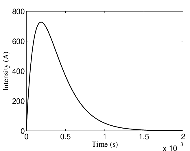
Refer to caption
Figure 5.4: Source current intensity (A) vs. time (s).

The axisymmetric problem has been solved by using a scalar formulation written in terms of the azimuthal component of a magnetic vector potential AθA_{\theta}. The corresponding weak formulation, although with boundary conditions different from those of our case, has been analyzed in [19], [20] with moving domains. In particular, the method was proved to converge with optimal order error estimates in terms of hh and Δ​t\Delta t under appropriate assumptions.

Refer to caption
Refer to caption
Figure 5.5: Coarsest mesh used for the 3D code (left) and mesh used by the axisymmetric code (right).

Figure 5.5 (right) shows the mesh used in the axisymmetric code. Concerning the 3D mesh, we have exploited the symmetry of the problem and solved it in 1/81/8 of the whole domain to reduce the number of degrees of freedom. The used mesh is shown in Figure 5.5 (left).

We have solved the problem with several successively refined meshes and a time-step conveniently reduced to analyze the convergence with respect to both, the mesh-size and the time-step simultaneously. Figure 5.6 shows a log-log plot of the relative error for the electric field, versus the number of degrees of freedom (d.o.f.). The curve shows that the obtained results converge to the ‘exact’ ones as hh and Δ​t\Delta t go to zero.

Refer to caption
Figure 5.6: 100×max1≤k≤M∥𝐄(tk)−𝐄kh∥L2(ΩC)3max1≤k≤M∥𝐄(tk)∥L2(ΩC)3100\times\frac{\underset{1\leq k\leq M}{\max}\|\mathbf{E}(t_{k})-\mathbf{E}^{k}_{h}\|_{\mathrm{L}^{2}(\Omega_{{}_{\mathrm{C}}\!})^{3}}}{\underset{1\leq k\leq M}{\max}\|\mathbf{E}(t_{k})\|_{\mathrm{L}^{2}(\Omega_{{}_{\mathrm{C}}\!})^{3}}} versus number of d.o.f. (log-log scale).

5.2.2 Input current model

As another application of our theoretical framework, we present the fully-discrete analysis for the input current model proposed in [18]. To this aim, we introduce the following Hilbert spaces

X\displaystyle X :={𝐰∈𝐇(𝐜𝐮𝐫𝐥;Ω):𝐰×𝒏=𝟎 on ΓC,𝐜𝐮𝐫𝐥𝐰⋅𝒏=𝟎 on ∂Ω},\displaystyle:=\left\{\mathbf{w}\in\mathbf{H}(\mathop{\mathbf{curl}}\nolimits;\Omega):\ \mathbf{w}\times\boldsymbol{n}=\boldsymbol{0}\textrm{ on }\Gamma_{{}_{\!\mathrm{C}}\!},\ \mathop{\mathbf{curl}}\nolimits\mathbf{w}\cdot\boldsymbol{n}=\boldsymbol{0}\textrm{ on }\partial\Omega\right\}, (5.11)
M\displaystyle M :={φ∈H1(ΩD):φ|ΓI1=0;φ|ΓIk=CI,k=2,…,MI}.\displaystyle:=\left\{\varphi\in\mathrm{H}^{1}(\Omega_{{}_{\mathrm{D}}\!}):\ \varphi|_{\Gamma_{{}_{\!\mathrm{I}}\!}^{1}}=0;\ \varphi|_{\Gamma_{{}_{\!\mathrm{I}}\!}^{k}}=C_{I},\ k=2,\ldots,M_{I}\right\}. (5.12)

with their usual norms in 𝐇(𝐜𝐮𝐫𝐥;Ω)\mathbf{H}(\mathop{\mathbf{curl}}\nolimits;\Omega) and H1(ΩD)\mathrm{H}^{1}(\Omega_{{}_{\mathrm{D}}\!}), respectively.

Let g∈L2​(0,T,L2​(Γ))g\in\mathrm{L}^{2}(0,T;\mathrm{L}^{2}(\Gamma)), In∈H2(0,T),n=1,⋯,NI_{n}\in\mathrm{H}^{2}(0,T),\,\,n=1,\cdots,N and 𝐇0∈𝐇(𝐜𝐮𝐫𝐥;Ω)\mathbf{H}_{0}\in\mathbf{H}(\mathop{\mathbf{curl}}\nolimits;\Omega) the initial magnetic field. We denote

⟨𝐟⁡(t),𝐯⟩=∫Ω𝐟⁡(t)⋅𝐯:=∑n=1NLn​(𝐯)​(In​(t)−In​(0))+∫Ω𝐜𝐮𝐫𝐥𝐇0⋅𝐯∀𝐯∈X,\left\langle\mathbf{f}(t),\mathbf{v}\right\rangle=\int_{\Omega}\mathbf{f}(t)\cdot\mathbf{v}:=\sum_{n=1}^{N}L_{n}(\mathbf{v})(I_{n}(t)-I_{n}(0))+\int_{\Omega}\mathop{\mathbf{curl}}\nolimits\mathbf{H}_{0}\cdot\mathbf{v}\quad\forall\mathbf{v}\in X,

for any t∈[0,T]t\in[0,T]. The variational formulation for the input current model (see [18]) is :

Problem 5.5.

Find 𝐮∈L2​(0,T,X)\mathbf{u}\in\mathrm{L}^{2}(0,T;X) and λ∈H1​(0,T,M)\lambda\in\mathrm{H}^{1}(0,T;M) such that

dd​t[∫ΩCσ𝐮(t)⋅𝐯+∫ΩDε𝐯⋅∇λ(t)]+∫Ω1μ𝐜𝐮𝐫𝐥𝐮(t)⋅𝐜𝐮𝐫𝐥𝐯=⟨𝐟(t),𝐯⟩\displaystyle\dfrac{d}{dt}\left[\int_{\Omega_{{}_{\mathrm{C}}\!}}\sigma\mathbf{u}(t)\cdot\mathbf{v}+\int_{\Omega_{{}_{\mathrm{D}}\!}}\varepsilon\mathbf{v}\cdot\nabla\lambda(t)\right]+\int_{\Omega}\frac{1}{\mu}\mathop{\mathbf{curl}}\nolimits\mathbf{u}(t)\cdot\mathop{\mathbf{curl}}\nolimits\mathbf{v}=\langle\mathbf{f}(t),\mathbf{v}\rangle ∀𝐯∈X,\displaystyle\forall\mathbf{v}\in X,
∫ΩDε𝐮(t)⋅∇μ=∫Γd(∫0tg(s)ds)μ\displaystyle\int_{\Omega_{{}_{\mathrm{D}}\!}}\varepsilon\mathbf{u}(t)\cdot\nabla\mu=\int_{\Gamma_{d}}\left(\int_{0}^{t}g(s)ds\right)\mu ∀μ∈M,\displaystyle\forall\mu\in M,
𝐮(⋅,0)=𝟎in ΩCand λ(0)=0in ΩD,\displaystyle\mathbf{u}(\cdot,0)=\boldsymbol{0}\quad\textrm{in }\Omega_{{}_{\mathrm{C}}\!}\quad\textrm{and }\quad\lambda(0)=0\quad\textrm{in }\Omega_{{}_{\mathrm{D}}\!},

where we have introduced the time primitive

λ(𝐱,t)=∫0tξ(𝐱,s)ds𝐱∈ΩD,t∈[0,T].\displaystyle\lambda(\mathbf{x},t)=\int_{0}^{t}\xi(\mathbf{x},s)ds\quad\mathbf{x}\in\Omega_{{}_{\mathrm{D}}\!}\,,\quad t\in[0,T].

of the original lagrange multiplier ξ\xi of the model in [18]. As before, to get the fully-discrete approximation for Problem 5.5, it is necessary to employ XhX_{h} and MhM_{h}, finite-dimensional subspaces of XX and MM, respectively. Thus, we define the following spaces

Xh:={𝐰∈𝒩h(Ω):𝐰×𝒏=𝟎onΓCand𝐜𝐮𝐫𝐥𝐰⋅𝒏=0on∂ΩD},\displaystyle X_{h}:=\left\{\mathbf{w}\in\mathcal{N}_{h}(\Omega):\,\,\mathbf{w}\times\boldsymbol{n}=\boldsymbol{0}\,\,\text{on}\,\,\Gamma_{{}_{\!\mathrm{C}}\!}\,\,\text{and}\,\,\mathop{\mathbf{curl}}\nolimits\mathbf{w}\cdot\boldsymbol{n}=0\,\,\text{on}\,\,\partial{\Omega_{{}_{\mathrm{D}}\!}}\right\},
Mh:={μ∈ℒ(ΩD):μ|ΓI1=0,μ|ΓIk=Ck,k=2,⋯,M},\displaystyle M_{h}:=\left\{\mu\in\mathcal{L}(\Omega_{{}_{\mathrm{D}}\!}):\,\,\mu|_{\Gamma_{{}_{\!\mathrm{I}}\!}^{1}}=0,\,\,\mu|_{\Gamma_{{}_{\!\mathrm{I}}\!}^{k}}=C_{k},\,\,\,k=2,\cdots,M\right\},

where 𝒩h​(Ω)\mathcal{N}_{h}(\Omega) and ℒ(ΩD)\mathcal{L}(\Omega_{{}_{\mathrm{D}}\!}) are Nédélec (see (5.5)) and Lagrange finite element spaces, respectively.

Problem 5.6.

Find 𝐮hn∈Xh\mathbf{u}_{h}^{n}\in X_{h} and λhn∈Mh\lambda_{h}^{n}\in M_{h} for n=1,⋯,Nn=1,\cdots,N such that

[∫ΩCσ𝐮hn−𝐮hn−1Δ​t⋅𝐯+∫ΩDε𝐯⋅∇λhn−∇λhn−1Δ​t]+∫Ω1μ𝐜𝐮𝐫𝐥𝐮hn⋅𝐜𝐮𝐫𝐥𝐯=∫Ω𝐟(tn)⋅𝐯∀𝐯∈Xh,\displaystyle\left[\int_{\Omega_{{}_{\mathrm{C}}\!}}\sigma\frac{\mathbf{u}_{h}^{n}-\mathbf{u}_{h}^{n-1}}{\Delta t}\cdot\mathbf{v}+\int_{\Omega_{{}_{\mathrm{D}}\!}}\varepsilon\mathbf{v}\cdot\frac{\nabla\lambda_{h}^{n}-\nabla\lambda_{h}^{n-1}}{\Delta t}\right]+\int_{\Omega}\frac{1}{\mu}\mathop{\mathbf{curl}}\nolimits\mathbf{u}_{h}^{n}\cdot\mathop{\mathbf{curl}}\nolimits\mathbf{v}=\int_{\Omega}\mathbf{f}(t_{n})\cdot\mathbf{v}\quad\forall\mathbf{v}\in X_{h},
∫ΩDε𝐮hn⋅∇μ=∫Γd(∫0tng(s)ds)μ∀μ∈Mh,\displaystyle\int_{\Omega_{{}_{\mathrm{D}}\!}}\varepsilon\mathbf{u}_{h}^{n}\cdot\nabla\mu=\int_{\Gamma_{d}}\left(\int_{0}^{t_{n}}g(s)ds\right)\mu\quad\forall\mu\in M_{h},
𝐮h0=𝟎in Ωand λh0=0in ΩD.\displaystyle\mathbf{u}_{h}^{0}=\boldsymbol{0}\quad\textrm{in }\Omega\quad\textrm{and }\quad\lambda_{h}^{0}=0\quad\textrm{in }\Omega_{{}_{\mathrm{D}}\!}.

Next, we deduce the existence and uniqueness of the fully-discrete solution of Problem 5.6. So, we will prove that the hypotheses H7-H8 hold. Consequently, we define the discrete kernel of bb given by

Vh={𝐯∈Xh:b⁡(𝐯,μ)=0​∀μ∈Mh}.\displaystyle V_{h}=\left\{\mathbf{v}\in X_{h}:\,b(\mathbf{v},\mu)=0\,\,\forall\mu\in M_{h}\right\}.

The proof of discrete inf-sup condition H7 is similar to the deduction of its continuous version (see [3, Theorem 3.2]). Then, we only show the proof of H8. To this end, we need to deduce a discrete version of [14, Proposition 7.4]. To do that, we introduce the following notation:

ℍ\displaystyle\mathbb{H} :=𝐇ΓI(𝐜𝐮𝐫𝐥𝟎;ΩD)∩𝐇ΓD(divε0;ΩD),\displaystyle:={\mathbf{H}}_{\Gamma_{{}_{\!\mathrm{I}}\!}}(\mathop{\mathbf{curl}}\nolimits^{\boldsymbol{0}};\Omega_{{}_{\mathrm{D}}\!})\cap{\mathbf{H}}_{\Gamma_{{}_{\!\mathrm{D}}\!}}(\mathop{\mathrm{div}}\nolimits^{0}_{\varepsilon};\Omega_{{}_{\mathrm{D}}\!}),
𝐇^ΓI(𝐜𝐮𝐫𝐥;ΩD)\displaystyle\widehat{\mathbf{H}}_{\Gamma_{{}_{\!\mathrm{I}}\!}}(\mathop{\mathbf{curl}}\nolimits;\Omega_{{}_{\mathrm{D}}\!}) :={𝐰∈𝐇ΓI(𝐜𝐮𝐫𝐥;ΩD):𝐜𝐮𝐫𝐥𝐰⋅𝒏=0 on ΓD},\displaystyle:=\left\{\mathbf{w}\in\mathbf{H}_{\Gamma_{{}_{\!\mathrm{I}}\!}}(\mathop{\mathbf{curl}}\nolimits;\Omega_{{}_{\mathrm{D}}\!}):\ \mathop{\mathbf{curl}}\nolimits\mathbf{w}\cdot\boldsymbol{n}=0\textrm{ on }\Gamma_{{}_{\!\mathrm{D}}\!}\right\},
H^(div;ΩD)\displaystyle\widehat{\mathrm{H}}(\mathop{\mathrm{div}}\nolimits;\Omega_{{}_{\mathrm{D}}\!}) :={𝐰∈H(div,ΩD):𝐰⋅𝒏|ΓD∈L2(ΓD)},\displaystyle:=\left\{\mathbf{w}\in\mathrm{H}(\mathop{\mathrm{div}}\nolimits,\Omega_{{}_{\mathrm{D}}\!}):\ \mathbf{w}\cdot\boldsymbol{n}|_{\Gamma_{{}_{\!\mathrm{D}}\!}}\in\mathrm{L}^{2}(\Gamma_{{}_{\!\mathrm{D}}\!})\right\},
𝒩(ΩD)\displaystyle\mathcal{N}(\Omega_{{}_{\mathrm{D}}\!}) :={𝐯|ΩD:𝐯∈𝒩(Ω)},\displaystyle:=\left\{\mathbf{v}|_{\Omega_{{}_{\mathrm{D}}\!}}:\mathbf{v}\in\mathcal{N}(\Omega)\right\},
𝒩(ΩC)\displaystyle\mathcal{N}(\Omega_{{}_{\mathrm{C}}\!}) :={𝐯|ΩC:𝐯∈𝒩(Ω)},\displaystyle:=\left\{\mathbf{v}|_{\Omega_{{}_{\mathrm{C}}\!}}:\mathbf{v}\in\mathcal{N}(\Omega)\right\},
Vh,D\displaystyle V_{h,\mathrm{D}} :={𝐰∈𝐇^ΓI(𝐜𝐮𝐫𝐥;ΩD)∩ℍ∩𝒩(ΩD):b(𝐰,φ)=0∀φ∈Mh}.\displaystyle:=\left\{\mathbf{w}\in\widehat{\mathbf{H}}_{\Gamma_{{}_{\!\mathrm{I}}\!}}(\mathop{\mathbf{curl}}\nolimits;\Omega_{{}_{\mathrm{D}}\!})\cap\mathbb{H}\cap\mathcal{N}(\Omega_{{}_{\mathrm{D}}\!}):\,\,b(\mathbf{w},\varphi)=0\quad\forall\varphi\in M_{h}\right\}.
Lemma 5.4.

There exist a constant C>0C>0 independent of hh such that

∥𝐯∥0,ΩD≤C∥𝐜𝐮𝐫𝐥𝐯∥0,ΩD∀𝐯∈Vh,D.\|\mathbf{v}\|_{0,\Omega_{{}_{\mathrm{D}}\!}}\leq C\|\mathop{\mathbf{curl}}\nolimits\mathbf{v}\|_{0,\Omega_{{}_{\mathrm{D}}\!}}\quad\forall\mathbf{v}\in V_{h,\mathrm{D}}.
Proof.

The proof is adapted from [7, Lemma 4.7]. The authors have done the case on the which the conductors do not go through the boundary of Ω\Omega. Let 𝐯∈Vh,D\mathbf{v}\in V_{h,\mathrm{D}}. In virtue of an orthogonal decomposition of L2(ΩD)3\mathrm{L}^{2}(\Omega_{{}_{\mathrm{D}}\!})^{3} (see [14, Proposition 6.4]) we can write 𝐯=𝐜𝐮𝐫𝐥𝐐+∇χ+𝐤\mathbf{v}=\mathop{\mathbf{curl}}\nolimits\mathbf{Q}+\mathop{\mathbf{\nabla}}\nolimits{\chi}+\mathbf{k} with

𝐐∈𝐇ΓD(𝐜𝐮𝐫𝐥;ΩD)∩𝐇ΓI(div0;ΩD)∩ℍ⟂,χ∈HΓI1(ΩD)and𝐤∈ℍ.\displaystyle\mathbf{Q}\in{\mathbf{H}}_{\Gamma_{{}_{\!\mathrm{D}}\!}}(\mathop{\mathbf{curl}}\nolimits;\Omega_{{}_{\mathrm{D}}\!})\cap{\mathbf{H}}_{\Gamma_{{}_{\!\mathrm{I}}\!}}(\mathop{\mathrm{div}}\nolimits^{0};\Omega_{{}_{\mathrm{D}}\!})\cap\mathbb{H}^{\perp},\quad\chi\in\mathrm{H}_{\Gamma_{{}_{\!\mathrm{I}}\!}}^{1}(\Omega_{{}_{\mathrm{D}}\!})\quad\text{and}\quad\mathbf{k}\in\mathbb{H}.

By substituting 𝐮=𝐜𝐮𝐫𝐥𝐐\mathbf{u}=\mathop{\mathbf{curl}}\nolimits\mathbf{Q}, it is easy verify the following 𝐜𝐮𝐫𝐥𝐮=𝐜𝐮𝐫𝐥𝐯\mathop{\mathbf{curl}}\nolimits\mathbf{u}=\mathop{\mathbf{curl}}\nolimits\mathbf{v} in ΩD\Omega_{{}_{\mathrm{D}}\!}, div𝐮=0\mathop{\mathrm{div}}\nolimits\mathbf{u}=0 in ΩD\Omega_{{}_{\mathrm{D}}\!}, 𝐮⋅𝒏=0\mathbf{u}\cdot\boldsymbol{n}=0 on ΓD{\Gamma_{{}_{\!\mathrm{D}}\!}} and 𝐮×𝒏=𝟎\mathbf{u}\times\boldsymbol{n}=\boldsymbol{0} on ΓI{\Gamma_{{}_{\!\mathrm{I}}\!}}. Then,

𝐮∈𝐇ΓI(𝐜𝐮𝐫𝐥;ΩD)∩𝐇ΓD(divε0;ΩD),\mathbf{u}\in\mathbf{H}_{\Gamma_{{}_{\!\mathrm{I}}\!}}(\mathop{\mathbf{curl}}\nolimits;\Omega_{{}_{\mathrm{D}}\!})\cap{\mathbf{H}}_{\Gamma_{{}_{\!\mathrm{D}}\!}}(\mathop{\mathrm{div}}\nolimits^{0}_{\varepsilon};\Omega_{{}_{\mathrm{D}}\!}),

and consequently 𝐮∈Hs(ΩD)\mathbf{u}\in\mathrm{H}^{s}(\Omega_{{}_{\mathrm{D}}\!}) for some s>1/2s>1/2 and there exists C>0C>0 such that

∥u∥s,ΩD≤C∥u∥𝐇(𝐜𝐮𝐫𝐥;ΩD).\|u\|_{s,\Omega_{{}_{\mathrm{D}}\!}}\leq C\|u\|_{\mathbf{H}(\mathop{\mathbf{curl}}\nolimits;\Omega_{{}_{\mathrm{D}}\!})}.

Moreover, since 𝐮∈ℍ⟂\mathbf{u}\in\mathbb{H}^{\perp} and by using [14, Proposition 7.4], we have

∥𝐮∥s,ΩD≤C∥𝐜𝐮𝐫𝐥𝐮∥0,ΩD.\displaystyle\|\mathbf{u}\|_{s,\Omega_{{}_{\mathrm{D}}\!}}\leq C\|\mathop{\mathbf{curl}}\nolimits\mathbf{u}\|_{0,\Omega_{{}_{\mathrm{D}}\!}}. (5.13)

Furthermore, thanks to that 𝐜𝐮𝐫𝐥𝐮=𝐜𝐮𝐫𝐥𝐯∈L∞(ΩD)3\mathop{\mathbf{curl}}\nolimits\mathbf{u}=\mathop{\mathbf{curl}}\nolimits\mathbf{v}\in\mathrm{L}^{\infty}(\Omega_{{}_{\mathrm{D}}\!})^{3} then we can define Πh𝐮∈𝒩h(ΩD)\Pi_{h}\mathbf{u}\in\mathcal{N}_{h}(\Omega_{{}_{\mathrm{D}}\!}). Note that there exists ϕh∈Mh\phi_{h}\in M_{h} such that ∇ϕh=Πh​(∇χ+𝐤)\mathop{\mathbf{\nabla}}\nolimits\phi_{h}=\Pi_{h}(\mathop{\mathbf{\nabla}}\nolimits\chi+\mathbf{k}), and hence

∥𝐯∥0,ΩD2≤∥𝐯∥0,ΩD∥Πh𝐮∥0,ΩD.\displaystyle\|\mathbf{v}\|_{0,\Omega_{{}_{\mathrm{D}}\!}}^{2}\leq\|\mathbf{v}\|_{0,\Omega_{{}_{\mathrm{D}}\!}}\|\Pi_{h}\mathbf{u}\|_{0,\Omega_{{}_{\mathrm{D}}\!}}. (5.14)

On the other hand, for all K∈𝒯hK\in\mathcal{T}_{h} con K⊂ΩDK\subset\Omega_{{}_{\mathrm{D}}\!}, we obtain

‖Π​𝐮−𝐮‖0,K\displaystyle\|\Pi\mathbf{u}-\mathbf{u}\|_{0,K} ≤C​hs​(‖𝐮‖s,K+‖𝐜𝐮𝐫𝐥𝐯‖s,K)\displaystyle\leq Ch^{s}\left(\|\mathbf{u}\|_{s,K}+\|\mathop{\mathbf{curl}}\nolimits\mathbf{v}\|_{s,K}\right)
≤C⁡(hs​‖𝐮‖s,K+‖𝐜𝐮𝐫𝐥𝐯‖0,K),\displaystyle\leq C\left(h^{s}\|\mathbf{u}\|_{s,K}+\|\mathop{\mathbf{curl}}\nolimits\mathbf{v}\|_{0,K}\right),

where we have used the local inverse estimate

‖𝐜𝐮𝐫𝐥𝐯‖s,K≤C​h−s​‖𝐜𝐮𝐫𝐥𝐯‖0,K.\displaystyle\|\mathop{\mathbf{curl}}\nolimits\mathbf{v}\|_{s,K}\leq Ch^{-s}\|\mathop{\mathbf{curl}}\nolimits\mathbf{v}\|_{0,K}.

By using (5.13) and triangular inequality, we have

∥Πh𝐮∥0,ΩD≤C∥𝐜𝐮𝐫𝐥𝐯∥0,ΩD\displaystyle\|\Pi_{h}\mathbf{u}\|_{0,\Omega_{{}_{\mathrm{D}}\!}}\leq C\|\mathop{\mathbf{curl}}\nolimits\mathbf{v}\|_{0,\Omega_{{}_{\mathrm{D}}\!}}

Finally, the Lemma follows from (5.14). ∎

Lemma 5.5.

If we define

Xh(Ωc):={𝐯∈𝒩(Ωc):𝐯×𝒏=𝟎onΓC}.X_{h}(\Omega_{c}):=\left\{\mathbf{v}\in\mathcal{N}(\Omega_{c}):\,\,\mathbf{v}\times\boldsymbol{n}=\boldsymbol{0}\quad\text{on}\quad\Gamma_{{}_{\!\mathrm{C}}\!}\right\}.

Then, the lineal mapping ℰh:XΓC,h(ΩC)→Vh\mathcal{E}_{h}:X_{\Gamma_{{}_{\!\mathrm{C}}\!},h}(\Omega_{{}_{\mathrm{C}}\!})\to V_{h} characterized by

(ℰh𝐯c)|ΩC=𝐯c∀𝐯c∈Xh(ΩC),∫ΩD(𝐜𝐮𝐫𝐥ℰh𝐯c)⋅𝐜𝐮𝐫𝐥𝐰D=0∀𝐯c∈Xh(ΩC)∀𝐰D∈Vh,d.\begin{split}&(\mathcal{E}_{h}\mathbf{v}_{\mathrm{c}})|_{\Omega_{{}_{\mathrm{C}}\!}}=\mathbf{v}_{\mathrm{c}}\qquad\forall\mathbf{v}_{\mathrm{c}}\in X_{h}(\Omega_{{}_{\mathrm{C}}\!}),\\ &\int_{\Omega_{{}_{\mathrm{D}}\!}}(\mathop{\mathbf{curl}}\nolimits\mathcal{E}_{h}\mathbf{v}_{\mathrm{c}})\cdot\mathop{\mathbf{curl}}\nolimits\mathbf{w}_{{}_{\mathrm{D}}\!}=0\qquad\forall\mathbf{v}_{\mathrm{c}}\in X_{h}(\Omega_{{}_{\mathrm{C}}\!})\quad\forall\mathbf{w}_{{}_{\mathrm{D}}\!}\in V_{h,d}.\end{split}

is well defined and bounded.

Proof.

Let us denote 𝜸τC:𝒩h(ΩC)→H−1/2(divτ;∂ΩC)\boldsymbol{\gamma}_{\tau}^{{}^{\mathrm{C}}\!}:\mathcal{N}_{h}(\Omega_{{}_{\mathrm{C}}\!})\to\mathrm{H}^{-1/2}(\mathop{\mathrm{div}}\nolimits_{\tau};\partial\Omega_{{}_{\mathrm{C}}\!}) and 𝜸τD:𝒩h(ΩD)→H−1/2(divτ;∂ΩD)\boldsymbol{\gamma}_{\tau}^{{}^{\mathrm{D}}\!}:\mathcal{N}_{h}(\Omega_{{}_{\mathrm{D}}\!})\to\mathrm{H}^{-1/2}(\mathop{\mathrm{div}}\nolimits_{\tau};\partial\Omega_{{}_{\mathrm{D}}\!}) by tangential traces on 𝐇(𝐜𝐮𝐫𝐥;ΩC)\mathbf{H}(\mathop{\mathbf{curl}}\nolimits;\Omega_{{}_{\mathrm{C}}\!}) and 𝐇(𝐜𝐮𝐫𝐥;ΩD)\mathbf{H}(\mathop{\mathbf{curl}}\nolimits;\Omega_{{}_{\mathrm{D}}\!}), respectively. It follows that linear operator 𝜼:Xh(ΩC)→H−1/2(divτ;∂ΩD)\boldsymbol{\eta}:X_{h}(\Omega_{{}_{\mathrm{C}}\!})\to\mathrm{H}^{-1/2}(\mathop{\mathrm{div}}\nolimits_{\tau};\partial\Omega_{{}_{\mathrm{D}}\!}) given by

𝜼⁡(𝐯c):={𝜸τC(𝐯c)|ΓIon ΓI,𝟎,on ΓD,\boldsymbol{\eta}(\mathbf{v}_{\!\mathrm{c}}):=\left\{\begin{array}[]{ll}\boldsymbol{\gamma}_{\tau}^{{}^{\mathrm{C}}\!}(\mathbf{v}_{\!\mathrm{c}})|_{\Gamma_{{}_{\!\mathrm{I}}\!}}&\textrm{on }\Gamma_{{}_{\!\mathrm{I}}\!},\\ \boldsymbol{0},&\textrm{on }\Gamma_{{}_{\!\mathrm{D}}\!},\end{array}\right.

is well defined. Moreover, we have

‖𝜼(𝐯c)‖H−1/2(divτ;∂ΩD)=‖𝜸τC(𝐯c)‖H−1/2(divτ;∂ΩC)≤C1‖𝐯c‖𝐇(𝐜𝐮𝐫𝐥;ΩC)∀𝐯c∈𝐇ΓC(𝐜𝐮𝐫𝐥;ΩC).\left\lVert\boldsymbol{\eta}(\mathbf{v}_{\!\mathrm{c}})\right\rVert_{\mathrm{H}^{-1/2}(\mathop{\mathrm{div}}\nolimits_{\tau};\partial\Omega_{{}_{\mathrm{D}}\!})}=\left\lVert\boldsymbol{\gamma}_{\tau}^{{}^{\mathrm{C}}\!}(\mathbf{v}_{\!\mathrm{c}})\right\rVert_{\mathrm{H}^{-1/2}(\mathop{\mathrm{div}}\nolimits_{\tau};\partial\Omega_{{}_{\mathrm{C}}\!})}\leq C_{1}\left\lVert\mathbf{v}_{\!\mathrm{c}}\right\rVert_{\mathbf{H}(\mathop{\mathbf{curl}}\nolimits;\Omega_{{}_{\mathrm{C}}\!})}\qquad\forall\mathbf{v}_{\!\mathrm{c}}\in\mathbf{H}_{\Gamma_{{}_{\!\mathrm{C}}\!}}(\mathop{\mathbf{curl}}\nolimits;\Omega_{{}_{\mathrm{C}}\!}).

After considering the continuous right inverse of tangential operator 𝜸τD\boldsymbol{\gamma}_{\tau}^{{}^{\mathrm{D}}\!}, we can define the continuous linear operator ℒh:Xh(ΩC)→𝒩(ΩD)\mathcal{L}_{h}:X_{h}(\Omega_{{}_{\mathrm{C}}\!})\to\mathcal{N}(\Omega_{{}_{\mathrm{D}}\!}) given by

ℒh(𝐯c):=(𝜸τD)−1(𝜼(𝐯c))∀𝐯c∈Xh(ΩC)\mathcal{L}_{h}(\mathbf{v}_{\!\mathrm{c}}):=(\boldsymbol{\gamma}_{\tau}^{{}^{\mathrm{D}}\!})^{-1}(\boldsymbol{\eta}(\mathbf{v}_{\!\mathrm{c}}))\quad\forall\mathbf{v}_{\!\mathrm{c}}\in X_{h}(\Omega_{{}_{\mathrm{C}}\!})

there holds

ℒh(𝐯c)×𝒏=𝟎onΓDandℒh(𝐯c)|ΓI×𝒏=𝐯c|ΓI×𝒏.\mathcal{L}_{h}(\mathbf{v}_{\mathrm{c}})\times\boldsymbol{n}=\boldsymbol{0}\quad\text{on}\quad\Gamma_{{}_{\!\mathrm{D}}\!}\quad\text{and}\quad\mathcal{L}_{h}(\mathbf{v}_{\mathrm{c}})|_{\Gamma_{{}_{\!\mathrm{I}}\!}}\times\boldsymbol{n}=\mathbf{v}_{\mathrm{c}}|_{\Gamma_{{}_{\!\mathrm{I}}\!}}\times\boldsymbol{n}.

By denoting Hh(ΩD):=𝐇^ΓI(𝐜𝐮𝐫𝐥;ΩD)∩ℍ⊥∩𝒩h(ΩD)\mathrm{H}_{h}(\Omega_{{}_{\mathrm{D}}\!}):=\widehat{\mathbf{H}}_{\Gamma_{{}_{\!\mathrm{I}}\!}}(\mathop{\mathbf{curl}}\nolimits;\Omega_{{}_{\mathrm{D}}\!})\cap\mathbb{H}^{\bot}\cap\mathcal{N}_{h}(\Omega_{{}_{\mathrm{D}}\!}), we consider the following mixed problem

Problem 5.7.

Find 𝐳D∈Hh(ΩD)\mathbf{z}_{{}_{\mathrm{D}}\!}\in{\mathrm{H}}_{h}(\Omega_{{}_{\mathrm{D}}\!}) and ρ∈Mh\rho\in{M}_{h} such that

∫ΩD𝐜𝐮𝐫𝐥𝐳D⋅𝐜𝐮𝐫𝐥𝐰D+b(𝐰D,ρ)=−∫ΩD𝐜𝐮𝐫𝐥(ℒh(𝐯c))⋅𝐜𝐮𝐫𝐥𝐰D∀𝐰∈Hh(ΩD)b(𝐳D,μ)=−b(ℒh(𝐯c),μ)∀μ∈Mh(ΩD).\begin{split}\int_{\Omega_{{}_{\mathrm{D}}\!}}\mathop{\mathbf{curl}}\nolimits\mathbf{z}_{{}_{\mathrm{D}}\!}\cdot\mathop{\mathbf{curl}}\nolimits\mathbf{w}_{{}_{\mathrm{D}}\!}+b(\mathbf{w}_{{}_{\mathrm{D}}\!},\rho)&=-\int_{\Omega_{{}_{\mathrm{D}}\!}}\mathop{\mathbf{curl}}\nolimits(\mathcal{L}_{h}(\mathbf{v}_{\mathrm{c}}))\cdot\mathop{\mathbf{curl}}\nolimits\mathbf{w}_{{}_{\mathrm{D}}\!}\qquad\forall\mathbf{w}\in\mathrm{H}_{h}(\Omega_{{}_{\mathrm{D}}\!})\\ b(\mathbf{z}_{{}_{\mathrm{D}}\!},\mu)&=-b(\mathcal{L}_{h}(\mathbf{v}_{\mathrm{c}}),\mu)\qquad\forall\mu\in{M}_{h}(\Omega_{{}_{\mathrm{D}}\!}).\end{split}

Now, we proceed to show that the previous problem is well-posedness. By using the Lemma 5.4 the bilinear form given by

(𝐯D,𝐰D)↦∫ΩD𝐜𝐮𝐫𝐥𝐯D⋅𝐜𝐮𝐫𝐥𝐰D,\displaystyle(\mathbf{v}_{{}_{\mathrm{D}}\!},\mathbf{w}_{{}_{\mathrm{D}}\!})\mapsto\int_{\Omega_{{}_{\mathrm{D}}\!}}\mathop{\mathbf{curl}}\nolimits\mathbf{v}_{{}_{\mathrm{D}}\!}\cdot\mathop{\mathbf{curl}}\nolimits\mathbf{w}_{{}_{\mathrm{D}}\!},

is coercive on Vh,dV_{h,d}. Furthermore, the discrete inf-sup conditions is satisfied. In fact: by noting grad(Mh)⊂Hh(ΩD)\textbf{grad}(M_{h})\subset{\mathrm{H}}_{h}(\Omega_{{}_{\mathrm{D}}\!}). Thus, we obtain

sup𝐯D∈Hh(ΩD)b(𝐯D,μ)‖𝐯D‖𝐇(𝐜𝐮𝐫𝐥;ΩD)≥b⁡(∇μ,μ)‖∇μ‖𝐇(𝐜𝐮𝐫𝐥;ΩD)=ε0‖∇μ‖L2(ΩD)3∀μ∈Mh.\begin{split}\sup_{\mathbf{v}_{{}_{\mathrm{D}}\!}\in{\mathrm{H}}_{h}(\Omega_{{}_{\mathrm{D}}\!})}\dfrac{b(\mathbf{v}_{{}_{\mathrm{D}}\!},\mu)}{\left\lVert\mathbf{v}_{{}_{\mathrm{D}}\!}\right\rVert_{\mathbf{H}(\mathop{\mathbf{curl}}\nolimits;\Omega_{{}_{\mathrm{D}}\!})}}&\geq\dfrac{b(\mathop{\mathbf{\nabla}}\nolimits\mu,\mu)}{\left\lVert\mathop{\mathbf{\nabla}}\nolimits\mu\right\rVert_{\mathbf{H}(\mathop{\mathbf{curl}}\nolimits;\Omega_{{}_{\mathrm{D}}\!})}}=\varepsilon_{0}\left\lVert\mathop{\mathbf{\nabla}}\nolimits\mu\right\rVert_{\mathrm{L}^{2}(\Omega_{{}_{\mathrm{D}}\!})^{3}}\quad\forall\mu\in M_{h}.\end{split}

It follows from the Babuska-Brezzi theory that the Problem 5.7 has a unique solution, which satisfies

‖𝐳D‖𝐇(𝐜𝐮𝐫𝐥;ΩD)≤C‖𝐯c‖𝐇(𝐜𝐮𝐫𝐥;ΩC)∀𝐯c∈Xh(ΩC).\left\lVert\mathbf{z}_{{}_{\mathrm{D}}\!}\right\rVert_{\mathbf{H}(\mathop{\mathbf{curl}}\nolimits;\Omega_{{}_{\mathrm{D}}\!})}\leq C\left\lVert\mathbf{v}_{\!\mathrm{c}}\right\rVert_{\mathbf{H}(\mathop{\mathbf{curl}}\nolimits;\Omega_{{}_{\mathrm{C}}\!})}\qquad\forall\mathbf{v}_{\mathrm{c}}\in X_{h}(\Omega_{{}_{\mathrm{C}}\!}).

Hence, we define

ℰh​𝐯c:={𝐯cin ΩC,𝐳D+ℒh𝐯cin ΩD,\mathcal{E}_{h}\mathbf{v}_{\mathrm{c}}:=\left\{\begin{array}[]{ll}\mathbf{v}_{\mathrm{c}}&\textrm{in }\Omega_{{}_{\mathrm{C}}\!},\\ \mathbf{z}_{{}_{\mathrm{D}}\!}+\mathcal{L}_{h}\mathbf{v}_{\mathrm{c}}&\textrm{in }\Omega_{{}_{\mathrm{D}}\!},\end{array}\right.

there holds

𝐯c|ΓI×𝒏=ℒh(𝐯c)|ΓI×𝒏and𝐳D|ΓI×𝒏=𝟎,\mathbf{v}_{\mathrm{c}}|_{\Gamma_{{}_{\!\mathrm{I}}\!}}\times\boldsymbol{n}=\mathcal{L}_{h}(\mathbf{v}_{\mathrm{c}})|_{\Gamma_{{}_{\!\mathrm{I}}\!}}\times\boldsymbol{n}\quad\text{and}\quad\mathbf{z}_{{}_{\mathrm{D}}\!}|_{\Gamma_{{}_{\!\mathrm{I}}\!}}\times\boldsymbol{n}=\boldsymbol{0},

from which the result follows. ∎

The following result may be proved in much the same way as Lemma 5.15. This is due to Lemma 5.4 and Lemma 5.5.

Lemma 5.6.

There exist positive constants γ^\widehat{\gamma} and α^\widehat{\alpha} such that

∫Ω1μ|𝐜𝐮𝐫𝐥𝐯|2+γ^∫ΩCσ|𝐯|2≥α^‖𝐯‖𝐇(𝐜𝐮𝐫𝐥;Ω)2∀𝐯∈Vh.\int_{\Omega}\dfrac{1}{\mu}|\mathop{\mathbf{curl}}\nolimits\mathbf{v}|^{2}+\widehat{\gamma}\int_{\Omega_{{}_{\mathrm{C}}\!}}\sigma|\mathbf{v}|^{2}\geq\widehat{\alpha}\left\lVert\mathbf{v}\right\rVert_{\mathbf{H}(\mathop{\mathbf{curl}}\nolimits;\Omega)}^{2}\qquad\forall\mathbf{v}\in V_{h}. (5.15)
Proof.

Let 𝐯∈Vh\mathbf{v}\in V_{h}, considering 𝐯c:=𝐯|ΩC\mathbf{v}_{\mathrm{c}}:=\mathbf{v}|_{\Omega_{{}_{\mathrm{C}}\!}} and ℰh​𝐯c\mathcal{E}_{h}\mathbf{v}_{\mathrm{c}} given by Lemma 5.5, we can define 𝐰~:=𝐯−ℰh​𝐯c\widetilde{\mathbf{w}}:=\mathbf{v}-\mathcal{E}_{h}\mathbf{v}_{\mathrm{c}}, then

𝐰~=𝟎 in ΩC,𝐰~∈Vh,𝐰~|ΩD∈Vh,d.\widetilde{\mathbf{w}}=\boldsymbol{0}\textrm{ in $\Omega_{{}_{\mathrm{C}}\!}$},\qquad\widetilde{\mathbf{w}}\in V_{h},\qquad\widetilde{\mathbf{w}}|_{\Omega_{{}_{\mathrm{D}}\!}}\in V_{h,d}.

Thus, by using the Lemma 5.4, the continuity of ℰh\mathcal{E}_{h} and proceeding as in Lemma 5.3, it is deduced the result. ∎

Consequently, we can use the results of Section 3 to conclude that the fully-discrete approximation of the Problem 5.3 has a unique solution (𝐮hn,λhn)∈Xh×Mh,n=1,…,N(\mathbf{u}_{h}^{n},\lambda_{h}^{n})\in X_{h}\times M_{h},\ n=1,\dots,N. Now, our next to goal is to obtain error fully-discrete scheme. Before, we recall that λ=0\lambda=0 (see [18, Theorem 2.4]). As in subsection 5.2.1 and by assuming 𝐮∈H1​(0,T,X)∩H2​(0,T,L2​(Ω)3)\mathbf{u}\in\mathrm{H}^{1}(0,T;X)\cap\mathrm{H}^{2}(0,T;\mathrm{L}^{2}(\Omega)^{3}) (see (5.11)), we can obtain similar results as in Theorem 5.3 and Theorem 5.5. These results allow us to obtain the asymptotic error estimates. In fact, fixing an index r>12r>\frac{1}{2} and considering 𝒳:=𝐇r(𝐜𝐮𝐫𝐥,Ω)∩X\mathcal{X}:=\mathbf{H}^{r}(\mathop{\mathbf{curl}}\nolimits,\Omega)\cap X (see (5.9)), according to [15, Lemma 2.2], the Nédélec interpolant operator Ih𝒩:𝒳→XhI_{h}^{\mathcal{N}}:\mathcal{X}\to X_{h} is well defined and we can easily obtain an analogous result to Corollary 5.2. Thus, we easily obtain similar error estimates to those that were given in Remark 5.6 for the approximation of the electric and magnetic field at each time step. Finally, for some numerical results of this subsection that confirm the theoretical result obtained in this work, we refer the reader to [18, Section 4].

Funding
This work was partially supported by Colciencias through the 727 call, University of Cauca through project VRI ID 5243 and by Universidad Nacional de Colombia through Hermes project 4633246332.

Availability of data and materials
Not applicable.

Competing interests
The authors declare that they have no competing interests.

Authors contributions
The authors declare that the work was realized in collaboration with the same responsibility. All authors read and approved the final manuscript.

References

  • [1] Acevedo, R., Meddahi, S. & Rodríguez, R.(2009) An 𝑬\boldsymbol{E}-based mixed formulation for a time-dependent eddy current problem. Mathematics of Computation, 78, 1929–1949.
  • [2] Acevedo, R. and Meddahi, S.(2011) An 𝑬\boldsymbol{E}-based mixed FEM and BEM coupling for a time-dependent eddy current problem. IMA Journal of Numerical Analysis, 31(2), 667–697.
  • [3] Acevedo, R. C. Gómez and López-Rodríguez, B. (2020) Well-posedness for a family of degenerate parabolic mixed equations. Submitted, arXiv preprint arXiv:3172886.
  • [4] Acevedo, R. Navia, P. and Alvarez, E. A boundary and finite element coupling for a magnetically nonlinear eddy current problem, Electronic Transactions on Numerical Analysis, 50, 2020, 230-248.
  • [5] Ammari, H. Buffa, A. and Nédélec, A. C. A justification of eddy currents model for the Maxwell equation, SIAM J. Appl. Math., 60, 2000, 1805–1823.
  • [6] Alonso Rodríguez & A. and Valli, A.(1999) An optimal domain decomposition preconditioner for low-frequency time-harmonic Maxwell equations Mathematics of Computation, 68, 607–631.
  • [7] Alonso-Rodríguez, A. & Valli, A.(2010) Eddy Current Approximation of Maxwell Equations: Theory, algorithms and applications, Springer
  • [8] Ammari, H. Buffa, A. & Nédélec, A. C(2000) A justification of eddy currents model for the Maxwell equation, SIAM J. Appl. Math., 60, 1805–1823.
  • [9] Bernardi, C. & Raugel, G.(1985) A conforming finite element method for the time-dependent Navier-Stokes equations, SIAM J. Numer. Anal., 22, 455–473.
  • [10] Boffi, D. & Gastaldi, L.(2004) Analysis of finite element approximation of evolution problems in mixed form, SIAM J. Numer. Anal., 42, 1502–1526.
  • [11] Amrouche, C. and Bernardi, C. and Dauge, M. & Girault, V.(1998) Vector potentials in three-dimensional non-smooth domains, Math. Methods Appl. Sci., 21, 823–864.
  • [12] J. Camaño, and R. Rodríguez, Analysis of a FEM-BEM model posed on the conducting domain for the time-dependent eddy current problem, J. Comput. Appl. Math., vol. 236, no. 13, pp. 3084–3100, 2012.
  • [13] Emson, C.R.I. and Simkin, J.,(1983) An optimal method for 3D eddy currents.. IEEE Trans. Magn 19 2450-2452.
  • [14] P. Fernandes and G. Gilardi,(1997) Magnetostatic and electrostatic problems in inhomogeneous anisotropic media with irregular boundary and mixed boundary conditions. Math. Models Meth. Appl. Sci. 7 957–991.
  • [15] Bermúdez, A., Rodríguez R. and Salgado, P.(2005) Numerical analysis of electric field formulations of the eddy current model. Numer. Math., 102 181–201.
  • [16] A. Bermúdez, B. López-Rodríguez, R. Rodríguez and P. Salgado(2012) , Numerical analysis of a penalty approach for the solution of a transient eddy current problem. Comput. Math Appl. 9 2503-2526.
  • [17] A. Bermúdez, B. López-Rodríguez, R. Rodríguez and P. Salgado(2012) , Numerical solution of transient eddy current problems with input current intensities as boundary data. IMA J. Numer. Anal. 32 1001–1029.
  • [18] Bermúdez, A., López-Rodríguez, B., Rodríguez, R. & Salgado, P.(2013) An eddy current problem in terms of a time-primitive of the electric field with non-local source conditions, ESAIM - Mathematical Modelling and Numerical Analysis, 47, 875–902.
  • [19] Bermúdez, A., Muñoz, R., Reales, C., Rodríguez, R. and Salgado, P.(2013) A transient eddy current problem on a moving domain. Mathematical analysis, SIAM Journal on Mathematical Analysis, 45, 3629–3650.
  • [20] Bermúdez, A., Muñoz, R., Reales, C., Rodríguez, R. and Salgado, P.(2016) A transient eddy current problem on a moving domain. Numerical analysis, Advances in Computational Mathematics, 42, 757–789.
  • [21] Bermúdez, A., Rodríguez, R. & Salgado, P.(2002) A finite element method with Lagrange multipliers for low-frequency harmonic Maxwell equations, SIAM J. Numer. Anal., 40, 1823–1849.
  • [22] Bossavit, A.(1998) Computational Electromagnetism, Academic Press Inc.
  • [23] Ciarlet, P.(2002) The Finite Element Method for Elliptic Problems, SIAM
  • [24] Ern, A. & Guermond, J.-L.(2004) Theory and Practice of Finite Elements, Spinger-Verlag
  • [25] Hiptmair. R(2002) Finite elements in computational electromagnetism, Numerica, 11, 2002, pp. 237–339.
  • [26] Johnson, C. & Thomée, V.(1981) Error estimates for some mixed finite element methods for parabolic type problems. RAIRO Anal. Numér., 15, 41–78.
  • [27] Panton R.  L. (2013) Incompressible Flow, Wiley, New York, 2013.
  • [28] Meddahi, S. & Selgas, V.(2003) A mixed-FEM and BEM coupling for a three-dimensional eddy current problem M2AN Math. Model. Numer. Anal., 37, 291–318
  • [29] Arnold, D.N., Brezzi, F. & Fortin, M.(1984) A stable finite element for the stokes equations, Calcolo, 21, 337-344
  • [30] Weiß\ss B. and Bíró O. (2004) On the convergence of trasient eddy-current problems. IEEE Trans. Magn 40 957–960.
  • [31] Zheng, W., Chen, Z. and Wang, L. (2006) An adaptive finite element method for the HH-ψ\psi formulation of time-dependent eddy current problems. Numer. Math. 103 667–689.