跳到论文正文
W Papers独立论文阅读器 arXiv:2009.02262 论文正文 计算阅读时间 · 0%
引用这篇论文根据当前论文元数据生成,正式投稿前建议核对。


License: arXiv.org perpetual non-exclusive license
arXiv:2009.02262v2 [econ.EM] 13 Dec 2021
Abstract

The environmental Kuznets curve predicts an inverted U-shaped relationship between environmental pollution and economic growth. Current analyses frequently employ models which restrict nonlinearities in the data to be explained by the economic growth variable only. We propose a Generalized Cointegrating Polynomial Regression (GCPR) to allow for an alternative source of nonlinearity. More specifically, the GCPR is a seemingly unrelated regression with (1) integer powers of deterministic and stochastic trends for the individual units, and (2) a common flexible global trend. We estimate this GCPR by nonlinear least squares and derive its asymptotic distribution. Endogeneity of the regressors will introduce nuisance parameters into the limiting distribution but a simulation-based approach nevertheless enables us to conduct valid inference. A multivariate subsampling KPSS test is proposed to verify the correct specification of the cointegrating relation. Our simulation study shows good performance of the simulated inference approach and subsampling KPSS test. We illustrate the GCPR approach using data for Austria, Belgium, Finland, the Netherlands, Switzerland, and the UK. A single global trend accurately captures all nonlinearities leading to a linear cointegrating relation between GDP and CO2 for all countries. This suggests that the environmental improvement of the last years is due to economic factors different from GDP.

JEL Classification: C12, C13, C32, O44, Q20

Keywords: Cointegration Testing, Environmental Kuznets Curve, Generalized Cointegrating Polynomial Regression, Power Law Trends

1 Introduction

On page 370 of their seminal paper, Grossman and Krueger 1995 conclude:

“Contrary to the alarmist cries of some environmental groups, we find no evidence that economic growth does unavoidable harm to the natural habitat. Instead we find that while increases in GDP may be associated with worsening environmental conditions in very poor countries, air and water quality appear to benefit from economic growth once some critical level of income has been reached.”

The quote above suggests an inverted U-shaped relationship between environmental degradation and economic growth. This relationship is currently known as the Environmental Kuznets Curve (EKC) and it forms an active research area. Its relevance becomes clear if we look at some forecasts of long-run economic growth. The projected GDP per capita growth of the world is about 2.1% per year for the next decades (chapter 3 in Nordhaus 2013; Gillingham and Nordhaus 2018) and this growth is partially powered by carbon-based energy resources, water usage, and material consumption. In absence of an EKC, economic growth will place more and more stress on the environment. Alternatively, if the EKC exists, then the inverted U-shape eventually implies a turning point after which economic growth and environmental improvement go hand in hand. Due to such considerations, there is now, some 25 years after its first conception, a rich literature that (1) reports on the experimental evidence on the existence/nonexistence of the EKC, (2) provides economic theory to explain the EKC, and/or (3) refines the econometric tools that are used to analyse the EKC.11 1 Further references to these specific areas of research can be found in the review articles by Dasgupta et al. 2002, Stern 2004, and Carson 2009 among others. To quantify the volume of the literature we have entered the search query “Environmental Kuznets Curve’’ into the Web of Science: more than 4,200 references are found.22 2 Web of Science, accessed on December 6, 2021, http://www.webofknowledge.com.

Driven by contradictory empirical results as well as the variability in estimated turning points, the EKC has been criticised on two main points. First, the income variable was initially treated as a stationary variable whereas later research shows that the unit root hypothesis often cannot be rejected (see Galeotti et al. 2009, p. 553; Stern 2017, p. 14–15). Nonstationarity has further implications because EKC regressions include higher integer powers of GDP as well. This combination of nonstationarity and nonlinearity places the EKC in the nonlinear cointegration literature and appropriate econometric techniques should be employed. Such techniques have been developed in Wagner 2015 and Wagner and Hong 2016 under the name of Cointegrating Polynomial Regressions (CPRs). CPRs contain deterministic variables, integrated processes, and their integer powers.33 3 Stypka et al. 2017 reiterate the need to model the income variable as nonstationary. It is less important to use an estimation procedure acknowledging the fact that several integer powers of the same integrated process appear as regressors. That is, Stypka et al. 2017 find that the “standard estimator” which treats higher order powers of the integrated regressor as additional I(1) variables has the same limiting distribution as the CPR estimator. Multivariate generalizations of CPRs, Seemingly Unrelated Cointegrating Polynomial Regressions (SUCPRs), are discussed in Wagner et al. 2020 and Lin and Reuvers 2020.

As a second point of critique, there is an ongoing debate on the model specification. Various functional forms can describe the relationship between national income and the pollution variable. The quadratic specification is widespread but cubic relationships (Harbaugh et al. 2002; Wagner 2015) and double-nonlinear transformation (Lin et al. 2020) are also in use. Various specification tests are helpful while deciding on the right parametric specification (Hong and Phillips 2010; Wang and Phillips 2012; Wang et al. 2018). Alternatively, one could resort to nonparametric estimation procedures altogether (Wang and Phillips 2009; Linton and Wang 2016). Whereas such modelling approaches do allow for a more flexible relationship, they also implicitly assume that nonlinear environmental effects are solely attributable to economic growth. Relevant variables are thus potentially missing from the model specification. Such omitted variables are a valid concern because advances in green technology, pollution policy, and environmental awareness, may all influence pollution levels. However, such data is typically available for short time spans only (and for that reason often excluded from the model). Time effects can control for time-variation in unobserved effects (Vollebergh et al. 2009).

Current developments on nonlinear cointegration emphasize the role of the nonstationary regressor yet pay less attention to time effects. Time effects are important. The small simulation exercise in Table 1 illustrates the point. Foreshadowing our proposed model, we consider a multivariate setting with a global nonlinear, smooth time trend. The global trend is omitted by the researcher and a quadratic EKC-specification is estimated: yi,t=τ1,i+τ2,i​t+ϕ1,i​xi,t+ϕ2,i​xi,t2+ui,ty_{i,t}=\tau_{1,i}+\tau_{2,i}t+\phi_{1,i}x_{i,t}+\phi_{2,i}x_{i,t}^{2}+u_{i,t} (i=1,…,3i=1,\ldots,3), where xi,tx_{i,t} and yi,ty_{i,t} are unit-specific variables measuring income and environmental pollution, respectively. We test H0:ϕ2,1=ϕ2,2=ϕ2,3=0H_{0}:\phi_{2,1}=\phi_{2,2}=\phi_{2,3}=0 because a significantly negative coefficient in front of xi,t2x_{i,t}^{2} is typically interpreted as evidence of an EKC.44 4 For the moment, we focus on the curvature parameter. Clearly, for an inverted U-shaped relationship the coefficient in front of the linear term should be positive. Panel (A) reveals exacerbated rejection frequency as curvature caused by the global deterministic trend is mistakenly interpreted as curvature caused by the income variable. In other words, negative and significant coefficients in front of squared GDP are possibly caused by omitted nonlinear deterministic trends rather than being indicative of an EKC. To be on the safe side, we recommend researchers to include a nonlinear trend component in their model specification. If unnecessary, then this is rather innocuous. Indeed, Panel (B) of Table 1 shows that significant results for nonlinear economic growth effects continue to be found with modest losses in statistical power.

Table 1: The rejection rate (in %\%) when testing H0:ϕ2,1=ϕ2,2=ϕ2,3=0H_{0}:\phi_{2,1}=\phi_{2,2}=\phi_{2,3}=0. (A) Falsely inflated rejections of H0:ϕ2,1=ϕ2,2=ϕ2,3=0H_{0}:\phi_{2,1}=\phi_{2,2}=\phi_{2,3}=0 when time effects are omitted. (B) Adding an additional global deterministic trend to the model specification hardly influences the power of the test H0:ϕ2,1=ϕ2,2=ϕ2,3=0H_{0}:\phi_{2,1}=\phi_{2,2}=\phi_{2,3}=0. That is, significant coefficients in front of xi,t2x_{i,t}^{2} remain significant after adding a redundant flexible global trend.
Panel (A): Omitted Global Trend Panel (B): Redundant Global Trend
DGP yi,t=τg​tθ+τ1,i+τ2,i​t+ϕ1,i​xi,t+ui,ty_{i,t}=\tau_{g}t^{\theta}+\tau_{1,i}+\tau_{2,i}t+\phi_{1,i}x_{i,t}+u_{i,t} yi,t=τ1,i+τ2,i​t+ϕ1,i​xi,t+ϕ2​xi,t2+ui,t\text{\small{$y_{i,t}$}}=\text{\small{$\tau_{1,i}+\tau_{2,i}t+\phi_{1,i}x_{i,t}$}}+\phi_{2}x_{i,t}^{2}+\text{\small{$u_{i,t}$}}
Model yi,t=τ1,i+τ2,i​t+ϕ1,i​xi,t+ϕ2,i​xi,t2+ui,ty_{i,t}=\tau_{1,i}+\tau_{2,i}t+\phi_{1,i}x_{i,t}+\phi_{2,i}x_{i,t}^{2}+u_{i,t} Correct Specification yi,t=τg​tθ+ τ1,i+τ2,i​t+ϕ1,i​xi,t+ϕ2,i​xi,t2+ui,t\text{ \small{$y_{i,t}$}}=\tau_{g}t^{\theta}+\text{ \small{$\tau_{1,i}+\tau_{2,i}t+\phi_{1,i}x_{i,t}+\phi_{2,i}x_{i,t}^{2}+u_{i,t}$}}
τg(×10−5)\tau_{g}\,(\times 10^{-5}) FM-SOLS FM-SUR ϕ2\phi_{2} SimNLS SimNLS
0 6.30 6.63 0 6.93 5.70
-0.5 13.27 12.77 -0.5 9.20 6.97
-1 30.07 27.50 -1 14.97 9.97
-1.5 46.23 41.57 -1.5 30.47 20.70
-2 56.60 50.30 -2 55.33 40.53
-2.5 64.50 56.00 -2.5 81.73 69.20
-3 68.60 57.57 -3 93.97 89.50
  • •

    Note 1: For illustrative purpose, we consider a stylised example in this introduction. The exact parametrisation is available in Section of the Supplementary Material. More elaborate simulation results based on the empirical application are reported as simulation DGP2 in Section 4.

  • •

    Note 2: FM-SOLS and FM-SUR are documented in Wagner et al. 2020. The results in Panel (B) are based on simulation-based inference, see Section 3.2.

The contributions of this paper are fourfold. First, we propose the Generalized Cointegrating Polynomial Regression (GCPR). This multivariate model features a global power law trend to capture time effects. Power law trends have been employed to model non-constant growth rates in technology indices (Duggal et al. 1999; Duggal et al. 2007) and production functions (Klein et al. 2004). Within the EKC context, this flexible trend can capture common time effects that are implicit in omitted variables. Alternatively, as in Li and Linton 2020, the reader can view the global flexible trend as an outside option (next to the income variable) to describe nonlinearities in the data. Limiting distributions for estimators in models with purely deterministic power law trends have been reported in Phillips 2007, Robinson 2012 and Gao et al. 2020. The presence of integrated variables requires an alternative asymptotic framework. Moreover, due to endogeneity, approaches assuming pre-determined integrated regressors (Park and Phillips 1999; Park and Phillips 2001; Chang et al. 2001) are inappropriate and we instead opt for a proof along the lines of Chan and Wang 2015. The resulting limiting distribution is non-standard because (1) the scaling matrix with convergence rates is non-diagonal and parameter dependent, and (2) second-order bias terms are present. Second, we propose a simulation-based approach to conduct inference. Monte Carlo simulations show clear benefits of this simulation-based approach in terms of size control compared to existing methods. Third, in the spirit of Choi and Saikkonen 2010, we report a multivariate KPSS-type test to verify the stationarity of the error process thus enabling researchers to avoid spurious results or misspecified cointegrating relations. Fourth and finally, in the empirical application, we investigate the EKC for Austria, Belgium, Finland, the Netherlands, Switzerland and the UK over the period 1870–2014. Nonparametric estimates and tests confirm that the global trend captures all nonlinearities in the data. Nonlinear effects in log per capita GDP (and thus also evidence for an EKC) are absent. Given such findings, we offer a clear recommendation to researchers to check whether their EKC conclusions are robust to the inclusion of power law trends.

This paper is organized as follows. Section 2 introduces the model and the estimation framework. Asymptotic properties of the estimators and parameter inference are discussed in Section 3. The Monte Carlo simulations in Section 4 compare asymptotic results to finite sample performance. An in depth discussion of the Environment Kuznets Curve can be found in Section 5. Section 6 concludes. The proofs of the main theorems are collected in the Appendix and further information is available in the Supplementary Material.

Finally, some words on notation. The integer part of the number a∈ℝ+a\in\mathbb{R}^{+} is denoted by [a][a]. For a vector 𝒙∈ℝn\bm{x}\in\mathbb{R}^{n}, its pp-norm is denoted by ‖𝒙‖p=(∑i=1n|xi|p)1/p\|\bm{x}\|_{p}=(\sum_{i=1}^{n}|x_{i}|^{p})^{1/p}. For a matrix 𝑨\bm{A}, say of dimension (n×mn\times m), the induced pp-norm is defined as ‖𝑨‖p=sup𝒙≠𝟎‖𝑨​𝒙‖p/‖𝒙‖p\|\bm{A}\|_{p}=\sup_{\bm{x}\neq\bm{0}}\|\bm{A}\bm{x}\|_{p}/\|\bm{x}\|_{p}. We will omit the subscripts whenever p=2p=2. The (n×n)(n\times n) identity matrix is denoted 𝑰n\bm{I}_{n} and ın\bm{\imath}_{n} signifies an nn-dimensional column vector with all entries equal to 1. The block-diagonal matrix diag⁡[𝑨1,…,𝑨n]\operatorname{diag}[\bm{A}_{1},\ldots,\bm{A}_{n}] stacks the matrices 𝑨1,…,𝑨n\bm{A}_{1},\ldots,\bm{A}_{n} along its diagonal. We omit the integration bounds whenever the integration interval is [0,1][0,1]. The symbol “=d\stackrel{{\scriptstyle d}}{{=}}” stands for equality in distribution, and “⟶p\longrightarrow_{p}” and “⟶d\longrightarrow_{d}” denote convergence in probability and in distribution. If convergence occurs conditionally on the sample, then we add a superscript “*” to the standard notation. The probabilistic Landau symbols are Op​(⋅)O_{p}(\cdot) and op​(⋅)o_{p}(\cdot). Finally, the generic constant CC can change from line to line.

2 The Model and NLS Estimation

Our model specification enriches the Seemingly Unrelated Cointegrating Polynomial Regressions (SUCPRs) from Wagner et al. 2020 with a flexible deterministic trend. That is, each individual series in the system is affected by specific deterministic variables and integrated regressors (and their integer powers) while a global flexible trend describes nonlinear behaviour that is prevalent across all series. The resulting Generalized Cointegrating Polynomial Regression (GCPR) is given by:

yi,t=τgtθ+τ1,i+τ2,it+∑j=1piϕj,ixi,tj+ui,t,i=1,…,N,t=1,…,T,y_{i,t}=\tau_{g}t^{\theta}+\tau_{1,i}+\tau_{2,i}t+\sum_{j=1}^{p_{i}}\phi_{j,i}x_{i,t}^{j}+u_{i,t},\qquad i=1,\ldots,N,\qquad t=1,\ldots,T, (2.1)

where θ∈Θ⁡(ε)\theta\in\Theta(\varepsilon) with Θ(ε)={θ∈[θL,θU]:|θ|>ϵ,|θ−1|>ϵ}\Theta(\varepsilon)=\left\{\theta\in[\theta_{L},\theta_{U}]:\penalty\ |\theta|>\epsilon,\,|\theta-1|>\epsilon\right\} and −1<θL≤θU<∞-1<\theta_{L}\leq\theta_{U}<\infty. Alternatively, we write yi,t=τg​tθ+𝒛i,t′​𝜷i+ui,ty_{i,t}=\tau_{g}t^{\theta}+\bm{z}_{i,t}^{\prime}\bm{\beta}_{i}+u_{i,t}, where 𝒛i,t=[1,t,xi,t,…,xi,tpi]′\bm{z}_{i,t}=\big[1,t,x_{i,t},\ldots,x_{i,t}^{p_{i}}\big]^{\prime} and 𝜷i=[τ1,i,τ2,i,ϕ1,i,…,ϕpi,i]′\bm{\beta}_{i}=\big[\tau_{1,i},\tau_{2,i},\phi_{1,i},\ldots,\phi_{p_{i},i}\big]^{\prime}. Finally, we stack all NN equations in (2.1) in matrix form to retrieve

𝒚t=τgtθıN+𝒁t′𝜷+𝒖t,t=1,…,T,\bm{y}_{t}=\tau_{g}t^{\theta}\bm{\imath}_{N}+\bm{Z}_{t}^{\prime}\bm{\beta}+\bm{u}_{t},\qquad t=1,\ldots,T, (2.2)

with 𝒚t=[y1,t,…,yN,t]′\bm{y}_{t}=\big[y_{1,t},\ldots,y_{N,t}\big]^{\prime}, 𝒁t=diag⁡[𝒛1,t,…,𝒛N,t]\bm{Z}_{t}=\operatorname{diag}\big[\bm{z}_{1,t},\ldots,\bm{z}_{N,t}\big], and the vector 𝜷=[𝜷1′,…,𝜷N′]′\bm{\beta}=\big[\bm{\beta}_{1}^{\prime},\ldots,\bm{\beta}_{N}^{\prime}\big]^{\prime} of length p=2​N+∑i=1Npip=2N+\sum_{i=1}^{N}p_{i} containing all local parameters.

We consider nonlinear least squares (NLS) estimators of the unknown parameters in (2.1). As such, we define the objective function QT​(θ,τg,𝜷)=12​∑t=1T‖𝒚t−τg​tθ​ıN−𝒁t′​𝜷‖2Q_{T}(\theta,\tau_{g},\bm{\beta})=\frac{1}{2}\sum_{t=1}^{T}\big\|\bm{y}_{t}-\tau_{g}t^{\theta}\bm{\imath}_{N}-\bm{Z}_{t}^{\prime}\bm{\beta}\big\|^{2} and compute

(θ^T,τ^g,T,𝜷^T)=arg​min(θ,τg,𝜷)∈Θ⁡(ε)×ℝ×ℝp⁡QT​(θ,τ,𝜷).\left(\,\widehat{\theta}_{T},\widehat{\tau}_{g,T},\widehat{\bm{\beta}}_{T}\right)=\operatornamewithlimits{arg\;min}_{(\theta,\,\tau_{g},\,\bm{\beta})\in\Theta(\varepsilon)\times\mathbb{R}\times\mathbb{R}^{p}}Q_{T}(\theta,\tau,\bm{\beta}). (2.3)

The optimization problem in (2.3) is easy to solve. For any given θ\theta, model (2.2) is linear-in-parameters and the minimizers for τg\tau_{g} and 𝜷\bm{\beta} can be found from an OLS regression by constructing 𝒁t′​(θ)=[tθ​ıN​𝒁t′]\bm{Z}_{t}^{\prime}(\theta)=\big[t^{\theta}\bm{\imath}_{N}\;\bm{Z}_{t}^{\prime}\big] and computing [τg​(θ)𝜷⁡(θ)]=(∑t=1T𝒁t​(θ)​𝒁t′​(θ))−1​(∑t=1T𝒁t​(θ)​𝒚t)\left[\begin{smallmatrix}\tau_{g}(\theta)\\ \bm{\beta}(\theta)\end{smallmatrix}\right]=\left(\sum_{t=1}^{T}\bm{Z}_{t}(\theta)\bm{Z}_{t}^{\prime}(\theta)\right)^{-1}\left(\sum_{t=1}^{T}\bm{Z}_{t}(\theta)\bm{y}_{t}\right). We subsequently minimize the concentrated criterion function Q~T​(θ)=QT​(θ,τg​(θ),𝜷⁡(θ))\widetilde{Q}_{T}(\theta)=Q_{T}\big(\theta,\tau_{g}(\theta),\bm{\beta}(\theta)\big) to obtain θ^T\widehat{\theta}_{T}. At last, we plug in θ^T\widehat{\theta}_{T} and recover τ^g,T\widehat{\tau}_{g,T} and 𝜷^T\widehat{\bm{\beta}}_{T} through a final OLS estimation.

Remark 1

Keeping the powers of xi,tx_{i,t} fixed allows us to test for their significance and thereby distinguish between nonlinearities caused by deterministic and stochastic trends. This is important for our empirical application on the Environmental Kuznets Curve, see Section 5. Hu et al. 2021 study a model with a flexible power of the integrated regressor. That is, these authors derive the limiting distribution of the NLS estimators for β\beta and γ\gamma when yt=β​|xt|γ+uty_{t}=\beta|x_{t}|^{\gamma}+u_{t} with β≠0\beta\neq 0.

Remark 2

The GCPR of (2.1) can be extended in several directions. First, integer powers of deterministic trends can be added as long as Θ⁡(ε)\Theta(\varepsilon) is adjusted accordingly (to avoid collinearity). Second, multiple explanatory variables can be included. Related to the EKC, the literature suggests examples such as: population density (Selden and Song 1994), trade openness (Jalil and Feridun 2011), energy prices (Al-Mulali and Ozturk 2016), and educational level (Maranzano et al. 2021). For nonstationary variables, conditions similar to those on {xi,t}\{x_{i,t}\} should be fulfilled (Assumption 2 below). Stationary variables should be strictly exogenous. Avoiding the elaborate notation which would otherwise arise, we focus on the baseline specification in (2.1).

3 Asymptotic Theory

We subsequently study the asymptotic properties of the NLS estimators. To this end we first collect all the unknown parameters in the vector 𝜸=[θ,τg,𝜷′]′\bm{\gamma}=\big[\theta,\tau_{g},\bm{\beta}^{\prime}\big]^{\prime}. This vector is assumed to be an element of the parameter space 𝚪=Θ⁡(ε)×ℝ1+p\bm{\Gamma}=\Theta(\varepsilon)\times\mathbb{R}^{1+p}. The true parameter vector is 𝜸0=[θ0,τg,0,𝜷0′]′\bm{\gamma}_{0}=\big[\theta_{0},\tau_{g,0},\bm{\beta}_{0}^{\prime}\big]^{\prime}.

Assumption 1

The global trend is relevant, i.e. τg,0≠0\tau_{g,0}\neq 0.

Assumption 2

Let 𝛇t=[ηt′,𝛆t′]′\bm{\zeta}_{t}=[\eta_{t}^{\prime},\bm{\varepsilon}_{t}^{\prime}]^{\prime} be a sequence of i.i.d. random vectors with 𝔼⁡(𝛇t)=𝟎\mathbb{E}(\bm{\zeta}_{t})=\bm{0}, 𝚺=𝔼⁡(𝛇t​𝛇t′)≻0\bm{\varSigma}=\mathbb{E}\big(\bm{\zeta}_{t}\bm{\zeta}_{t}^{\prime})\succ 0, and 𝔼​‖𝛇t‖2​q<∞\mathbb{E}\left\|\bm{\zeta}_{t}\right\|^{2q}<\infty for some q>2q>2.

  1. (a)

    ut=∑k=0∞ψk​ηt−ku_{t}=\sum_{k=0}^{\infty}\psi_{k}\eta_{t-k} with ∑k=1∞k​|ψk|<∞\sum_{k=1}^{\infty}k|\psi_{k}|<\infty.

  2. (b)

    𝒙t=∑s=1t𝒗s\bm{x}_{t}=\sum_{s=1}^{t}\bm{v}_{s}, where 𝒗t=∑k=0∞𝚿k​𝜺t−k\bm{v}_{t}=\sum_{k=0}^{\infty}\bm{\varPsi}_{k}\bm{\varepsilon}_{t-k} with ∑k=0∞‖𝚿k‖<∞\sum_{k=0}^{\infty}\|\bm{\varPsi}_{k}\|<\infty and det(∑k=0∞𝚿k)≠0\det\left(\sum_{k=0}^{\infty}\bm{\varPsi}_{k}\right)\neq 0.

The first assumption is needed to avoid identification issues. That is, if τg,0=0\tau_{g,0}=0, then θ\theta is not identified and the Davies problem arrises when testing H0:τi=0H_{0}:\tau_{i}=0 (see Davies 1977; Davies 1987). Such complications are not investigated here and this is further reflected in our model specification (2.1). That is, we consider flexible powers of the deterministic trends but fixed powers of the stochastic trends, hence allowing us to test zero restrictions on (elements of) 𝜷\bm{\beta}. This is of crucial importance in the EKC application while determining whether nonlinear effects in the economic growth variables (xi,tx_{i,t}) remain significant after nonlinear time trends have been added to the model. Assumption 1 has been relaxed in the literature albeit for different models. Baek et al. 2015 and Cho and Phillips 2018 study the asymptotic behaviour of a quasi-likelihood ratio test when Assumption 1 is violated and the conditional mean of the data contains strictly stationary regressors and a flexible time trend. Alternatively, one can use drifting parameter sequences with different identification strengths as in Andrews and Cheng 2012.

Assumption 2 excludes cointegration among elements of 𝒙t\bm{x}_{t} and defines this vector as the partial sum of a short memory process. The latter implies that 1T∑t=1[r​T][𝒖t𝒗t]⟶d𝑩(r)=[𝑩u​(r)𝑩v​(r)]\frac{1}{\sqrt{T}}\sum_{t=1}^{[rT]}\left[\begin{smallmatrix}\bm{u}_{t}\\ \bm{v}_{t}\end{smallmatrix}\right]\longrightarrow_{d}\bm{B}(r)=\left[\begin{smallmatrix}\bm{B}_{u}(r)\\ \bm{B}_{v}(r)\end{smallmatrix}\right] where 𝑩⁡(r)\bm{B}(r) denotes an 2​N2N-dimensional vector Brownian motion with covariance matrix 𝛀=[𝛀u​u𝛀u​v𝛀v​u𝛀v​v]\bm{\varOmega}=\left[\begin{smallmatrix}\bm{\varOmega}_{uu}&\bm{\varOmega}_{uv}\\ \bm{\varOmega}_{vu}&\bm{\varOmega}_{vv}\end{smallmatrix}\right]. The one-sided long-run covariance matrix 𝚫=∑h=0∞𝔼⁡([𝒖t​𝒖t+h𝒖t​𝒗t+h′𝒗t​𝒖t+h𝒗t​𝒗t+h′])=[𝚫u​u𝚫u​v𝚫v​u𝚫v​v]\bm{\varDelta}=\sum_{h=0}^{\infty}\mathbb{E}\left(\left[\begin{smallmatrix}\bm{u}_{t}\bm{u}_{t+h}&\bm{u}_{t}\bm{v}_{t+h}^{\prime}\\ \bm{v}_{t}\bm{u}_{t+h}&\bm{v}_{t}\bm{v}_{t+h}^{\prime}\end{smallmatrix}\right]\right)=\left[\begin{smallmatrix}\bm{\varDelta}_{uu}&\bm{\varDelta}_{uv}\\ \bm{\varDelta}_{vu}&\bm{\varDelta}_{vv}\end{smallmatrix}\right] is partitioned similarly. Subscripts refer to specific elements. For example, 𝑩vi\bm{B}_{v_{i}} and 𝚫vi​uj\bm{\varDelta}_{v_{i}u_{j}} denote the iith and (i,j)(i,j)th elements of 𝑩v\bm{B}_{v} and 𝚫v​u\bm{\varDelta}_{vu}, respectively.

A concise exposition of our results asks for additional notation. An enumeration of various definitions is presented below.

  1. (1)

    Introduce 𝑫(i),T=diag⁡[1,T,T1/2,T,…,Tpi/2]\bm{D}_{(i),T}=\operatorname{diag}\big[1,T,T^{1/2},T,\ldots,T^{p_{i}/2}\big] to scale the deterministic and stochastic trends within each equation. For the full system of equation, define 𝑫Z,T=diag⁡[𝑫(1),T,…,𝑫(N),T]\bm{D}_{Z,T}=\operatorname{diag}\left[\bm{D}_{(1),T},\ldots,\bm{D}_{(N),T}\right], 𝑫θ0,T=T​[Tθ0Tθ0𝑫Z,T]\bm{D}_{\theta_{0},T}=\sqrt{T}\left[\begin{smallmatrix}T^{\theta_{0}}&&\\ &T^{\theta_{0}}&\\ &&\bm{D}_{Z,T}\end{smallmatrix}\right] and 𝑳τg,0,T=[1−τg,0​ln⁡T01𝑰p]\bm{L}_{\tau_{g,0},T}=\left[\begin{smallmatrix}1&-\tau_{g,0}\ln{T}&\\ 0&1&\\ &&\bm{I}_{p}\end{smallmatrix}\right]. Finally, set 𝑮𝜸0,T=𝑫θ0,T​𝑳τg,0,T′−1\bm{G}_{\bm{\gamma}_{0},T}=\bm{D}_{\theta_{0},T}\bm{L}_{\tau_{g,0},T}^{\prime-1}.

  2. (2)

    Define 𝒋i​(r)=[1,r,Bvi​(r),Bvi2​(r),…,Bvipi​(r)]′\bm{j}_{i}(r)=\left[1,r,B_{v_{i}}(r),B_{v_{i}}^{2}(r),\ldots,B_{v_{i}}^{p_{i}}(r)\right]^{\prime}, 𝑱Z​(r)=diag⁡[𝒋1​(r),…,𝒋N​(r)]\bm{J}_{Z}(r)=\operatorname{diag}\left[\bm{j}_{1}(r),\ldots,\bm{j}_{N}(r)\right], and 𝑱⁡(r,𝜸0)=[τg,0​rθ0​ln⁡r​ıN,rθ0​ıN,𝑱Z′​(r)]′\bm{J}(r;\bm{\gamma}_{0})=\Big[\tau_{g,0}r^{\theta_{0}}\ln{r}\,\bm{\imath}_{N},r^{\theta_{0}}\bm{\imath}_{N},\bm{J}_{Z}^{\prime}(r)\Big]^{\prime}.

  3. (3)

    For the second-order bias terms, we define 𝒃i=[𝟎1×2,1,2​∫𝑩vi​(r)​𝑑r,…,pi​∫𝑩vipi−1​(r)​𝑑r]′\bm{b}_{i}=\Big[\bm{0}_{1\times 2},1,2\int\bm{B}_{v_{i}}(r)dr,\ldots,p_{i}\int\bm{B}_{v_{i}}^{p_{i}-1}(r)dr\Big]^{\prime} and 𝓑v​u=[𝟎1×2,𝒃1′​𝚫v1​u1,…,𝒃N′​𝚫vN​uN]′\bm{\mathcal{B}}_{vu}=\big[\bm{0}_{1\times 2},\bm{b}_{1}^{\prime}\bm{\varDelta}_{v_{1}u_{1}},\dots,\bm{b}_{N}^{\prime}\bm{\varDelta}_{v_{N}u_{N}}\big]^{\prime}.

Theorem 1

Under Assumptions 1-2, we have

𝑮𝜸0,T(𝜸^T−𝜸0)⟶d(∫𝑱(r;𝜸0)𝑱′(r;𝜸0)dr)−1(∫𝑱(r;𝜸0)d𝑩u(r)+𝓑v​u)=:𝓙(𝜸0),\bm{G}_{\bm{\gamma}_{0},T}\big(\widehat{\bm{\gamma}}_{T}-\bm{\gamma}_{0}\big)\longrightarrow_{d}\left(\int\bm{J}(r;\bm{\gamma}_{0})\bm{J}^{\prime}(r;\bm{\gamma}_{0})\penalty\ dr\right)^{-1}\left(\int\bm{J}(r;\bm{\gamma}_{0})\penalty\ d\bm{B}_{u}(r)+{\bm{\mathcal{B}}}_{vu}\right)=:{\bm{\mathcal{J}}}(\bm{\gamma}_{0}),

as T→∞T\rightarrow\infty and NN fixed.

The proof of Theorem 1 is closely related to the work by Chan and Wang 2015. These authors provide the asymptotic distribution of NLS estimators under a set of general conditions in univariate, nonstationary time series models (see their theorem 3.1). The results in Chan and Wang 2015 and Wang et al. 2018 suggest that Assumption 2 can be replaced by a long memory specification for Δ​𝒙t\Delta\bm{x}_{t}. However, long memory parameters will enter the limiting distribution and inference will be complicated further. We illustrate Theorem 1 with two examples. These examples highlight the two mathematical features that complicate parameter inference.

Example 1

We consider yt=τ​tθ+uty_{t}=\tau t^{\theta}+u_{t} with innovations satisfying Assumption 2. The limiting distribution of the parameter estimators depends solely on the mean square Riemann-Stieltjes integrals ∫τ0​rθ0​ln⁡(r)​d​Bu\int\tau_{0}r^{\theta_{0}}\ln(r)dB_{u} and ∫rθ0​d​Bu\int r^{\theta_{0}}dB_{u}, and is therefore normally distributed (e.g., section 2.3 in Tanaka 2017). We have

[Tθ0+120Tθ0+12​τ0​ln⁡(T)Tθ0+12][θ^T−θ0τ^T−τ0]⟶dN(𝟎,Ωu​u(2θ0+1)3[2​τ02−τ0​(2​θ0+1)−τ0​(2​θ0+1)(2​θ0+1)2]−1).\begin{bmatrix}T^{\theta_{0}+\frac{1}{2}}&0\\ T^{\theta_{0}+\frac{1}{2}}\tau_{0}\ln(T)&T^{\theta_{0}+\frac{1}{2}}\end{bmatrix}\begin{bmatrix}\,\widehat{\theta}_{T}-\theta_{0}\\ \,\widehat{\tau}_{T}-\tau_{0}\end{bmatrix}\longrightarrow_{d}\mathrm{N}\left(\bm{0},\Omega_{uu}(2\theta_{0}+1)^{3}\begin{bmatrix}2\tau_{0}^{2}&-\tau_{0}(2\theta_{0}+1)\\ -\tau_{0}(2\theta_{0}+1)&(2\theta_{0}+1)^{2}\end{bmatrix}^{-1}\right). (3.1)

The scaling matrix in the LHS of (3.1), [Tθ0+120Tθ0+12​τ0​ln⁡(T)Tθ0+12]\left[\begin{smallmatrix}T^{\theta_{0}+\frac{1}{2}}&0\\ T^{\theta_{0}+\frac{1}{2}}\tau_{0}\ln(T)&T^{\theta_{0}+\frac{1}{2}}\end{smallmatrix}\right], depends on θ0\theta_{0} and is non-diagonal. The dependence on θ0\theta_{0} is unavoidable but asymptotic results for the case of a diagonal scaling matrix are obtainable at the expense of a singular joint distribution. That is, noting that [Tθ0+1200Tθ0+12/ln⁡(T)]=[10−τ01/ln⁡(T)]​[Tθ0+120Tθ0+12​τ0​ln⁡(T)Tθ0+12]\left[\begin{smallmatrix}T^{\theta_{0}+\frac{1}{2}}&0\\ 0&T^{\theta_{0}+\frac{1}{2}}/\ln(T)\end{smallmatrix}\right]=\left[\begin{smallmatrix}1&0\\ -\tau_{0}&1/\ln(T)\end{smallmatrix}\right]\left[\begin{smallmatrix}T^{\theta_{0}+\frac{1}{2}}&0\\ T^{\theta_{0}+\frac{1}{2}}\tau_{0}\ln(T)&T^{\theta_{0}+\frac{1}{2}}\end{smallmatrix}\right] and since limT→∞[10−τ01/ln⁡(T)]=[10−τ00]\lim_{T\to\infty}\left[\begin{smallmatrix}1&0\\ -\tau_{0}&1/\ln(T)\end{smallmatrix}\right]=\left[\begin{smallmatrix}1&0\\ -\tau_{0}&0\end{smallmatrix}\right], the continuous mapping theorem implies [Tθ0+1200Tθ0+12/ln⁡(T)][θ^T−θ0τ^T−τ0]⟶d[1/τ0−1]×N(𝟎,Ωu​u(2θ0+1)3).\left[\begin{smallmatrix}T^{\theta_{0}+\frac{1}{2}}&0\\ 0&T^{\theta_{0}+\frac{1}{2}}/\ln(T)\end{smallmatrix}\right]\left[\begin{smallmatrix}\widehat{\theta}_{T}-\theta_{0}\\ \widehat{\tau}_{T}-\tau_{0}\end{smallmatrix}\right]\longrightarrow_{d}\left[\begin{smallmatrix}1/\tau_{0}\\ -1\end{smallmatrix}\right]\times\mathrm{N}\left(\bm{0},\Omega_{uu}(2\theta_{0}+1)^{3}\right). This limiting distribution coincides with the result in theorem 6.3 of Phillips 2007.

Example 2

If yt=τ​tθ+ϕ​xt+uty_{t}=\tau t^{\theta}+\phi x_{t}+u_{t}, then the limiting distribution of the NLS estimator is:

[Tθ0+12Tθ0+12​τ0​ln⁡(T)Tθ0+12T][θ^T−θ0τ^T−τ0ϕ^T−ϕ0]⟶d[∫(τ0​rθ0​ln⁡(r))2​𝑑r∫τ0​r2​θ0​ln⁡(r)​𝑑r∫τ0​rθ0​ln⁡(r)​Bv​𝑑r∫τ0​r2​θ0​ln⁡(r)​𝑑r∫r2​θ0​𝑑r∫rθ0​Bv​𝑑r∫τ0​rθ0​ln⁡(r)​Bv​𝑑r∫rθ0​Bv​𝑑r∫Bv2​𝑑r]−1×([∫τ0​rθ0​ln⁡(r)​d​Bu∫rθ0​d​Bu∫Bv​d​Bu]+[00Δv​u]).\begin{bmatrix}T^{\theta_{0}+\frac{1}{2}}\\ T^{\theta_{0}+\frac{1}{2}}\tau_{0}\ln(T)&T^{\theta_{0}+\frac{1}{2}}\\ &&T\end{bmatrix}\begin{bmatrix}\widehat{\theta}_{T}-\theta_{0}\\ \widehat{\tau}_{T}-\tau_{0}\\ \widehat{\phi}_{T}-\phi_{0}\end{bmatrix}\longrightarrow_{d}\begin{bmatrix}\int\big(\tau_{0}r^{\theta_{0}}\ln(r)\big)^{2}dr&\int\tau_{0}r^{2\theta_{0}}{\ln(r)}dr&\int\tau_{0}r^{\theta_{0}}\ln(r)B_{v}dr\\ \int\tau_{0}r^{2\theta_{0}}{\ln(r)}dr&\int r^{2\theta_{0}}dr&\int r^{\theta_{0}}B_{v}dr\\ \int\tau_{0}r^{\theta_{0}}\ln(r)B_{v}dr&\int r^{\theta_{0}}B_{v}dr&\int B_{v}^{2}dr\end{bmatrix}^{-1}\times\\ \left(\begin{bmatrix}\int\tau_{0}r^{\theta_{0}}\ln(r)dB_{u}\\ \int r^{\theta_{0}}dB_{u}\\ \int B_{v}dB_{u}\end{bmatrix}+\begin{bmatrix}0\\ 0\\ \Delta_{vu}\end{bmatrix}\right).

This limiting distribution exhibits second order bias when Δv​u≠0\Delta_{vu}\neq 0, or when BuB_{u} and BvB_{v} are correlated.

Two features of the limiting distribution of 𝑮𝜸0,T​(𝜸^T−𝜸0)\bm{G}_{\bm{\gamma}_{0},T}\big(\widehat{\bm{\gamma}}_{T}-\bm{\gamma}_{0}\big) deserve further comments. First, as emphasised in Examples 1–2, the scaling matrix 𝑮𝜸0,T\bm{G}_{\bm{\gamma}_{0},T} features two less common properties: (1) this matrix depends on the true parameters 𝝉g,0\bm{\tau}_{g,0} and θ0\theta_{0}, and (2) 𝑮𝜸0,T\bm{G}_{\bm{\gamma}_{0},T} is not diagonal. These peculiarities are caused by the nonlinearity and nonstationarity of the model. More specifically, these features can be traced back to the presence of the global trend. Limiting distributions with a similar mathematical structure can be found in the structural breaks literature, cf. model setting II.b of Perron and Zhu 2005 and its detailed analysis in Beutner et al. 2020.

Second, the nonstationary regressor xi,tx_{i,t} enters the model (2.1) through a polynomial transformation of the form g⁡(xi,t,ϕi)=ϕi,1​xi,t+…+ϕi,pi​xi,tpig(x_{i,t},\bm{\phi}_{i})=\phi_{i,1}x_{i,t}+\ldots+\phi_{i,p_{i}}x_{i,t}^{p_{i}} (i=1,2,…,Ni=1,2,\ldots,N). In the terminology of Park and Phillips 2001 this part of the regression function is a linear combination of H0H_{0}-regular functions. It is well-documented in the literature, e.g. Chang et al. 2001 and Chan and Wang 2015, that this leads to second-order bias terms and hence nonstandard inference (except for the special case of strictly exogenous nonstationary regressors).

3.1 Consistent Long-Run Covariance Matrix Estimation

Correcting for second-order bias terms typically involves estimating long-run variance (LRV) matrices. This subsection establishes that the NLS residuals can be used to construct consistent kernel estimators for the LRV matrices 𝚫\bm{\varDelta} and 𝛀\bm{\varOmega}. Defining 𝑽t​(𝜸)=[𝒖t​(𝜸)′,Δ​𝒙t′]′\bm{V}_{t}(\bm{\gamma})=\big[\bm{u}_{t}(\bm{\gamma})^{\prime},\Delta\bm{x}_{t}^{\prime}]^{\prime} with 𝒖t​(𝜸)=𝒚t−τg​tθ​𝜾N−𝒁t′​𝜷\bm{u}_{t}(\bm{\gamma})=\bm{y}_{t}-\tau_{g}t^{\theta}\bm{\iota}_{N}-\bm{Z}_{t}^{\prime}\bm{\beta}, these LRV estimators are defined as

𝚫^T=1T​∑t=1T∑s=1tk⁡(|t−s|bT)​𝑽t​(𝜸^T)​𝑽t​(𝜸^T)′,𝛀^T=1T​∑t=1T∑s=1Tk⁡(|t−s|bT)​𝑽t​(𝜸^T)​𝑽t​(𝜸^T)′,\widehat{\bm{\varDelta}}_{T}=\frac{1}{T}\sum_{t=1}^{T}\sum_{s=1}^{t}k\left(\frac{|t-s|}{b_{T}}\right)\bm{V}_{t}(\,\widehat{\bm{\gamma}}_{T})\bm{V}_{t}(\,\widehat{\bm{\gamma}}_{T})^{\prime},\qquad\widehat{\bm{\varOmega}}_{T}=\frac{1}{T}\sum_{t=1}^{T}\sum_{s=1}^{T}k\left(\frac{|t-s|}{b_{T}}\right)\bm{V}_{t}(\,\widehat{\bm{\gamma}}_{T})\bm{V}_{t}(\,\widehat{\bm{\gamma}}_{T})^{\prime}, (3.2)

for some kernel function k⁡(⋅)k(\cdot) and bandwidth parameter bTb_{T}. The first NN elements of 𝑽t​(𝜸^T)\bm{V}_{t}(\,\widehat{\bm{\gamma}}_{T}) are the elements of the residual vector 𝒖^t=𝒚t−τ^g,T​tθ^T​ıN−𝒁t′​𝜷^T\widehat{\bm{u}}_{t}=\bm{y}_{t}-\widehat{\tau}_{g,T}\,t^{\widehat{\theta}_{T}}\bm{\imath}_{N}-\bm{Z}_{t}^{\prime}\widehat{\bm{\beta}}_{T}. The remaining elements are Δ​𝒙t=𝒗t\Delta\bm{x}_{t}=\bm{v}_{t}.

Assumption 3
  1. (a)

    k⁡(0)=1k(0)=1, k⁡(⋅)k(\cdot) is continuous at zero, and supx≥0|k⁡(x)|<∞\sup_{x\geq 0}\left|k(x)\right|<\infty.

  2. (b)

    ∫0∞k¯​(x)​𝑑x<∞\int_{0}^{\infty}\bar{k}(x)dx<\infty, where k¯​(x)=supy≥x|k⁡(y)|\bar{k}(x)=\sup_{y\geq x}\left|k(y)\right|.

  3. (c)

    The bandwidth parameters {bT:T≥1}\{b_{T}:T\geq 1\} satisfies {bT}⊆(0,∞)\{b_{T}\}\subseteq(0,\infty) and limT→∞(bT−1+T−1/2bTlnT)=0\lim_{T\to\infty}\left(b_{T}^{-1}+T^{-1/2}b_{T}\ln T\right)=0.

The conditions on the kernel function k⁡(⋅)k(\cdot), Assumptions 3(a)–(b), are identical to those in Jansson 2002. Jansson 2002 remarks that these assumptions “would appear to be satisfied by any kernel in actual use”. Commonly used kernel functions such as the Bartlett, Parzen, and Quadratic Spectral kernels indeed satisfy all these assumptions. Assumption 3(c) differs from the usual requirement, limT→∞(bT−1+T−1/2bT)=0\lim_{T\to\infty}\left(b_{T}^{-1}+T^{-1/2}b_{T}\right)=0, by a factor ln⁡T\ln T. The difference is caused by the estimation error in θ^T\widehat{\theta}_{T}. This error causes the residuals {𝒖^t}\{\widehat{\bm{u}}_{t}\} to be less close to the innovations {𝒖t}\{\bm{u}_{t}\} and we balance this by including autocovariance matrices of higher lags at a slower pace.

Theorem 2

Under Assumptions 1-3, we have 𝚫^T⟶p𝚫\widehat{\bm{\varDelta}}_{T}\longrightarrow_{p}\bm{\varDelta} and 𝛀^T⟶p𝛀\widehat{\bm{\varOmega}}_{T}\longrightarrow_{p}\bm{\varOmega}.

3.2 Simulation-Based Inference

The limiting distribution in Theorem 1 is nonpivotal and thus not directly suited for inference. Some popular solutions for linear-in-parameters cointegration models are: Saikkonen 1992’s (Saikkonen 1992) dynamic least squares, the integrated modified OLS and fixed-bb approaches by Vogelsang and Wagner 2014, and the fully modified approach advocated in Phillips and Hansen 1990 and Phillips 1995. For a nonlinear-in-parameter model as in (2.1), a preliminary Monte Carlo exercise55 5 The details are available in Section S5 of the Supplementary Material. The analytical results in that appendix also suggest that the convergence speed of θ^T\widehat{\theta}_{T} to θ\theta is too slow to recover the standard zero-mean Gaussian limiting distribution. shows poor performance for fully modified inference but promising results for a simulation based approach. We pursue the latter method for the remainder of this paper.

The main idea behind the simulation based approach is to replace nuisance parameters by consistent estimates and to rely on Monte Carlo (MC) simulations to approximate the limiting distribution. The empirical quantiles of these MC draws allow us to conduct inference. Clearly, this kind of approach will provide exact inference when the limiting distribution is invariant with respect to the nuisance parameters (e.g. Dufour and Khalaf 2002 and Dufour 2006). In the absence of such invariance, Wang et al. 2018 and Bergamelli et al. 2019 show that the simulation approach remains asymptotically justified in several model specification. We adapt the algorithm from Wang et al. 2018 to the current setting and prove its asymptotic validity.

Algorithm 1 (Simulation-Based Inference)
  1. Step 1:

    Estimate 𝜸^T\widehat{\bm{\gamma}}_{T} and use the residuals {𝒖^t}\{\widehat{\bm{u}}_{t}\} to compute the estimators 𝚫^T\widehat{\bm{\varDelta}}_{T} and 𝛀^T\widehat{\bm{\varOmega}}_{T} from (3.2).

  2. Step 2:

    Repeat for j=1,…,Jj=1,\ldots,J,

  1. (a)

    Draw random variables {𝒆t}t=1MT\{\bm{e}_{t}\}_{t=1}^{M_{T}} i.i.d. from N⁡(𝟎,𝑰2​N)\mathrm{N}(\bm{0},\bm{I}_{2N}).

  2. (b)

    Compute [𝝁^t𝒗^t]=𝛀^T1/2​𝒆t\left[\begin{smallmatrix}\widehat{\bm{\mu}}_{t}\\ \widehat{\bm{v}}_{t}\end{smallmatrix}\right]=\widehat{\bm{\varOmega}}_{T}^{1/2}\bm{e}_{t} and the partial sum 𝝌^t=[χ^1,t,…,χ^N,t]′=∑s=1t𝝊^s\widehat{\bm{\chi}}_{t}=\big[\widehat{\chi}_{1,t},\ldots,\widehat{\chi}_{N,t}\big]^{\prime}=\sum_{s=1}^{t}\widehat{\bm{\upsilon}}_{s}.

  3. (c)

    Let 𝑱^​(t,𝜸^T)=[τ^g,T​tθ^T​ln⁡t​ıN,tθ^T​ıN,𝒵^t′]′\widehat{\bm{J}}\big(t;\widehat{\bm{\gamma}}_{T}\big)=\Big[\,\widehat{\tau}_{g,T}\,t^{\widehat{\theta}_{T}}\ln{t}\,\bm{\imath}_{N},t^{\widehat{\theta}_{T}}\bm{\imath}_{N},\widehat{\mathcal{Z}}_{t}^{\prime}\Big]^{\prime}, where 𝒵^t=diag⁡[𝒛^1,t,…,𝒛^N,t]\widehat{\mathcal{Z}}_{t}=\operatorname{diag}\big[\widehat{\bm{z}}_{1,t},\ldots,\widehat{\bm{z}}_{N,t}\big] with 𝒛^i,t=[1,t,χ^i,t,…,χ^i,tpi]′\widehat{\bm{z}}_{i,t}=\Big[1,t,\widehat{\chi}_{i,t},\ldots,\widehat{\chi}_{i,t}^{\,p_{i}}\Big]^{\prime} (for i=1,…,Ni=1,\ldots,N). For a given MTM_{T}, construct the jjth simulated draw as

    𝓙^(j)​(𝜸^T,𝛀^T,𝚫^v​u−)={𝑮𝜸^T,MT′−1​[∑t=1MT𝑱^​(t,𝜸^T)​𝑱^​(t,𝜸^T)′]​𝑮𝜸^T,MT−1}−1​{𝑮𝜸^T,MT′−1​[∑t=1MT𝑱^​(t,𝜸^T)​𝝁^t]+𝓑^v​u−},\widehat{{\bm{\mathcal{J}}}}^{(j)}\left(\widehat{\bm{\gamma}}_{T},\widehat{\bm{\varOmega}}_{T},\widehat{\bm{\varDelta}}_{vu}^{-}\right)=\left\{\text{\footnotesize$\bm{G}_{\widehat{\bm{\gamma}}_{T},M_{T}}^{\prime-1}\left[\sum_{t=1}^{M_{T}}\widehat{\bm{J}}\big(t;\widehat{\bm{\gamma}}_{T}\big)\widehat{\bm{J}}\big(t;\widehat{\bm{\gamma}}_{T}\big)^{\prime}\right]\bm{G}_{\widehat{\bm{\gamma}}_{T},M_{T}}^{-1}$}\right\}^{-1}\left\{\text{\footnotesize$\bm{G}_{\widehat{\bm{\gamma}}_{T},M_{T}}^{\prime-1}\left[\sum_{t=1}^{M_{T}}\widehat{\bm{J}}\big(t;\widehat{\bm{\gamma}}_{T}\big)\,\widehat{\bm{\mu}}_{t}\right]+\widehat{\bm{\mathcal{B}}}_{vu}^{-}$}\right\},

    where 𝚫^v​u−\widehat{\bm{\varDelta}}_{vu}^{-} is a consistent estimator of the lower-left subblock of 𝚫−=[𝚫u​u−𝚫u​v−𝚫v​u−𝚫v​v−]=𝚺−𝚫′\bm{\varDelta}^{-}=\left[\begin{smallmatrix}\bm{\varDelta}_{uu}^{-}&\bm{\varDelta}_{uv}^{-}\\ \bm{\varDelta}_{vu}^{-}&\bm{\varDelta}_{vv}^{-}\end{smallmatrix}\right]=\bm{\varSigma}-\bm{\varDelta}^{\prime}, and 𝓑^v​u−=[𝟎1×2,𝒃^1′​𝚫^v1​u1−,…,𝒃^N′​𝚫^vN​uN−]′\widehat{\bm{\mathcal{B}}}_{vu}^{-}=\left[\bm{0}_{1\times 2},\widehat{\bm{b}}_{1}^{\prime}\widehat{\bm{\varDelta}}_{v_{1}u_{1}}^{-},\dots,\widehat{\bm{b}}_{N}^{\prime}\widehat{\bm{\varDelta}}_{v_{N}u_{N}}^{-}\right]^{\prime} with 𝒃^i=[𝟎1×2,1,2​1MT​∑t=1MT(χ^i,tMT),…,pi​1MT​∑t=1MT(χ^i,tMT)pi−1]′\widehat{\bm{b}}_{i}=\Bigg[\bm{0}_{1\times 2},1,2\frac{1}{M_{T}}\sum_{t=1}^{M_{T}}\Big(\frac{\widehat{\chi}_{i,t}}{\sqrt{M_{T}}}\Big),\ldots,p_{i}\frac{1}{M_{T}}\sum_{t=1}^{M_{T}}\Big(\frac{\widehat{\chi}_{i,t}}{\sqrt{M_{T}}}\Big)^{p_{i}-1}\Bigg]^{\prime}.

  1. Step 3:

    Use the empirical quantiles of elements of {𝓙^(1),…,𝓙^(J)}\left\{\widehat{{\bm{\mathcal{J}}}}^{(1)},\ldots,\widehat{{\bm{\mathcal{J}}}}^{(J)}\right\} to conduct inference.

Algorithm 1 uses a discretisation in MTM_{T} steps to approximate the limiting distribution of the parameters. In practice, and in accordance with Theorem 3, we can take MT=TM_{T}=T. Remark 3 details how simulation-based inference can be used to test hypotheses concerning the model’s parameters. Discussions on size and power are also presented there.

Theorem 3

Suppose Assumptions 1-3 hold, let {MT}⊆(0,∞)\{M_{T}\}\subseteq(0,\infty) with limT→∞MTT≤κ\lim_{T\to\infty}\frac{M_{T}}{T}\leq\kappa, for some κ<∞\kappa<\infty, then we have

{𝑮𝜸^T,T′−1​[∑t=1MT𝑱^​(t,𝜸^T)​𝑱^​(t,𝜸^T)′]​𝑮𝜸^T,T−1}−1​{𝑮𝜸^T,T′−1​[∑t=1MT𝑱^​(t,𝜸^T)​𝝁^t]+𝓑^v​u−}\displaystyle\left\{\bm{G}_{\widehat{\bm{\gamma}}_{T},T}^{\prime-1}\left[\sum_{t=1}^{M_{T}}\widehat{\bm{J}}\big(t;\widehat{\bm{\gamma}}_{T}\big)\widehat{\bm{J}}\big(t;\widehat{\bm{\gamma}}_{T}\big)^{\prime}\right]\bm{G}_{\widehat{\bm{\gamma}}_{T},T}^{-1}\right\}^{-1}\left\{\bm{G}_{\widehat{\bm{\gamma}}_{T},T}^{\prime-1}\left[\sum_{t=1}^{M_{T}}\widehat{\bm{J}}\big(t;\widehat{\bm{\gamma}}_{T}\big)\,\widehat{\bm{\mu}}_{t}\right]+\widehat{\bm{\mathcal{B}}}_{vu}^{-}\right\} (3.3)
⟶d∗(∫𝑱(r;𝜸0)𝑱(r;𝜸0)′dr)−1(∫𝑱(r;𝜸0)d𝑩u(r)+𝓑v​u),\displaystyle\longrightarrow_{d^{*}}\left(\int\bm{J}(r;\bm{\gamma}_{0})\bm{J}(r;\bm{\gamma}_{0})^{\prime}\penalty\ dr\right)^{-1}\left(\int\bm{J}(r;\bm{\gamma}_{0})\penalty\ d\bm{B}_{u}(r)+{\bm{\mathcal{B}}}_{vu}\right),

in probability.

Theorem 3 establishes the asymptotic validity of the simulation approach. That is, for a large enough JJ, the empirical quantiles of the simulated distribution will coincide with the asymptotic distribution. Two remarks are important. First, even though the simulation algorithm is adapted from Wang et al. 2018, the proof of Theorem 3 is not. In particular, the method of proof is similar to Theorem 1 and continues to allow for endogeneity of the regressors. Second, the simulation approach mimics the stochastic integrals in the limiting distribution directly. It therefore suffices to draw normally distributed random variables in Step 2(a) and use consistent long-run covariance estimates to replicate the covariance structure of the underlying Brownian motions. Compared to a bootstrap procedure, this simulation approach has the advantage of avoiding tedious NLS re-estimation on bootstrap samples but it comes at the cost of forsaking possible asymptotic refinements.

Remark 3

Step 3 in Algorithm 1 has been kept general for notational convenience. An illustrative example is as follows. Assume we are interested in H0:ϕ2,1=0H_{0}:\phi_{2,1}=0 (irrelevance of the regressor x1,t2x_{1,t}^{2}) when

yi,t=τgtθ+τ1,i+τ2​t,it+ϕ1,ixi,t+ϕ2,ixi,t2+ui,t,i=1,…,N,t=1,…,T.y_{i,t}=\tau_{g}t^{\theta}+\tau_{1,i}+\tau_{2t,i}t+\phi_{1,i}x_{i,t}+\phi_{2,i}x_{i,t}^{2}+u_{i,t},\qquad i=1,\ldots,N,\quad t=1,\ldots,T.

Under H0H_{0}, we have T3/2ϕ^2,1=𝐞6′𝐆𝛄0,T(𝛄^T−𝛄0)⟶d𝐞6′𝓙(𝛄0)T^{3/2}\widehat{\phi}_{2,1}=\bm{e}_{6}^{\prime}\bm{G}_{\bm{\gamma}_{0},T}\big(\widehat{\bm{\gamma}}_{T}-\bm{\gamma}_{0}\big)\longrightarrow_{d}\bm{e}_{6}^{\prime}{\bm{\mathcal{J}}}(\bm{\gamma}_{0}) with 𝐞k\bm{e}_{k} being the kth basis vector in ℝ2+p\mathbb{R}^{2+p}. Denoting the empirical ζ\zeta-quantiles of {𝐞6′​𝓙^(1),…,𝐞6′​𝓙^(J)}\left\{\bm{e}_{6}^{\prime}\widehat{{\bm{\mathcal{J}}}}^{(1)},\ldots,\bm{e}_{6}^{\prime}\widehat{{\bm{\mathcal{J}}}}^{(J)}\right\} by cζc_{\zeta}, a test of size α\alpha will reject for T3/2​ϕ^2,1<cα/2T^{3/2}\widehat{\phi}_{2,1}<c_{\alpha/2} or T3/2​ϕ^2,1>c1−α/2T^{3/2}\widehat{\phi}_{2,1}>c_{1-\alpha/2}. Under the alternative ϕ2,1≠0\phi_{2,1}\neq 0, we rewrite the test statistic as T3/2​ϕ^2,1=T3/2​(ϕ^2,1−ϕ2,1)+T3/2​ϕ2,1T^{3/2}\widehat{\phi}_{2,1}=T^{3/2}\big(\,\widehat{\phi}_{2,1}-\phi_{2,1}\big)+T^{3/2}\phi_{2,1}. Statistical power is guaranteed because the simulation approach mimics the asymptotic distribution and is thus bounded, whereas the second term diverges.

3.3 KPSS-Type Test for the Null of Cointegration

The correct specification of the nonlinear cointegrating relation will result in a stationary error process {ut}t∈ℤ\{u_{t}\}_{t\in\mathbb{Z}}. We consider a KPSS-type test statistic for the null of stationarity. The candidate statistic is K~T+=1T2∑t=1T‖𝛀^u.v−1/2∑i=ℓt𝒖^i+‖2\widetilde{K}_{T}^{+}=\frac{1}{T^{2}}\sum_{t=1}^{T}\left\|\widehat{\bm{\varOmega}}_{u.v}^{-1/2}\sum_{i=\ell}^{t}\widehat{\bm{u}}_{i}^{+}\right\|^{2}, where 𝒖^t+=𝒚t−𝛀^u​v​𝛀^v​v−1​Δ​𝒙t−τ^g,T​tθ^T​ıN−𝒁t′​𝜷^T\widehat{\bm{u}}_{t}^{+}=\bm{y}_{t}-\widehat{\bm{\varOmega}}_{uv}\widehat{\bm{\varOmega}}_{vv}^{-1}\Delta\bm{x}_{t}-\widehat{\tau}_{g,T}\,t^{\widehat{\theta}_{T}}\bm{\imath}_{N}-\bm{Z}_{t}^{\prime}\widehat{\bm{\beta}}_{T} and 𝛀^u.v\widehat{\bm{\varOmega}}_{u.v} is a consistent estimator of 𝛀u.v=𝛀u​u−𝛀u​v​𝛀v​v−1​𝛀v​u\bm{\varOmega}_{u.v}=\bm{\varOmega}_{uu}-\bm{\varOmega}_{uv}\bm{\varOmega}_{vv}^{-1}\bm{\varOmega}_{vu}. This statistic is stochastically bounded under the null hypothesis but diverges under the alternative. Rejections of the null hypothesis are an indication of a spurious relationship and/or an incorrect functional form of the nonlinear cointegrating relationship. Several authors have reported model settings in which the asymptotic null distribution of KT+K_{T}^{+} is known, e.g. Kwiatkowski et al. 1992 and Wagner and Hong 2016.

The estimation of 𝜽\bm{\theta} contaminates the limiting distribution of K~T+\widetilde{K}_{T}^{+} with nuisance parameters.66 6 Proposition 5 in Wagner and Hong 2016 shows that the limiting distribution of KT+K_{T}^{+} is free of nuisance parameters if 𝜽0\bm{\theta}_{0} is known and only a single integrated regressor occurs with integer powers greater than one. This result does not carry over to the current setting because of the estimation error in 𝜽^T\widehat{\bm{\theta}}_{T}. Choi and Saikkonen 2010, Wagner and Hong 2016, Jiang et al. 2019, and Lin and Reuvers 2020, have shown that subsampling can resolve this issue. We will follow their approach and use subsamples of size qTq_{T} to compute the test statistics.

Theorem 4

Under Assumptions 1-3 and if limT→∞(qT−1+(ln⁡T)​(qTT)θL+12)=0\lim_{T\to\infty}\left(q_{T}^{-1}+(\ln T)\left(\frac{q_{T}}{T}\right)^{\theta_{L}+\frac{1}{2}}\right)=0, then for any ℓ∈{1,…,T−qT+1}\ell\in\{1,\ldots,T-q_{T}+1\}, we have

KqT,ℓ+=1qT∑t=ℓℓ+qT−1‖1qT𝛀^u.v−1/2∑i=ℓt𝒖^i+‖2⟶d∫‖𝑾(r)‖2dr,K_{q_{T},\ell}^{+}=\frac{1}{q_{T}}\sum_{t=\ell}^{\ell+q_{T}-1}\left\|\frac{1}{\sqrt{q_{T}}}\widehat{\bm{\varOmega}}_{u.v}^{-1/2}\sum_{i=\ell}^{t}\widehat{\bm{u}}_{i}^{+}\right\|^{2}\longrightarrow_{d}\int\left\|\bm{W}(r)\right\|^{2}dr, (3.4)

where 𝐖⁡(⋅)\bm{W}(\cdot) denotes an NN-dimensional standard Brownian motion.

Theorem 4 does not provide any guidance on the choices for the starting value ℓ\ell and the subsample size qTq_{T}. First, for a given qTq_{T}, Choi and Saikkonen 2010 argue that the use of a single subsample (instead of all TT observations) implies a significant loss of power. We follow their example and combine all M=[T/qT]M=[T/q_{T}] subresidual series of length qTq_{T} using a Bonferroni procedure. That is, we create subresiduals series by selecting adjacent blocks of qTq_{T} residuals while alternating between the start and end of the sample. We calculate the KPSS-type test statistic for each subseries, say K1,…,KMK_{1},\ldots,K_{M}, and reject the null of stationarity at significance α\alpha whenever max⁡{K1,…,KM}\max\{K_{1},\ldots,K_{M}\} exceeds cα/Mc_{\alpha/M} which is defined by ℙ⁡(∫‖𝑾⁡(r)‖2​𝑑r≥cα/M)=α/M\mathbb{P}\left(\int\big\|\bm{W}(r)\big\|^{2}dr\geq c_{\alpha/M}\right)=\alpha/M . Finally, we select the block size qTq_{T} using Romano and Wolf 2001’s (Romano and Wolf 2001) minimum volatility rule. The approach is now completely data-driven.

4 Simulations

This section lists various Monte Carlo simulations showing that the asymptotic approximations from Section 3 provide useful guidance in finite samples. Further details on the implementation are as follows. The long-run covariance matrices in (3.2) are computed using the Barlett kernel, k⁡(x)=1−|x|k(x)=1-|x| for |x|≤1|x|\leq 1 (and zero otherwise), and the bandwidth selection method described in Andrews 1991. Simulated limiting distributions are based on J=299J=299 replicates and we set MT=TM_{T}=T. We test at 5% significance and report results based on 3,0003,000 Monte Carlo replications. Two data generating processes are studied: DGP1 and DGP2.

DGP1: Empirical size and power of the coefficient tests

This DGP is inspired by the simulation study in Wagner et al. 2020. It augments their quadratic seemingly unrelated cointegrating polynomial regression model with a global flexible trend. That is, we consider

yi,t=τgtθ+τ1,i+τ2,it+ϕ1,ixi,t+ϕ2,ixi,t2+ui,t,i=1,…,N,t=1,…,T,y_{i,t}=\tau_{g}t^{\theta}+\tau_{1,i}+\tau_{2,i}t+\phi_{1,i}x_{i,t}+\phi_{2,i}x_{i,t}^{2}+u_{i,t},\qquad i=1,\ldots,N,\qquad t=1,\ldots,T, (4.1)

and compute ui,tu_{i,t} and Δ​xi,t=vi,t\Delta x_{i,t}=v_{i,t} recursively as

ui,t=ρ1​ui,t−1+εi,t+ρ2​ei,t,vi,t=ei,t+0.5​ei,t−1.u_{i,t}=\rho_{1}u_{i,t-1}+\varepsilon_{i,t}+\rho_{2}e_{i,t},\qquad v_{i,t}=e_{i,t}+0.5e_{i,t-1}.

All recursions are initialized from zero, i.e. xi,0=ui,0=ei,0=0x_{i,0}=u_{i,0}=e_{i,0}=0 (i=1,…,Ni=1,\ldots,N). The innovations 𝜺t=[ε1,t,…,εN,t]′\bm{\varepsilon}_{t}=[\varepsilon_{1,t},\ldots,\varepsilon_{N,t}]^{\prime} and 𝒆t=[e1,t,…,eN,t]′\bm{e}_{t}=[e_{1,t},\ldots,e_{N,t}]^{\prime} are drawn independently as 𝜺t∼i.i.d.N⁡(𝟎,𝚺ε​ε)\bm{\varepsilon}_{t}\stackrel{{\scriptstyle i.i.d.}}{{\sim}}\mathrm{N}(\bm{0},\bm{\varSigma}_{\varepsilon\varepsilon}) and 𝒆t∼i.i.d.N⁡(𝟎,𝚺e​e)\bm{e}_{t}\stackrel{{\scriptstyle i.i.d.}}{{\sim}}\mathrm{N}(\bm{0},\bm{\varSigma}_{ee}), where

𝚺ε​ε=[1ρ3⋯ρ3ρ31⋯ρ3⋱ρ3ρ3⋯1],and𝚺e​e=[1ρ4⋯ρ4ρ41⋯ρ4⋱ρ4ρ4⋯1].\bm{\varSigma}_{\varepsilon\varepsilon}=\begin{bmatrix}1&\rho_{3}&\cdots&\rho_{3}\\ \rho_{3}&1&\cdots&\rho_{3}\\ \vdots&\vdots&\ddots&\vdots\\ \rho_{3}&\rho_{3}&\cdots&1\\ \end{bmatrix},\qquad\text{and}\qquad\bm{\varSigma}_{ee}=\begin{bmatrix}1&\rho_{4}&\cdots&\rho_{4}\\ \rho_{4}&1&\cdots&\rho_{4}\\ \vdots&\vdots&\ddots&\vdots\\ \rho_{4}&\rho_{4}&\cdots&1\\ \end{bmatrix}.

Regarding the global trend in (4.1), we set τg=−0.2\tau_{g}=-0.2 and consider θ∈{0.8,1.3,1.8}\theta\in\{0.8,1.3,1.8\}. All other coefficient values are inspired by Wagner et al. 2020. That is, τ1,i=1\tau_{1,i}=1, τ2,i=1\tau_{2,i}=1 and ϕ1,i=5\phi_{1,i}=5 are identical across equations.77 7 This homogenous parametrisation is particularly convenient to study the impact of the cross-sectional dimension. That is, we can vary NN without having to provide additional parameter values. DGP2 is directly inspired by the empirical application and thus more realistic. Also, we let ρ1=ρ2=ρ3=ρ4\rho_{1}=\rho_{2}=\rho_{3}=\rho_{4} and redefine these four parameters as ρ\rho. We vary ρ∈{0,0.3,0.6,0.8}\rho\in\{0,0.3,0.6,0.8\}, N∈{3,5,10}N\in\{3,5,10\}, and T∈{150,300,600}T\in\{150,300,600\}. In line with the typical EKC application, we test for the significance of xi,t2x_{i,t}^{2}. We set ϕ2,i=0\phi_{2,i}=0 for i=1,…,Ni=1,\ldots,N and report the empirical size of the single equation test for H0:ϕ2,1=0H_{0}:\phi_{2,1}=0 and the joint test for H0:ϕ2,1=…=ϕ2,N=0H_{0}:\phi_{2,1}=\ldots=\phi_{2,N}=0.

Table 2: The empirical size (in %) of the single-equation tests H0:ϕ2,1=0H_{0}:\phi_{2,1}=0 and the joint test for H0:ϕ2,1=…=ϕ2,N=0H_{0}:\phi_{2,1}=\ldots=\phi_{2,N}=0 with ϕ2,i\phi_{2,i} denoting the coefficient in front of xi,t2x_{i,t}^{2}. The Monte Carlo results are based on: simulated inference with θ\theta estimated by NLS (SimNLS), simulated inference with known θ=1.3\theta=1.3 (SimNLS(θ0\theta_{0})), and two Fully Modified estimators for systems developed by Wagner et al. 2020 with known θ=1.3\theta=1.3 (FM-SOLS(θ0\theta_{0}) and FM-SUR(θ0\theta_{0})).
θ0=1.3\theta_{0}=1.3 N=3N=3 N=5N=5 N=10N=10
ρ\rho SimNLS SimNLS(θ0\theta_{0}) FM-SOLS(θ0\theta_{0}) FM-SUR(θ0\theta_{0}) SimNLS SimNLS(θ0\theta_{0}) FM-SOLS(θ0\theta_{0}) FM-SUR(θ0\theta_{0}) SimNLS SimNLS(θ0\theta_{0}) FM-SOLS(θ0\theta_{0}) FM-SUR(θ0\theta_{0})
Panel A: Single-equation test
T=150T=150
0 4.77 4.63 9.53 10.77 4.43 4.90 10.03 12.80 4.37 4.47 9.70 16.63
0.3 4.80 4.77 10.47 11.97 4.53 4.63 10.00 13.00 4.23 4.27 11.60 19.00
0.6 4.83 4.53 11.90 12.93 3.93 4.17 11.87 16.50 5.13 4.90 14.23 31.70
0.8 4.50 4.67 14.00 19.10 4.90 4.60 15.23 26.53 5.27 4.43 16.83 56.47
T=300T=300
0 4.43 4.10 8.03 8.63 4.43 4.20 7.33 8.33 4.50 4.67 8.60 11.73
0.3 4.20 4.60 8.13 9.20 4.37 4.77 8.97 9.80 4.43 4.23 8.67 12.83
0.6 5.80 5.70 10.23 11.80 4.97 4.97 10.17 12.73 4.40 4.30 10.83 18.77
0.8 4.97 4.43 11.17 13.40 4.60 4.53 12.07 19.37 4.03 3.53 13.67 36.53
T=600T=600
0 4.67 4.67 7.00 7.20 4.77 4.73 6.57 7.53 4.27 4.23 7.37 9.20
0.3 4.77 4.37 7.67 7.77 4.43 4.73 7.37 7.40 4.80 4.67 7.90 9.57
0.6 5.60 5.07 9.43 9.50 5.43 5.43 8.77 10.30 5.30 4.83 9.57 14.10
0.8 4.70 4.50 8.73 9.20 5.10 5.23 9.27 13.87 5.80 5.20 11.47 24.63
Panel B: Joint test
T=150T=150
0 4.23 4.03 12.70 15.10 4.10 4.07 14.50 21.57 3.63 3.47 25.67 51.23
0.3 4.80 4.57 14.37 17.33 3.80 3.70 19.50 26.90 3.70 3.77 31.63 59.73
0.6 4.27 4.03 18.03 22.07 3.80 3.57 23.67 37.77 3.13 3.03 40.27 82.17
0.8 3.13 2.93 23.37 30.47 3.33 2.73 31.60 57.20 2.00 1.50 49.73 82.60
T=300T=300
0 4.80 4.73 10.07 10.87 4.30 4.37 10.63 14.83 3.77 3.80 18.17 31.80
0.3 4.77 4.97 11.60 12.93 4.67 4.67 14.03 17.70 3.40 3.47 19.13 36.53
0.6 4.93 4.40 14.33 14.87 3.77 3.90 17.50 25.63 3.10 3.10 29.20 59.97
0.8 3.87 3.40 17.40 20.97 3.33 2.77 22.97 38.80 2.60 2.13 37.87 86.33
T=600T=600
0 4.27 4.53 7.37 8.03 4.33 4.13 8.50 10.83 3.97 4.07 12.90 19.23
0.3 4.93 5.17 9.23 10.00 4.80 4.53 10.57 12.30 4.60 4.50 14.87 24.03
0.6 4.07 3.80 11.63 12.43 4.57 4.73 12.30 16.97 4.30 4.23 21.73 38.80
0.8 5.00 4.53 12.77 14.37 3.57 3.80 15.67 25.33 3.60 3.57 26.43 66.63

For θ0=1.3\theta_{0}=1.3, the empirical size of various tests are displayed in Table 2.88 8 The results for θ=0.8\theta=0.8 and θ=1.8\theta=1.8 are qualitatively the same. For brevity, we do not include these results in the main paper. The interested reader can find such simulation results in Section S6 of the Supplementary Material. These tests are based on four estimators: (1) the NLS estimator with simulated critical values as described in Section 3.2 (SimNLS); (2) the NLS estimator with simulated critical values and the true value for θ0=1.3\theta_{0}=1.3 being provided (SimNLS(θ0\theta_{0})); (3) the FM-SOLS estimator based on θ0=1.3\theta_{0}=1.3 (FM-SOLS(θ0\theta_{0})); and (4) the FM-SUR estimator based on θ0=1.3\theta_{0}=1.3 (FM-SUR(θ0\theta_{0})). The main findings are as follows:

  1. (a)

    The simulation-based approaches SimNLS and SimNLS(θ0\theta_{0}) offer better size control. The size improvements are particularly pronounced when T=150T=150 and ρ=0.8\rho=0.8. The differences in the empirical size of SimNLS and SimNLS(θ0\theta_{0}) are small.

  2. (b)

    Size distortions are more severe when NN increases and/or a joint test is performed. The same observation was made in Wagner et al. 2020. The behaviour of the simulation-based and fully modified tests is opposite in these cases. SimNLS and SimNLS(θ0\theta_{0}) tend to become conservative whereas FM-SOLS and FM-SUR are oversized.

We subsequently simulate power curves.99 9 Power curves are computationally more intensive. We economize computational time by (1) reducing the number of Monte Carlo replicates to 1,000 and (2) investigating a subset of all possible parameter configurations. The specification of the single equation test and joint test are as before but we now vary ϕ2,1=…=ϕ2,N\phi_{2,1}=\ldots=\phi_{2,N} over the set [−0.008,−0.007,…,0][-0.008,-0.007,\ldots,0]. We take ρ=0.3\rho=0.3, θ=1.3\theta=1.3 and N=3N=3 as the baseline scenario and subsequently vary these quantities one-by-one. Figures 1–2 show the results. As expected, power increases with increasing sample size, and as ϕ2,i\phi_{2,i} moves away from zero.

Refer to caption
(a)
Refer to caption
(b)
Refer to caption
(c)
Figure 1: The power curves for the single equation test H0:ϕ2,1=0H_{0}:\phi_{2,1}=0. The reference model is DGP1 with ρ=0.3\rho=0.3, θ=1.3\theta=1.3 and N=3N=3. We vary the parameters of this reference specification one-by-one while keeping the remaining two parameters fixed at their baseline values. Specifically, we study changes in: (a) the serial correlation and endogeneity parameter ρ\rho, (b) the nonlinear deterministic time trend power, and (c) the cross-sectional dimension.
Refer to caption
(a)
Refer to caption
(b)
Refer to caption
(c)
Figure 2: The power curves for the joint test for H0:ϕ2,1=…=ϕ2,N=0H_{0}:\phi_{2,1}=\ldots=\phi_{2,N}=0. The reference model is DGP1 with ρ=0.3\rho=0.3, θ=1.3\theta=1.3 and N=3N=3. We vary the parameters of this reference specification one-by-one while keeping the remaining two parameters fixed at their baseline values. Specifically, we study changes in: (a) the serial correlation and endogeneity parameter ρ\rho, (b) the nonlinear deterministic time trend power, and (c) the cross-sectional dimension.

DGP2: Illustrative simulations in line with the empirical application

Our second set of simulations is tailored towards the empirical application. That is, we employ parametrizations that mimic the distributional properties of data. Generally speaking, we first estimate the baseline model specification on the data and subsequently fit a VAR(1) specification on the stacked vector of residuals and first-differenced explanatory variables.1010 10 All details on the simulation designs for DGP2(a)–(c) are available in Section S7 of the Supplementary Material. In line with the empirical application, these simulations use N=6N=6 and T=145T=145. All results are displayed in Figure 3. Below, we motivate the simulation settings in view of the EKC application and draw conclusions.

  1. (a)

    Correctly specified model: The specification yi,t=τg​tθ+τ1,i+τ2,i​t+ϕ1,i​xi,t+ϕ2,i​xi,t2+ui,ty_{i,t}=\tau_{g}t^{\theta}+\tau_{1,i}+\tau_{2,i}t+\phi_{1,i}x_{i,t}+\phi_{2,i}x_{i,t}^{2}+u_{i,t} with ϕ2,i=0\phi_{2,i}=0 is estimated on the data. We subsequently move ϕ2,1=…=ϕ2,6\phi_{2,1}=\ldots=\phi_{2,6} away from zero in the DGP and check whether we can detect the resulting curvature caused by the integrated variable. Power curves for the individual and joint test for the coefficients in front of xi,t2x_{i,t}^{2} are found in Figures 3(a) and 3(b), respectively. Clearly, nonlinear effects due to xi,t2x_{i,t}^{2} are detectable. The statistical power varies across units because (contrary to DGP1) time series properties are now heterogenous across equations.

  2. (b)

    Redundant global trend: Assumption 1 requires the global trend to be relevant. This simulation DGP investigates how violations of this assumption affect the typical EKC coefficient test. We obtain parameter values by fitting the model yi,t=τ1,i+τ2,i​t+ϕ1,i​xi,t+ϕ2,i​xi,t2+ui,ty_{i,t}=\tau_{1,i}+\tau_{2,i}t+\phi_{1,i}x_{i,t}+\phi_{2,i}x_{i,t}^{2}+u_{i,t} with ϕ2,i=0\phi_{2,i}=0. As in (a), we vary ϕ2,1=…=ϕ2,6\phi_{2,1}=\ldots=\phi_{2,6} and test for the significance of these parameters.

    The solid lines in Figures 3(c) and 3(d) are power curves obtained using the correctly specified DGP whereas markers indicate the power when a redundant global trend is estimated as well. The redundant trend has virtually no influence on the statistical power of the coefficient tests of the first five series. There is a power loss for i=6i=6. An inspection of the coefficients offers an explanation. The estimated coefficients in front of the global trend are mostly small (10−1010^{-10} to 10−910^{-9}) and thus irrelevant. However, in a fraction of cases the flexible trend mimics the curvature in the 66th series causing the quadratic stochastic trend to become insignificant. As reported in the introduction, the power of the joint test does not suffer from the inclusion of a redundant trend.

  3. (c)

    KPSS test: Nonstationary residuals are an indication of model misspecification. That is, either the regression is spurious or the functional form of the cointegrating relation is misspecified. We look at the latter situation. The simulation DGP is the quadratic GCPR as in DGP2(a) but the quadratic component is missing in the fitted model. The empirical rejection frequency of the KPSS test (Figure 3) is signalling that there are specification issues. However, a comparison with Figures 3(a) and 3(b) also reveals that if the source of misspecification is known, then a dedicated coefficient test leads to higher power.

Refer to caption
(a)
Refer to caption
(b)
Refer to caption
(c)
Refer to caption
(d)
Refer to caption
(e)
Figure 3: An overview of various power curves. (a) Unit-specific power curves when testing H0:ϕ2,i=0H_{0}:\phi_{2,i}=0 (i=1,…,6i=1,\ldots,6) for a correctly specified model. (b) The power curve when testing H0:ϕ2,1=…=ϕ2,6=0H_{0}:\phi_{2,1}=\ldots=\phi_{2,6}=0 for a correctly specified model. (c) The empirical rejection frequencies for a correctly specified model (lines) and an estimation with a redundant global time trend (dots). Individual coefficients are tested. (d) As in (c), but now for the joint test H0:ϕ2,1=…=ϕ2,6=0H_{0}:\phi_{2,1}=\ldots=\phi_{2,6}=0. (e) The empirical power of the KPSS for a misspecified linear cointegrating relation.

5 Empirical Application

We examine the evidence for an EKC for a collection of 18 countries over the period 1870–2014 (T=145T=145). Economic growth is measured by GDP and we use carbon dioxide (CO2) emissions as a proxy for air pollution. The origin of these data is as follows. We use population and GDP data from the Maddison Project (see https://www.rug.nl/ggdc/historicaldevelopment/maddison/). Our carbon dioxide observations are fossil-fuel CO2 emissions as made available by the Carbon Dioxide Information Analysis Center (CDIAC, see https://cdiac.ess-dive.lbl.gov). The CDIAC database ceased operation in 2017 causing these time series to be available until 2014. Both GDP and CO2 emissions are expressed per capita and subsequently log-transformed. In accordance with the notation of this paper, we will denote them by xi,tx_{i,t} and yi,ty_{i,t}, respectively. The same data (or subsets thereof) have also been studied by Wagner 2015, Chan and Wang 2015, Wang et al. 2018, Wagner et al. 2020, and Lin and Reuvers 2020.1111 11 The stationarity properties of the series have been extensively studied and discussed in these papers. We will not repeat this analysis but refer the interested reader to Section S8 of the Supplement. The exact numbers may show (minor) differences from previously reported results due to differences in: (1) the time span of the data, (2) the implemented long-run covariance estimator, and (3) the scaling of the data. Related to scaling, we follow the official guidelines and multiply by 3.667 and 10310^{3} to convert thousand of metric tons of carbon into units of carbon dioxide. Since the data will be expressed in logarithms, this rescaling effectively amounts to a change of intercept. This conveniently allows us to compare results. All user choices (kernel specification, bandwidth selection, etc.) are kept the same as during the simulation study (see page 4).

5.1 An Illustration using Belgian Data

Prior to the analysis of a multivariate specification, we will first discuss several features of the individual time series (hence omitting subscripts “ii”). The example throughout this narrative is Belgium (Figure 4).1212 12 The data for Austria, Belgium, and Finland are mentioned in both Wagner 2015 and Wagner et al. 2020 to behave in line with the EKC. We discuss Belgium in the main text but the interested reader can find the same figures for Austria and Finland in Section S8.3. Qualitatively, the findings for these other two countries are the same. An inverted U-shaped relationship between GDP and CO2 (both in log per capita) is clearly visible in Figure 4(a) and behavior like this has triggered research on the Environmental Kuznets Curve. However, the time heat map also shows that time is almost monotonically increasing along the curve. Time effects – e.g. increasing global environmental awareness, worldwide advances in sustainable technologies – can be valid alternative explanations for these nonlinearities and their omission can (falsely) exaggerate the influence of GDP. It is for this reason that we develop and analyse the Generalized Cointegrating Polynomial Regression (GCPR).

Refer to caption
(a)
Refer to caption
(b)
Refer to caption
(c)
Refer to caption
(d)
Refer to caption
(e)
Refer to caption
(f)
Figure 4: Overview graphs for Belgium over 1870-2014. (a) log⁡(GDP)\log(\text{GDP}) versus log⁡(CO2)\log(\text{CO}_{2}) (both per capita). (b) The same series as in subfigure (a), but now using detrended variables. (c) The log per capita CO2 emissions time series for Belgium over time. (d) The residual sum of squares (RSS) for the nonlinear model specification yt=τ1+τ2​t+ϕ1​xt+ϕ2​xtθ+uty_{t}=\tau_{1}+\tau_{2}t+\phi_{1}x_{t}+\phi_{2}x_{t}^{\theta}+u_{t} for various values of θ\theta. (e) The RSS as a function of θ\theta for the flexible nonlinear trend specification yt=τ1+τ2​t+τ3​tθ+ϕ​xt+uty_{t}=\tau_{1}+\tau_{2}t+\tau_{3}t^{\theta}+\phi x_{t}+u_{t}. (f) The relation between xtx_{t} and yty_{t} after partialling out the constant, linear trend, and flexible deterministic trend.

More evidence for the importance of time effects is available in Figure 4(b). This figure depicts the same per capita series after detrending.1313 13 The Perron and Yabu 2009 test allows us to test for the presence of a deterministic trend irrespectively of the series being trend-stationary or having an unit root. The results of this test (see supplement) indicate that log per capita GDP is likely to have a deterministic trend component. It is thus recommended to have a deterministic trend in the model for log per capita CO2\mathrm{CO}_{2} emissions and the visual inspection of the relationship between GDP and CO2\mathrm{CO}_{2} emissions (in log per capita) should take place after partialling out this deterministic trend. The inverted U-shape is now (visually) less pronounced or even absent.

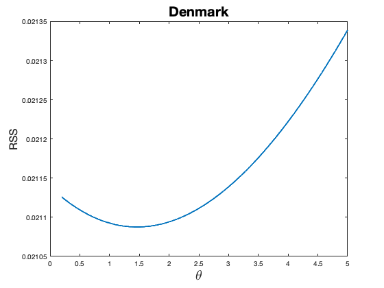
Finally, let us depart from a traditional linear cointegration specification: yt=τ1+τ2​t+ϕ1​xt+uty_{t}=\tau_{1}+\tau_{2}t+\phi_{1}x_{t}+u_{t}. This model cannot incorporate any nonlinear behaviour over time and is therefore ill-suited to fit the data displayed in Figure 4(c). Cointegrating polynomial regressions use integer powers of xtx_{t} to describe the curvature over time. More general, as in Hu et al. 2021, we can allow for an integrated regressor with a flexible power and estimate yt=τ1+τ2​t+ϕ1​xt+ϕ2​xtθ+uty_{t}=\tau_{1}+\tau_{2}t+\phi_{1}x_{t}+\phi_{2}x_{t}^{\theta}+u_{t}. The residual sum of squares (RSS) of the NLS estimator for this specification is shown in Figure 4(d). The absence of a minimum at θ=2\theta=2 casts doubt on the commonly used quadratic specification in xtx_{t}. Additionally, the lack of any minimum might be interpreted as a sign that log per capita GDP is not the source of nonlinearity. This finding is not specific for Belgium. There are no minima in the RSS for 15 out of 18 countries (see Section S8.4). For the remaining three countries – Denmark, France and the Netherlands – minima are found at θ^D​K=1.46\widehat{\theta}_{DK}=1.46, θ^F​R=3.61\widehat{\theta}_{FR}=3.61 and θ^N​L=1.28\widehat{\theta}_{NL}=1.28, respectively. Alternatively, we can describe the nonlinearity in the data using a flexible deterministic trend as in yt=τ1+τ2​t+τ3​tθ+ϕ1​xt+uty_{t}=\tau_{1}+\tau_{2}t+\tau_{3}t^{\theta}+\phi_{1}x_{t}+u_{t}. The RSS in Figure 4(e) now exhibits a clear minimum. Further empirical analysis on individual countries (see Section S8.5 of the Supplement) suggests that: (1) the inclusion of a flexible time trend renders all quadratic effects in squared log per capita GDP insignificant, and (2) models remain well-specified after removing quadratic income effects from the model. These results suggest – albeit in a univariate setting – that flexible time trends gives a more satisfactory (or at least competing) description of the nonlinearities in the data.

5.2 Seemingly Unrelated Regression

The interpretation of a country-specific flexible deterministic trend is complicated because of its high collinearity with GDP per capita. The multivariate analysis of this section allows us to separate country-specific environmental improvements caused by national income growth from global environmental improvements. We study the following six countries (N=6N=6): Austria, Belgium, Finland, the Netherlands, Switzerland, and the UK. The motivation behind this choice is as follows. First, based on data series to ours, Piaggio and Padilla 2012, Mazzanti and Musolesi 2013, and Wagner et al. 2020 report considerable evidence of parameter heterogeneity across countries.1414 14 Parameter heterogeneity is also reported for other data sets. Examples are List and Gallet 1999, Cole 2005, and Dijkgraaf and Vollebergh 2005. The evidence in Mazzanti and Musolesi 2013 is anecdotal in the sense that these authors consider groups of similar countries and find different results for different groups. The lack of overlap among confidence intervals of country-specific parameters has also been interpreted as a sign of heterogeneity (section 4.2 in Piaggio and Padilla 2012). Wagner et al. 2020 explicitly test for various forms of poolability and conclude that pooling is (at most) appropriate for small subgroups of countries. This lack of parameter homogeneity justifies a multivariate approach with small NN rather than a panel setting. Admittedly, in the current time-series setting, studying “large NN” is also infeasible since consistent estimators for (2​N×2​N)(2N\times 2N) long-run covariance matrices are required. Second, prior studies already refute the existence of a carbon dioxide EKC for several countries and little seems lost by excluding these countries from the outset.1515 15 Most of the parameters in the Generalized Cointegrating Polynomial Regression are country-specific. The estimation accuracy of these parameters should deteriorate little when focussing attention on a subset of countries. Losses will occur in the precision of the estimators for τg\tau_{g} and θ\theta. There is thus a trade-off between accurate global trend estimation (improving with large NN) and accurate LRV estimation (deteriorating with large NN). To strike a balance and to connect to the recent literature, we continue the analysis of Wagner et al. 2020 and take N=6N=6. That is, we consider the same countries as in Wagner et al. 2020, who decide on these countries because their prior cointegration analysis “leads to evidence for a quadratic cointegrating EKC including a constant and linear trend”.

Table 3: Parameter estimates and test results for Models (M1)–(M3). The joint pp-value refers to the test with null hypothesis H0:ϕ2,1=…=ϕ2,6=0H_{0}:\phi_{2,1}=\ldots=\phi_{2,6}=0 and is thus inapplicable for Model (M3).
Omitted Global Trend Global Trend
Model (M1) (M2) (M3)
FM-SOLS FM-SUR SimNLS SimNLS SimNLS
ϕ1,i\phi_{1,i} ϕ2,i\phi_{2,i} ϕ1,i\phi_{1,i} ϕ2,i\phi_{2,i} ϕ1,i\phi_{1,i} ϕ2,i\phi_{2,i} ϕ1,i\phi_{1,i} ϕ2,i\phi_{2,i} ϕ1,i\phi_{1,i}
Austria 9.37∗∗∗9.37^{***} −0.43∗∗∗-0.43^{***} 3.96∗3.96^{*} −0.16-0.16 6.42∗∗∗6.42^{***} −0.28-0.28 3.08∗∗∗3.08^{***} −0.09-0.09 1.73∗∗∗1.73^{***}
Belgium 11.78∗∗∗11.78^{***} −0.59∗∗∗-0.59^{***} 9.92∗∗∗9.92^{***} −0.50∗∗∗-0.50^{***} 12.36∗∗∗12.36^{***} −0.62∗⁣∗-0.62^{**} 7.68∗∗∗7.68^{***} −0.36-0.36 1.01∗∗∗1.01^{***}
Finland 16.00∗∗∗16.00^{***} −0.72∗∗∗-0.72^{***} 15.07∗∗∗15.07^{***} −0.68∗∗∗-0.68^{***} 17.18∗∗∗17.18^{***} −0.78∗-0.78^{*} 15.19∗∗∗15.19^{***} −0.65-0.65 2.22∗∗∗2.22^{***}
Netherlands 10.68∗∗∗10.68^{***} −0.51∗∗∗-0.51^{***} 9.58∗∗∗9.58^{***} −0.46∗∗∗-0.46^{***} 9.27∗∗∗9.27^{***} −0.44∗-0.44^{*} 4.97∗∗∗4.97^{***} −0.20-0.20 1.33∗∗∗1.33^{***}
Switzerland 8.17∗∗∗8.17^{***} −0.27∗∗∗-0.27^{***} 7.29∗∗∗7.29^{***} −0.23∗∗∗-0.23^{***} 8.11∗∗∗8.11^{***} −0.28-0.28 0.58∗0.58^{*} 0.100.10 2.55∗∗∗2.55^{***}
UK 9.28∗∗∗9.28^{***} −0.47∗∗∗-0.47^{***} 7.93∗∗∗7.93^{***} −0.40∗∗∗-0.40^{***} 9.16∗∗∗9.16^{***} −0.46∗-0.46^{*} 4.93∗∗∗4.93^{***} −0.21-0.21 1.33∗∗∗1.33^{***}
Joint pp-value 0.00 0.00 0.16 0.39 —
KPSS-statistic 3.45 5.10 3.46 3.48 3.78
τ^​tθ^\widehat{\tau}\,t^{\widehat{\theta}} −0.012​t1.263-0.012\,t^{1.263} −1.374⋅10−5t2.450-1.374\cdot 10^{-5}t^{2.450}
  • •

    Note: Asterisks denote rejection of the null hypothesis at the ∗∗∗1%{}^{***}1\%, 5∗⁣∗%{}^{**}5\%, and ∗10%{}^{*}10\% significance level. Depending on the specific table entry, the null hypothesis refers to coefficient(s) being zero or a well-specified cointegrating relation.

Having decided on the set of countries, we subsequently study the effect of the global flexible trend on EKC evidence. Table 3 shows the estimation results of the quadratic EKC specification

yi,t=τ1,i+τ2,i​t+ϕ1,i​xi,t+ϕ2,i​xi,t2+ui,t.y_{i,t}=\tau_{1,i}+\tau_{2,i}t+\phi_{1,i}x_{i,t}+\phi_{2,i}x_{i,t}^{2}+u_{i,t}. (M1)

This setting (possibly with the additional constraint τ2,i=0\tau_{2,i}=0) has been explored in numerous papers, for example: Selden and Song 1994, Piaggio and Padilla 2012, Chan and Wang 2015, Wagner 2015, Wang et al. 2018, and Wagner et al. 2020. For Model (M1), an inverted-U relationship results when ϕ1,i>0\phi_{1,i}>0 and ϕ2,i<0\phi_{2,i}<0 and empirical evidence hereof is traditionally interpreted as the existence of an EKC. If these coefficients have the correct signs, then the country’s turning point – the level of economic growth at which environmental improvement starts – can be computed as exp(−ϕ1,i/2ϕ2,i)\exp\left(-\phi_{1,i}/2\phi_{2,i}\right). We assess the parameter values and their significance using FM-SOLS and FM-SUR (repeating the analysis of Wagner et al. 2020 for ease of comparison) and the simulated approach of Section 3.2. Regardless of estimation method and country, all coefficient signs are in agreement with the EKC hypothesis. The parameters ϕ1,i\phi_{1,i} are generally significantly different from zero but the significance of ϕ2,i\phi_{2,i} does vary across estimation methods. FM-SOLS and FM-SUR typically (strongly) reject H0:ϕ2,i=0H_{0}:\phi_{2,i}=0 (i=1,…,6i=1,\ldots,6) whereas evidence against these null-hypotheses is less pronounced for the simulation-based approach. The same behaviour emerges when testing ϕ2,1=…=ϕ2,6=0\phi_{2,1}=\ldots=\phi_{2,6}=0 jointly. This pattern reminds of the simulation results in Table 2 where the cross-sectional dimensions N=5N=5 and N=10N=10 cause over-sized tests for FM-SOLS and FM-SUR and conservative tests for simulation-based inference. The KPSS test does not indicate any signs of misspecification. Overall, Model (M1) leads to considerable evidence in favour of a quadratic cointegrating EKC.

The reported evidence in favour of the EKC should not come as surprise. First, the set of countries was selected based on this criteria. Second, the visualisations of the data clearly suggest nonlinear effects (recall Figures 4(a) and 4(c) for the case of Belgium). With Model (M1) being restrictive in the sense that nonlinearities over time are solely incorporable through xi,t2x_{i,t}^{2}, we expect this variable to be important. In line with our proposed Generalized Cointegrating Polynomial Regression (GCPR) framework, we subsequently add a global flexible trend and estimate

yi,t=τg​tθ+τ1,i+τ2,i​t+ϕ1,i​xi,t+ϕ2,i​xi,t2+ui,t.y_{i,t}=\tau_{g}t^{\theta}+\tau_{1,i}+\tau_{2,i}t+\phi_{1,i}x_{i,t}+\phi_{2,i}x_{i,t}^{2}+u_{i,t}. (M2)

From a statistical perspective, the term τg​tθ\tau_{g}t^{\theta} opens a different channel through which nonlinearities can be described. We refer back to the introduction for a further elaboration on this point. From an economic perspective, τg​tθ\tau_{g}t^{\theta} captures changes in CO2 emissions that are common across series and thus unrelated to changes in national GDPs. Parameter inference for Model (M2) is also reported in Table 3. The contributions of xi,t2x_{i,t}^{2} are insignificant for both individual countries and all countries jointly. How about the significance of the global trend? The standard Wald test for τg=0\tau_{g}=0 is invalid because θ\theta is unidentified under the null hypothesis (see Assumption 1 and the related discussion). As a heuristic alternative, we vary θ\theta over the interval [0,2.5][0,2.5] and compute Wald statistics while assuming θ\theta to be fixed. Comparing these Wald statistics to the 95% quantile of a χ2​(1)\chi^{2}(1)-distributed random variable (critical value: 3.842), the range of θ\theta-values from about 0.5 to 1.75 implies a significant global trend (Figure 5). Having estimated θ^=1.263\widehat{\theta}=1.263, our analysis suggests that the global trend and not GDP per capita is the source of nonlinearity. Before interpreting this result, we first verify whether the model with ϕ2,1=…=ϕ2,6=0\phi_{2,1}=\ldots=\phi_{2,6}=0 shows signs of misspecification.

Refer to caption
Figure 5: The magnitude of the Wald test for fixed values of θ\theta when testing H0:τg=0H_{0}:\tau_{g}=0 under Model (M2). Dash lines display the 95% quantile of a chi-squared distributed random variable with 1 degree of freedom (red) and the NLS estimate θ^=1.263\widehat{\theta}=1.263 for specification (M2).

Omitting insignificant parameters from the previous model specification, we arrive at

yi,t=τg​tθ+τ1,i+τ2,i​t+ϕ1,i​xi,t+ui,t.y_{i,t}=\tau_{g}t^{\theta}+\tau_{1,i}+\tau_{2,i}t+\phi_{1,i}x_{i,t}+u_{i,t}. (M3)

Model (M3) is linear in log per capita GDP. The positive parameter estimates for ϕ1,i\phi_{1,i} imply that at a given point in time increases in economic growth imply increases in CO2 emissions. However, as τ^g=−1.374×10⁻⁵\widehat{\tau}_{g}=-1.374\times 10^{-5} and θ^=2.45\widehat{\theta}=2.45, there will be common emission reductions over time. Also, the omission of the quadratic terms in log per capita GDP do not seem to result in a misspecified model. First, the KPSS test does not reject the null of cointegration. Second, there is no (visual) evidence that the linear functional form of (M3) is inappropriate. To arrive at this last conclusion, we compute y~i,t=yi,t−τ^g​tθ^−τ^1,i−τ^2,i​t\widetilde{y}_{i,t}=y_{i,t}-\widehat{\tau}_{g}t^{\widehat{\theta}}-\widehat{\tau}_{1,i}-\widehat{\tau}_{2,i}t and employ the nonparametric kernel estimator from Wang and Phillips 2009 to estimate y~i,t=f⁡(xi,t)+u~i,t\widetilde{y}_{i,t}=f(x_{i,t})+\widetilde{u}_{i,t} for each individual country.1616 16 The properties of nonparametric kernel estimators in nonlinear cointegration models have been studied by Wang and Phillips 2009, Gao et al. 2015 and Wang and Phillips 2016, among others. The latter reference is particularly relevant because it establishes that kernel estimators remain consistent and asymptotically (mixed) normal under serially correlated errors and endogeneity. None of these papers includes deterministic trends in the DGP. However, we conjecture that detrending does not affect the asymptotic properties of the kernel estimator due to the high convergence rates of the trend parameters in comparison to the slow convergence rates of the nonparametric estimator. Our bandwidth choice is h=T−1/3h=T^{-1/3}. Figure 6 shows the nonparametric estimate in blue and the fit of Model (M3) in red. After removal of the global trend, there are some temporary departures from linearity but there is little curvature overall and certainly no visual turning point. In Table 4, we formally test the null of linearity using the model specification test as outlined in section 3 of Wang and Phillips 2016. Based on the full sample, linearity is rejected for Austria only. A comparison with the 95% confidence intervals of the kernel estimate (Figure 6) suggests that this rejection is caused by the sharp decline in CO2 emissions during World War II. We subsequently repeat the analysis using the T=69T=69 observations after 1945. Linearity is never rejected.1717 17 The high pp-values in Table 4 are caused by visually small deviations from the linear trend (see Section S8.6 in the Supplement for detailed graphs). Also, the relatively small sample size (for nonparametric settings) might adversely affect power. Matlab functions for nonparametric kernel regression and specification test are available at https://github.com/HannoReuvers. For remarks on bandwidth choice and detrending, we refer to footnote 16. All this align well with our earlier findings of a relevant global trend and irrelevant quadratic effects in log GDP per capita.

Refer to caption
Figure 6: The 95% (point-wise) confidence intervals of the non-parametric kernel estimate for the relationship between GDP and CO2 emissions (blue) after removal of the country-specific and joint flexible deterministic trends. The red line indicates the linear fit implied by the estimation results of Model (M3). As the sample covers the years 1870–2014 there are several observations during World War I and World War II. The affected ranges of GDP are indicated in grey.
Table 4: Linearity test results. The linearity test is based on the model specification test documented in section 3 of Wang and Phillips 2016. The test is based on the integrated weighted squared deviations between the data and the linear model fit. We report the integration range, the (standardized) test statistic, and the pp-value. Under H0H_{0}, the relationship between (detrended) log CO2 emissions and log GDP per capita is linear.
Full Sample After World War II
range ϕτ0​n​h​Tn\frac{\phi}{\tau_{0}\sqrt{n}h}T_{n} pp-value range ϕτ0​n​h​Tn\frac{\phi}{\tau_{0}\sqrt{n}h}T_{n} pp-value
Austria [8.003,10.635] 8.987 0.000 [8.129,10.635] 0.162 0.871
Belgium [8.389,10.553] 0.299 0.765 [8.923,10.553] 0.076 0.939
Finland [7.494,10.602] 0.105 0.916 [8.693,10.602] 0.020 0.984
Netherlands [8.469,10.728] 0.046 0.964 [8.990,10.728] 0.022 0.982
Switzerland [8.708,10.993] 0.028 0.977 [9.925,10.993] 0.009 0.993
UK [8.641,10.510] 0.022 0.982 [9.242,10.510] 0.021 0.984
  • •

    Note: The asymptotic properties of ϕτ0​n​h​Tn\frac{\phi}{\tau_{0}\sqrt{n}h}T_{n} are established in Wang and Phillips 2016. That is, under suitable conditions, ϕτ0​n​h​Tn→LW​(1,0)\frac{\phi}{\tau_{0}\sqrt{n}h}T_{n}\to L_{W}(1,0) as n→∞n\to\infty with LW​(1,0)L_{W}(1,0) denoting the sojourning time of a standard Brownian motion around zero during the time interval [0,1][0,1]. The pp-values are computed using the cumulative distribution function of LW​(1,0)L_{W}(1,0), see (2.11) in Dong et al. 2017.

The preceding analysis suggests that the global flexible trend captures omitted determinants of CO2 emission levels that have been decreasing over time. In their analysis, Grossman and Krueger 1995 already included a global deterministic trend in their model because they “did not want to attribute to national income growth any improvements in local environmental quality that might actually be due to global advances in the technology for environmental preservation or to an increased global awareness of the severity of environmental problems’’. Indeed, since reliable data on green technology adaptation1818 18 Nordhaus 2014 discusses the link between climate change and technological changes. As another example, Figure 2 in Gillingham and Stock 2018 reports a steady decline in the price of solar panels and a steady growth in solar panel sales. Cheaper solar energy can substitute fossil energy thereby reducing pollution. and global awareness is scarcely available (certainly for time horizons allowing for a cointegration analysis), these variables are likely missing and thus requiring a proxy. Similar remarks are applicable to variables such as pollution control policies1919 19 A policy variable, ‘Repudiation of Contracts by Government’, was included by Panayotou 1997 to proxy the quality of environmental policies and institutions.. In reduced-form models, an EKC finding is typically explained by national income being the proxy for these omitted variables. That is, at higher levels of national income, countries have access to cleaner technologies and its citizens show greater appreciation for the environment and pollution legislation. The current analysis contradicts these income effects and points towards improvements being captured by a global trend.

Our final model specification, Model (M3), is linear in log GDP per capita. Moreover, for a given year, the coefficient estimates suggest that increasing national income by 1% implies an increase in carbon-dioxide emissions of about 1%–2.5% (depending on the country). This result seems plausible for non-carbon-neutral economies. However, CO2 emissions in Austria, Belgium, Finland, the Netherlands, Switzerland, and the UK are jointly reducing at the end of the sample. What cause these global emission reductions? Mazzanti and Musolesi 2013 suggest that conglomerates of countries anticipate and respond to international climate agreements such as the Rio convention (1992) and Kyoto protocol (adopted in 1997; operational since 2005). Interestingly, the latter agreement contains emission reduction targets to be reached in 2020 and such ‘‘working-towards-a-common-reduction-deadline’’ does point towards a time effect.2020 20 According to the Doha amendment of the Kyoto protocol, the reduction commitments were 92% (over the period 2008–2012) and 80% (over the period 2013–2020) of 1990 emission levels for Austria, Belgium, Finland, the Netherlands and the UK. For Switzerland, the reduction target was also 92% (over the period 2008–2012) but 84.2% (over the period 2013–2020). (source: https://unfccc.int/files/kyoto_protocol/application/pdf/kp_doha_amendment_english.pdf). Alternatively, given our sample of European countries, EU coordinated emission reduction efforts like the EU Emissions Trading System (ETS) can be a driving force behind these common emission decreases.

6 Summary and Conclusion

In this paper we have extended the Seemingly Unrelated Cointegrating Polynomial Regression (SUCPR) model of Wagner et al. 2020 with a global power law deterministic trend. This multivariate specification allows us to disentangle national income and unobserved time effects. The importance of this separation is well-documented (see, e.g. Vollebergh et al. 2009 and Mazzanti and Musolesi 2013) but a methodological approach accounting for nonstationary regressors is currently unavailable. We fill this gap.

The unknown powers of the global trend are estimated jointly with the parameters in the cointegrating relation. The limiting distribution is nonstandard due to a non-diagonal scaling matrix and second order bias terms. We therefore suggest a simulation-based approach to conduct inference. The usual subsampling KPSS-type for stationarity of the innovations of the nonlinear cointegrating relation remains valid. Our results are supported by Monte Carlo simulation. The empirical application on the Environmental Kuznets Curve shows that a flexible trend can fully capture the nonlinearity in the data thereby making higher order powers of log per capita GDP redundant. Our resulting model is linear in log per capita GDP and suggests an alternative explanation in which time effects – e.g. technological progress, increasing environmental awareness, tightening pollution policy – rather than economic growth cause the recent slowdown in CO2 emissions. Contrary to the opening quote in the introduction, our analysis suggests that CO2 emissions increase with economic growth. Carbon dioxide emissions do decrease due to time effects.

7 Acknowledgements

Earlier versions of this paper have been presented at the 2019 CFE meeting in London, the Econometrics Internal Seminar (EIS) at Erasmus University Rotterdam, and the Brownbag Seminar at Vrije Universiteit Amsterdam. We gratefully acknowledge the comments by the participants. We extend our thanks to Eric Beutner, Dick van Dijk, Stephan Smeekes, and Xiaohu Wang for their valuable feedback. All remaining errors are our own.

References

  • Adams and Essex (2016) Adams, R. A. and C. Essex (2016). Calculus: A Complete Course. Pearson Canada.
  • Al-Mulali and Ozturk (2016) Al-Mulali, U. and I. Ozturk (2016). The investigation of Environmental Kuznets Curve hypothesis in the advanced economies: The role of energy prices. Renewable and Sustainable Energy Reviews 54, 1622–1631.
  • Andrews and Cheng (2012) Andrews, D. W. and X. Cheng (2012). Estimation and inference with weak, semi-strong, and strong identification. Econometrica 80, 2153–2211.
  • Andrews (1991) Andrews, D. W. K. (1991). Heteroskedasticity and autocorrelation consistent covariance matrix estimation. Econometrica 59, 817–858.
  • Andrews and Sun (2004) Andrews, D. W. K. and Y. Sun (2004). Adaptive local polynomial whittle estimation of long-range dependence. Econometrica 72, 569–614.
  • Baek et al. (2015) Baek, Y. I., S. J. Cho, and P. C. B. Phillips (2015). Testing linearity using power transforms of regressors. Journal of Econometrics 187, 376–384.
  • Bergamelli et al. (2019) Bergamelli, M., A. Bianchi, L. Khalaf, and G. Urga (2019). Combining p-values to test for multiple structural breaks in cointegrated regressions. Journal of Econometrics 211, 461–482.
  • Beutner et al. (2020) Beutner, E., Y. Lin, and S. Smeekes (2020). GLS estimation and confidence sets for the date of a single break in models with trends. Working Paper.
  • Carson (2009) Carson, R. T. (2009). The Environmental Kuznets Curve: seeking empirical regularity and theoretical structure. Review of Environmental Economics and Policy 4, 3–23.
  • Chan and Wang (2015) Chan, N. and Q. Wang (2015). Nonlinear regressions with nonstationary time series. Journal of Econometrics 185, 182–195.
  • Chang et al. (2001) Chang, Y., J. Y. Park, and P. C. B. Phillips (2001). Nonlinear econometric models with cointegrated and deterministically trending regressors. The Econometrics Journal 4, 1–36.
  • Cho and Phillips (2018) Cho, J. S. and P. C. B. Phillips (2018). Sequentially testing polynomial model hypotheses using power transforms of regressors. Journal of Applied Econometrics 33, 141–159.
  • Choi and Saikkonen (2010) Choi, I. and P. Saikkonen (2010). Tests for nonlinear cointegration. Econometric Theory 26, 682–709.
  • Cole (2005) Cole, M. (2005). Re-examining the pollution-income relationship: A random coefficients approach. Economics Bulletin 14, 1–7.
  • Dasgupta et al. (2002) Dasgupta, S., B. K. H. Wang, and D. Wheeler (2002). Confronting the Environmental Kuznets Curve. Journal of Economic Perspectives 16, 147–168.
  • Davies (1977) Davies, R. B. (1977). Hypothesis testing when a nuisance parameter is present only under the alternative. Biometrika 64, 247–254.
  • Davies (1987) Davies, R. B. (1987). Hypothesis testing when a nuisance parameter is present only under the alternative. Biometrika 74, 33–43.
  • Dijkgraaf and Vollebergh (2005) Dijkgraaf, E. and H. R. J. Vollebergh (2005). A test for parameter homogeneity in CO2 panel EKC estimations. Environmental and Resource Economics 32, 229–239.
  • Dong et al. (2017) Dong, C., J. Gao, D. Tjøstheim, and J. Yin (2017). Specification testing for nonlinear multivariate cointegrating regressions. Journal of Econometrics 200, 104–117.
  • Dufour (2006) Dufour, J.-M. (2006). Monte Carlo tests with nuisance parameters: A general approach to finite-sample inference and nonstandard asymptotics. Journal of Econometrics 133, 443–477.
  • Dufour and Khalaf (2002) Dufour, J.-M. and L. Khalaf (2002). Simulation based finite and large sample tests in multivariate regressions. Journal of Econometrics 111, 303–322.
  • Duggal et al. (1999) Duggal, V. G., C. Saltzman, and L. R. Klein (1999). Infrastructure and productivity: a nonlinear approach. Journal of Econometrics 92, 47–74.
  • Duggal et al. (2007) Duggal, V. G., C. Saltzman, and L. R. Klein (2007). Infrastructure and productivity: An extension to private infrastructure and it productivity. Journal of Econometrics 140, 485–502.
  • Galeotti et al. (2009) Galeotti, M., M. Manera, and A. Lanza (2009). On the robustness of robustness checks of the environmental Kuznets curve hypothesis. Environmental and Resource Economics 42, 551.
  • Gao et al. (2015) Gao, J., S. Kanaya, D. Li, and D. Tjøstheim (2015). Uniform consistency for nonparametric estimators in null recurrent time series. Econometric Theory 31, 911–952.
  • Gao et al. (2020) Gao, J., O. Linton, and B. Peng (2020). Inference on a semiparametric model with global power law and local nonparametric trends. Econometric Theory 36, 223–249.
  • Gillingham and Stock (2018) Gillingham, K. and J. H. Stock (2018). The cost of reducing greenhouse gas emissions. Journal of Economic Perspectives 32, 53–72.
  • Gillingham and Nordhaus (2018) Gillingham, P. C. K. and W. Nordhaus (2018). Uncertainty in forecasts of long-run economic growth. Proceedings of the National Academy of Sciences 115, 5409–5414.
  • Grossman and Krueger (1995) Grossman, G. M. and A. B. Krueger (1995). Economic growth and the environment. The Quarterly Journal of Economics 110, 353–377.
  • Hamilton (1994) Hamilton, J. D. (1994). Time Series Analysis. Princeton University Press.
  • Harbaugh et al. (2002) Harbaugh, W. T., A. Levinson, and D. M. Wilson (2002). Reexamining the empirical evidence for an environmental Kuznets curve. Review of Economics and Statistics 84, 541–551.
  • Hong and Phillips (2010) Hong, S. H. and P. C. B. Phillips (2010). Testing linearity in cointegrating relations with an application to purchasing power parity. Journal of Business & Economic Statistics 28, 96–114.
  • Hu et al. (2021) Hu, Z., P. C. B. Phillips, and Q. Wang (2021). Nonlinear cointegrating power function regression with endogeneity. Econometric Theory 37, 1173–1213.
  • Jalil and Feridun (2011) Jalil, A. and M. Feridun (2011). The impact of growth, energy and financial development on the environment in China: A cointegration analysis. Energy Economics 33, 284–291.
  • Jansson (2002) Jansson, M. (2002). Consistent covariance matrix estimation for linear processes. Econometric Theory 18, 1449–1459.
  • Jiang et al. (2019) Jiang, B., Y. Lu, and J. Y. Park (2019). Testing for stationary at high frequency. Journal of Econometrics 215, 341–374.
  • Klein et al. (2004) Klein, L. R., V. G. Duggal, and C. Saltzman (2004). Contributions of input-output analysis to the understanding of technological change: the information sector in the United States. In E. Dietzenbacher and M. L. Lahr (Eds.), Wassily Leontief and Input-output Economics, Chapter 17, pp. 311–336. Cambridge University Press.
  • Kwiatkowski et al. (1992) Kwiatkowski, D., P. C. B. Phillips, P. Schmidt, and Y. Shin (1992). Testing the null hypothesis of stationarity against the alternative of a unit root: How sure are we that economic time series have a unit root? Journal of Econometrics 54, 159–178.
  • Li and Linton (2020) Li, S. and O. Linton (2020). When will the covid-19 pandemic peak? Journal of Econometrics 220, 130–157.
  • Lin and Reuvers (2020) Lin, Y. and H. Reuvers (2020). Efficient estimation by fully modified GLS with an application to the Environmental Kuznets Curve. Working paper.
  • Lin et al. (2020) Lin, Y., Y. Tu, and Q. Yao (2020). Estimation for double-nonlinear cointegration. Journal of Econometrics 216, 175–191.
  • Linton and Wang (2016) Linton, O. and Q. Wang (2016). Nonparametric transformation regression with nonstationary data. Econometric Theory 32, 1–29.
  • List and Gallet (1999) List, J. A. and C. A. Gallet (1999). The environmental Kuznets curve: Does one size fit all? Ecological Economics 31, 409–423.
  • Maranzano et al. (2021) Maranzano, P., J. P. C. Bento, and M. Manera (2021). The role of education and income inequality on environmental quality. A panel data analysis of the EKC hypothesis on OECD. Nota di Lavoro 8.2021, Milano, Italy: Fondazione Eni Enrico Mattei.
  • Mazzanti and Musolesi (2013) Mazzanti, M. and A. Musolesi (2013). The heterogeneity of carbon kuznets curves for advanced countries: Comparing homogeneous, heterogeneous and shrinkage/bayesian estimators. Applied Economics 45, 3827–3842.
  • Nordhaus (2013) Nordhaus, W. D. (2013). The Climate Casino: Risk, Uncertainty, and Economics for a Warming World. Yale University Press.
  • Nordhaus (2014) Nordhaus, W. D. (2014). The perils of the learning model for modeling endogenous technological change. The Energy Journal 35, 1–13.
  • Panayotou (1997) Panayotou, T. (1997). Demystifying the environmental kuznets curve: Turning a black box into a policy tool. Environment and Development Economics 2, 465–484.
  • Park (2002) Park, J. Y. (2002). An invariance principle for sieve bootstrap in time series. Econometric Theory 18, 469–490.
  • Park and Phillips (1999) Park, J. Y. and P. C. B. Phillips (1999). Asymptotics for nonlinear transformations of integrated time series. Econometric Theory 15, 269–298.
  • Park and Phillips (2001) Park, J. Y. and P. C. B. Phillips (2001). Nonlinear regressions with integrated time series. Econometrica 69, 117–161.
  • Perron and Yabu (2009) Perron, P. and T. Yabu (2009). Estimating deterministic trends with an integrated or stationary noise component. Journal of Econometrics 151, 56–69.
  • Perron and Zhu (2005) Perron, P. and X. Zhu (2005). Structural breaks with deterministic and stochastic trends. Journal of Econometrics 129, 65–119.
  • Phillips (1995) Phillips, P. C. B. (1995). Fully modified least squares and vector autoregression. Econometrica 63, 1023–1078.
  • Phillips (2007) Phillips, P. C. B. (2007). Regression with slowly varying regressors and nonlinear trends. Econometric Theory 23, 557–614.
  • Phillips and Hansen (1990) Phillips, P. C. B. and B. E. Hansen (1990). Statistical inference in instrumental variables regression with I(1) processes. The Review of Economic Studies 57, 99–125.
  • Piaggio and Padilla (2012) Piaggio, M. and E. Padilla (2012). CO2 emissions and economic activity: Heterogeneity across countries and non-stationary series. Energy Policy 46, 370–381.
  • Robinson (2012) Robinson, P. M. (2012). Inference on power law spatial trends. Bernoulli 18, 644–677.
  • Romano and Wolf (2001) Romano, J. P. and M. Wolf (2001). Subsampling intervals in autoregressive models with linear time trend. Econometrica 69, 1283–1314.
  • Saikkonen (1992) Saikkonen, P. (1992). Estimation and testing of cointegrated systems by an autoregressive approximation. Econometric Theory 8, 1–27.
  • Selden and Song (1994) Selden, T. M. and D. Song (1994). Environmental quality and development: Is there a Kuznets curve for air pollution emissions? Journal of Environmental Economics and Management 27, 147–162.
  • Soong (1973) Soong, T. T. (1973). Random Differential Equations in Science and Engineering. Academic Press, Inc.
  • Stern (2004) Stern, D. I. (2004). The rise and fall of the environmental kuznets curve. World Development 32, 1419–1439.
  • Stern (2017) Stern, D. I. (2017). The environmental Kuznets curve after 25 years. Journal of Bioeconomics 19, 7–28.
  • Stypka et al. (2017) Stypka, O., M. Wagner, P. Grabarczyk, and R. Kawka (2017). The asymptotic validity of “standard” fully modified OLS estimation and inference in cointegrating polynomial regressions. Working Paper.
  • Tanaka (2017) Tanaka, K. (2017). Time Series Analysis: Nonstationary and Noninvertible Distribution Theory. John Wiley & Sons.
  • Vogelsang and Wagner (2014) Vogelsang, T. J. and M. Wagner (2014). Integrated modified OLS estimation and fixed-b inference for cointegrating regressions. Journal of Econometrics 178, 741–760.
  • Vollebergh et al. (2009) Vollebergh, H. R. J., B. Melenberg, and E. Dijkgraaf (2009). Identifying reduced-form relations with panel data: The case of pollution and income. Journal of Environmental Economics and Management 58, 27–42.
  • Wagner (2015) Wagner, M. (2015). The Environmental Kuznets Curve, cointegration and nonlinearity. Journal of Applied Econometrics 30, 948–967.
  • Wagner et al. (2020) Wagner, M., P. Grabarczyk, and S. H. Hong (2020). Fully modified OLS estimation and inference for seemingly unrelated cointegrating polynomial regressions and the Environmental Kuznets Curve for carbon dioxide emissions. Journal of Econometrics 214, 216–255.
  • Wagner and Hong (2016) Wagner, M. and S. H. Hong (2016). Cointegrating polynomial regressions: Fully modified OLS estimation and inference. Econometric Theory 32, 1289–1315.
  • Wang and Phillips (2009) Wang, Q. and P. C. B. Phillips (2009). Structural nonparametric cointegrating regression. Econometrica 77, 1901–1948.
  • Wang and Phillips (2012) Wang, Q. and P. C. B. Phillips (2012). A specification test for nonlinear nonstationary models. The Annals of Statistics 40, 727–758.
  • Wang and Phillips (2016) Wang, Q. and P. C. B. Phillips (2016). Nonparametric cointegrating regression with endogeneity and long memory. Econometric Theory 32, 359–401.
  • Wang et al. (2018) Wang, Q., D. Wu, and K. Zhu (2018). Model checks for nonlinear cointegrating regression. Journal of Econometrics 207, 261–284.

Appendix A Proofs for Main Theorems

Proof of Theorem 1 In view of the identity ‖𝒂+𝒃‖2=‖𝒂‖2+‖𝒃‖2+2​𝒂′​𝒃\left\lVert\bm{a}+\bm{b}\right\rVert^{2}=\left\lVert\bm{a}\right\rVert^{2}+\left\lVert\bm{b}\right\rVert^{2}+2\bm{a}^{\prime}\bm{b}, we also have

QT​(𝜸)=12​∑t=1T‖𝒚t−𝒁t′​𝜷‖2−τg​∑t=1Ttθ​(𝒚t−𝒁t′​𝜷)′​ıN+12​N​τg2​∑t=1Tt2​θ.Q_{T}(\bm{\gamma})=\frac{1}{2}\sum_{t=1}^{T}\left\|\bm{y}_{t}-\bm{Z}_{t}^{\prime}\bm{\beta}\right\|^{2}-\tau_{g}\sum_{t=1}^{T}t^{\theta}\left(\bm{y}_{t}-\bm{Z}_{t}^{\prime}\bm{\beta}\right)^{\prime}\bm{\imath}_{N}+\frac{1}{2}N\tau_{g}^{2}\sum_{t=1}^{T}t^{2\theta}.

The proof proceeds along the lines of Lemma 1 of Andrews and Sun 2004 and Theorem 3.1 of Chan and Wang 2015. The proofs separate into two parts. The first part uses a Taylor expansion of QT​(𝜸)Q_{T}(\bm{\gamma}) around QT​(𝜸0)Q_{T}(\bm{\gamma}_{0}) to recover a quadratic approximation for QT​(𝜸)Q_{T}(\bm{\gamma}) on the set 𝚪δ,kT⊆𝚪\bm{\varGamma}_{\delta,k_{T}}\subseteq\bm{\varGamma}. In the second part, we obtain the limiting distribution from this quadratic approximation.

Part 1: Let {kT,T≥1}\{k_{T},T\geq 1\} denote a deterministic sequence such that kT→∞k_{T}\to\infty as T→∞T\to\infty. Define 𝚪δ,kT={𝜸∈𝚪:‖𝑮𝜸0,T(𝜸−𝜸0)‖≤kT,‖𝜸−𝜸0‖≤δ}\bm{\varGamma}_{\delta,k_{T}}=\left\{\bm{\gamma}\in\bm{\varGamma}:\penalty\ \left\|\bm{G}_{\bm{\gamma}_{0},T}\left(\bm{\gamma}-\bm{\gamma}_{0}\right)\right\|\leq k_{T},\penalty\ \left\|\bm{\gamma}-\bm{\gamma}_{0}\right\|\leq\delta\right\} and select a δ>0\delta>0 such that QT​(⋅)Q_{T}(\cdot) is twice differentiable on {𝜸∈ℝp+2:‖𝜸−𝜸0‖≤δ}⊂𝚪\{\bm{\gamma}\in\mathbb{R}^{p+2}:\,\left\|\bm{\gamma}-\bm{\gamma}_{0}\right\|\leq\delta\}\subset\bm{\varGamma}. For any 𝜸∈𝚪δ,kT\bm{\gamma}\in\bm{\varGamma}_{\delta,k_{T}}, the Taylor expansion of QT​(𝜸)Q_{T}(\bm{\gamma}) around 𝜸0\bm{\gamma}_{0} reads

QT​(𝜸)\displaystyle Q_{T}(\bm{\gamma}) −QT​(𝜸0)=Q˙T′​(𝜸0)​(𝜸−𝜸0)+12​(𝜸−𝜸0)′​Q¨T​(𝜸¯)​(𝜸−𝜸0)\displaystyle-Q_{T}(\bm{\gamma}_{0})=\dot{Q}_{T}^{\prime}(\bm{\gamma}_{0})(\bm{\gamma}-\bm{\gamma}_{0})+\frac{1}{2}(\bm{\gamma}-\bm{\gamma}_{0})^{\prime}\ddot{Q}_{T}(\bar{\bm{\gamma}})(\bm{\gamma}-\bm{\gamma}_{0}) (A.1)
=Q˙T′​(𝜸0)​(𝜸−𝜸0)+12​(𝜸−𝜸0)′​[Q¨T​(𝜸¯)−Q¨T​(𝜸0)−Q¨T,2​(𝜸0)+Q¨T,1​(𝜸0)]​(𝜸−𝜸0),\displaystyle=\dot{Q}_{T}^{\prime}(\bm{\gamma}_{0})(\bm{\gamma}-\bm{\gamma}_{0})+\frac{1}{2}(\bm{\gamma}-\bm{\gamma}_{0})^{\prime}\left[\ddot{Q}_{T}(\bar{\bm{\gamma}})-\ddot{Q}_{T}(\bm{\gamma}_{0})-\ddot{Q}_{T,2}(\bm{\gamma}_{0})+\ddot{Q}_{T,1}(\bm{\gamma}_{0})\right](\bm{\gamma}-\bm{\gamma}_{0}),

where 𝜸¯\bar{\bm{\gamma}} is a point on the line segment connecting 𝜸\bm{\gamma} and 𝜸0\bm{\gamma}_{0}, and the various derivatives of QTQ_{T} are

Q˙T​(𝜸0)\displaystyle\dot{Q}_{T}(\bm{\gamma}_{0}) =−∑t=1T[ıN′​τg​0​tθ0​ln⁡tıN′​tθ0𝒁t]𝒖t,\displaystyle=-\sum_{t=1}^{T}\left[\begin{smallmatrix}\bm{\imath}_{N}^{\prime}\tau_{g0}\,t^{\theta_{0}}{\ln t}\\ \bm{\imath}_{N}^{\prime}\,t^{\theta_{0}}\\ \bm{Z}_{t}\end{smallmatrix}\right]\bm{u}_{t},
Q¨T​(𝜸)\displaystyle\ddot{Q}_{T}(\bm{\gamma}) =∑t=1T[−τg​tθ​(ln⁡t)2​(𝒚t−𝒁t′​𝜷)′​ıN+2​N​τg2​t2​θ​(ln⁡t)2−tθ​ln⁡t​(𝒚t−𝒁t′​𝜷)′​ıN+2​N​τg​t2​θ​ln⁡tτg​tθ​ln⁡t​ıN′​𝒁t′−tθ​ln⁡t​(𝒚t−𝒁t′​𝜷)′​ıN+2​N​τg​t2​θ​ln⁡tN​t2​θtθ​ıN′​𝒁t′τg​tθ​ln⁡t​𝒁t​ıNtθ​𝒁t​ıN𝒁t​𝒁t′],\displaystyle=\sum_{t=1}^{T}\left[\begin{smallmatrix}-\tau_{g}t^{\theta}(\ln{t})^{2}\left(\bm{y}_{t}-\bm{Z}_{t}^{\prime}\bm{\beta}\right)^{\prime}\bm{\imath}_{N}+2N\tau_{g}^{2}t^{2\theta}(\ln{t})^{2}\;&-t^{\theta}\ln{t}\left(\bm{y}_{t}-\bm{Z}_{t}^{\prime}\bm{\beta}\right)^{\prime}\bm{\imath}_{N}+2N\tau_{g}t^{2\theta}\ln{t}\;&\tau_{g}t^{\theta}\ln{t}\,\bm{\imath}_{N}^{\prime}\bm{Z}_{t}^{\prime}\\ -t^{\theta}\ln{t}\left(\bm{y}_{t}-\bm{Z}_{t}^{\prime}\bm{\beta}\right)^{\prime}\bm{\imath}_{N}+2N\tau_{g}t^{2\theta}\ln{t}&Nt^{2\theta}&t^{\theta}\bm{\imath}_{N}^{\prime}\bm{Z}_{t}^{\prime}\\ \tau_{g}t^{\theta}\ln{t}\,\bm{Z}_{t}\bm{\imath}_{N}&t^{\theta}\bm{Z}_{t}\bm{\imath}_{N}&\bm{Z}_{t}\bm{Z}_{t}^{\prime}\end{smallmatrix}\right],
Q¨T​(𝜸0)\displaystyle\ddot{Q}_{T}(\bm{\gamma}_{0}) =∑t=1T[N​τg​02​t2​θ0​(ln⁡t)2−τg​0​tθ0​(ln⁡t)2​𝒖t′​ıNN​τg​0​t2​θ0​ln⁡t−tθ0​ln⁡t​𝒖t′​ıNτg​0​tθ0​ln⁡t​ıN′​𝒁t′N​τg​0​t2​θ0​ln⁡t−tθ0​ln⁡t​𝒖t′​ıNN​t2​θ0tθ0​ıN′​𝒁t′τg​0​tθ0​ln⁡t​𝒁t​ıNtθ0​𝒁t​ıN𝒁t​𝒁t′]\displaystyle=\sum_{t=1}^{T}\left[\begin{smallmatrix}N\tau_{g0}^{2}t^{2\theta_{0}}(\ln{t})^{2}-\tau_{g0}t^{\theta_{0}}(\ln{t})^{2}\bm{u}_{t}^{\prime}\bm{\imath}_{N}\;&N\tau_{g0}t^{2\theta_{0}}\ln{t}-t^{\theta_{0}}\ln{t}\,\bm{u}_{t}^{\prime}\bm{\imath}_{N}\;&\tau_{g0}t^{\theta_{0}}\ln{t}\bm{\imath}_{N}^{\prime}\bm{Z}_{t}^{\prime}\\ N\tau_{g0}t^{2\theta_{0}}\ln{t}-t^{\theta_{0}}\ln{t}\,\bm{u}_{t}^{\prime}\bm{\imath}_{N}&Nt^{2\theta_{0}}&t^{\theta_{0}}\bm{\imath}_{N}^{\prime}\bm{Z}_{t}^{\prime}\\ \tau_{g0}t^{\theta_{0}}\ln{t}\,\bm{Z}_{t}\bm{\imath}_{N}&t^{\theta_{0}}\bm{Z}_{t}\bm{\imath}_{N}&\bm{Z}_{t}\bm{Z}_{t}^{\prime}\end{smallmatrix}\right]
=∑t=1T[N​τg​02​t2​θ0​(ln⁡t)2N​τg​0​t2​θ0​ln⁡tτg​0​tθ0​ln⁡t​ıN′​𝒁t′N​τg​0​t2​θ0​ln⁡tN​t2​θ0tθ0​ıN′​𝒁t′τg​0​tθ0​ln⁡t​𝒁t​ıNtθ0​𝒁t​ıN𝒁t​𝒁t′]−∑t=1Ttθ0​ln⁡t​[τg​0​ln⁡t110𝐎]​𝒖t′​ıN\displaystyle=\sum_{t=1}^{T}\begin{bmatrix}N\tau_{g0}^{2}t^{2\theta_{0}}(\ln{t})^{2}&N\tau_{g0}t^{2\theta_{0}}\ln{t}&\tau_{g0}t^{\theta_{0}}\ln{t}\,\bm{\imath}_{N}^{\prime}\bm{Z}_{t}^{\prime}\\ N\tau_{g0}t^{2\theta_{0}}\ln{t}&Nt^{2\theta_{0}}&t^{\theta_{0}}\bm{\imath}_{N}^{\prime}\bm{Z}_{t}^{\prime}\\ \tau_{g0}t^{\theta_{0}}\ln{t}\,\bm{Z}_{t}\bm{\imath}_{N}&t^{\theta_{0}}\bm{Z}_{t}\bm{\imath}_{N}&\bm{Z}_{t}\bm{Z}_{t}^{\prime}\end{bmatrix}-\sum_{t=1}^{T}t^{\theta_{0}}\ln{t}\begin{bmatrix}\tau_{g0}\ln{t}&1&\\ 1&0&\\ &&\mathbf{O}\end{bmatrix}\bm{u}_{t}^{\prime}\bm{\imath}_{N}
=:Q¨T,1​(𝜸0)−Q¨T,2​(𝜸0).\displaystyle=:\ddot{Q}_{T,1}(\bm{\gamma}_{0})-\ddot{Q}_{T,2}(\bm{\gamma}_{0}).

Defining RT​(𝜸¯,𝜸0)=12​(𝜸−𝜸0)′​[Q¨T​(𝜸¯)−Q¨T​(𝜸0)−Q¨T,2​(𝜸0)]​(𝜸−𝜸0)R_{T}(\bar{\bm{\gamma}},\bm{\gamma}_{0})=\frac{1}{2}(\bm{\gamma}-\bm{\gamma}_{0})^{\prime}\left[\ddot{Q}_{T}(\bar{\bm{\gamma}})-\ddot{Q}_{T}(\bm{\gamma}_{0})-\ddot{Q}_{T,2}(\bm{\gamma}_{0})\right](\bm{\gamma}-\bm{\gamma}_{0}), 𝑨T:=𝑮𝜸0,T′−1​Q¨T,1​(𝜸0)​𝑮𝜸0,T−1\bm{A}_{T}:=\bm{G}_{\bm{\gamma}_{0},T}^{\prime-1}\ddot{Q}_{T,1}(\bm{\gamma}_{0})\bm{G}_{\bm{\gamma}_{0},T}^{-1}, and 𝒃T:=−𝑮𝜸0,T′−1​Q˙T​(𝜸0)\bm{b}_{T}:=-\bm{G}_{\bm{\gamma}_{0},T}^{\prime-1}\dot{Q}_{T}(\bm{\gamma}_{0}), we finally arrive at

QT\displaystyle Q_{T} (𝜸)−QT​(𝜸0)=−𝒃T′​[𝑮𝜸0,T​(𝜸−𝜸0)]+12​[𝑮𝜸0,T​(𝜸−𝜸0)]′​𝑨T​[𝑮𝜸0,T​(𝜸−𝜸0)]+RT​(𝜸¯,𝜸0)\displaystyle(\bm{\gamma})-Q_{T}(\bm{\gamma}_{0})=-\bm{b}_{T}^{\prime}\big[\bm{G}_{\bm{\gamma}_{0},T}(\bm{\gamma}-\bm{\gamma}_{0})\big]+\frac{1}{2}\big[\bm{G}_{\bm{\gamma}_{0},T}(\bm{\gamma}-\bm{\gamma}_{0})\big]^{\prime}\bm{A}_{T}\big[\bm{G}_{\bm{\gamma}_{0},T}(\bm{\gamma}-\bm{\gamma}_{0})\big]+R_{T}(\bar{\bm{\gamma}},\bm{\gamma}_{0}) (A.2)
=12​[𝑮𝜸0,T​(𝜸−𝜸0)−𝑨T−1​𝒃T]′​𝑨T​[𝑮𝜸0,T​(𝜸−𝜸0)−𝑨T−1​𝒃T]−12​𝒃T′​𝑨T−1​𝒃T+RT​(𝜸¯,𝜸0).\displaystyle=\frac{1}{2}\left[\bm{G}_{\bm{\gamma}_{0},T}(\bm{\gamma}-\bm{\gamma}_{0})-\bm{A}_{T}^{-1}\bm{b}_{T}\right]^{\prime}\bm{A}_{T}\left[\bm{G}_{\bm{\gamma}_{0},T}(\bm{\gamma}-\bm{\gamma}_{0})-\bm{A}_{T}^{-1}\bm{b}_{T}\right]-\frac{1}{2}\bm{b}_{T}^{\prime}\bm{A}_{T}^{-1}\bm{b}_{T}+R_{T}(\bar{\bm{\gamma}},\bm{\gamma}_{0}).

Part 2: For any ε>0\varepsilon>0, let 𝚪T​(ε)={𝜸∈𝚪:‖𝑮𝜸0,T​(𝜸−𝜸0)−𝑨T−1​𝒃T‖≤ε}\bm{\varGamma}_{T}(\varepsilon)=\big\{\bm{\gamma}\in\bm{\varGamma}:\penalty\ \big\|\bm{G}_{\bm{\gamma}_{0},T}(\bm{\gamma}-\bm{\gamma}_{0})-\bm{A}_{T}^{-1}\bm{b}_{T}\big\|\leq\varepsilon\big\}. We shall show that the minimum of QT​(⋅)Q_{T}(\cdot) over 𝜸∈𝚪T​(ε)\bm{\gamma}\in\bm{\varGamma}_{T}(\varepsilon) is attained in the interior of 𝚪T​(ε)\bm{\varGamma}_{T}(\varepsilon). The next two statements are proven later:

  1. (a)

    sup𝜸∈𝚪δ,kT‖𝑮𝜸0,T′−1​[Q¨T​(𝜸)−Q¨T​(𝜸0)]​𝑮𝜸0,T−1‖=op​(1)\sup_{\bm{\gamma}\in\bm{\varGamma}_{\delta,k_{T}}}\left\|\bm{G}_{\bm{\gamma}_{0},T}^{\prime-1}\big[\ddot{Q}_{T}(\bm{\gamma})-\ddot{Q}_{T}(\bm{\gamma}_{0})\big]\bm{G}_{\bm{\gamma}_{0},T}^{-1}\right\|=o_{p}(1);

  2. (b)

    𝑨T−1​𝒃T=Op​(1)\bm{A}_{T}^{-1}\bm{b}_{T}=O_{p}(1), where 𝑨T​⟶dT→∞​𝑨∞\bm{A}_{T}\overset{T\rightarrow\infty}{\longrightarrow_{d}}\bm{A}_{\infty} with ℙ⁡(𝑨∞>0)=1\mathbb{P}\left(\bm{A}_{\infty}>0\right)=1.

Given claim (b), for any ε>0\varepsilon>0, we have ℙ⁡(𝚪T​(ε)⊂𝚪δ,kT)→1\mathbb{P}\left(\bm{\varGamma}_{T}(\varepsilon)\subset\bm{\varGamma}_{\delta,k_{T}}\right)\rightarrow 1 as T→∞T\rightarrow\infty because ‖𝑮𝜸0,T−1‖→0\|\bm{G}_{\bm{\gamma}_{0},T}^{-1}\|\to 0. Define 𝜸T∗=𝜸0+𝑮𝜸0,T−1​𝑨T−1​𝒃T\bm{\gamma}_{T}^{*}=\bm{\gamma}_{0}+\bm{G}_{\bm{\gamma}_{0},T}^{-1}\bm{A}_{T}^{-1}\bm{b}_{T}. Clearly, 𝜸T∗\bm{\gamma}_{T}^{*} is an interior point of 𝚪T​(ε)\bm{\varGamma}_{T}(\varepsilon) as long as ε>0\varepsilon>0. Subsequently select a 𝜸ε∈∂𝚪T​(ε)\bm{\gamma}_{\varepsilon}\in\partial\bm{\varGamma}_{T}(\varepsilon), i.e. 𝜸ε\bm{\gamma}_{\varepsilon} is a boundary point of 𝚪T​(ε)\bm{\varGamma}_{T}(\varepsilon). From (A.2), we have

QT​(𝜸ε)−QT​(𝜸T∗)\displaystyle Q_{T}(\bm{\gamma}_{\varepsilon})-Q_{T}(\bm{\gamma}_{T}^{*}) =[QT​(𝜸ε)−QT​(𝜸0)]−[QT​(𝜸T∗)−QT​(𝜸0)]\displaystyle=\left[Q_{T}(\bm{\gamma}_{\varepsilon})-Q_{T}(\bm{\gamma}_{0})\right]-\left[Q_{T}(\bm{\gamma}_{T}^{*})-Q_{T}(\bm{\gamma}_{0})\right]
=[12​𝝁T′​𝑨T​𝝁T−12​𝒃T′​𝑨T−1​𝒃T+RT​(𝜸¯ε,𝜸0)]−[−12​𝒃T′​𝑨T−1​𝒃T+RT​(𝜸¯T∗,𝜸0)]\displaystyle=\left[\frac{1}{2}\bm{\mu}_{T}^{\prime}\bm{A}_{T}\bm{\mu}_{T}-\frac{1}{2}\bm{b}_{T}^{\prime}\bm{A}_{T}^{-1}\bm{b}_{T}+R_{T}(\bar{\bm{\gamma}}_{\varepsilon},\bm{\gamma}_{0})\right]-\left[-\frac{1}{2}\bm{b}_{T}^{\prime}\bm{A}_{T}^{-1}\bm{b}_{T}+R_{T}(\bar{\bm{\gamma}}_{T}^{*},\bm{\gamma}_{0})\right]
=12​𝝁T′​𝑨T​𝝁T+RT​(𝜸¯ε,𝜸0)−RT​(𝜸¯T∗,𝜸0)=12​𝝁T′​𝑨T​𝝁T+op​(1),\displaystyle=\frac{1}{2}\bm{\mu}_{T}^{\prime}\bm{A}_{T}\bm{\mu}_{T}+R_{T}(\bar{\bm{\gamma}}_{\varepsilon},\bm{\gamma}_{0})-R_{T}(\bar{\bm{\gamma}}_{T}^{*},\bm{\gamma}_{0})=\frac{1}{2}\bm{\mu}_{T}^{\prime}\bm{A}_{T}\bm{\mu}_{T}+o_{p}(1),

where 𝝁T\bm{\mu}_{T} a random vector with ‖𝝁T‖=ε\|\bm{\mu}_{T}\|=\varepsilon, and 𝜸¯ε\bar{\bm{\gamma}}_{\varepsilon} is a point on the line segment connecting 𝜸ε\bm{\gamma}_{\varepsilon} and 𝜸0\bm{\gamma}_{0}. The point 𝜸¯T∗\bar{\bm{\gamma}}_{T}^{*} is defined similarly. Moreover, the final equality follows from

RT​(𝜸¯,𝜸0)≤12​‖𝑮𝜸0,T​(𝜸−𝜸0)‖2​{sup𝜸∈𝚪δ,kT‖𝑮𝜸0,T′−1​[Q¨T​(𝜸)−Q¨T​(𝜸0)]​𝑮𝜸0,T−1‖+‖𝑮𝜸0,T′−1​Q¨T,2​(𝜸0)​𝑮𝜸0,T−1‖},R_{T}(\bar{\bm{\gamma}},\bm{\gamma}_{0})\leq\frac{1}{2}\left\|\bm{G}_{\bm{\gamma}_{0},T}\left(\bm{\gamma}-\bm{\gamma}_{0}\right)\right\|^{2}\left\{\sup_{\bm{\gamma}\in\bm{\varGamma}_{\delta,k_{T}}}\left\|\bm{G}_{\bm{\gamma}_{0},T}^{\prime-1}\big[\ddot{Q}_{T}(\bm{\gamma})-\ddot{Q}_{T}(\bm{\gamma}_{0})\big]\bm{G}_{\bm{\gamma}_{0},T}^{-1}\right\|+\left\|\bm{G}_{\bm{\gamma}_{0},T}^{\prime-1}\ddot{Q}_{T,2}(\bm{\gamma}_{0})\bm{G}_{\bm{\gamma}_{0},T}^{-1}\right\|\right\},

claim (a), and ‖𝑮𝜸0,T′−1​Q¨T,2​(𝜸0)​𝑮𝜸0,T−1‖≤op​(1)​|T−1​∑t=1T(tT)θ0+1/2|=op​(1)\big\|\bm{G}_{\bm{\gamma}_{0},T}^{\prime-1}\ddot{Q}_{T,2}(\bm{\gamma}_{0})\bm{G}_{\bm{\gamma}_{0},T}^{-1}\big\|\leq o_{p}(1)\big|T^{-1}\sum_{t=1}^{T}\left(\frac{t}{T}\right)^{\theta_{0}+1/2}\big|=o_{p}(1). The second part of claim (b), ℙ⁡(𝑨∞>0)=1\mathbb{P}\left(\bm{A}_{\infty}>0\right)=1, implies that ℙ⁡(12​𝝁T′​𝑨T​𝝁T>0)→1\mathbb{P}\big(\frac{1}{2}\bm{\mu}_{T}^{\prime}\bm{A}_{T}\bm{\mu}_{T}>0\big)\rightarrow 1 as T→∞T\rightarrow\infty. Therefore, ℙ⁡(QT​(𝜸ε)>QT​(𝜸T∗))→1\mathbb{P}\big(Q_{T}(\bm{\gamma}_{\varepsilon})>Q_{T}(\bm{\gamma}_{T}^{*})\big)\rightarrow 1 for any boundary point 𝜸ε\bm{\gamma}_{\varepsilon} and the minimum of QTQ_{T} must be attained at an interior point of 𝚪T​(ε)\bm{\varGamma}_{T}(\varepsilon), say 𝜸^T​(ε)\widehat{\bm{\gamma}}_{T}(\varepsilon). As in Andrews and Sun 2004, we can now construct a sequence {𝜸^T}\{\widehat{\bm{\gamma}}_{T}\} such that 𝜸^T=𝜸^T​(JT−1)∈𝚪T​(JT−1)\widehat{\bm{\gamma}}_{T}=\widehat{\bm{\gamma}}_{T}(J_{T}^{-1})\in\bm{\varGamma}_{T}(J_{T}^{-1}), where JT→∞J_{T}\rightarrow\infty, satisfying the first-order conditions ℙ⁡(Q˙T​(𝜸^T)=0)→1\mathbb{P}\Big(\dot{Q}_{T}\big(\widehat{\bm{\gamma}}_{T}\big)=0\Big)\rightarrow 1 as T→∞T\rightarrow\infty. As a result, we obtain

𝑮𝜸0,T​(𝜸^T−𝜸0)=𝑨T−1​𝒃T+op​(1).\bm{G}_{\bm{\gamma}_{0},T}(\widehat{\bm{\gamma}}_{T}-\bm{\gamma}_{0})=\bm{A}_{T}^{-1}\bm{b}_{T}+o_{p}(1). (A.3)

It remains to verify claims (a) and (b). We consider the sequence 𝚪δ,kT\bm{\varGamma}_{\delta,k_{T}} for kT=κ~​ln⁡Tk_{T}=\tilde{\kappa}\ln{T} and κ~>0\tilde{\kappa}>0. There exists T∗>0T^{*}>0 such that whenever T>T∗T>T^{*},

𝚪δ,kT\displaystyle\bm{\varGamma}_{\delta,k_{T}} ⊂{𝜸∈𝚪:‖𝑮𝜸0,T​(𝜸−𝜸0)‖≤κ~​ln⁡T }\displaystyle\subset\left\{\text{\footnotesize$\bm{\gamma}\in\bm{\varGamma}:\penalty\ \left\|\bm{G}_{\bm{\gamma}_{0},T}\left(\bm{\gamma}-\bm{\gamma}_{0}\right)\right\|\leq\tilde{\kappa}\ln{T}$ }\right\}
⊂{𝜸∈𝚪:Tθ0+1/2​|θ−θ0|≤κ~​ln​T,Tθ0+1/2​|(τg−τg​0)+τg​0​(θ−θ0)​ln​T|≤κ~​ln​T,T1/2​‖𝑫Z,T​(𝜷−𝜷0)‖≤κ~​ln​T}\displaystyle\subset\left\{\text{\footnotesize$\bm{\gamma}\in\bm{\varGamma}:\,T^{\theta_{0}+1/2}\left|\theta-\theta_{0}\right|\leq\tilde{\kappa}\ln{T},\,T^{\theta_{0}+1/2}\big|\big(\tau_{g}-\tau_{g0}\big)+\tau_{g0}\left(\theta-\theta_{0}\right)\ln{T}\big|\leq\tilde{\kappa}\ln{T},\,T^{1/2}\left\|\bm{D}_{Z,T}\big(\bm{\beta}-\bm{\beta}_{0}\big)\right\|\leq\tilde{\kappa}\ln{T}$}\right\}
⊂𝒩κ,T​(𝜸0),\displaystyle\subset\mathcal{N}_{\kappa,T}(\bm{\gamma}_{0}),

where 𝒩κ,T​(𝜸0)\mathcal{N}_{\kappa,T}(\bm{\gamma}_{0}) is given in (S23), and κ=C​κ~\kappa=C\tilde{\kappa} with some constant C>0C>0. Claim (a) thus holds if sup𝜸∈𝒩κ,T​(𝜸0)‖𝑮𝜸0,T′−1​[Q¨T​(𝜸)−Q¨T​(𝜸0)]​𝑮𝜸0,T−1‖=op​(1)\sup_{\bm{\gamma}\in\mathcal{N}_{\kappa,T}(\bm{\gamma}_{0})}\left\|\bm{G}_{\bm{\gamma}_{0},T}^{\prime-1}\big[\ddot{Q}_{T}(\bm{\gamma})-\ddot{Q}_{T}(\bm{\gamma}_{0})\big]\bm{G}_{\bm{\gamma}_{0},T}^{-1}\right\|=o_{p}(1). Since NN is fixed, we can bound 𝑮𝜸0,T′−1​[Q¨T​(𝜸)−Q¨T​(𝜸0)]​𝑮𝜸0,T−1\bm{G}_{\bm{\gamma}_{0},T}^{\prime-1}\big[\ddot{Q}_{T}(\bm{\gamma})-\ddot{Q}_{T}(\bm{\gamma}_{0})\big]\bm{G}_{\bm{\gamma}_{0},T}^{-1} element-wise. Using the identity (𝒚t−𝒁t′​𝜷)′​ıN=N​τg​0​tθ0−(𝜷−𝜷0)′​𝒁t​ıN+𝒖t′​ıN\left(\bm{y}_{t}-\bm{Z}_{t}^{\prime}\bm{\beta}\right)^{\prime}\bm{\imath}_{N}=N\tau_{g0}t^{\theta_{0}}-\big(\bm{\beta}-\bm{\beta}_{0}\big)^{\prime}\bm{Z}_{t}\bm{\imath}_{N}+\bm{u}_{t}^{\prime}\bm{\imath}_{N} and Lemma S3, it is easily shown that the supremum of each element is indeed op​(1)o_{p}(1). Claim (b) follows directly from the weak convergence results in Lemma S2. That is, 𝑨T⟶∫d⁡𝑱⁡(r,𝜸0)​𝑱​(r,𝜸0)′​𝑑r\bm{A}_{T}\longrightarrow_{d}\int\bm{J}(r;\bm{\gamma}_{0})\bm{J}(r;\bm{\gamma}_{0})^{\prime}\penalty\ dr and 𝒃T⟶∫d⁡𝑱⁡(r,𝜸0)​d​𝑩u​(r)+𝓑v​u\bm{b}_{T}\longrightarrow_{d}\int\bm{J}(r;\bm{\gamma}_{0})\penalty\ d\bm{B}_{u}(r)+{\bm{\mathcal{B}}}_{vu} as T→∞T\rightarrow\infty. Theorem 1 now follows from (A.3). ∎

Proof of Theorem 2 The proof is to a large extent an application of theorem 2 in Jansson 2002. We provide the details in the Supplement. ∎

Proof of Theorem 3 We abbreviate M=MTM=M_{T}. By simple rearrangements, we obtain

{𝑮𝜸^T,M′−1​[∑m=1M𝑱^​(m,𝜸^T)​𝑱^​(m,𝜸^T)′]​𝑮𝜸^T,M−1}−1​{𝑮𝜸^T,M′−1​[∑m=1M𝑱^​(m,𝜸^T)​𝝁^m]+𝓑^v​u−}\displaystyle\left\{\text{\footnotesize$\bm{G}_{\widehat{\bm{\gamma}}_{T},M}^{\prime-1}\left[\sum_{m=1}^{M}\widehat{\bm{J}}\big(m;\widehat{\bm{\gamma}}_{T}\big)\widehat{\bm{J}}\big(m;\widehat{\bm{\gamma}}_{T}\big)^{\prime}\right]\bm{G}_{\widehat{\bm{\gamma}}_{T},M}^{-1}$}\right\}^{-1}\left\{\text{\footnotesize$\bm{G}_{\widehat{\bm{\gamma}}_{T},M}^{\prime-1}\left[\sum_{m=1}^{M}\widehat{\bm{J}}\big(m;\widehat{\bm{\gamma}}_{T}\big)\,\widehat{\bm{\mu}}_{m}\right]+\widehat{\bm{\mathcal{B}}}_{vu}^{-}$}\right\} (A.4)
=𝑺M−1​{𝑮𝜸0,M′−1​[∑m=1M𝑱^​(m,𝜸^T)​𝑱^​(m,𝜸^T)′]​𝑮𝜸0,M−1}−1​{𝑮𝜸0,M′−1​[∑m=1M𝑱^​(m,𝜸^T)​𝝁^m]+𝑺M′−1​𝓑^v​u−}\displaystyle=\bm{S}_{M}^{-1}\left\{\text{\footnotesize$\bm{G}_{\bm{\gamma}_{0},M}^{\prime-1}\left[\sum_{m=1}^{M}\widehat{\bm{J}}\big(m;\widehat{\bm{\gamma}}_{T}\big)\widehat{\bm{J}}\big(m;\widehat{\bm{\gamma}}_{T}\big)^{\prime}\right]\bm{G}_{\bm{\gamma}_{0},M}^{-1}$}\right\}^{-1}\left\{\text{\footnotesize$\bm{G}_{\bm{\gamma}_{0},M}^{\prime-1}\left[\sum_{m=1}^{M}\widehat{\bm{J}}\big(m;\widehat{\bm{\gamma}}_{T}\big)\,\widehat{\bm{\mu}}_{m}\right]+\bm{S}_{M}^{\prime-1}\widehat{\bm{\mathcal{B}}}_{vu}^{-}$}\right\}
=𝑺M−1​{𝑮𝜸0,M′−1​[∑m=1M𝑱^​(m,𝜸0)​𝑱^​(m,𝜸0)′]​𝑮𝜸0,M−1+𝑹1,M}−1​{𝑮𝜸0,M′−1​[∑m=1M𝑱^​(m,𝜸0)​𝝁^m]+𝑺M′−1​𝓑^v​u−+𝑹2,M},\displaystyle=\bm{S}_{M}^{-1}\left\{\text{\footnotesize$\bm{G}_{\bm{\gamma}_{0},M}^{\prime-1}\left[\sum_{m=1}^{M}\widehat{\bm{J}}\big(m;\bm{\gamma}_{0}\big)\widehat{\bm{J}}\big(m;\bm{\gamma}_{0}\big)^{\prime}\right]\bm{G}_{\bm{\gamma}_{0},M}^{-1}+\bm{R}_{1,M}$}\right\}^{-1}\left\{\text{\footnotesize$\bm{G}_{\bm{\gamma}_{0},M}^{\prime-1}\left[\sum_{m=1}^{M}\widehat{\bm{J}}\big(m;\bm{\gamma}_{0}\big)\,\widehat{\bm{\mu}}_{m}\right]+\bm{S}_{M}^{\prime-1}\widehat{\bm{\mathcal{B}}}_{vu}^{-}+\bm{R}_{2,M}$}\right\},

while having defined 𝑱^​(m,𝜸0)=[τg​0​mθ0​ln⁡m​ıN,mθ0​ıN,𝒵^m′]′\widehat{\bm{J}}\big(m;\bm{\gamma}_{0}\big)=\Big[\tau_{g0}\,m^{\theta_{0}}\ln{m}\,\bm{\imath}_{N},m^{\theta_{0}}\bm{\imath}_{N},\widehat{\mathcal{Z}}_{m}^{\prime}\Big]^{\prime} and the quantities

  1. (a)

    𝑺M:=𝑮𝜸0,M​𝑮𝜸^T,M−1=[Mθ0−θ^T00(τg​0−τ^g,T)​Mθ0−θ^T​ln⁡MMθ0−θ^T𝟎1×p𝟎p×1𝟎p×1𝑰p]\bm{S}_{M}:=\bm{G}_{\bm{\gamma}_{0},M}\bm{G}_{\widehat{\bm{\gamma}}_{T},M}^{-1}=\begin{bmatrix}M^{\theta_{0}-\widehat{\theta}_{T}}&0&0\\ (\tau_{g0}-\widehat{\tau}_{g,T})M^{\theta_{0}-\widehat{\theta}_{T}}{\ln M}&M^{\theta_{0}-\widehat{\theta}_{T}}&\bm{0}_{1\times p}\\ \bm{0}_{p\times 1}&\bm{0}_{p\times 1}&\bm{I}_{p}\end{bmatrix},

  2. (b)

    𝑹1,M=𝑮𝜸0,M′−1​∑m=1M[𝑱^​(m,𝜸^T)​𝑱^​(m,𝜸^T)′−𝑱^​(m,𝜸0)​𝑱^​(m,𝜸0)′]​𝑮𝜸0,M−1\bm{R}_{1,M}=\bm{G}_{\bm{\gamma}_{0},M}^{\prime-1}\sum_{m=1}^{M}\left[\widehat{\bm{J}}\big(m;\widehat{\bm{\gamma}}_{T}\big)\widehat{\bm{J}}\big(m;\widehat{\bm{\gamma}}_{T}\big)^{\prime}-\widehat{\bm{J}}\big(m;\bm{\gamma}_{0}\big)\widehat{\bm{J}}\big(m;\bm{\gamma}_{0}\big)^{\prime}\right]\bm{G}_{\bm{\gamma}_{0},M}^{-1},

  3. (c)

    𝑹2,M=𝑮𝜸0,M′−1​∑m=1M[𝑱^​(m,𝜸^T)−𝑱^​(m,𝜸0)]​𝝁^m\bm{R}_{2,M}=\bm{G}_{\bm{\gamma}_{0},M}^{\prime-1}\sum_{m=1}^{M}\left[\widehat{\bm{J}}\big(m;\widehat{\bm{\gamma}}_{T}\big)-\widehat{\bm{J}}\big(m;\bm{\gamma}_{0}\big)\right]\widehat{\bm{\mu}}_{m}.

(a) We have 𝑺M⟶p𝑰p+2\bm{S}_{M}\longrightarrow_{p}\bm{I}_{p+2}. To see this, note that M|θ^T−θ0|=exp((lnM)T−(θ0+1/2)|Tθ0+1/2(θ^T−θ0)|)⟶p1M^{|\widehat{\theta}_{T}-\theta_{0}|}=\exp\left((\ln M)T^{-(\theta_{0}+1/2)}\big|T^{\theta_{0}+1/2}\big(\penalty\ \widehat{\theta}_{T}-\theta_{0}\big)\big|\right)\longrightarrow_{p}1 and |τ^g,T−τg​0|​ln⁡M=|Tθ0+1/2ln⁡T​(τ^g,T−τg​0)|​ln⁡T​ln⁡MTθ0+1/2=op​(1)\big|\,\widehat{\tau}_{g,T}-\tau_{g0}\big|\ln M=\big|\frac{T^{\theta_{0}+1/2}}{\ln{T}}\big(\widehat{\tau}_{g,T}-\tau_{g0}\big)\big|\frac{\ln T\ln M}{T^{\theta_{0}+1/2}}=o_{p}(1). (b) Looking at the elements of 𝑹1,M\bm{R}_{1,M}, we conclude that 𝑹1,M=op∗​(1)\bm{R}_{1,M}=o_{p}^{*}(1) if results similar to those in Lemma S3(i)-(iii) continue to hold. Two conditions need to be verified:

  1. (b1)

    ℙ⁡(𝜸^T∈𝒩κ,M​(𝜸0))→1\mathbb{P}\left(\widehat{\bm{\gamma}}_{T}\in\mathcal{N}_{\kappa,M}(\bm{\gamma}_{0})\right)\to 1 with 𝒩κ,M​(𝜸0)\mathcal{N}_{\kappa,M}(\bm{\gamma}_{0}) similarly defined to (S23),

  2. (b2)

    the stochastic order of terms remains the same when replacing 𝒁m\bm{Z}_{m} by 𝒵^m\widehat{\mathcal{Z}}_{m}, conditional on the sample (𝒙1,𝒚1),…,(𝒙T,𝒚T)(\bm{x}_{1},\bm{y}_{1}),\ldots,(\bm{x}_{T},\bm{y}_{T}).

For condition (b1), using set inclusions similar to those below (A.3), it suffices to show 𝜸^T∈{𝜸∈𝚪:‖𝑮𝜸0,M​(𝜸−𝜸0)‖≤κ~​ln⁡M}\widehat{\bm{\gamma}}_{T}\in\big\{\bm{\gamma}\in\bm{\varGamma}:\penalty\ \|\bm{G}_{\bm{\gamma}_{0},M}\left(\bm{\gamma}-\bm{\gamma}_{0}\right)\|\leq\tilde{\kappa}\ln{M}\big\} with large probability for some κ~>0\tilde{\kappa}>0. This is trivial because

𝑮𝜸0,M​𝑮𝜸0,T−1=MT​[(MT)θ0τg​0​(MT)θ0​ln⁡(MT)(MT)θ0𝟎p×1𝟎p×1𝑫Z,M​𝑫Z,T−1]=O⁡(1),\bm{G}_{\bm{\gamma}_{0},M}\bm{G}_{\bm{\gamma}_{0},T}^{-1}=\sqrt{\frac{M}{T}}\begin{bmatrix}\left(\frac{M}{T}\right)^{\theta_{0}}&&\\ \tau_{g0}\left(\frac{M}{T}\right)^{\theta_{0}}{\ln\left(\frac{M}{T}\right)}&\left(\frac{M}{T}\right)^{\theta_{0}}&\\ \bm{0}_{p\times 1}&\bm{0}_{p\times 1}&\bm{D}_{Z,M}\bm{D}_{Z,T}^{-1}\end{bmatrix}=O(1),

and thus ‖𝑮𝜸0,M​(𝜸^T−𝜸0)‖≤‖𝑮𝜸0,M​𝑮𝜸0,T−1‖​‖𝑮𝜸0,T​(𝜸^T−𝜸0)‖=Op​(1)\left\|\bm{G}_{\bm{\gamma}_{0},M}\big(\widehat{\bm{\gamma}}_{T}-\bm{\gamma}_{0}\big)\right\|\leq\left\|\bm{G}_{\bm{\gamma}_{0},M}\bm{G}_{\bm{\gamma}_{0},T}^{-1}\right\|\left\|\bm{G}_{\bm{\gamma}_{0},T}\big(\widehat{\bm{\gamma}}_{T}-\bm{\gamma}_{0}\big)\right\|=O_{p}(1). Continuing with (b2), by independence between {𝒆m}\{\bm{e}_{m}\} and {𝛀^T,𝚫^v​u−}\big\{\widehat{\bm{\varOmega}}_{T},\widehat{\bm{\varDelta}}_{vu}^{-}\big\}, the consistency of 𝛀^T\widehat{\bm{\varOmega}}_{T}, and a FCLT for an i.i.d.i.i.d. sequence, we may have

1M∑m=1[r​M][𝝁^m𝝊^m]=𝛀^T1/21M∑m=1[r​M]𝒆n⟶d∗𝑩(r),\frac{1}{\sqrt{M}}\sum_{m=1}^{[rM]}\begin{bmatrix}\widehat{\bm{\mu}}_{m}\\ \widehat{\bm{\upsilon}}_{m}\end{bmatrix}=\widehat{\bm{\varOmega}}_{T}^{1/2}\frac{1}{\sqrt{M}}\sum_{m=1}^{[rM]}\bm{e}_{n}\longrightarrow_{d^{*}}\bm{B}(r), (A.5)

in probability, c.f. Section 2 of Park 2002. Since {𝒵^m}\big\{\widehat{\mathcal{Z}}_{m}\big\} contains partial sum processes of {𝝊^m}\{\widehat{\bm{\upsilon}}_{m}\}, its integer powers and deterministic terms, (b2) is satisfied. (c) We have ‖𝑹2,M‖≤C​∑j=14|𝑹2,M,j|\big\|\bm{R}_{2,M}\big\|\leq C\sum_{j=1}^{4}\big|\bm{R}_{2,M,j}\big| where

|𝑹2,M,1|\displaystyle\big|\bm{R}_{2,M,1}\big| =M−1/2|∑m=1MM−θ0(mθ^T−mθ0)𝝁^m′ıN|\displaystyle=M^{-1/2}\left|\sum_{m=1}^{M}M^{-\theta_{0}}\left(m^{\widehat{\theta}_{T}}-m^{\theta_{0}}\right)\widehat{\bm{\mu}}_{m}^{\prime}\bm{\imath}_{N}\right| (A.6)
=O(lnM)|θ^T−θ0|‖M−1/2∑m=1M(mM)θ0𝝁^m‖=Op∗(ln⁡MTθ0+1/2)=op∗(1),\displaystyle=O\left(\ln M\right)\left|\,\widehat{\theta}_{T}-\theta_{0}\right|\,\left\|M^{-1/2}\sum_{m=1}^{M}\left(\frac{m}{M}\right)^{\theta_{0}}\widehat{\bm{\mu}}_{m}\right\|=O_{p}^{*}\left(\frac{\ln M}{T^{\theta_{0}+1/2}}\right)=o_{p}^{*}(1),
|𝑹2,M,2|\displaystyle\big|\bm{R}_{2,M,2}\big| =M−1/2|∑m=1MM−θ0(mθ^T−mθ0)lnmM𝝁^m′ıN|=T−(θ0+1/2)Op∗(1)=op∗(1),\displaystyle=M^{-1/2}\left|\sum_{m=1}^{M}M^{-\theta_{0}}\left(m^{\widehat{\theta}_{T}}-m^{\theta_{0}}\right)\ln\frac{m}{M}\widehat{\bm{\mu}}_{m}^{\prime}\bm{\imath}_{N}\right|=T^{-(\theta_{0}+1/2)}O_{p}^{*}(1)=o_{p}^{*}(1),

|𝑹2,M,3|=M−1/2|τ^g,T−τg​0||∑m=1MM−θ0(mθ^T−mθ0)lnm𝝁^m′ıN|=Op∗(ln⁡T​(ln⁡M)2T2​θ0+1)=op∗(1)\big|\bm{R}_{2,M,3}\big|=M^{-1/2}\left|\,\widehat{\tau}_{g,T}-\tau_{g0}\right|\,\left|\sum_{m=1}^{M}M^{-\theta_{0}}\left(m^{\widehat{\theta}_{T}}-m^{\theta_{0}}\right)\ln{m}\,\widehat{\bm{\mu}}_{m}^{\prime}\bm{\imath}_{N}\right|=O_{p}^{*}\left(\frac{\ln T(\ln M)^{2}}{T^{2\theta_{0}+1}}\right)=o_{p}^{*}(1), and |𝑹2,M,4|=M−1/2|τ^g,T−τg​0||∑m=1M(mM)θ0lnm𝝁^m′ıN|=Op∗(ln⁡T​ln⁡MTθ0+1/2)=op∗(1)\big|\bm{R}_{2,M,4}\big|=M^{-1/2}\left|\,\widehat{\tau}_{g,T}-\tau_{g0}\right|\,\left|\sum_{m=1}^{M}\left(\frac{m}{M}\right)^{\theta_{0}}\ln{m}\,\widehat{\bm{\mu}}_{m}^{\prime}\bm{\imath}_{N}\right|=O_{p}^{*}\left(\frac{\ln T\ln M}{T^{\theta_{0}+1/2}}\right)=o_{p}^{*}(1). All these stochastic orders are a consequence of (A.5) and a straightforward modification of Lemma S2. Overall, we have 𝑹2,M=op∗​(1)\bm{R}_{2,M}=o_{p}^{*}(1).

It remains to look at the leading terms in (A.4). The elements of 𝛀^\widehat{\bm{\varOmega}} and 𝚫^\widehat{\bm{\varDelta}} are always multiplicative in the construction. From 𝑺M⟶p𝑰p+2\bm{S}_{M}\longrightarrow_{p}\bm{I}_{p+2}, (A.5), and Lemma S2, we have

𝑮𝜸0,M′−1​[∑m=1M𝑱^​(m,𝜸0)​𝝁^m]+𝑺M′−1​𝓑^v​u−⟶∫01d∗⁡𝑱⁡(r,𝜸0)​d​𝑩u​(r)+[𝟎2×1𝛀v1​u1​𝒃1𝛀vN​uN​𝒃N]+[𝟎2×1𝚫v1​u1−​𝒃1𝚫vN​uN−​𝒃N],\bm{G}_{\bm{\gamma}_{0},M}^{\prime-1}\left[\sum_{m=1}^{M}\widehat{\bm{J}}\big(m;\bm{\gamma}_{0}\big)\,\widehat{\bm{\mu}}_{m}\right]+\bm{S}_{M}^{\prime-1}\widehat{\bm{\mathcal{B}}}_{vu}^{-}\longrightarrow_{d^{*}}\int_{0}^{1}\bm{J}(r;\bm{\gamma}_{0})\penalty\ d\bm{B}_{u}(r)+\begin{bmatrix}\bm{0}_{2\times 1}\\ \bm{\varOmega}_{v_{1}u_{1}}\bm{b}_{1}\\ \vdots\\ \bm{\varOmega}_{v_{N}u_{N}}\bm{b}_{N}\end{bmatrix}+\begin{bmatrix}\bm{0}_{2\times 1}\\ \bm{\varDelta}^{-}_{v_{1}u_{1}}\bm{b}_{1}\\ \vdots\\ \bm{\varDelta}^{-}_{v_{N}u_{N}}\bm{b}_{N}\end{bmatrix}, (A.7)

in probability. The last two terms in (A.7) equal 𝓑v​u{\bm{\mathcal{B}}}_{vu}, because 𝛀+𝚫−=(𝚫+𝚫′−𝚺)+(𝚺−𝚫′)=𝚫\bm{\varOmega}+\bm{\varDelta}^{-}=(\bm{\varDelta}+\bm{\varDelta}^{\prime}-\bm{\varSigma})+(\bm{\varSigma}-\bm{\varDelta}^{\prime})=\bm{\varDelta}. Similarly,

𝑮𝜸0,M′−1​[∑m=1M𝑱^​(m,𝜸0)​𝑱^​(m,𝜸0)′]​𝑮𝜸0,M−1⟶∫01d∗⁡𝑱⁡(r,𝜸0)​𝑱​(r,𝜸0)′​𝑑r,in probability.\bm{G}_{\bm{\gamma}_{0},M}^{\prime-1}\left[\sum_{m=1}^{M}\widehat{\bm{J}}\big(m;\bm{\gamma}_{0}\big)\widehat{\bm{J}}\big(m;\bm{\gamma}_{0}\big)^{\prime}\right]\bm{G}_{\bm{\gamma}_{0},M}^{-1}\longrightarrow_{d^{*}}\int_{0}^{1}\bm{J}(r;\bm{\gamma}_{0})\bm{J}(r;\bm{\gamma}_{0})^{\prime}\penalty\ dr,\qquad\text{in probability.} (A.8)

The theorem follows after combining the limiting distribution of these leading terms through (A.4). ∎

Proof of Theorem 4 Without loss of generality, we set ℓ=1\ell=1. Subsequently, note that

qT−1/2∑t=1[r​qT]𝒖^t+=qT−1/2∑t=1[r​qT](𝒖t−𝛀u​v𝛀v​v−1𝒗t)−∑j=13𝑹~qT,j,r∈[0,1],q_{T}^{-1/2}\sum_{t=1}^{[rq_{T}]}\widehat{\bm{u}}_{t}^{+}=q_{T}^{-1/2}\sum_{t=1}^{[rq_{T}]}\left(\bm{u}_{t}-\bm{\varOmega}_{uv}\bm{\varOmega}_{vv}^{-1}\bm{v}_{t}\right)-\sum_{j=1}^{3}\widetilde{\bm{R}}_{q_{T},j},\qquad r\in[0,1], (A.9)

where the stochastic order of the remainder terms 𝑹~qT,1\widetilde{\bm{R}}_{q_{T},1}–𝑹~qT,3\widetilde{\bm{R}}_{q_{T},3} follows from Lemma S3 and Theorem 1:

  1. (a)

    𝑹~qT,1=(𝛀^u​v𝛀^v​v−1−𝛀u​v𝛀v​v−1)qT−1/2∑t=1[r​qT]𝒗t=op(1)\widetilde{\bm{R}}_{q_{T},1}=\left(\widehat{\bm{\varOmega}}_{uv}\widehat{\bm{\varOmega}}_{vv}^{-1}-\bm{\varOmega}_{uv}\bm{\varOmega}_{vv}^{-1}\right)q_{T}^{-1/2}\sum_{t=1}^{[rq_{T}]}\bm{v}_{t}=o_{p}(1),

  2. (b)

    𝑹~qT,2=qT−1/2∑t=1[r​qT](τ^g,Ttθ^T−τg​0tθ0)ıN=Op(lnT(qTT)θ0+1/2)\widetilde{\bm{R}}_{q_{T},2}=q_{T}^{-1/2}\sum_{t=1}^{[rq_{T}]}\left(\,\widehat{\tau}_{g,T}\,t^{\widehat{\theta}_{T}}-\tau_{g0}\,t^{\theta_{0}}\right)\bm{\imath}_{N}=O_{p}\left(\ln{T}\left(\frac{q_{T}}{T}\right)^{\theta_{0}+1/2}\right),

  3. (c)

    𝑹~qT,3=qT−1/2∑t=1[r​qT]𝒁t′(𝜷^T−𝜷0)=Op((qTT)1/2)qT−1∑t=1[r​qT](𝑫Z,qT−1𝒁t)′𝑫Z,qT𝑫Z,T−1=Op((qTT)1/2)\widetilde{\bm{R}}_{q_{T},3}=q_{T}^{-1/2}\sum_{t=1}^{[rq_{T}]}\bm{Z}_{t}^{\prime}\left(\widehat{\bm{\beta}}_{T}-\bm{\beta}_{0}\right)=O_{p}\left(\left(\frac{q_{T}}{T}\right)^{1/2}\right)q_{T}^{-1}\sum_{t=1}^{[rq_{T}]}\left(\bm{D}_{Z,q_{T}}^{-1}\bm{Z}_{t}\right)^{\prime}\bm{D}_{Z,q_{T}}\bm{D}_{Z,T}^{-1}=O_{p}\left(\left(\frac{q_{T}}{T}\right)^{1/2}\right).

The theorem follows from (A.9), a functional central limit theorem for linear processes, the continuous mapping theorem, and the rate requirements. ∎

Supplement to “Cointegrating Polynomial Regressions with Power Law Trends: Environmental Kuznets Curve or Omitted Time Effects?”

S1 Simulation DGP used for Introduction

The simulation DGPs of the introduction are based on the data for Austria, Belgium and Finland. Parameter values are (nonlinear) least squares estimates and innovations are mean-zero normally distributed random variables with a covariance matrix estimated from the residuals and Δ​𝒙t\Delta\bm{x}_{t}. The specific parametrization for the model with global trend is

[y1,ty2,ty3,t]=τg​t2.21​ı3−[8.894.1616.39]+[0.00170.01220.0108]​t+[2.015​x1,t1.477​x2,t2.703​x3,t]+𝒖t,\begin{bmatrix}y_{1,t}\\ y_{2,t}\\ y_{3,t}\end{bmatrix}=\tau_{g}t^{2.21}\bm{\imath}_{3}-\begin{bmatrix}8.89\\ 4.16\\ 16.39\end{bmatrix}+\begin{bmatrix}0.0017\\ 0.0122\\ 0.0108\end{bmatrix}t+\begin{bmatrix}2.015x_{1,t}\\ 1.477x_{2,t}\\ 2.703x_{3,t}\end{bmatrix}+\bm{u}_{t}, (S1)

where [𝒖t′​Δ​𝒙t′]′∼N⁡(𝟎,𝚺^)[\bm{u}_{t}^{\prime}\;\Delta\bm{x}_{t}^{\prime}]^{\prime}\sim\mathrm{N}(\bm{0},\widehat{\bm{\varSigma}}) with

𝚺^=[18.86∗∗∗∗∗1.352.02∗∗∗∗3.682.651.88∗∗∗0.100.381.460.83∗∗0.450.090.220.070.18∗0.260.140.560.150.140.24]×10−2.\widehat{\bm{\varSigma}}=\begin{bmatrix}18.86&*&*&*&*&*\\ 1.35&2.02&*&*&*&*\\ 3.68&2.65&1.88&*&*&*\\ 0.10&0.38&1.46&0.83&*&*\\ 0.45&0.09&0.22&0.07&0.18&*\\ 0.26&0.14&0.56&0.15&0.14&0.24\end{bmatrix}\times 10^{-2}.

The simulations investigating the influence of the redundant trend follow

[y1,ty2,ty3,t]=[−1.018.64−5.15]+[−0.01110.00580.0163]​t+[1.103​x1,t−0.001​x2,t1.232​x3,t]+ϕ2​[x1,t2x2,t2x3,t2]+𝒖t,\begin{bmatrix}y_{1,t}\\ y_{2,t}\\ y_{3,t}\end{bmatrix}=\begin{bmatrix}-1.01\\ 8.64\\ -5.15\end{bmatrix}+\begin{bmatrix}-0.0111\\ 0.0058\\ 0.0163\end{bmatrix}t+\begin{bmatrix}1.103x_{1,t}\\ -0.001x_{2,t}\\ 1.232x_{3,t}\end{bmatrix}+\phi_{2}\begin{bmatrix}x_{1,t}^{2}\\ x_{2,t}^{2}\\ x_{3,t}^{2}\end{bmatrix}+\bm{u}_{t},

where [𝒖t′​Δ​𝒙t′]′∼N⁡(𝟎,𝚺^)[\bm{u}_{t}^{\prime}\;\Delta\bm{x}_{t}^{\prime}]^{\prime}\sim\mathrm{N}(\bm{0},\widehat{\bm{\varSigma}}) with

𝚺^=[18.57∗∗∗∗∗4.034.02∗∗∗∗11.829.9035.88∗∗∗0.560.641.790.83∗∗0.470.200.450.070.18∗0.430.350.910.150.140.24]×10−2.\widehat{\bm{\varSigma}}=\begin{bmatrix}18.57&*&*&*&*&*\\ 4.03&4.02&*&*&*&*\\ 11.82&9.90&35.88&*&*&*\\ 0.56&0.64&1.79&0.83&*&*\\ 0.47&0.20&0.45&0.07&0.18&*\\ 0.43&0.35&0.91&0.15&0.14&0.24\end{bmatrix}\times 10^{-2}.

Compared to the empirical application (and thus also DGP2 in Section 4), the main differences are the smaller NN and the omission of serial correlation in both the innovations and the increments of the integrated variables. These modifications allow us to showcase the influence of the omitted global trend while not having to worry about the effects of long-run covariance estimation on statistical size.

S2 Auxiliary Lemmas

Lemma S1
  1. (i)

    For aL>−1a_{L}>-1, we have supa≥aL|1T​∑t=1T(tT)a|≤C\sup_{a\geq a_{L}}\left|\frac{1}{T}\sum_{t=1}^{T}\left(\frac{t}{T}\right)^{a}\right|\leq C.

  2. (ii)

    Under Assumption 2, for any a≥aL>−12a\geq a_{L}>-\frac{1}{2}, and any k≥0k\geq 0, 𝔼​(1T​∑t=1T(tT)a​(ln⁡t)k​ui,t)2≤C​(ln⁡T)2​k\mathbb{E}\left(\frac{1}{\sqrt{T}}\sum_{t=1}^{T}\left(\frac{t}{T}\right)^{a}({\ln t})^{k}u_{i,t}\right)^{2}\leq C({\ln T})^{2k}, i=1,…,N.i=1,\ldots,N.

  3. (iii)

    Under Assumption 2, for some aLa_{L} and aUa_{U} such that −12<aL<aU<∞-\frac{1}{2}<a_{L}<a_{U}<\infty, and any k≥0k\geq 0, 𝔼⁡(supa∈[aL,aU]|1T​∑t=1T(tT)a​(ln⁡t)k​ui,t|)≤C​(ln⁡T)k\mathbb{E}\left(\sup_{a\in[a_{L},a_{U}]}\left|\frac{1}{\sqrt{T}}\sum_{t=1}^{T}\left(\frac{t}{T}\right)^{a}(\ln t)^{k}u_{i,t}\right|\right)\leq C(\ln T)^{k}, i=1,…,N.i=1,\ldots,N.

  4. (iv)

    If aLa_{L} and aUa_{U} satisfy −1<aL<aU<∞-1<a_{L}<a_{U}<\infty, and if k=0,1,2,…k=0,1,2,\ldots, then

    supa∈[aL,aU]|1T​∑t=1T(tT)a​(ln⁡tT)k−∫01ra​(ln⁡r)k​𝑑r|≤C​(ln⁡T)k+1T1+min⁡(aL,0).\sup_{a\in[a_{L},a_{U}]}\left|\frac{1}{T}\sum_{t=1}^{T}\left(\frac{t}{T}\right)^{a}\left(\ln\frac{t}{T}\right)^{k}-\int_{0}^{1}r^{a}(\ln r)^{k}dr\right|\leq C\frac{(\ln T)^{k+1}}{T^{1+\min(a_{L},0)}}.

(i) This is shown in lemma 4 of Robinson 2012. (ii) Note that

𝔼⁡(1TCLOSE\displaystyle\mathbb{E}\,\Bigg(\frac{1}{\sqrt{T}} OPEN∑t=1T(tT)a​(ln⁡t)k​ui,t)2=1T​∑t=1T∑s=1T(tT)a​(sT)a​(ln⁡t)k​(ln⁡s)k​𝔼​(ui,t​ui,s)\displaystyle\sum_{t=1}^{T}\left(\frac{t}{T}\Bigg)^{a}({\ln t})^{k}u_{i,t}\right)^{2}=\frac{1}{T}\sum_{t=1}^{T}\sum_{s=1}^{T}\left(\frac{t}{T}\right)^{a}\left(\frac{s}{T}\right)^{a}(\ln t)^{k}(\ln s)^{k}\,\mathbb{E}(u_{i,t}u_{i,s}) (S2)
≤(ln⁡T)2​kT​∑t=1T∑s=1T(tT)a​(sT)a​|𝔼⁡(ui,t​ui,s)|≤2​(ln⁡T)2​kT​∑t=1T∑s=0t−1(tT)a​(t−sT)a​|γi,s|,\displaystyle\leq\frac{(\ln T)^{2k}}{T}\sum_{t=1}^{T}\sum_{s=1}^{T}\left(\frac{t}{T}\right)^{a}\left(\frac{s}{T}\right)^{a}\big|\mathbb{E}(u_{i,t}u_{i,s})\big|\leq 2\frac{(\ln T)^{2k}}{T}\sum_{t=1}^{T}\sum_{s=0}^{t-1}\left(\frac{t}{T}\right)^{a}\left(\frac{t-s}{T}\right)^{a}\big|\gamma_{i,s}\big|,

where we define γi,s=𝔼⁡(ui,t​ui,t−s)\gamma_{i,s}=\mathbb{E}(u_{i,t}u_{i,t-s}). For the given index ranges, we also have |t−s|≤t|t-s|\leq t such that

𝔼​(1T​∑t=1T(tT)a​(ln⁡t)k​ui,t)2≤2​(ln⁡T)2​k​1T​∑t=1T(tT)2​a​∑s=0∞|γi,s|.\mathbb{E}\,\Bigg(\frac{1}{\sqrt{T}}\sum_{t=1}^{T}\left(\frac{t}{T}\Bigg)^{a}({\ln t})^{k}u_{i,t}\right)^{2}\leq 2(\ln T)^{2k}\frac{1}{T}\sum_{t=1}^{T}\left(\frac{t}{T}\right)^{2a}\sum_{s=0}^{\infty}|\gamma_{i,s}|. (S3)

The first summation in the RHS of (S3) is bounded in view of Lemma S1(i) and ∑s=0∞|γi,s|<∞\sum_{s=0}^{\infty}|\gamma_{i,s}|<\infty due to Assumption 2(a) (cf. Appendix 3.A. in Hamilton 1994). (iii) Using the equality tT=∑s=0t−1[(s+1T)a−(sT)a]\frac{t}{T}=\sum_{s=0}^{t-1}\left[\left(\frac{s+1}{T}\right)^{a}-\left(\frac{s}{T}\right)^{a}\right] and a change in the order of summation, we find

∑t=1T\displaystyle\sum_{t=1}^{T} (tT)a​(ln⁡t)k​ui,t=∑t=1T∑s=0t−1[(s+1T)a−(sT)a]​(ln⁡t)k​ui,t=∑s=0T−1[(s+1T)a−(sT)a]​∑t=s+1T(ln⁡t)k​ui,t\displaystyle\left(\frac{t}{T}\right)^{a}(\ln t)^{k}u_{i,t}=\sum_{t=1}^{T}\sum_{s=0}^{t-1}\left[\left(\frac{s+1}{T}\right)^{a}-\left(\frac{s}{T}\right)^{a}\right](\ln t)^{k}u_{i,t}=\sum_{s=0}^{T-1}\left[\left(\frac{s+1}{T}\right)^{a}-\left(\frac{s}{T}\right)^{a}\right]\sum_{t=s+1}^{T}(\ln t)^{k}u_{i,t}
=(1T)a​∑t=1T(ln⁡t)k​ui,t+∑s=1T−1[(s+1T)a−(sT)a]​(∑t=1T(ln⁡t)k​ui,t−∑t=1s(ln⁡t)k​ui,t)\displaystyle=\left(\frac{1}{T}\right)^{a}\sum_{t=1}^{T}(\ln t)^{k}u_{i,t}+\sum_{s=1}^{T-1}\left[\left(\frac{s+1}{T}\right)^{a}-\left(\frac{s}{T}\right)^{a}\right]\left(\sum_{t=1}^{T}(\ln t)^{k}u_{i,t}-\sum_{t=1}^{s}(\ln t)^{k}u_{i,t}\right)
=(1T)a​∑t=1T(ln⁡t)k​ui,t+∑t=1T(ln⁡t)k​ui,t−(1T)a​∑t=1T(ln⁡t)k​ui,t−∑s=1T−1[(s+1T)a−(sT)a]​∑t=1s(ln⁡t)k​ui,t,\displaystyle=\left(\frac{1}{T}\right)^{a}\sum_{t=1}^{T}(\ln t)^{k}u_{i,t}+\sum_{t=1}^{T}(\ln t)^{k}u_{i,t}-\left(\frac{1}{T}\right)^{a}\sum_{t=1}^{T}(\ln t)^{k}u_{i,t}-\sum_{s=1}^{T-1}\left[\left(\frac{s+1}{T}\right)^{a}-\left(\frac{s}{T}\right)^{a}\right]\sum_{t=1}^{s}(\ln t)^{k}u_{i,t},

and hence

𝔼⁡(CLOSE\displaystyle\mathbb{E}\Bigg( OPENsupa∈[aL,aU]|1T​∑t=1T(tT)a​(ln⁡t)k​ui,t|)≤𝔼​|1T​∑t=1T(ln⁡t)k​ui,t|\displaystyle\sup_{a\in[a_{L},a_{U}]}\left|\frac{1}{\sqrt{T}}\sum_{t=1}^{T}\left(\frac{t}{T}\right)^{a}(\ln t)^{k}u_{i,t}\right|\Bigg)\leq\mathbb{E}\left|\frac{1}{\sqrt{T}}\sum_{t=1}^{T}(\ln t)^{k}u_{i,t}\right| (S4)
+𝔼⁡(supa∈[aL,aU]|1T​∑s=1T−1[(s+1T)a−(sT)a]​∑t=1s(ln⁡t)k​ui,t|).\displaystyle+\mathbb{E}\left(\sup_{a\in[a_{L},a_{U}]}\left|\frac{1}{\sqrt{T}}\sum_{s=1}^{T-1}\left[\left(\frac{s+1}{T}\right)^{a}-\left(\frac{s}{T}\right)^{a}\right]\sum_{t=1}^{s}(\ln t)^{k}u_{i,t}\right|\right).

For the first term in the RHS of (S4), we have 𝔼​|1T​∑t=1T(ln⁡t)k​ui,t|≤(𝔼​(1T​∑t=1T(ln⁡t)k​ui,t)2)1/2≤C​(ln⁡T)k\mathbb{E}\left|\frac{1}{\sqrt{T}}\sum_{t=1}^{T}(\ln t)^{k}u_{i,t}\right|\leq\left(\mathbb{E}\left(\frac{1}{\sqrt{T}}\sum_{t=1}^{T}(\ln t)^{k}u_{i,t}\right)^{2}\right)^{1/2}\leq C(\ln T)^{k} by Lemma S1(ii) with a=0a=0. For the second term, note that

|1T​∑s=1T−1[(s+1T)a−(sT)a]​∑t=1s(ln⁡t)k​ui,t|≤1T​∑s=1T−1(sT)a​|(1+1s)a−1|​|∑t=1s(ln⁡t)k​ui,t|.\left|\frac{1}{\sqrt{T}}\sum_{s=1}^{T-1}\left[\left(\frac{s+1}{T}\right)^{a}-\left(\frac{s}{T}\right)^{a}\right]\sum_{t=1}^{s}(\ln t)^{k}u_{i,t}\right|\leq\frac{1}{\sqrt{T}}\sum_{s=1}^{T-1}\left(\frac{s}{T}\right)^{a}\left|\left(1+\frac{1}{s}\right)^{a}-1\right|\left|\sum_{t=1}^{s}(\ln t)^{k}u_{i,t}\right|. (S5)

To deal with the supremum of |(1+1s)a−1|\left|\left(1+\frac{1}{s}\right)^{a}-1\right| over [aL,aU][a_{L},a_{U}], we define ga​(x)=(1+x)a−1g_{a}(x)=(1+x)^{a}-1 for 0≤x≤10\leq x\leq 1. If −12<a≤1-\frac{1}{2}<a\leq 1, then |ga​(x)|≤|a|​x|g_{a}(x)|\leq|a|x by Bernoulli’s inequality. If a≥1a\geq 1, then convexity of ga​(x)g_{a}(x) implies

ga​(x)≤(1−x)​ga​(0)+x​ga​(1)≤(2a−1)​x.g_{a}(x)\leq(1-x)g_{a}(0)+xg_{a}(1)\leq\left(2^{a}-1\right)x.

We conclude that |ga​(x)|≤C​x|g_{a}(x)|\leq Cx for all aL≤a≤aUa_{L}\leq a\leq a_{U} and x∈[0,1]x\in[0,1]. Combining this result with (S5), we have

𝔼\displaystyle\mathbb{E} (supa∈[aL,aU]|1T​∑s=1T−1[(s+1T)a−(sT)a]​∑t=1s(ln⁡t)k​ui,t|)\displaystyle\left(\sup_{a\in[a_{L},a_{U}]}\left|\frac{1}{\sqrt{T}}\sum_{s=1}^{T-1}\left[\left(\frac{s+1}{T}\right)^{a}-\left(\frac{s}{T}\right)^{a}\right]\sum_{t=1}^{s}(\ln t)^{k}u_{i,t}\right|\right)
≤𝔼⁡(1T​∑s=1T−1(sT)aL​supa∈[aL,aU]|(1+1s)a−1|​|∑t=1s(ln⁡t)k​ui,t|)≤C​1T​∑s=1T−1(sT)aL​1s​𝔼​|∑t=1s(ln⁡t)k​ui,t|\displaystyle\leq\mathbb{E}\left(\frac{1}{\sqrt{T}}\sum_{s=1}^{T-1}\left(\frac{s}{T}\right)^{a_{L}}\sup_{a\in[a_{L},a_{U}]}\left|\left(1+\frac{1}{s}\right)^{a}-1\right|\,\left|\sum_{t=1}^{s}(\ln t)^{k}u_{i,t}\right|\right)\leq C\frac{1}{\sqrt{T}}\sum_{s=1}^{T-1}\left(\frac{s}{T}\right)^{a_{L}}\frac{1}{s}\,\mathbb{E}\left|\sum_{t=1}^{s}(\ln t)^{k}u_{i,t}\right|
≤C​T−(aL+1/2)​∑s=1T−1saL−1/2​(ln⁡s)k≤C​(ln⁡T)k​[1T​∑s=1T(sT)aL−1/2]≤C​(ln⁡T)k,\displaystyle\leq CT^{-(a_{L}+1/2)}\sum_{s=1}^{T-1}s^{a_{L}-1/2}(\ln s)^{k}\leq C(\ln T)^{k}\left[\frac{1}{T}\sum_{s=1}^{T}\left(\frac{s}{T}\right)^{a_{L}-1/2}\right]\leq C(\ln T)^{k},

where we used 𝔼​|∑t=1s(ln⁡t)k​ui,t|≤(𝔼​(∑t=1s(ln⁡t)k​ui,t)2)1/2≤C​s1/2​(ln⁡s)k\mathbb{E}\left|\sum_{t=1}^{s}(\ln t)^{k}u_{i,t}\right|\leq\left(\mathbb{E}\left(\sum_{t=1}^{s}(\ln t)^{k}u_{i,t}\right)^{2}\right)^{1/2}\leq Cs^{1/2}(\ln s)^{k} (the steps in the proof of (ii) require a small modification to establish this) to go to the last line, and (i) to obtain the final inequality. The proof is complete since we have bounded both terms in the RHS of (S4). (iv) If we divide the integral into integration intervals of width 1T\frac{1}{T}, then we find

supa∈[aL,aU]|1T​∑t=1T(tT)a​(ln⁡tT)k−∫01ra​(ln⁡r)k​𝑑r|\displaystyle\sup_{a\in[a_{L},a_{U}]}\left|\frac{1}{T}\sum_{t=1}^{T}\left(\frac{t}{T}\right)^{a}\left(\ln\frac{t}{T}\right)^{k}-\int_{0}^{1}r^{a}(\ln r)^{k}dr\right|
=supa∈[aL,aU]|∑t=1T∫(t−1)/Tt/T(tT)a​(ln⁡tT)k​𝑑r−∑t=1T∫(t−1)/Tt/Tra​(ln⁡r)k​𝑑r|\displaystyle=\sup_{a\in[a_{L},a_{U}]}\left|\sum_{t=1}^{T}\int_{(t-1)/T}^{t/T}\left(\frac{t}{T}\right)^{a}\left(\ln\frac{t}{T}\right)^{k}dr-\sum_{t=1}^{T}\int_{(t-1)/T}^{t/T}r^{a}(\ln r)^{k}dr\right|
=supa∈[aL,aU]|1T​(1T)a​(ln⁡1T)k−∫01/Tra​(ln⁡r)k​𝑑r+∑t=2T∫(t−1)/Tt/T[(tT)a​(ln⁡tT)k−ra​(ln⁡r)k]​𝑑r|\displaystyle=\sup_{a\in[a_{L},a_{U}]}\left|\frac{1}{T}\left(\frac{1}{T}\right)^{a}\left(\ln\frac{1}{T}\right)^{k}-\int_{0}^{1/T}r^{a}(\ln r)^{k}dr+\sum_{t=2}^{T}\int_{(t-1)/T}^{t/T}\left[\left(\frac{t}{T}\right)^{a}\left(\ln\frac{t}{T}\right)^{k}-r^{a}(\ln r)^{k}\right]dr\right|
≤supa∈[aL,aU]|(1T)a+1​(ln⁡1T)k|+supa∈[aL,aU]|∫01/Tra​(ln⁡r)k​𝑑r|+supa∈[aL,aU]∑t=2T∫(t−1)/Tt/T|(tT)a​(ln⁡tT)k−ra​(ln⁡r)k|​𝑑r\displaystyle\leq\sup_{a\in[a_{L},a_{U}]}\left|\left(\frac{1}{T}\right)^{a+1}\left(\ln\frac{1}{T}\right)^{k}\right|+\sup_{a\in[a_{L},a_{U}]}\left|\int_{0}^{1/T}r^{a}(\ln r)^{k}dr\right|+\sup_{a\in[a_{L},a_{U}]}\sum_{t=2}^{T}\int_{(t-1)/T}^{t/T}\left|\left(\frac{t}{T}\right)^{a}\left(\ln\frac{t}{T}\right)^{k}-r^{a}(\ln r)^{k}\right|dr
=:I​a+I​b+I​c,\displaystyle=:Ia+Ib+Ic, (S6)

using the triangle inequality. Clearly, I​aIa is bounded by T−(aL+1)​(ln⁡T)kT^{-(a_{L}+1)}(\ln T)^{k}. For I​bIb we can use the standard integral (cf. Adams and Essex 2016), namely ∫01/Tra​(ln⁡r)k​𝑑r=(−1)ka+1​(1T)a+1​(ln⁡T)k−ka+1​∫01/Tra​(ln⁡r)k−1​𝑑r\int_{0}^{1/T}r^{a}(\ln r)^{k}dr=\frac{(-1)^{k}}{a+1}\left(\frac{1}{T}\right)^{a+1}(\ln T)^{k}-\frac{k}{a+1}\int_{0}^{1/T}r^{a}(\ln r)^{k-1}dr for k≠−1k\neq-1, to obtain

∫01/Tra​(ln⁡r)k​𝑑r\displaystyle\int_{0}^{1/T}r^{a}(\ln r)^{k}dr =(−1)k​(1T)a+1​∑j=0k−1k!(k−j)!​1(a+1)1+j​(ln⁡T)k−j+(−1)k​k!(a+1)k​∫01/Tra​𝑑r\displaystyle=(-1)^{k}\left(\frac{1}{T}\right)^{a+1}\sum_{j=0}^{k-1}\frac{k!}{(k-j)!}\frac{1}{(a+1)^{1+j}}(\ln T)^{k-j}+(-1)^{k}\frac{k!}{(a+1)^{k}}\int_{0}^{1/T}r^{a}dr
=(−1)k​(1T)a+1​∑j=0kk!(k−j)!​1(a+1)1+j​(ln⁡T)k−j.\displaystyle=(-1)^{k}\left(\frac{1}{T}\right)^{a+1}\sum_{j=0}^{k}\frac{k!}{(k-j)!}\frac{1}{(a+1)^{1+j}}(\ln T)^{k-j}.

We therefore conclude that

I​b\displaystyle Ib ≤∑j=1kk!(k−j)!​supa∈[aL,aU]1(a+1)1+j​(1T)a+1​(ln⁡T)k−j≤∑j=1kk!(k−j)!​1(aL+1)1+j​(1T)aL+1​(ln⁡T)k−j\displaystyle\leq\sum_{j=1}^{k}\frac{k!}{(k-j)!}\sup_{a\in[a_{L},a_{U}]}\frac{1}{(a+1)^{1+j}}\left(\frac{1}{T}\right)^{a+1}(\ln T)^{k-j}\leq\sum_{j=1}^{k}\frac{k!}{(k-j)!}\frac{1}{(a_{L}+1)^{1+j}}\left(\frac{1}{T}\right)^{a_{L}+1}(\ln T)^{k-j}
≤C​T−(aL+1)​(ln⁡T)k.\displaystyle\leq CT^{-(a_{L}+1)}(\ln T)^{k}.

It remains to bound the term I​cIc. Changing the integration variable to r=tT−sr=\frac{t}{T}-s yields

I​c=supa∈[aL,aU]∑t=2T∫01/T|(tT)a​(ln⁡tT)k−(tT−s)a​[ln⁡(tT−s)]k|​𝑑s.Ic=\sup_{a\in[a_{L},a_{U}]}\sum_{t=2}^{T}\int_{0}^{1/T}\left|\left(\frac{t}{T}\right)^{a}\left({\ln\frac{t}{T}}\right)^{k}-\left(\frac{t}{T}-s\right)^{a}\left[{\ln\left(\frac{t}{T}-s\right)}\right]^{k}\right|ds. (S7)

We subsequently derive an upper bound for the integrand using an approach which mimics the derivations in (D.14) and (D.15) in Robinson 2012. For any 2T≤ℓ≤1\frac{2}{T}\leq\ell\leq 1 (such that 0<s/ℓ≤120<s/\ell\leq\frac{1}{2}), we have

|ℓa(lnℓ)k\displaystyle\Big|\ell^{a}(\ln\ell)^{k} −(ℓ−s)a​(ln⁡(ℓ−s))k|=|[ℓa−(ℓ−s)a]​(ln⁡ℓ)k+(ℓ−s)a​[(ln⁡ℓ)k−(ln⁡(ℓ−s))k]|\displaystyle-(\ell-s)^{a}\big(\ln(\ell-s)\big)^{k}\Big|=\Big|\big[\ell^{a}-(\ell-s)^{a}\big](\ln\ell)^{k}+(\ell-s)^{a}\big[(\ln\ell)^{k}-(\ln(\ell-s))^{k}\big]\Big| (S8)
≤|[ℓa−(ℓ−s)a]​(ln⁡ℓ)k|+|(ℓ−s)a​[(ln⁡ℓ)k−(ln⁡(ℓ−s))k]|\displaystyle\leq\Big|\big[\ell^{a}-(\ell-s)^{a}\big](\ln\ell)^{k}\Big|+\Big|(\ell-s)^{a}\Big[(\ln\ell)^{k}-(\ln(\ell-s))^{k}\Big]\Big|
=ℓa​|ln⁡ℓ|k​|1−(1−s/ℓ)a|+ℓa​(1−s/ℓ)a​|(ln⁡ℓ)k−(ln⁡(ℓ−s))k|=:I​I​a+I​I​b,\displaystyle=\ell^{a}\big|\ln\ell\big|^{k}\big|1-\left(1-s/\ell\right)^{a}\big|+\ell^{a}(1-s/\ell)^{a}\left|(\ln\ell)^{k}-(\ln(\ell-s))^{k}\right|=:IIa+IIb,

by the triangle inequality and the fact that |(ℓ−s)a|=(ℓ−s)a\big|(\ell-s)^{a}\big|=(\ell-s)^{a}. For I​I​aIIa similar arguments as those found below (S5) give |1−(1−x)a|≤C​x\big|1-(1-x)^{a}\big|\leq Cx, and hence

I​I​a≤C​ℓaL​|ln⁡ℓ|k​sℓ≤C​ℓaL−1​|ln⁡ℓ|k​s≤C​ℓaL−1​|ln⁡ℓ|k​1T≤C​ℓaL−1​|ln⁡ℓ|k​1T≤C​ℓaL−1​(ln⁡T)k​1T,IIa\leq C\ell^{a_{L}}\big|\ln\ell\big|^{k}\frac{s}{\ell}\leq C\ell^{a_{L}-1}\big|\ln\ell\big|^{k}s\leq C\ell^{a_{L}-1}\big|\ln\ell\big|^{k}\frac{1}{T}\leq C\ell^{a_{L}-1}\big|\ln\ell\big|^{k}\frac{1}{T}\leq C\ell^{a_{L}-1}\big(\ln T\big)^{k}\frac{1}{T}, (S9)

since |ln⁡ℓ|≤|ln⁡T||\ln\ell|\leq|\ln T| for all 2T≤ℓ≤1\frac{2}{T}\leq\ell\leq 1. For I​I​bIIb we first note that 12≤1−s/ℓ<1\frac{1}{2}\leq 1-s/\ell<1 and therefore (1−s/ℓ)a<(1−s/ℓ)−1≤2\left(1-s/\ell\right)^{a}<\left(1-s/\ell\right)^{-1}\leq 2. Moreover, we use the factorization pn−qn=(p−q)​∑j=0n−1pn−1−j​qjp^{n}-q^{n}=(p-q)\sum_{j=0}^{n-1}p^{n-1-j}q^{j} to obtain2121 21 For any x>−1x>-1, we have the inequality x1+x≤ln⁡(1+x)≤x\frac{x}{1+x}\leq\ln(1+x)\leq x. This implies that |ln⁡(1−s/ℓ)|=−ln⁡(1−s/ℓ)≤s/ℓ1−s/ℓ≤2​sℓ|\ln(1-s/\ell)|=-\ln\big(1-s/\ell\big)\leq\frac{s/\ell}{1-s/\ell}\leq 2\frac{s}{\ell}.

|(lnℓ)k\displaystyle\Big|(\ln\ell)^{k} −(ln⁡(ℓ−s))k|=|ln⁡ℓ−ln⁡(ℓ−s)|​|∑j=0k−1(ln⁡ℓ)k−1−j​(ln⁡(ℓ−s))j|\displaystyle-(\ln(\ell-s))^{k}\Big|=\big|\ln\ell-\ln(\ell-s)\big|\left|\sum_{j=0}^{k-1}(\ln\ell)^{k-1-j}\big(\ln(\ell-s)\big)^{j}\right| (S10)
=|ln⁡(1−s/ℓ)||∑j=0k−1(ln⁡ℓ)k−1−j​(ln⁡(ℓ−s))j|≤|ln⁡(1−s/ℓ)|​∑j=0k−1|ln⁡ℓ|k−1−j​|ln⁡(ℓ−s)|j\displaystyle=\big|\ln(1-s/\ell)\big|\left|\sum_{j=0}^{k-1}(\ln\ell)^{k-1-j}\big(\ln(\ell-s)\big)^{j}\right|\leq\big|\ln(1-s/\ell)\big|\sum_{j=0}^{k-1}\left|\ln\ell\right|^{k-1-j}\left|\ln(\ell-s)\right|^{j}
≤k​|ln⁡(1−s/ℓ)|​(ln⁡T)k−1≤2​k​sℓ​(ln⁡T)k−1,\displaystyle\leq k\left|{\ln(1-s/\ell)}\right|({\ln T})^{k-1}\leq 2k\frac{s}{\ell}\big(\ln T\big)^{k-1},

because 1/T≤ℓ−s<11/T\leq\ell-s<1 and thus |ln⁡(ℓ−s)|≤ln⁡T|\ln(\ell-s)|\leq\ln T. Combining all previous results for I​I​bIIb gives

I​I​b≤C​ℓa​sℓ​(ln⁡T)k−1≤C​ℓaL−1​(ln⁡T)k−1​1T.IIb\leq C\ell^{a}\frac{s}{\ell}\big(\ln T\big)^{k-1}\leq C\ell^{a_{L}-1}\big(\ln T\big)^{k-1}\frac{1}{T}.

Since 2T≤ℓ≤1\frac{2}{T}\leq\ell\leq 1, we use the bounds on I​I​aIIa and I​I​bIIb to bound the integrand of (S7) as follows:

I​c≤C​supa∈[aL,aU]∑t=2T∫01/T(tT)aL−1​1T​(ln⁡T)k​𝑑s≤C​(ln⁡T)kT2​∑t=1T(tT)aL−1.Ic\leq C\sup_{a\in[a_{L},a_{U}]}\sum_{t=2}^{T}\int_{0}^{1/T}\left(\frac{t}{T}\right)^{a_{L}-1}\frac{1}{T}({\ln T})^{k}ds\leq C\frac{({\ln T})^{k}}{T^{2}}\sum_{t=1}^{T}\left(\frac{t}{T}\right)^{a_{L}-1}.

The asymptotic order of ∑t=1T(tT)aL−1\sum_{t=1}^{T}\big(\frac{t}{T}\big)^{a_{L}-1} relies on the values of aLa_{L}. We distinguish three cases: (1) if aL<0a_{L}<0, then ∑t=1T(tT)aL−1=T1−aL​∑t=1T1t1−aL=T1−aL​O​(1)\sum_{t=1}^{T}\big(\frac{t}{T}\big)^{a_{L}-1}=T^{1-a_{L}}\sum_{t=1}^{T}\frac{1}{t^{1-a_{L}}}=T^{1-a_{L}}O(1), (2) if aL=0a_{L}=0, then ∑t=1T(tT)aL−1=T​∑t=1Tt−1=T​O​(ln⁡T)\sum_{t=1}^{T}\big(\frac{t}{T}\big)^{a_{L}-1}=T\sum_{t=1}^{T}t^{-1}=TO({\ln T}), and (3) if aL>0a_{L}>0, ∑t=1T(tT)aL−1=O⁡(T)\sum_{t=1}^{T}\big(\frac{t}{T}\big)^{a_{L}-1}=O(T) by Lemma S1(i). Overall, we have

Ic≤C(ln⁡T)kT2∑t=1T(tT)aL−1=O((ln⁡T)kTaL+1𝟙{aL<0}+(ln⁡T)k+1T𝟙{aL=0}+(ln⁡T)kT𝟙{aL>0}).Ic\leq C\frac{({\ln T})^{k}}{T^{2}}\sum_{t=1}^{T}\left(\frac{t}{T}\right)^{a_{L}-1}=O\left(\frac{({\ln T})^{k}}{T^{a_{L}+1}}\mathbbm{1}_{\left\{a_{L}<0\right\}}+\frac{({\ln T})^{k+1}}{T}\mathbbm{1}_{\left\{a_{L}=0\right\}}+\frac{({\ln T})^{k}}{T}\mathbbm{1}_{\left\{a_{L}>0\right\}}\right). (S11)

It is seen that I​aIa, I​bIb, and I​cIc converge to zero as T→∞T\to\infty. The proof follows from (S6). ∎

Lemma S2

Let Assumption 2 hold. For any aa such that −12<aL≤a≤aU<∞-\frac{1}{2}<a_{L}\leq a\leq a_{U}<\infty, any j∈{1,2,…,pi}j\in\{1,2,\ldots,p_{i}\}, i∈{1,2,…,N}i\in\{1,2,\ldots,N\}, and k∈{0,1,2,…}k\in\{0,1,2,\ldots\}, as T→∞T\rightarrow\infty, we have:

  1. (i)

    1T​∑t=1T(xi,tT)j​ui,t⟶∫01d⁡Bvij​(r)​d​Bui​(r)+j​𝚫vi​ui​∫01Bvij−1​(r)​𝑑r\frac{1}{\sqrt{T}}\sum_{t=1}^{T}\bigg(\frac{x_{i,t}}{\sqrt{T}}\bigg)^{j}u_{i,t}\longrightarrow_{d}\int_{0}^{1}B_{v_{i}}^{j}(r)dB_{u_{i}}(r)+j\bm{\varDelta}_{v_{i}u_{i}}\int_{0}^{1}B_{v_{i}}^{j-1}(r)dr,

  2. (ii)

    1T​∑t=1T(tT)a​(ln⁡tT)k​ui,t⟶∫01d⁡ra​(ln⁡r)k​d​Bui​(r)\frac{1}{\sqrt{T}}\sum_{t=1}^{T}\left(\frac{t}{T}\right)^{a}\left({\ln\frac{t}{T}}\right)^{k}u_{i,t}\longrightarrow_{d}\int_{0}^{1}r^{a}({\ln r})^{k}dB_{u_{i}}(r),

  3. (iii)

    1T​∑t=1T(tT)a​(ln⁡tT)k​(xi,tT)j⟶∫01d⁡ra​(ln⁡r)k​Bvij​(r)​𝑑r\frac{1}{T}\sum_{t=1}^{T}\left(\frac{t}{T}\right)^{a}\left({\ln\frac{t}{T}}\right)^{k}\bigg(\frac{x_{i,t}}{\sqrt{T}}\bigg)^{j}\longrightarrow_{d}\int_{0}^{1}r^{a}({\ln r})^{k}B_{v_{i}}^{j}(r)dr.

For r∈(0,1]r\in(0,1], we define f⁡(r)=ra​(ln⁡r)kf(r)=r^{a}({\ln r})^{k}. Two partial sum processes are defined as Si,T​(r)=1T​∑s=1[r​T]ui,sS_{i,T}(r)=\frac{1}{\sqrt{T}}\sum_{s=1}^{[rT]}u_{i,s}, and Xi,T​(r)=1T​xi,[r​T]=1T​∑t=1[r​T]vi,tX_{i,T}(r)=\frac{1}{\sqrt{T}}x_{i,[rT]}=\frac{1}{\sqrt{T}}\sum_{t=1}^{[rT]}v_{i,t}. Finally, set fT​(r)=([r​T]T)a​(ln⁡[r​T]T)kf_{T}(r)=\left(\frac{[rT]}{T}\right)^{a}\left({\ln\frac{[rT]}{T}}\right)^{k} for r∈[1T,1]r\in\left[\frac{1}{T},1\right]. (i) This result follows from lemma 1 of Hong and Phillips 2010. (ii) We have

1T\displaystyle\frac{1}{\sqrt{T}} (tT)a​(ln⁡tT)k​ui,t=fT​(tT)​ui,tT=fT​(tT)​[Si,T​(tT)−Si,T​(t−1T)]\displaystyle\left(\frac{t}{T}\right)^{a}\left({\ln\frac{t}{T}}\right)^{k}u_{i,t}=f_{T}\left(\frac{t}{T}\right)\frac{u_{i,t}}{\sqrt{T}}=f_{T}\left(\frac{t}{T}\right)\left[S_{i,T}\left(\frac{t}{T}\right)-S_{i,T}\left(\frac{t-1}{T}\right)\right] (S12)
=[fT​(tT)​Si,T​(tT)−fT​(t−1T)​Si,T​(t−1T)]−[fT​(tT)−fT​(t−1T)]​Si,T​(t−1T)\displaystyle=\left[f_{T}\left(\frac{t}{T}\right)S_{i,T}\left(\frac{t}{T}\right)-f_{T}\left(\frac{t-1}{T}\right)S_{i,T}\left(\frac{t-1}{T}\right)\right]-\left[f_{T}\left(\frac{t}{T}\right)-f_{T}\left(\frac{t-1}{T}\right)\right]S_{i,T}\left(\frac{t-1}{T}\right)

and hence

1T​∑t=1T(tT)a​(ln⁡tT)k​ui,t=(1T)a​(ln⁡1T)k​ui,1T+1T​∑t=2T(tT)a​(ln⁡tT)k​ui,t\displaystyle\frac{1}{\sqrt{T}}\sum_{t=1}^{T}\left(\frac{t}{T}\right)^{a}\left({\ln\frac{t}{T}}\right)^{k}u_{i,t}=\left(\frac{1}{T}\right)^{a}\left({\ln\frac{1}{T}}\right)^{k}\frac{u_{i,1}}{\sqrt{T}}+\frac{1}{\sqrt{T}}\sum_{t=2}^{T}\left(\frac{t}{T}\right)^{a}\left({\ln\frac{t}{T}}\right)^{k}u_{i,t}
=(S12)fT​(1T)​Si,T​(1T)+[fT​(1)​Si,T​(1)−fT​(1T)​Si,T​(1T)]−∑t=2T[fT​(tT)−fT​(t−1T)]​Si,T​(t−1T)\displaystyle\stackrel{{\scriptstyle\eqref{eq:telescope}}}{{=}}f_{T}\left(\frac{1}{T}\right)S_{i,T}\left(\frac{1}{T}\right)+\left[f_{T}(1)S_{i,T}(1)-f_{T}\left(\frac{1}{T}\right)S_{i,T}\left(\frac{1}{T}\right)\right]-\sum_{t=2}^{T}\left[f_{T}\left(\frac{t}{T}\right)-f_{T}\left(\frac{t-1}{T}\right)\right]S_{i,T}\left(\frac{t-1}{T}\right)
=fT​(1)=0−∑t=2T∫(t−1)/Tt/TSi,T(r)dfT(r)\displaystyle\stackrel{{\scriptstyle f_{T}(1)=0}}{{=}}-\sum_{t=2}^{T}\int_{(t-1)/T}^{t/T}S_{i,T}(r)df_{T}(r) (S13)

where we used the fact that Si,T​(⋅)S_{i,T}(\cdot) is piecewise constant. In view of Assumption 2, we can extend suitably extend the probability space and have the following uniformly strong approximation of the partial sum process Si,TS_{i,T} (see for example page 562 of Phillips 2007):

sup1≤t≤T|Si,T​(t−1T)−Bui​(t−1T)|=oa.s.​(1T(1/2)−(1/q)),\sup_{1\leq t\leq T}\left|S_{i,T}\left(\frac{t-1}{T}\right)-B_{u_{i}}\left(\frac{t-1}{T}\right)\right|=o_{a.s.}\left(\frac{1}{T^{(1/2)-(1/q)}}\right), (S14)

for q>2q>2. Continuing from (S13), this uniformly strong approximation gives

1T​∑t=1T(tT)a​(ln⁡tT)k​ui,t\displaystyle\frac{1}{\sqrt{T}}\sum_{t=1}^{T}\left(\frac{t}{T}\right)^{a}\left({\ln\frac{t}{T}}\right)^{k}u_{i,t} =−∑t=2T∫(t−1)/Tt/TBui(r)dfT(r)+oa.s.(1T(1/2)−(1/q))\displaystyle=-\sum_{t=2}^{T}\int_{(t-1)/T}^{t/T}B_{u_{i}}(r)df_{T}(r)+o_{a.s.}\left(\frac{1}{T^{(1/2)-(1/q)}}\right) (S15)
=−∫1/T1Bui(r)dfT(r)+oa.s.(1T(1/2)−(1/q))\displaystyle=-\int_{1/T}^{1}B_{u_{i}}(r)df_{T}(r)+o_{a.s.}\left(\frac{1}{T^{(1/2)-(1/q)}}\right)
=Bui​(1T)​fT​(1T)+∫1/T1fT​(r)​d​Bui​(r)+oa.s.​(1T(1/2)−(1/p))\displaystyle=B_{u_{i}}\left(\frac{1}{T}\right)f_{T}\left(\frac{1}{T}\right)+\int_{1/T}^{1}f_{T}(r)dB_{u_{i}}(r)+o_{a.s.}\left(\frac{1}{T^{(1/2)-(1/p)}}\right)
=∫01f⁡(r)​d​Bui​(r)−∫01/Tf⁡(r)​d​Bui​(r)+Bui​(1T)​fT​(1T)\displaystyle=\int_{0}^{1}f(r)dB_{u_{i}}(r)-\int_{0}^{1/T}f(r)dB_{u_{i}}(r)+B_{u_{i}}\left(\frac{1}{T}\right)f_{T}\left(\frac{1}{T}\right)
+∫1/T1[fT(r)−f(r)]dBui(r)+oa.s.(1T(1/2)−(1/p)),\displaystyle+\int_{1/T}^{1}\Big[f_{T}(r)-f(r)\Big]dB_{u_{i}}(r)+o_{a.s.}\left(\frac{1}{T^{(1/2)-(1/p)}}\right),

where the third line is obtained using integration by parts of the mean square Riemann-Stieltjes integral, c.f. theorem 2.7 in Tanaka 2017. It remains to show that ∫01/Tf⁡(r)​d​Bui​(r)\int_{0}^{1/T}f(r)dB_{u_{i}}(r), Bui​(1T)​fT​(1T)B_{u_{i}}\left(\frac{1}{T}\right)f_{T}\left(\frac{1}{T}\right), and ∫1/T1[fT​(r)−f⁡(r)]​d​Bui​(r)\int_{1/T}^{1}\Big[f_{T}(r)-f(r)\Big]dB_{u_{i}}(r) are asymptotically negligible. These quantities are zero mean so it suffices to show that their variances vanish as T→∞T\to\infty. By the isometry property and steps similar to those above (S7), we have

𝕍​ar⁡(∫01/Tf⁡(r)​d​Bui​(r))=Ωui​ui​∫01/T[f⁡(r)]2​𝑑r≤C​T−(2​aL+1)​(ln⁡T)2​k→0,\operatorname{\mathbb{V}ar}\left(\int_{0}^{1/T}f(r)dB_{u_{i}}(r)\right)=\Omega_{u_{i}u_{i}}\int_{0}^{1/T}\big[f(r)\big]^{2}dr\leq CT^{-(2a_{L}+1)}(\ln T)^{2k}\rightarrow 0, (S16)

as T→∞T\to\infty. Also, 𝕍​ar⁡(Bui​(1T)​fT​(1T))=1T​Ωui​ui​[fT​(1T)]2=Ωui​ui​(1T)2​aL+1​(ln⁡1T)2​k→0\operatorname{\mathbb{V}ar}\left(B_{u_{i}}\left(\frac{1}{T}\right)f_{T}\left(\frac{1}{T}\right)\right)=\frac{1}{T}\Omega_{u_{i}u_{i}}\left[f_{T}\left(\frac{1}{T}\right)\right]^{2}=\Omega_{u_{i}u_{i}}\left(\frac{1}{T}\right)^{2a_{L}+1}\left(\ln\frac{1}{T}\right)^{2k}\to 0. To control the variance of ∫1/T1[fT​(r)−f⁡(r)]​d​Bui​(r)\int_{1/T}^{1}\Big[f_{T}(r)-f(r)\Big]dB_{u_{i}}(r), we look at

∫1/T1|f⁡(r)−fT​(r)|2​𝑑r\displaystyle\int_{1/T}^{1}\left|f(r)-f_{T}(r)\right|^{2}dr =∑t=2T∫(t−1)/Tt/T|f⁡(r)−(t−1T)a​(ln⁡t−1T)k|2​𝑑r\displaystyle=\sum_{t=2}^{T}\int_{(t-1)/T}^{t/T}\left|f(r)-\left(\frac{t-1}{T}\right)^{a}\left(\ln\frac{t-1}{T}\right)^{k}\right|^{2}dr (S17)
=∑t=1T−1∫t/T(t+1)/T|ra​(ln⁡r)k−(tT)a​(ln⁡tT)k|2​𝑑r\displaystyle=\sum_{t=1}^{T-1}\int_{t/T}^{(t+1)/T}\left|r^{a}\big(\ln r\big)^{k}-\left(\frac{t}{T}\right)^{a}\left(\ln\frac{t}{T}\right)^{k}\right|^{2}dr
=∑t=1T−1∫01/T|(tT+s)a​[ln⁡(tT+s)]k−(tT)a​(ln⁡tT)k|2​ds.\displaystyle=\sum_{t=1}^{T-1}\int_{0}^{1/T}\left|\left(\frac{t}{T}+s\right)^{a}\left[\ln\left(\frac{t}{T}+s\right)\right]^{k}-\left(\frac{t}{T}\right)^{a}\left(\ln\frac{t}{T}\right)^{k}\right|^{2}ds.

Now let ℓ∈{1T,2T,…,1}\ell\in\left\{\frac{1}{T},\frac{2}{T},\ldots,1\right\} and recall that 0≤s≤1T0\leq s\leq\frac{1}{T} (hence also 0≤sℓ≤10\leq\frac{s}{\ell}\leq 1). Using the triangle inequality, the expression in absolute values can be bounded as

|(ℓ+s)a(ln(ℓ+s))k−ℓa\displaystyle\Big|(\ell+s)^{a}(\ln(\ell+s))^{k}-\ell^{a} (ln⁡ℓ)k|=|[(ℓ+s)a−ℓa]​(ln⁡(ℓ+s))k+ℓa​[(ln⁡(ℓ+s))k−(ln⁡ℓ)k]|\displaystyle(\ln\ell)^{k}\Big|=\left|\left[(\ell+s)^{a}-\ell^{a}\right](\ln(\ell+s))^{k}+\ell^{a}\left[(\ln(\ell+s))^{k}-(\ln\ell)^{k}\right]\right| (S18)
≤|[(ℓ+s)a−ℓa]​(ln⁡(ℓ+s))k|+|ℓa​[(ln⁡(ℓ+s))k−(ln⁡ℓ)k]|\displaystyle\leq\left|\left[(\ell+s)^{a}-\ell^{a}\right](\ln(\ell+s))^{k}\right|+\left|\ell^{a}\left[(\ln(\ell+s))^{k}-(\ln\ell)^{k}\right]\right|
=ℓa​|(1+s/ℓ)a−1|​|ln⁡(ℓ+s)|k+ℓa​|(ln⁡(ℓ+s))k−(ln⁡ℓ)k|=I​I​c+I​I​d.\displaystyle=\ell^{a}\Big|\left(1+s/\ell\right)^{a}-1\Big|\left|\ln(\ell+s)\right|^{k}+\ell^{a}\left|(\ln(\ell+s))^{k}-(\ln\ell)^{k}\right|=IIc+IId.

By the inequality |ga​(x)|≤C​x|g_{a}(x)|\leq Cx below (S5) and the fact that |ln⁡(ℓ+s)|≤|ln⁡ℓ|+|ln⁡(1+s/ℓ)|≤ln⁡T+s/ℓ\left|\ln(\ell+s)\right|\leq|\ln\ell|+|\ln(1+s/\ell)|\leq\ln T+s/\ell, we obtain I​I​c≤C​ℓaL​sℓ​|ln⁡T+sℓ|k≤C​ℓaL−1​(ln⁡T)k​1TIIc\leq C\ell^{a_{L}}\frac{s}{\ell}\left|\ln T+\frac{s}{\ell}\right|^{k}\leq C\ell^{a_{L}-1}(\ln T)^{k}\frac{1}{T}. Moreover, the factorisation pn−qn=(p−q)​∑j=0n−1pn−1−j​qjp^{n}-q^{n}=(p-q)\sum_{j=0}^{n-1}p^{n-1-j}q^{j} yields

I​I​d=ℓa​|ln⁡(1+s/ℓ)|​|∑j=0k−1(ln⁡(ℓ+s))k−1−j​(ln⁡ℓ)j|≤k​ℓaL​sℓ​|(ln⁡T)+1|k−1≤C​ℓaL−1​(ln⁡T)k−1​1T.IId=\ell^{a}\left|\ln\left(1+s/\ell\right)\right|\left|\sum_{j=0}^{k-1}\left(\ln(\ell+s)\right)^{k-1-j}\left(\ln\ell\right)^{j}\right|\leq k\ell^{a_{L}}\frac{s}{\ell}\left|(\ln T)+1\right|^{k-1}\leq C\ell^{a_{L}-1}(\ln T)^{k-1}\frac{1}{T}. (S19)

By combination of the bounds on I​I​cIIc and I​I​dIId, we conclude that |(ℓ+s)a​(ln⁡(ℓ+s))k−ℓa​(ln⁡ℓ)k|≤C​ℓaL−1​(ln⁡T)k​1T\left|(\ell+s)^{a}(\ln(\ell+s))^{k}-\ell^{a}(\ln\ell)^{k}\right|\leq C\ell^{a_{L}-1}(\ln T)^{k}\frac{1}{T} and arrive at the following upper bound on the RHS of (S17):

∫1/T1|f⁡(r)−fT​(r)|2​𝑑r\displaystyle\int_{1/T}^{1}\left|f(r)-f_{T}(r)\right|^{2}dr ≤C​(ln⁡T)2​k​1T3​∑t=1T(tT)2​(aL−1)\displaystyle\leq C(\ln T)^{2k}\frac{1}{T^{3}}\sum_{t=1}^{T}\left(\frac{t}{T}\right)^{2(a_{L}-1)} (S20)
=O((ln⁡T)2​kT2​(aL+12)𝟙{aL<12}+(ln⁡T)2​k+1T2𝟙{aL=12}+(ln⁡T)2​kT2𝟙{aL>12}).\displaystyle=O\left(\frac{(\ln T)^{2k}}{T^{2(a_{L}+\frac{1}{2})}}\mathbbm{1}_{\left\{a_{L}<\frac{1}{2}\right\}}+\frac{(\ln T)^{2k+1}}{T^{2}}\mathbbm{1}_{\left\{a_{L}=\frac{1}{2}\right\}}+\frac{(\ln T)^{2k}}{T^{2}}\mathbbm{1}_{\left\{a_{L}>\frac{1}{2}\right\}}\right).

The RHS of (S20) will go to zero as T→∞T\to\infty, thereby establishing that ∫1/T1[fT​(r)−f⁡(r)]​d​Bui​(r)\int_{1/T}^{1}\Big[f_{T}(r)-f(r)\Big]dB_{u_{i}}(r) is also asymptotically negligible. The proof of part (ii) is now complete. (iii) We have

1T\displaystyle\frac{1}{T} ∑t=1T(tT)a​(ln⁡tT)k​(xi,tT)j=∑t=2T∫(t−1)/Tt/TfT​(r)​Xi,Tj​(r)​𝑑t\displaystyle\sum_{t=1}^{T}\left(\frac{t}{T}\right)^{a}\left({\ln\frac{t}{T}}\right)^{k}\bigg(\frac{x_{i,t}}{\sqrt{T}}\bigg)^{j}=\sum_{t=2}^{T}\int_{(t-1)/T}^{t/T}f_{T}(r)X_{i,T}^{j}(r)dt (S21)
=∫01f⁡(r)​Xi,Tj​(r)​dr+∫1/T1[fT​(r)−f⁡(r)]​Xi,Tj​(r)​dr=:I​I​I​a+I​I​I​b.\displaystyle=\int_{0}^{1}f(r)X_{i,T}^{j}(r)dr+\int_{1/T}^{1}\left[f_{T}(r)-f(r)\right]X_{i,T}^{j}(r)dr=:IIIa+IIIb.

Given the CMT and Xi,T⟶dBviX_{i,T}\longrightarrow_{d}B_{v_{i}}, term I​I​I​aIIIa will converge weakly to ∫01f⁡(r)​Bvij​(r)​𝑑r\int_{0}^{1}f(r)B_{v_{i}}^{j}(r)dr if we can show that x↦∫01f⁡(r)​xj​(r)​𝑑rx\mapsto\int_{0}^{1}f(r)x^{j}(r)dr is a continuous functional. Let x,y∈D⁡[0,1]x,y\in D[0,1]. Hölder’s inequality implies

|∫01f⁡(r)​xj​(r)​dr−∫01f⁡(r)​yj​(r)​dr|=|∫01f⁡(r)​(xj​(r)−yj​(r))​dr|≤∫01|f⁡(r)|​𝑑r​supr∈[0,1]|xj​(r)−yj​(r)|≤C​supr∈[0,1]|x⁡(r)−y⁡(r)|→0,\left|\int_{0}^{1}f(r)x^{j}(r)dr-\int_{0}^{1}f(r)y^{j}(r)dr\right|=\left|\int_{0}^{1}f(r)\left(x^{j}(r)-y^{j}(r)\right)dr\right|\\ \leq\int_{0}^{1}|f(r)|dr\sup_{r\in[0,1]}|x^{j}(r)-y^{j}(r)|\leq C\sup_{r\in[0,1]}|x(r)-y(r)|\rightarrow 0, (S22)

because ∫01|f⁡(r)|​𝑑r=k!(1+a)k+1\int_{0}^{1}|f(r)|dr=\frac{k!}{(1+a)^{k+1}} is bounded. Continuity of the functional now follows from (S22). If we apply the Cauchy-Schwartz inequality to I​I​I​bIIIb, then we find

I​I​I​b≤[∫1/T1|f⁡(r)−fT​(r)|2​𝑑r]1/2​[∫1/T1Xi,T2​j​(r)​𝑑r]1/2.IIIb\leq\left[\int_{1/T}^{1}\left|f(r)-f_{T}(r)\right|^{2}dr\right]^{1/2}\left[\int_{1/T}^{1}X_{i,T}^{2j}(r)dr\right]^{1/2}.

Since ∫1/T1|f⁡(r)−fT​(r)|2=o⁡(1)\int_{1/T}^{1}\left|f(r)-f_{T}(r)\right|^{2}=o(1) by (S20) and ∫1/T1Xi,T2​j​(r)​𝑑r=∫Xi,T2​j​(r)​𝑑r⟶∫d⁡Bvi2​j​(r)​𝑑r\int_{1/T}^{1}X_{i,T}^{2j}(r)dr=\int X_{i,T}^{2j}(r)dr\longrightarrow_{d}\int B_{v_{i}}^{2j}(r)dr. We conclude that I​I​I​b=op​(1)IIIb=o_{p}(1). Now combine the limiting results for I​I​I​aIIIa and I​I​I​bIIIb to complete the argument. ∎

Lemma S3

For any κ>0\kappa>0, define

𝒩κ,T(𝜸0)={𝜸∈𝚪:Tθ0+1/2​|θ−θ0|≤κ​ln⁡T,Tθ0+1/2​|τg−τg​0|≤κ​(ln⁡T)2,T1/2​‖𝑫Z,T​(𝜷−𝜷0)‖≤κ​ln⁡T}.\mathcal{N}_{\kappa,T}(\bm{\gamma}_{0})=\Big\{\text{\footnotesize$\bm{\gamma}\in\bm{\varGamma}:\,T^{\theta_{0}+1/2}\left|\theta-\theta_{0}\right|\leq\kappa\ln{T},\,T^{\theta_{0}+1/2}|\tau_{g}-\tau_{g0}|\leq\kappa(\ln{T})^{2},\,T^{1/2}\left\|\bm{D}_{Z,T}\big(\bm{\beta}-\bm{\beta}_{0}\big)\right\|\leq\kappa\ln{T}$}\Big\}. (S23)

Assume NN is fixed and T→∞T\rightarrow\infty. Let k1k_{1}, k2k_{2} be any nonnegative integers. Let Assumption 2 hold.

  1. (i)

    sup𝜸∈𝒩κ,T​(𝜸0)(ln⁡T)k2​T−1​∑t=1T|T−θ0​(τg​tθ−τg​0​tθ0)​(ln⁡t)k1|=o⁡(1)\sup_{\bm{\gamma}\in\mathcal{N}_{\kappa,T}(\bm{\gamma}_{0})}(\ln{T})^{k_{2}}T^{-1}\sum_{t=1}^{T}\left|T^{-\theta_{0}}\big(\tau_{g}t^{\theta}-\tau_{g0}t^{\theta_{0}}\big)\left(\ln{t}\right)^{k_{1}}\right|=o(1).

  2. (ii)

    sup𝜸∈𝒩κ,T​(𝜸0)N​(ln⁡T)k2​T−1​∑t=1T|T−2​θ0​(τg​t2​θ−τg​0​t2​θ0)​(ln⁡t)k1|=o⁡(1)\sup_{\bm{\gamma}\in\mathcal{N}_{\kappa,T}(\bm{\gamma}_{0})}N(\ln{T})^{k_{2}}T^{-1}\sum_{t=1}^{T}\left|T^{-2\theta_{0}}\big(\tau_{g}t^{2\theta}-\tau_{g0}t^{2\theta_{0}}\big)\left(\ln{t}\right)^{k_{1}}\right|=o(1).

  3. (iii)

    sup𝜸∈𝒩κ,T​(𝜸0)(ln⁡T)k2​T−1​|∑t=1TT−θ0​(tθ−tθ0)​𝑫Z,T−1​𝒁t​𝜾N|=op​(1)\sup_{\bm{\gamma}\in\mathcal{N}_{\kappa,T}(\bm{\gamma}_{0})}(\ln{T})^{k_{2}}T^{-1}\left|\sum_{t=1}^{T}T^{-\theta_{0}}\big(t^{\theta}-t^{\theta_{0}}\big)\bm{D}_{Z,T}^{-1}\bm{Z}_{t}\bm{\iota}_{N}\right|=o_{p}(1).

  4. (iv)

    sup𝜸∈𝒩κ,T​(𝜸0)T−1​|∑t=1TT−θ0​[(τg​tθ−τg​0​tθ0)​ln⁡t−τg​0​(tθ−tθ0)​ln⁡T]​𝑫Z,T−1​𝒁t​𝜾N|=op​(1)\sup_{\bm{\gamma}\in\mathcal{N}_{\kappa,T}(\bm{\gamma}_{0})}T^{-1}\left|\sum_{t=1}^{T}T^{-\theta_{0}}\left[\big(\tau_{g}t^{\theta}-\tau_{g0}t^{\theta_{0}}\big)\ln{t}-\tau_{g0}\big(t^{\theta}-t^{\theta_{0}}\big)\ln{T}\right]\bm{D}_{Z,T}^{-1}\bm{Z}_{t}\bm{\iota}_{N}\right|=o_{p}(1).

  5. (v)

    sup𝜸∈𝒩κ,T​(𝜸0)(ln⁡T)k2​T−1​|∑t=1TT−2​θ0​tθ​(ln⁡t)k1​(𝜷−𝜷0)′​𝒁t​𝜾N|=op​(1)\sup_{\bm{\gamma}\in\mathcal{N}_{\kappa,T}(\bm{\gamma}_{0})}(\ln{T})^{k_{2}}T^{-1}\left|\sum_{t=1}^{T}T^{-2\theta_{0}}t^{\theta}\left(\ln{t}\right)^{k_{1}}\big(\bm{\beta}-\bm{\beta}_{0}\big)^{\prime}\bm{Z}_{t}\bm{\iota}_{N}\right|=o_{p}(1).

  6. (vi)

    sup𝜸∈𝒩κ,T​(𝜸0)(ln⁡T)k2​T−1​|∑t=1TT−2​θ0​(τg​tθ−τg​0​tθ0)​(ln⁡t)k1​𝒖t′​𝜾N|=op​(1)\sup_{\bm{\gamma}\in\mathcal{N}_{\kappa,T}(\bm{\gamma}_{0})}(\ln{T})^{k_{2}}T^{-1}\left|\sum_{t=1}^{T}T^{-2\theta_{0}}\big(\tau_{g}t^{\theta}-\tau_{g0}t^{\theta_{0}}\big)\left(\ln{t}\right)^{k_{1}}\bm{u}_{t}^{\prime}\bm{\iota}_{N}\right|=o_{p}(1).

We only show (i), (iii), (v) and (vi). The proof of the remaining results is similar and thus omitted.

(i) For any 𝜸∈𝒩κ,T​(𝜸0)\bm{\gamma}\in\mathcal{N}_{\kappa,T}(\bm{\gamma}_{0}), by the triangular inequality and the mean-value theorem (MVT),

|T−θ0​(τg​tθ−τg​0​tθ0)​(ln⁡t)k1​(ln⁡T)k2|\displaystyle\left|T^{-\theta_{0}}\big(\tau_{g}t^{\theta}-\tau_{g0}t^{\theta_{0}}\big)\left(\ln{t}\right)^{k_{1}}\left(\ln{T}\right)^{k_{2}}\right| =(tT)θ0​|τg​(tθ−θ0−1)+(τg−τg​0)|​(ln⁡t)k1​(ln⁡T)k2\displaystyle=\left(\frac{t}{T}\right)^{\theta_{0}}\left|\tau_{g}\big(t^{\theta-\theta_{0}}-1\big)+\big(\tau_{g}-\tau_{g0}\big)\right|\left(\ln{t}\right)^{k_{1}}\left(\ln{T}\right)^{k_{2}}
≤(tT)θ0​[|τg|​|tθ~​(θ−θ0)​ln⁡t|+|τg−τg​0|]​(ln⁡T)k1+k2\displaystyle\leq\left(\frac{t}{T}\right)^{\theta_{0}}\left[\big|\tau_{g}\big|\left|\,t^{\tilde{\theta}}(\theta-\theta_{0})\ln{t}\,\right|+\big|\tau_{g}-\tau_{g0}\big|\right]\left(\ln{T}\right)^{k_{1}+k_{2}}
≤C​(tT)θ0​(ln⁡T)k1+k2+2Tθ0+1/2,\displaystyle\leq C\left(\frac{t}{T}\right)^{\theta_{0}}\frac{(\ln{T})^{k_{1}+k_{2}+2}}{T^{\theta_{0}+1/2}},

where t|θ~|≤T|θ−θ0|=exp⁡(|θ−θ0|​ln⁡T)≤Ct^{|\tilde{\theta}|}\leq T^{|\theta-\theta_{0}|}=\exp\left(|\theta-\theta_{0}|\ln{T}\right)\leq C whenever TT is sufficiently large. We obtain the first result due to Lemma S1(i)(i) and (ln⁡T)kTθ0+1/2=o⁡(1)\frac{(\ln{T})^{k}}{T^{\theta_{0}+1/2}}=o(1) for any k≥0k\geq 0.

(iii) By Lemma S1(i)(i), Lemma S2(i​i​i)(iii), and the MVT,

(ln⁡T)k2​T−1​|∑t=1TT−θ0​(tθ−tθ0)​𝑫Z,T−1​𝒁t​𝜾N|≤N​O​((ln⁡T)k2+2Tθ0+1/2)​‖T−1​∑t=1T(tT)θ0​𝑫Z,T−1​𝒁t‖=op​(1),(\ln{T})^{k_{2}}T^{-1}\left|\sum_{t=1}^{T}T^{-\theta_{0}}\big(t^{\theta}-t^{\theta_{0}}\big)\bm{D}_{Z,T}^{-1}\bm{Z}_{t}\bm{\iota}_{N}\right|\leq\sqrt{N}\penalty\ O\left(\frac{(\ln T)^{k_{2}+2}}{T^{\theta_{0}+1/2}}\right)\left\|T^{-1}\sum_{t=1}^{T}\left(\frac{t}{T}\right)^{\theta_{0}}\bm{D}_{Z,T}^{-1}\bm{Z}_{t}\,\right\|=o_{p}(1),

where the term op​(1)o_{p}(1) is uniform over 𝜸∈𝒩κ,T​(𝜸0)\bm{\gamma}\in\mathcal{N}_{\kappa,T}(\bm{\gamma}_{0}).

(v) By Part (i) and Lemma S2(i​i​i)(iii),

(ln⁡T)k2​T−1​|∑t=1TT−2​θ0​tθ​(ln⁡t)k1​(𝜷−𝜷0)′​𝒁t​𝜾N|≤N​(ln⁡T)k2​T1/2​‖𝑫Z,T​(𝜷−𝜷0)‖×‖T−(θ0+1/2)​T−1​∑t=1T(tT)θ0​(ln⁡t)k1​𝑫Z,T−1​𝒁t+T−(θ0+1/2)​op​(1)‖=op​(1)(\ln{T})^{k_{2}}T^{-1}\left|\sum_{t=1}^{T}T^{-2\theta_{0}}t^{\theta}\left(\ln{t}\right)^{k_{1}}\big(\bm{\beta}-\bm{\beta}_{0}\big)^{\prime}\bm{Z}_{t}\bm{\iota}_{N}\right|\leq\sqrt{N}(\ln{T})^{k_{2}}T^{1/2}\left\|\bm{D}_{Z,T}\big(\bm{\beta}-\bm{\beta}_{0}\big)\right\|\\ \times\left\|T^{-(\theta_{0}+1/2)}T^{-1}\sum_{t=1}^{T}\left(\frac{t}{T}\right)^{\theta_{0}}\left(\ln{t}\right)^{k_{1}}\bm{D}_{Z,T}^{-1}\bm{Z}_{t}+T^{-(\theta_{0}+1/2)}o_{p}(1)\right\|=o_{p}(1)

(vi) Using the MVT and Lemma S2(i​i)(ii), we obtain

(lnT)k2T−1|∑t=1TT−2​θ0(τgtθ−τg​0tθ0)(lnt)k1𝒖t′𝜾N|≤No((ln⁡T)k2Tθ0+1/2)‖T−1/2∑t=1T(tT)θ0𝒖t‖=op(1).(\ln{T})^{k_{2}}T^{-1}\left|\sum_{t=1}^{T}T^{-2\theta_{0}}\big(\tau_{g}t^{\theta}-\tau_{g0}t^{\theta_{0}}\big)\left(\ln{t}\right)^{k_{1}}\bm{u}_{t}^{\prime}\bm{\iota}_{N}\right|\leq\sqrt{N}\,o\left(\frac{(\ln{T})^{k_{2}}}{T^{\theta_{0}+1/2}}\right)\left\|T^{-1/2}\sum_{t=1}^{T}\left(\frac{t}{T}\right)^{\theta_{0}}\bm{u}_{t}\right\|=o_{p}(1).

The proof is completed. ∎

S3 Proof of Theorem 2

We write 𝚫^T≡𝚫^T​(𝜸^T,bT)\widehat{\bm{\varDelta}}_{T}\equiv\widehat{\bm{\varDelta}}_{T}(\widehat{\bm{\gamma}}_{T},b_{T}) and 𝛀^T≡𝛀^T​(𝜸^T,bT)\widehat{\bm{\varOmega}}_{T}\equiv\widehat{\bm{\varOmega}}_{T}(\widehat{\bm{\gamma}}_{T},b_{T}) to make their dependence on the parameter estimator 𝜸^T\widehat{\bm{\gamma}}_{T} and bandwidth bTb_{T} explicit. Changing the summation indices, we can express the one-sided long-run covariance estimator as

𝚫^T​(𝜸^T,bT)=∑i=0T−1k⁡(ibT)​[1T​∑t=1T−i𝑽t+i​(𝜸^T)​𝑽t​(𝜸^T)′]=:𝚺^T​(𝜸^T)+𝚪^T​(𝜸^T,bT),\widehat{\bm{\varDelta}}_{T}(\widehat{\bm{\gamma}}_{T},b_{T})=\sum_{i=0}^{T-1}k\left(\frac{i}{b_{T}}\right)\left[\frac{1}{T}\sum_{t=1}^{T-i}\bm{V}_{t+i}(\widehat{\bm{\gamma}}_{T})\bm{V}_{t}(\widehat{\bm{\gamma}}_{T})^{\prime}\right]=:\widehat{\bm{\varSigma}}_{T}(\widehat{\bm{\gamma}}_{T})+\widehat{\bm{\varGamma}}_{T}(\widehat{\bm{\gamma}}_{T},b_{T}),

where 𝚺^T​(𝜸^T)=T−1​∑t=1T𝑽t​(𝜸^T)​𝑽t​(𝜸^T)′\widehat{\bm{\varSigma}}_{T}(\widehat{\bm{\gamma}}_{T})=T^{-1}\sum_{t=1}^{T}\bm{V}_{t}(\widehat{\bm{\gamma}}_{T})\bm{V}_{t}(\widehat{\bm{\gamma}}_{T})^{\prime} and 𝚪^T​(𝜸^T,bT)=∑i=1T−1k⁡(ibT)​[T−1​∑t=1T−i𝑽t+i​(𝜸^T)​𝑽t​(𝜸^T)′]\widehat{\bm{\varGamma}}_{T}(\widehat{\bm{\gamma}}_{T},b_{T})=\sum_{i=1}^{T-1}k\left(\frac{i}{b_{T}}\right)\left[T^{-1}\sum_{t=1}^{T-i}\bm{V}_{t+i}(\widehat{\bm{\gamma}}_{T})\bm{V}_{t}(\widehat{\bm{\gamma}}_{T})^{\prime}\right]. Similarly, we have

𝛀^T​(𝜸^T,bT)=𝚺^T​(𝜸^T)+𝚪^T​(𝜸^T,bT)+𝚪^T​(𝜸^T,bT)′.\widehat{\bm{\varOmega}}_{T}(\widehat{\bm{\gamma}}_{T},b_{T})=\widehat{\bm{\varSigma}}_{T}(\widehat{\bm{\gamma}}_{T})+\widehat{\bm{\varGamma}}_{T}(\widehat{\bm{\gamma}}_{T},b_{T})+\widehat{\bm{\varGamma}}_{T}(\widehat{\bm{\gamma}}_{T},b_{T})^{\prime}.

Clearly, it suffices to study the asymptotic behavior of 𝚺^T​(𝜸^T)\widehat{\bm{\varSigma}}_{T}(\widehat{\bm{\gamma}}_{T}) and 𝚪^T​(𝜸^T,bT)\widehat{\bm{\varGamma}}_{T}(\widehat{\bm{\gamma}}_{T},b_{T}). As the lower right subblock of 𝑽t+i​(𝜸)​𝑽t​(𝜸)′\bm{V}_{t+i}(\bm{\gamma})\bm{V}_{t}(\bm{\gamma})^{\prime} equals 𝒗t+i​𝒗t′\bm{v}_{t+i}\bm{v}_{t}^{\prime} (no parameter estimation uncertainty here), the consistency result for this subblock follows from the properties of {𝒗t}\{\bm{v}_{t}\} in Assumption 2, the kernel requirements in Assumption 3, and an application in Theorem 2 of Jansson 2002.

We proceed to the upper left subblocks of 𝚺^T​(𝜸^T)\widehat{\bm{\varSigma}}_{T}(\widehat{\bm{\gamma}}_{T}) and 𝚪^T​(𝜸^T,bT)\widehat{\bm{\varGamma}}_{T}(\widehat{\bm{\gamma}}_{T},b_{T}). If the residuals are close enough to the true innovations, then the results from Theorem 2 of Jansson 2002 again applies. It suffices to show

T−1∑t=1T[𝒖^t𝒖^t′−𝒖t𝒖t′]⟶p0and∑i=1T−1k(i/bT)(T−1∑t=1T−i[𝒖^t+i𝒖^t′−𝒖t+i𝒖t′])⟶p0.T^{-1}\sum_{t=1}^{T}\big[\widehat{\bm{u}}_{t}\widehat{\bm{u}}_{t}^{\prime}-\bm{u}_{t}\bm{u}_{t}^{\prime}\big]\longrightarrow_{p}0\quad\text{and}\quad\sum_{i=1}^{T-1}k\left(i/b_{T}\right)\left(T^{-1}\sum_{t=1}^{T-i}\big[\widehat{\bm{u}}_{t+i}\widehat{\bm{u}}_{t}^{\prime}-\bm{u}_{t+i}\bm{u}_{t}^{\prime}\big]\right)\longrightarrow_{p}0.

Using Lemmas S1–S2 and Theorem 1, the following key result follows immediately

𝒖^t=𝒖t−(τ^g,Ttθ^T−τg​0tθ0)ıN−𝒁t′(𝜷^T−𝜷0)=𝒖t+Op(T−1/2lnT)(tT)θ0+Op(T−1/2)(𝑫Z,T−1𝒁t)′.\displaystyle\widehat{\bm{u}}_{t}=\bm{u}_{t}-\left(\,\widehat{\tau}_{g,T}\,t^{\widehat{\theta}_{T}}-\tau_{g0}\,t^{\theta_{0}}\right)\bm{\imath}_{N}-\bm{Z}_{t}^{\prime}\left(\widehat{\bm{\beta}}_{T}-\bm{\beta}_{0}\right)=\bm{u}_{t}+O_{p}\big(T^{-1/2}\ln T\big)\left(\frac{t}{T}\right)^{\theta_{0}}+O_{p}\left(T^{-1/2}\right)\left(\bm{D}_{Z,T}^{-1}\bm{Z}_{t}\right)^{\prime}. (S24)

This implies T−1∑t=1T[𝒖^t𝒖^t′−𝒖t𝒖t′]=Op(T−1/2lnT)T^{-1}\sum_{t=1}^{T}\big[\widehat{\bm{u}}_{t}\widehat{\bm{u}}_{t}^{\prime}-\bm{u}_{t}\bm{u}_{t}^{\prime}\big]=O_{p}\big(T^{-1/2}\ln T\big) and

‖∑i=1T−1k(i/bT)T−1∑t=1T−i(𝒖^t+i𝒖^t′−𝒖t+i𝒖t′)‖≤Op(T−1/2lnT)∑i=1T−1|k(i/bT)|=Op(T−1/2bTlnT),\left\|\sum_{i=1}^{T-1}k\left(i/b_{T}\right)T^{-1}\sum_{t=1}^{T-i}\big(\widehat{\bm{u}}_{t+i}\widehat{\bm{u}}_{t}^{\prime}-\bm{u}_{t+i}\bm{u}_{t}^{\prime}\big)\right\|\leq O_{p}\big(T^{-1/2}\ln T\big)\sum_{i=1}^{T-1}\left|k\left(i/b_{T}\right)\right|=O_{p}\big(T^{-1/2}b_{T}\ln T\big), (S25)

where the final step is due to lemma 1 of Jansson 2002. Clearly, both terms are asymptotically negligible under the assumption T−1/2bTlnT→0T^{-1/2}b_{T}\ln T\rightarrow 0 as T→∞T\to\infty. The limits of the two remaining subblocks of 𝚺^T​(𝜸^T)\widehat{\bm{\varSigma}}_{T}(\widehat{\bm{\gamma}}_{T}) and 𝚪^T​(𝜸^T,bT)\widehat{\bm{\varGamma}}_{T}(\widehat{\bm{\gamma}}_{T},b_{T}) are derived similarly. ∎

S4 Limiting Distribution for Example 1

Invoking Theorem 1, we have

[Tθ0+12Tθ0+12​τ0​ln⁡(T)Tθ0+12][θ^T−θ0τ^T−τ0]⟶d[∫(τ0​rθ0​ln⁡(r))2​𝑑r∫τ0​r2​θ0​ln⁡(r)​𝑑r∫τ0​r2​θ0​ln⁡(r)​𝑑r∫r2​θ0​𝑑r]−1[∫τ0​rθ0​ln⁡(r)​d​Bu∫rθ0​d​Bu].\begin{bmatrix}T^{\theta_{0}+\frac{1}{2}}\\ T^{\theta_{0}+\frac{1}{2}}\tau_{0}\ln(T)&T^{\theta_{0}+\frac{1}{2}}\end{bmatrix}\begin{bmatrix}\,\widehat{\theta}_{T}-\theta_{0}\\ \,\widehat{\tau}_{T}-\tau_{0}\end{bmatrix}\longrightarrow_{d}\begin{bmatrix}\int\big(\tau_{0}r^{\theta_{0}}\ln(r)\big)^{2}dr&\int\tau_{0}r^{2\theta_{0}}{\ln(r)}dr\\ \int\tau_{0}r^{2\theta_{0}}{\ln(r)}dr&\int r^{2\theta_{0}}dr\end{bmatrix}^{-1}\begin{bmatrix}\int\tau_{0}r^{\theta_{0}}\ln(r)dB_{u}\\ \int r^{\theta_{0}}dB_{u}\end{bmatrix}.

It remains to show that the quantity in the RHS is normally distributed with a mean and variance as in (3.1) of the main paper. Consider an arbitrary vector 𝒄=[c1,c2]′\bm{c}=[c_{1},c_{2}]^{\prime} and define

A𝒄=𝒄′​[∫τ0​rθ0​ln⁡(r)​d​Bu∫rθ0​d​Bu]=∫[c1​τ0​rθ0​ln⁡(r)+c2​rθ0]​d​Bu=dΩu​u1/2​∫[c1​τ0​rθ0​ln⁡(r)+c2​rθ0]​d​Wu.A_{\bm{c}}=\bm{c}^{\prime}\begin{bmatrix}\int\tau_{0}r^{\theta_{0}}\ln(r)dB_{u}\\ \int r^{\theta_{0}}dB_{u}\end{bmatrix}=\int\left[c_{1}\tau_{0}r^{\theta_{0}}\ln(r)+c_{2}r^{\theta_{0}}\right]dB_{u}\stackrel{{\scriptstyle d}}{{=}}\Omega_{uu}^{1/2}\int\left[c_{1}\tau_{0}r^{\theta_{0}}\ln(r)+c_{2}r^{\theta_{0}}\right]dW_{u}.

Gaussianity is preserved under mean square integration (see, e.g., section 4.6 in Soong 1973) and we proceed to the mean and variance of A𝒄A_{\bm{c}}. From (4.190) in the same reference, we get 𝔼⁡(A𝒄)=Ωu​u1/2​∫[c1​τ0​rθ0​ln⁡(r)+c2​rθ0]​𝑑𝔼​(Wu)=0\mathbb{E}(A_{\bm{c}})=\Omega_{uu}^{1/2}\int\left[c_{1}\tau_{0}r^{\theta_{0}}\ln(r)+c_{2}r^{\theta_{0}}\right]d\mathbb{E}\big(W_{u}\big)=0. Moreover, (2.16) in Tanaka 2017 yields

𝕍​ar⁡(A𝒄)=Ωu​u​∫[c1​τ0​rθ0​ln⁡(r)+c2​rθ0]2​𝑑r=Ωu​u​𝒄′​[∫(τ0​rθ0​ln⁡(r))2​𝑑r∫τ0​r2​θ0​ln⁡(r)​𝑑r∫τ0​r2​θ0​ln⁡(r)​𝑑r∫r2​θ0​𝑑r]​𝒄.\operatorname{\mathbb{V}ar}\big(A_{\bm{c}}\big)=\Omega_{uu}\int\left[c_{1}\tau_{0}r^{\theta_{0}}\ln(r)+c_{2}r^{\theta_{0}}\right]^{2}dr=\Omega_{uu}\bm{c}^{\prime}\begin{bmatrix}\int\big(\tau_{0}r^{\theta_{0}}\ln(r)\big)^{2}dr&\int\tau_{0}r^{2\theta_{0}}{\ln(r)}dr\\ \int\tau_{0}r^{2\theta_{0}}{\ln(r)}dr&\int r^{2\theta_{0}}dr\end{bmatrix}\bm{c}.

Our choice of 𝒄\bm{c} was arbitrary and thus [∫τ0​rθ0​ln⁡(r)​d​Bu∫rθ0​d​Bu]∼N⁡(𝟎,Ωu​u​[∫(τ0​rθ0​ln⁡(r))2​𝑑r∫τ0​r2​θ0​ln⁡(r)​𝑑r∫τ0​r2​θ0​ln⁡(r)​𝑑r∫r2​θ0​𝑑r])\left[\begin{smallmatrix}\int\tau_{0}r^{\theta_{0}}\ln(r)dB_{u}\\ \int r^{\theta_{0}}dB_{u}\end{smallmatrix}\right]\sim\mathrm{N}\left(\bm{0},\Omega_{uu}\left[\begin{smallmatrix}\int\big(\tau_{0}r^{\theta_{0}}\ln(r)\big)^{2}dr&\int\tau_{0}r^{2\theta_{0}}{\ln(r)}dr\\ \int\tau_{0}r^{2\theta_{0}}{\ln(r)}dr&\int r^{2\theta_{0}}dr\end{smallmatrix}\right]\right). Use ∫(rθ0​ln⁡(r))2​𝑑r=2(2​θ0+1)3\int\big(r^{\theta_{0}}\ln(r)\big)^{2}dr=\frac{2}{(2\theta_{0}+1)^{3}}, ∫r2​θ0​ln⁡(r)​𝑑r=−1(2​θ0+1)2\int r^{2\theta_{0}}\ln(r)dr=-\frac{1}{(2\theta_{0}+1)^{2}}, and basic linear algebra to recover the result.

S5 Simulation and Calculations related to FMOLS

S5.1 Preliminary simulations

We consider N=1N=1 and test H0:ϕ2=0H_{0}:\phi_{2}=0 versus Ha:ϕ2≠0H_{a}:\phi_{2}\neq 0 with FMOLS. Specifically, we generate the data according to

yt=τ1+τ2​t+τg​tθ+ϕ1​xt+ϕ2​xt2+ut,y_{t}=\tau_{1}+\tau_{2}t+\tau_{g}t^{\,\theta}+\phi_{1}x_{t}+\phi_{2}x_{t}^{2}+u_{t}, (S26)

where xt=∑s=1tvsx_{t}=\sum_{s=1}^{t}v_{s}. The chosen parameter values are θ=2\theta=2, 𝝉=[τ1,τ2,τg]′=[7,0.05,−5×10⁻⁴]′\bm{\tau}=[\tau_{1},\tau_{2},\tau_{g}]^{\prime}=[7,0.05,-5\times 10^{-4}]^{\prime}, and ϕ=[ϕ1,ϕ2]′=[5,0]′\bm{\phi}=[\phi_{1},\phi_{2}]^{\prime}=[5,0]^{\prime}. These parameter values are representative. The disturbance vector [ut,vt]′[u_{t},v_{t}]^{\prime} is generated from the VAR(11) specification2222 22 We start the VAR recursions from [u0v0]=𝟎\left[\begin{smallmatrix}u_{0}\\ v_{0}\end{smallmatrix}\right]=\bm{0} and use a presample of 50 observations to reduce the influence of these initial values.

[utvt]=𝑨​[ut−1vt−1]+[ηtϵt],[ηtϵt]∼i.i.d.N⁡(𝟎,[10.50.51]).\begin{bmatrix}u_{t}\\ v_{t}\end{bmatrix}=\bm{A}\begin{bmatrix}u_{t-1}\\ v_{t-1}\end{bmatrix}+\begin{bmatrix}\eta_{t}\\ \epsilon_{t}\end{bmatrix},\qquad\qquad\qquad\begin{bmatrix}\eta_{t}\\ \epsilon_{t}\end{bmatrix}\stackrel{{\scriptstyle i.i.d.}}{{\sim}}\mathrm{N}\ \left(\bm{0},\left[\begin{smallmatrix}1_{\phantom{1}}^{\phantom{2}}&0.5\\ 0.5&1_{\phantom{1}}^{\phantom{2}}\end{smallmatrix}\right]\right). (S27)

We construct the autoregressive matrix 𝑨\bm{A} along the following two steps: (1) generate a (2×2)(2\times 2) random matrix 𝑼\bm{U} from U⁡[0,1]\mathrm{U}[0,1] to construct the orthogonal matrix 𝑯=𝑼(𝑼′𝑼)−1/2\bm{H}=\bm{U}\left(\bm{U}^{\prime}\bm{U}\right)^{-1/2}, and (2) compute 𝑨=𝑯​𝑳​𝑯′\bm{A}=\bm{H}\bm{L}\bm{H}^{\prime} with 𝑳=diag⁡[0.9,0.7]\bm{L}=\operatorname{diag}[0.9,0.7].

As shown in Figure S1, for sample sizes as large as 15,00015,000, the empirical size of the feasible FMOLS estimator seems to stabilisze at 11%11\% whereas the infeasible estimator FMOLS(θ0\theta_{0}) yields an empirical size close to 5%5\%. These results indicate poor finite sample performance of FMOLS or possible even a lack of asymptotic validity.

Refer to caption
Figure S1: The empirical size of feasible and infeasible FMOLS estimators for a large range of sample sizes.

S5.2 Asymptotic properties of FMOLS

We comment on the asymptotic properties of the FMOLS estimator when N=1N=1. To shorten notation, the subscript ‘ii’ in xi,tx_{i,t}, yi,ty_{i,t} and pip_{i} will be omitted. We analyse the asymptotic properties of 𝑫~θ0,T​[τ^g,T+−𝝉g,0𝜷^T+−𝜷0],\widetilde{\bm{D}}_{\theta_{0},T}\left[\begin{smallmatrix}\widehat{\tau}_{g,T}^{+}-\bm{\tau}_{g,0}\\ \widehat{\bm{\beta}}_{T}^{+}-\bm{\beta}_{0}\end{smallmatrix}\right], with 𝑫~θ0,T=T​[Tθ0𝟎1×(p+2)𝟎(p+2)×1𝑫(1),T]\widetilde{\bm{D}}_{\theta_{0},T}=\sqrt{T}\left[\begin{smallmatrix}T^{\theta_{0}}&\bm{0}_{1\times(p+2)}\\ \bm{0}_{(p+2)\times 1}&\bm{D}_{(1),T}\end{smallmatrix}\right] and

[τ^g,T+𝜷^T+]=(∑t=1T𝒛t​(θ^T)​𝒛t​(θ^T)′)−1​(∑t=1T𝒛t​(θ^T)​yt+−𝑨∗),\begin{bmatrix}\widehat{\tau}_{g,T}^{+}\\ \widehat{\bm{\beta}}_{T}^{+}\end{bmatrix}=\left(\sum_{t=1}^{T}\bm{z}_{t}(\widehat{\theta}_{T})\bm{z}_{t}(\widehat{\theta}_{T})^{\prime}\right)^{-1}\left(\sum_{t=1}^{T}\bm{z}_{t}(\widehat{\theta}_{T})y_{t}^{+}-\bm{A}^{*}\right),

where 𝒛t​(θ)=[tθ,1,t,x1,t,…,x1,tp1]′\bm{z}_{t}(\theta)=[t^{\theta},1,t,x_{1,t},\ldots,x_{1,t}^{p_{1}}]^{\prime}, and yt+y_{t}^{+} and 𝑨∗\bm{A}^{*} are second-order bias corrections. That is, yt+=yt−𝛀^u​v​𝛀^v​v−1​Δ​𝒙ty_{t}^{+}=y_{t}-\widehat{\bm{\varOmega}}_{uv}\widehat{\bm{\varOmega}}_{vv}^{-1}\Delta\bm{x}_{t} and 𝑨∗=[𝟎3×1′,𝑨1∗⁣′]′\bm{A}^{*}=[\bm{0}_{3\times 1}^{\prime},\bm{A}_{1}^{*\prime}]^{\prime} with 𝑨1∗=𝚫^v​u+​[T,2​∑t=1Txt,…,p​∑t=1Txtp−1]′\bm{A}_{1}^{*}=\widehat{\bm{\varDelta}}_{vu}^{+}\left[T,2\sum_{t=1}^{T}x_{t},\dots,p\sum_{t=1}^{T}x_{t}^{p-1}\right]^{\prime} and 𝚫^v​u+\widehat{\bm{\varDelta}}_{vu}^{+} equals 𝚫^v​u+=𝚫^v​u−𝚫^v​v​𝛀^v​v−1​𝛀^v​u\widehat{\bm{\varDelta}}_{vu}^{+}=\widehat{\bm{\varDelta}}_{vu}-\widehat{\bm{\varDelta}}_{vv}\widehat{\bm{\varOmega}}_{vv}^{-1}\widehat{\bm{\varOmega}}_{vu}.

We now investigate how the estimation of θ\theta affects the limiting distribution of the FMOLS estimator. By straightforward linear algebra manipulations, we find

𝑫~θ0,T​[𝝉^g,T+−𝝉g,0𝜷^T+−𝜷0]=(𝑫~θ0,T−1​∑t=1T𝒛t​(θ^T)​𝒛t​(θ^T)′​𝑫~θ0,T−1)−1​𝑫~θ0,T−1​[∑t=1T𝒛t​(θ^T)​u~t+−𝑨∗],\widetilde{\bm{D}}_{\theta_{0},T}\begin{bmatrix}\widehat{\bm{\tau}}_{g,T}^{+}-\bm{\tau}_{g,0}\\ \widehat{\bm{\beta}}_{T}^{+}-\bm{\beta}_{0}\end{bmatrix}=\left(\widetilde{\bm{D}}_{\theta_{0},T}^{-1}\sum_{t=1}^{T}\bm{z}_{t}\big(\widehat{\theta}_{T}\big)\bm{z}_{t}\big(\widehat{\theta}_{T}\big)^{\prime}\widetilde{\bm{D}}_{\theta_{0},T}^{-1}\right)^{-1}\widetilde{\bm{D}}_{\theta_{0},T}^{-1}\left[\sum_{t=1}^{T}\bm{z}_{t}\big(\widehat{\theta}_{T}\big)\tilde{u}_{t}^{+}-\bm{A}^{*}\right], (S28)

where u~t+=(𝒛t​(θ0)−𝒛t​(θ^T))′​[𝝉g,0𝜷0]+ut−𝛀^u​v​𝛀^v​v−1​Δ​xt\tilde{u}_{t}^{+}=\Big(\bm{z}_{t}\big(\theta_{0}\big)-\bm{z}_{t}\big(\widehat{\theta}_{T}\big)\Big)^{\prime}\left[\begin{smallmatrix}\bm{\tau}_{g,0}\\ \bm{\beta}_{0}\end{smallmatrix}\right]+u_{t}-\widehat{\bm{\varOmega}}_{uv}\widehat{\bm{\varOmega}}_{vv}^{-1}\Delta x_{t}. We will discuss 𝑫~θ0,T−1​∑t=1T𝒛t​(θ^T)​𝒛t​(θ^T)′​𝑫~θ0,T−1\widetilde{\bm{D}}_{\theta_{0},T}^{-1}\sum_{t=1}^{T}\bm{z}_{t}\big(\widehat{\theta}_{T}\big)\bm{z}_{t}\big(\widehat{\theta}_{T}\big)^{\prime}\widetilde{\bm{D}}_{\theta_{0},T}^{-1} and 𝑫~θ0,T−1​[∑t=1T𝒛t​(θ^T)​u~t+−𝑨∗]\widetilde{\bm{D}}_{\theta_{0},T}^{-1}\left[\sum_{t=1}^{T}\bm{z}_{t}\big(\widehat{\theta}_{T}\big)\tilde{u}_{t}^{+}-\bm{A}^{*}\right] separately after having enumerate several intermediate results.

Lemma S4

Define 𝐣~​(r,θ0)=[rθ0,1,r,Bv​(r),…,Bvp​(r)]′\widetilde{\bm{j}}(r;\theta_{0})=\big[r^{\theta_{0}},1,r,B_{v}(r),\dots,B_{v}^{p}(r)\big]^{\prime} and Bu.v=Bu−𝛀u​v​𝛀v​v−1​BvB_{u.v}=B_{u}-\bm{\varOmega}_{uv}\bm{\varOmega}_{vv}^{-1}B_{v}. Then, under Assumptions 1-3, we have

  1. (i)

    𝑫~θ0,T−1​∑t=1T𝒛t​(θ^T)​𝒛t​(θ^T)′​𝑫~θ0,T−1⟶∫d⁡𝒋~​(r,θ0)​𝒋~​(r,θ0)′​𝑑r\widetilde{\bm{D}}_{\theta_{0},T}^{-1}\sum_{t=1}^{T}\bm{z}_{t}\big(\widehat{\theta}_{T}\big)\bm{z}_{t}\big(\widehat{\theta}_{T}\big)^{\prime}\widetilde{\bm{D}}_{\theta_{0},T}^{-1}\longrightarrow_{d}\int\widetilde{\bm{j}}(r;\theta_{0})\widetilde{\bm{j}}(r;\theta_{0})^{\prime}dr,

  2. (ii)

    𝑫~θ0,T−1​[∑t=1T𝒛t​(θ0)​(ut−𝛀^u​v​𝛀^v​v−1​vt)−𝑨∗]⟶∫d⁡𝒋~​(r,θ0)​d​Bu.v​(r)\widetilde{\bm{D}}_{\theta_{0},T}^{-1}\left[\sum_{t=1}^{T}\bm{z}_{t}\big(\theta_{0}\big)\left(u_{t}-\widehat{\bm{\varOmega}}_{uv}\widehat{\bm{\varOmega}}_{vv}^{-1}v_{t}\right)-\bm{A}^{*}\right]\longrightarrow_{d}\int\widetilde{\bm{j}}(r;\theta_{0})dB_{u.v}(r),

  3. (iii)

    𝑫~θ0,T−1​∑t=1T𝒛t​(θ0)​(𝒛t​(θ^T)−𝒛t​(θ0))′​[𝝉g,0ϕ0]=Op​(ln⁡T)\widetilde{\bm{D}}_{\theta_{0},T}^{-1}\sum_{t=1}^{T}\bm{z}_{t}\big(\theta_{0}\big)\left(\bm{z}_{t}\big(\widehat{\theta}_{T}\big)-\bm{z}_{t}\big(\theta_{0}\big)\right)^{\prime}\left[\begin{smallmatrix}\bm{\tau}_{g,0}\\ \bm{\phi}_{0}\end{smallmatrix}\right]=O_{p}\Big(\ln T\Big) ,

  4. (iv)

    ∑t=1T𝑫~θ0,bT−1​(𝒛t​(θ^T)−𝒛t​(θ0))​(𝒛t​(θ^T)−𝒛t​(θ0))′​[𝝉g,0ϕ0]=Op​((ln⁡T)2​T−(θL+12))\sum_{t=1}^{T}\widetilde{\bm{D}}_{\theta_{0},b_{T}}^{-1}\left(\bm{z}_{t}\big(\widehat{\theta}_{T}\big)-\bm{z}_{t}\big(\theta_{0}\big)\right)\left(\bm{z}_{t}\big(\widehat{\theta}_{T}\big)-\bm{z}_{t}\big(\theta_{0}\big)\right)^{\prime}\left[\begin{smallmatrix}\bm{\tau}_{g,0}\\ \bm{\phi}_{0}\end{smallmatrix}\right]=O_{p}\left((\ln T)^{2}T^{-(\theta_{L}+\frac{1}{2})}\right)\,,

  5. (v)

    𝑫~θ0,T−1​∑t=1T(𝒛t​(θ^T)−𝒛t​(θ0))​(ut−𝛀^u​v​𝛀^v​v−1​vt)=op​(1)\widetilde{\bm{D}}_{\theta_{0},T}^{-1}\sum_{t=1}^{T}\left(\bm{z}_{t}\big(\widehat{\theta}_{T}\big)-\bm{z}_{t}\big(\theta_{0}\big)\right)\left(u_{t}-\widehat{\bm{\varOmega}}_{uv}\widehat{\bm{\varOmega}}_{vv}^{-1}v_{t}\right)=o_{p}(1).

(i) We can always add and subtract such that the LHS of (i)(i) reads

𝑫~θ0,T−1∑t=1T\displaystyle\widetilde{\bm{D}}_{\theta_{0},T}^{-1}\sum_{t=1}^{T} 𝒛t​(θ^T)​𝒛t​(θ^T)′​𝑫~θ0,T=𝑫~θ0,T−1​∑t=1T𝒛t​(θ0)​𝒛t​(θ0)′​𝑫~θ0,T−1\displaystyle\bm{z}_{t}\big(\widehat{\theta}_{T}\big)\bm{z}_{t}\big(\widehat{\theta}_{T}\big)^{\prime}\widetilde{\bm{D}}_{\theta_{0},T}=\widetilde{\bm{D}}_{\theta_{0},T}^{-1}\sum_{t=1}^{T}\bm{z}_{t}\big(\theta_{0}\big)\bm{z}_{t}\big(\theta_{0}\big)^{\prime}\widetilde{\bm{D}}_{\theta_{0},T}^{-1} (S29)
+(𝑫~θ0,T−1​∑t=1T𝒛t​(θ^T)​𝒛t​(θ^T)′​𝑫~θ0,T−1−𝑫~θ0,T−1​∑t=1T𝒛t​(θ0)​𝒛t​(θ0)′​𝑫~θ0,T−1).\displaystyle+\left(\widetilde{\bm{D}}_{\theta_{0},T}^{-1}\sum_{t=1}^{T}\bm{z}_{t}\big(\widehat{\theta}_{T}\big)\bm{z}_{t}\big(\widehat{\theta}_{T}\big)^{\prime}\widetilde{\bm{D}}_{\theta_{0},T}^{-1}-\widetilde{\bm{D}}_{\theta_{0},T}^{-1}\sum_{t=1}^{T}\bm{z}_{t}\big(\theta_{0}\big)\bm{z}_{t}\big(\theta_{0}\big)^{\prime}\widetilde{\bm{D}}_{\theta_{0},T}^{-1}\right).

Lemma S2(iii) implies that the first term in the RHS of (S29) converges to ∫𝒋~​(r,θ0)​𝒋~​(r,θ0)′​𝑑r\int\widetilde{\bm{j}}(r;\theta_{0})\widetilde{\bm{j}}(r;\theta_{0})^{\prime}dr. It remains to show that the term in parenthesis vanishes. By ∑t𝒂t​𝒂t′−∑t𝒃t​𝒃t′=∑t(𝒂t−𝒃t)​(𝒂t−𝒃t)′+∑t(𝒂t−𝒃t)​𝒃t′+∑t𝒃t​(𝒂t−𝒃t)′\sum_{t}\bm{a}_{t}\bm{a}_{t}^{\prime}-\sum_{t}\bm{b}_{t}\bm{b}_{t}^{\prime}=\sum_{t}(\bm{a}_{t}-\bm{b}_{t})(\bm{a}_{t}-\bm{b}_{t})^{\prime}+\sum_{t}(\bm{a}_{t}-\bm{b}_{t})\bm{b}_{t}^{\prime}+\sum_{t}\bm{b}_{t}(\bm{a}_{t}-\bm{b}_{t})^{\prime} and the Cauchy-Schwarz inequality, we have

∥\displaystyle\Bigg\| 𝑫~θ0,T−1∑t=1T𝒛t(θ^T)𝒛t(θ^T)′𝑫~θ0,T−1−𝑫~θ0,T−1∑t=1T𝒛t(θ0)𝒛t(θ0)′𝑫~θ0,T−1∥\displaystyle\widetilde{\bm{D}}_{\theta_{0},T}^{-1}\sum_{t=1}^{T}\bm{z}_{t}\big(\widehat{\theta}_{T}\big)\bm{z}_{t}\big(\widehat{\theta}_{T}\big)^{\prime}\widetilde{\bm{D}}_{\theta_{0},T}^{-1}-\widetilde{\bm{D}}_{\theta_{0},T}^{-1}\sum_{t=1}^{T}\bm{z}_{t}\big(\theta_{0}\big)\bm{z}_{t}\big(\theta_{0}\big)^{\prime}\widetilde{\bm{D}}_{\theta_{0},T}^{-1}\Bigg\|
≤∑t=1T‖𝑫~θ0,T−1​(𝒛t​(θ^T)−𝒛t​(θ0))‖2+2​∑t=1T‖𝑫~θ0,T−1​𝒛t​(θ0)‖​‖𝑫~θ0,T−1​(𝒛t​(θ^T)−𝒛t​(θ0))‖\displaystyle\leq\sum_{t=1}^{T}\left\|\widetilde{\bm{D}}_{\theta_{0},T}^{-1}\left(\bm{z}_{t}\big(\widehat{\theta}_{T}\big)-\bm{z}_{t}\big(\theta_{0}\big)\right)\right\|^{2}+2\sum_{t=1}^{T}\left\|\widetilde{\bm{D}}_{\theta_{0},T}^{-1}\bm{z}_{t}\big(\theta_{0}\big)\right\|\left\|\widetilde{\bm{D}}_{\theta_{0},T}^{-1}\left(\bm{z}_{t}\big(\widehat{\theta}_{T}\big)-\bm{z}_{t}\big(\theta_{0}\big)\right)\right\|
≤∑t=1T‖𝑫~θ0,T−1​(𝒛t​(θ^T)−𝒛t​(θ0))‖2+2​∑t=1T‖𝑫~θ0,T−1​𝒛t​(θ0)‖2​∑t=1T‖𝑫~θ0,T−1​(𝒛t​(θ^T)−𝒛t​(θ0))‖2.\displaystyle\leq\sum_{t=1}^{T}\left\|\widetilde{\bm{D}}_{\theta_{0},T}^{-1}\left(\bm{z}_{t}\big(\widehat{\theta}_{T}\big)-\bm{z}_{t}\big(\theta_{0}\big)\right)\right\|^{2}+2\sqrt{\sum_{t=1}^{T}\left\|\widetilde{\bm{D}}_{\theta_{0},T}^{-1}\bm{z}_{t}\big(\theta_{0}\big)\right\|^{2}}\sqrt{\sum_{t=1}^{T}\left\|\widetilde{\bm{D}}_{\theta_{0},T}^{-1}\left(\bm{z}_{t}\big(\widehat{\theta}_{T}\big)-\bm{z}_{t}\big(\theta_{0}\big)\right)\right\|^{2}}.

We have ∑t=1T∥𝑫~θ0,T−1𝒛t(θ0)∥2=tr(∑t=1T𝑫~θ0,T−1𝒛t(θ0)𝒛t(θ0)′𝑫~θ0,T−1)⟶dtr(∫𝒋~(r;θ0)𝒋~(r;θ0)′dr)\sum_{t=1}^{T}\big\|\widetilde{\bm{D}}_{\theta_{0},T}^{-1}\bm{z}_{t}\big(\theta_{0}\big)\big\|^{2}=\operatorname{tr}\left(\sum_{t=1}^{T}\widetilde{\bm{D}}_{\theta_{0},T}^{-1}\bm{z}_{t}\big(\theta_{0}\big)\bm{z}_{t}\big(\theta_{0}\big)^{\prime}\widetilde{\bm{D}}_{\theta_{0},T}^{-1}\right)\longrightarrow_{d}\operatorname{tr}\Big(\int\widetilde{\bm{j}}(r;\theta_{0})\widetilde{\bm{j}}(r;\theta_{0})^{\prime}dr\Big). Next note that ∑t=1T‖𝑫~θ0,T−1​(𝒛t​(θ^T)−𝒛t​(θ0))‖2=1T​∑t=1T[T−θ0​(tθ^T−tθ0)]2\sum_{t=1}^{T}\big\|\widetilde{\bm{D}}_{\theta_{0},T}^{-1}\big(\bm{z}_{t}\big(\widehat{\theta}_{T}\big)-\bm{z}_{t}\big(\theta_{0}\big)\big)\big\|^{2}=\frac{1}{T}\sum_{t=1}^{T}[T^{-\theta_{0}}(t^{\widehat{\theta}_{T}}-t^{\theta_{0}})]^{2}. We have

1T∑t=1T[T−θ0\displaystyle\frac{1}{T}\sum_{t=1}^{T}\big[T^{-\theta_{0}} (tθ^T−tθ0)]2≤C(θ^T−θ0)1T∑t=1T(tT)2​θ0(lnt)2\displaystyle\big(t^{\widehat{\theta}_{T}}-t^{\theta_{0}}\big)\big]^{2}\leq C\left(\widehat{\theta}_{T}-\theta_{0}\right)\frac{1}{T}\sum_{t=1}^{T}\left(\frac{t}{T}\right)^{2\theta_{0}}(\ln t)^{2} (S30)
≤C​T−2​(θ0+12)​(ln⁡T)2​[Tθ0+12​(θ^T−θ0)]2​supθL≤θ≤θU|1T​∑t=1T(tT)2​θ|=op​(1),\displaystyle\leq CT^{-2(\theta_{0}+\frac{1}{2})}(\ln T)^{2}\left[T^{\theta_{0}+\frac{1}{2}}\left(\,\widehat{\theta}_{T}-\theta_{0}\right)\right]^{2}\sup_{\theta_{L}\leq\theta\leq\theta_{U}}\left|\frac{1}{T}\sum_{t=1}^{T}\left(\frac{t}{T}\right)^{2\theta}\right|=o_{p}(1),

where we used the mean-value theorem and Lemma S1(i). The claim follows. (ii) 𝛀^u​v\widehat{\bm{\varOmega}}_{uv} and 𝛀^v​v\widehat{\bm{\varOmega}}_{vv} consistently estimate 𝛀u​v\bm{\varOmega}_{uv} and 𝛀v​v\bm{\varOmega}_{vv}, respectively (Theorem 2). It therefore suffices to look at 𝑫~θ0,T−1​∑t=1T𝒛t​(θ0)​(ut−𝛀u​v​𝛀v​v−1​𝒗t)\widetilde{\bm{D}}_{\theta_{0},T}^{-1}\sum_{t=1}^{T}\bm{z}_{t}\big(\theta_{0}\big)\left(u_{t}-\bm{\varOmega}_{uv}\bm{\varOmega}_{vv}^{-1}\bm{v}_{t}\right) and 𝑫~θ0,T−1​𝑨∗\widetilde{\bm{D}}_{\theta_{0},T}^{-1}\bm{A}^{*}. Lemma S2(ii) with ut+=ut−𝛀u​v​𝛀v​v−1​vtu_{t}^{+}=u_{t}-\bm{\varOmega}_{uv}\bm{\varOmega}_{vv}^{-1}v_{t} instead of utu_{t} gives the limiting result 1T​∑t=1T(xt/T)j​ut+⟶∫01d⁡𝑩vj​(r)​d​Bu.v​(r)+j​𝚫v​u+​∫01𝑩vj−1​(r)​𝑑r\frac{1}{\sqrt{T}}\sum_{t=1}^{T}\big(x_{t}/\sqrt{T}\big)^{j}u_{t}^{+}\longrightarrow_{d}\int_{0}^{1}\bm{B}_{v}^{j}(r)dB_{u.v}(r)+j\bm{\varDelta}_{vu}^{+}\int_{0}^{1}\bm{B}_{v}^{j-1}(r)dr, which implies

𝑫~θ0,T−1​∑t=1T𝒛t​(θ0)​(ut−𝛀u​v​𝛀v​v−1​vt)⟶∫d⁡𝒋~​(r,θ0)​d​Bu.v​(r)+𝓑~v​u+,\widetilde{\bm{D}}_{\theta_{0},T}^{-1}\sum_{t=1}^{T}\bm{z}_{t}\big(\theta_{0}\big)\left(u_{t}-\bm{\varOmega}_{uv}\bm{\varOmega}_{vv}^{-1}v_{t}\right)\longrightarrow_{d}\int\widetilde{\bm{j}}(r;\theta_{0})dB_{u.v}(r)+\widetilde{\bm{\mathcal{B}}}_{vu}^{+}, (S31)

where 𝓑~v​u+=[𝟎3×1′,𝒃′​𝚫v​u+]′\widetilde{\bm{\mathcal{B}}}_{vu}^{+}=\big[\bm{0}_{3\times 1}^{\prime},\bm{b}^{\prime}\bm{\varDelta}_{vu}^{+}\big]^{\prime}. The term −𝑫~𝜽0,T−1​𝑨∗-\widetilde{\bm{D}}_{\bm{\theta}_{0},T}^{-1}\bm{A}^{*} is constructed to asymptotically cancel out the term 𝓑~v​u+\widetilde{\bm{\mathcal{B}}}_{vu}^{+} in the RHS of (S31). (iii) Using 𝒛t​(θ^T)−𝒛t​(θ0)=[tθ^T−t𝜽0𝟎′]′\bm{z}_{t}(\widehat{\theta}_{T})-\bm{z}_{t}(\theta_{0})=\begin{bmatrix}t^{\widehat{\theta}_{T}}-t^{\bm{\theta}_{0}}&\bm{0}^{\prime}\end{bmatrix}^{\prime}, we have

𝑫~θ0,T−1​∑t=1T𝒛t​(θ0)​(𝒛t​(θ^T)−𝒛t​(θ0))′​[τg,0β0]=𝑫~θ0,T−1​∑t=1T𝒛t​(θ0)​(tθ^T−t𝜽0)​τg,0.\widetilde{\bm{D}}_{\theta_{0},T}^{-1}\sum_{t=1}^{T}\bm{z}_{t}\big(\theta_{0}\big)\left(\bm{z}_{t}\big(\widehat{\theta}_{T}\big)-\bm{z}_{t}\big(\theta_{0}\big)\right)^{\prime}\left[\begin{smallmatrix}\tau_{g,0}\\ \beta_{0}\end{smallmatrix}\right]=\widetilde{\bm{D}}_{\theta_{0},T}^{-1}\sum_{t=1}^{T}\bm{z}_{t}\big(\theta_{0}\big)\left(t^{\widehat{\theta}_{T}}-t^{\bm{\theta}_{0}}\right)\tau_{g,0}.

The typical elements in the vector on the RHS are of the form 1T​∑t=1T(tT)θ0​τg,0​(tθ^T−tθ0)\frac{1}{\sqrt{T}}\sum_{t=1}^{T}\left(\frac{t}{T}\right)^{\theta_{0}}\tau_{g,0}\big(t^{\widehat{\theta}_{T}}-t^{\theta_{0}}\big) or 1T​∑t=1T(xi​tT)j​τg,0​(tθ^T−tθ0)\frac{1}{\sqrt{T}}\sum_{t=1}^{T}\left(\frac{x_{it}}{\sqrt{T}}\right)^{j}\tau_{g,0}\big(t^{\widehat{\theta}_{T}}-t^{\theta_{0}}\big). We show that both contributions are Op​(ln⁡T)O_{p}\left(\ln T\right). By the mean-value theorem and Lemma S1(i),

|1T∑t=1T\displaystyle\Bigg|\frac{1}{\sqrt{T}}\sum_{t=1}^{T} (tT)θ0​τg,0​(tθ^T−tθ0)|≤|1T​τg,0​∑t=1T(tT)θ0​tθ0​(tθ^T−θ0−1)|\displaystyle\left(\frac{t}{T}\right)^{\theta_{0}}\tau_{g,0}\big(t^{\widehat{\theta}_{T}}-t^{\theta_{0}}\big)\Bigg|\leq\Bigg|\frac{1}{\sqrt{T}}\tau_{g,0}\sum_{t=1}^{T}\left(\frac{t}{T}\right)^{\theta_{0}}t^{\theta_{0}}\left(t^{\widehat{\theta}_{T}-\theta_{0}}-1\right)\Bigg| (S32)
≤C​|τg,0|​|Tθ0+12​(θ^T−θ0)|​1T​∑t=1T(tT)2​θ0​ln⁡t\displaystyle\leq C|\tau_{g,0}|\,\Big|T^{\theta_{0}+\frac{1}{2}}(\widehat{\theta}_{T}-\theta_{0})\Big|\,\frac{1}{T}\sum_{t=1}^{T}\left(\frac{t}{T}\right)^{2\theta_{0}}\ln t
≤C⁡(ln⁡T)​|τg,0||Tθ0+12​(θ^T−θ0)|[1T​∑t=1T(tT)2​θ0]=Op​(ln⁡T).\displaystyle\leq C(\ln T)|\tau_{g,0}|\,\Big|T^{\theta_{0}+\frac{1}{2}}(\widehat{\theta}_{T}-\theta_{0})\Big|\,\left[\frac{1}{T}\sum_{t=1}^{T}\left(\frac{t}{T}\right)^{2\theta_{0}}\right]=O_{p}(\ln T).

Similarly, from the mean-value theorem and Cauchy-Schwartz inequality, we see that

|\displaystyle\Bigg| 1T​∑t=1T(xi​tT)j​τg,0​(tθ^T−tθ0)|≤|1T​τg,0​∑t=1T(xi​tT)j​tθ0​(tθ^T−θ0−1)|\displaystyle\frac{1}{\sqrt{T}}\sum_{t=1}^{T}\left(\frac{x_{it}}{\sqrt{T}}\right)^{j}\tau_{g,0}\big(t^{\widehat{\theta}_{T}}-t^{\theta_{0}}\big)\Bigg|\leq\Bigg|\frac{1}{\sqrt{T}}\tau_{g,0}\sum_{t=1}^{T}\left(\frac{x_{it}}{\sqrt{T}}\right)^{j}t^{\theta_{0}}\left(t^{\widehat{\theta}_{T}-\theta_{0}}-1\right)\Bigg| (S33)
≤C​|τ0​k|​|Tθ0+12​(θ^T−θ0)|​1T​∑t=1T|xi​tT|j​(tT)θ0​ln⁡t\displaystyle\leq C|\tau_{0k}|\,\Big|T^{\theta_{0}+\frac{1}{2}}(\widehat{\theta}_{T}-\theta_{0})\Big|\;\frac{1}{T}\sum_{t=1}^{T}\left|\frac{x_{it}}{\sqrt{T}}\right|^{j}\left(\frac{t}{T}\right)^{\theta_{0}}\ln t
≤C⁡(ln⁡T)​|τg,0|​|Tθ0+12​(θ^T−θ0)|​1T​∑t=1T(xi​tT)2​j​1T​∑t=1T(tT)2​θL.\displaystyle\leq C(\ln T)|\tau_{g,0}|\,\Big|T^{\theta_{0}+\frac{1}{2}}(\widehat{\theta}_{T}-\theta_{0})\Big|\;\sqrt{\frac{1}{T}\sum_{t=1}^{T}\left(\frac{x_{it}}{\sqrt{T}}\right)^{2j}}\sqrt{\frac{1}{T}\sum_{t=1}^{T}\left(\frac{t}{T}\right)^{2\theta_{L}}}.

From (S32) and (S33) we conclude that 𝑫~θ0,T−1​∑t=1T𝒛t​(θ0)​(𝒛t​(θ^T)−𝒛t​(θ0))′​[τg,0𝜷0]=Op​(ln⁡T)\widetilde{\bm{D}}_{\theta_{0},T}^{-1}\sum_{t=1}^{T}\bm{z}_{t}\big(\theta_{0}\big)\left(\bm{z}_{t}\big(\widehat{\theta}_{T}\big)-\bm{z}_{t}\big(\theta_{0}\big)\right)^{\prime}\left[\begin{smallmatrix}\tau_{g,0}\\ \bm{\beta}_{0}\end{smallmatrix}\right]=O_{p}(\ln T). (iv) Use 𝒛t​(θ^T)−𝒛t​(θ0)=[tθ^T−t𝜽0𝟎′]′\bm{z}_{t}(\widehat{\theta}_{T})-\bm{z}_{t}(\theta_{0})=\begin{bmatrix}t^{\widehat{\theta}_{T}}-t^{\bm{\theta}_{0}}&\bm{0}^{\prime}\end{bmatrix}^{\prime} to obtain 𝑫~θ0,T−1​∑t=1T(𝒛t​(θ^T)−𝒛t​(θ0))​(𝒛t​(θ^T)−𝒛t​(θ0))′​[τg,0𝜷0]=[T−θ0​1T​∑t=1T(tθ^T−t𝜽0)2​τg,0𝟎]\widetilde{\bm{D}}_{\theta_{0},T}^{-1}\sum_{t=1}^{T}\left(\bm{z}_{t}\big(\widehat{\theta}_{T}\big)-\bm{z}_{t}\big(\theta_{0}\big)\right)\left(\bm{z}_{t}\big(\widehat{\theta}_{T}\big)-\bm{z}_{t}\big(\theta_{0}\big)\right)^{\prime}\left[\begin{smallmatrix}\tau_{g,0}\\ \bm{\beta}_{0}\end{smallmatrix}\right]\\ =\left[\begin{smallmatrix}T^{-\theta_{0}}\frac{1}{\sqrt{T}}\sum_{t=1}^{T}\left(t^{\widehat{\theta}_{T}}-t^{\bm{\theta}_{0}}\right)^{2}\tau_{g,0}\\ \bm{0}\end{smallmatrix}\right]. The absolute value of the nonzero element can be bounded as follows

|\displaystyle\Bigg| τg,0​1Tθ0+1/2​∑t=1T(tθ^T−tθ0)2|≤|τg,0|​1Tθ0+1/2​∑t=1Tt2​θ0​|tθ^T−θ0−1|​|tθ^T−θ0−1|\displaystyle\tau_{g,0}\frac{1}{T^{\theta_{0}+1/2}}\sum_{t=1}^{T}\left(t^{\widehat{\theta}_{T}}-t^{\theta_{0}}\right)^{2}\Bigg|\leq|\tau_{g,0}|\,\frac{1}{T^{\theta_{0}+1/2}}\sum_{t=1}^{T}t^{2\theta_{0}}\left|t^{\widehat{\theta}_{T}-\theta_{0}}-1\right|\left|t^{\widehat{\theta}_{T}-\theta_{0}}-1\right|
≤C​|τg,0|​|θ^T−θ02|​1Tθ0+1/2​∑t=1Tt2​θ0​i​(ln⁡t)2\displaystyle\leq C|\tau_{g,0}|\,\big|\widehat{\theta}_{T}-\theta_{0}^{2}\big|\frac{1}{T^{\theta_{0}+1/2}}\sum_{t=1}^{T}t^{2\theta_{0i}}(\ln t)^{2}
≤C​(ln⁡T)2​T−(θL+12)​|τg,0|​|Tθ0+12​(θ^T−θ0)|2​[1T​∑t=1T(tT)2​θ0]=Op​((ln⁡T)2TθL+12).\displaystyle\leq C(\ln T)^{2}T^{-(\theta_{L}+\frac{1}{2})}|\tau_{g,0}|\,\big|T^{\theta_{0}+\frac{1}{2}}(\widehat{\theta}_{T}-\theta_{0})\big|^{2}\left[\frac{1}{T}\sum_{t=1}^{T}\left(\frac{t}{T}\right)^{2\theta_{0}}\right]=O_{p}\left(\frac{(\ln T)^{2}}{T^{\theta_{L}+\frac{1}{2}}}\right).

(v) By similar steps as before, and invoking Theorem 2, it is easy to show that it suffices to bound T−(θ0+12)​∑t=1T(tθ^T−tθ0)​(ut−𝛀u​v​𝛀v​v−1​vt)T^{-(\theta_{0}+\frac{1}{2})}\sum_{t=1}^{T}\big(t^{\widehat{\theta}_{T}}-t^{\theta_{0}}\big)\big(u_{t}-\bm{\varOmega}_{uv}\bm{\varOmega}_{vv}^{-1}v_{t}\big). Writing ut+=ut−𝛀u​v​𝛀v​v−1​vtu_{t}^{+}=u_{t}-\bm{\varOmega}_{uv}\bm{\varOmega}_{vv}^{-1}v_{t}, we have

T−(θ0+12)​∑t=1T(tθ^T−tθ0)​ut+=1T​∑t=1T(tT)θ0​(tθ^T−θ0−1)​ut+=(θ^T−θ0)​1T​∑t=1T(ln⁡t)​(tT)θ0​ut++op​(1)\displaystyle T^{-(\theta_{0}+\frac{1}{2})}\sum_{t=1}^{T}\big(t^{\widehat{\theta}_{T}}-t^{\theta_{0}}\big)u_{t}^{+}=\frac{1}{\sqrt{T}}\sum_{t=1}^{T}\left(\frac{t}{T}\right)^{\theta_{0}}\big(t^{\widehat{\theta}_{T}-\theta_{0}}-1\big)u_{t}^{+}=\big(\,\widehat{\theta}_{T}-\theta_{0}\big)\frac{1}{\sqrt{T}}\sum_{t=1}^{T}(\ln t)\left(\frac{t}{T}\right)^{\theta_{0}}u_{t}^{+}+o_{p}(1)
=T−(θ0+12)​[Tθ0+12​(θ^T−θ0)]​1T​∑t=1T(ln⁡tT)​(tT)θ0​ut+\displaystyle=T^{-(\theta_{0}+\frac{1}{2})}\left[T^{\theta_{0}+\frac{1}{2}}\big(\widehat{\theta}_{T}-\theta_{0}\big)\right]\frac{1}{\sqrt{T}}\sum_{t=1}^{T}\left(\ln\frac{t}{T}\right)\left(\frac{t}{T}\right)^{\theta_{0}}u_{t}^{+}
+T−(θ0+12)[Tθ0+12(θ^T−θ0)](lnT)1T∑t=1T(tT)θ0ut++op(1)=1Tθ0+12Op(1)+ln⁡TTθ0+12Op(1).\displaystyle+T^{-(\theta_{0}+\frac{1}{2})}\left[T^{\theta_{0}+\frac{1}{2}}\big(\,\widehat{\theta}_{T}-\theta_{0}\big)\right](\ln T)\frac{1}{\sqrt{T}}\sum_{t=1}^{T}\left(\frac{t}{T}\right)^{\theta_{0}}u_{t}^{+}+o_{p}(1)=\frac{1}{T^{\theta_{0}+\frac{1}{2}}}O_{p}(1)+\frac{\ln T}{T^{\theta_{0}+\frac{1}{2}}}O_{p}(1).

This establishes (v). ∎

The currents upper bounds in the lemma above suggest that the RHS of (S28) does not converge to a Gaussian mixture limiting distribution. The problematic expression is Lemma S4(iii). That is, if θ\theta is estimated, then 𝒛t​(θ^T)−𝒛t​(θ0)\bm{z}_{t}\big(\widehat{\theta}_{T}\big)-\bm{z}_{t}\big(\theta_{0}\big) does not convergence sufficiently fast to zero to obtain the standard stochastic integral.

S6 Additional Simulation Results

S6.1 Empirical size for DGP1 when θ=0.8\theta=0.8

Table S1: The empirical size (in %) of the single-equation tt-tests H0:β2,1=0H_{0}:\beta_{2,1}=0 and the joint Wald tests for H0:β2,1=…=β2,N=0H_{0}:\beta_{2,1}=\ldots=\beta_{2,N}=0 with β2,i\beta_{2,i} denoting the coefficient in front of xi,t2x_{i,t}^{2}. The Monte Carlo results are based on: simulated inference with θ\theta estimated by NLS (SimNLS), simulated inference with known θ=0.8\theta=0.8 (SimNLS(θ0\theta_{0})), and two Fully Modified estimators for systems developed by Wagner et al. 2020 with known θ=0.8\theta=0.8 (FM-SOLS(θ0\theta_{0}) and FM-SUR(θ0\theta_{0})).
θ0=0.8\theta_{0}=0.8 N=3N=3 N=5N=5 N=10N=10
ρ\rho SimNLS SimNLS(θ0\theta_{0}) FM-SOLS(θ0\theta_{0}) FM-SUR(θ0\theta_{0}) SimNLS SimNLS(θ0\theta_{0}) FM-SOLS(θ0\theta_{0}) FM-SUR(θ0\theta_{0}) SimNLS SimNLS(θ0\theta_{0}) FM-SOLS(θ0\theta_{0}) FM-SUR(θ0\theta_{0})
T=150T=150
0 4.03 3.93 9.10 10.47 4.67 4.67 10.03 12.90 4.40 4.50 10.80 16.67
0.3 4.60 4.50 9.77 11.07 4.53 4.50 10.37 13.07 5.07 4.90 11.90 19.50
0.6 4.53 4.47 10.57 12.60 4.30 4.23 11.87 16.27 4.60 4.40 13.57 29.83
0.8 4.33 4.50 13.80 18.47 4.70 4.63 15.60 27.07 4.33 4.30 16.30 56.73
T=300T=300
0 4.20 4.23 7.87 8.67 4.87 4.87 7.87 9.40 4.37 4.40 8.27 10.97
0.3 5.27 5.23 8.47 9.50 4.47 4.50 9.23 10.83 4.47 4.50 8.87 12.93
0.6 4.50 4.63 9.47 11.00 5.10 4.83 10.10 12.90 4.27 4.47 10.63 18.57
0.8 4.60 4.40 12.07 14.47 4.43 4.30 12.17 18.13 5.47 5.23 14.00 35.00
T=600T=600
0 4.43 4.47 6.83 7.47 4.23 4.37 6.53 6.93 4.23 4.17 7.27 9.10
0.3 4.97 5.03 7.57 8.60 5.13 4.93 7.37 8.10 4.70 4.93 8.10 9.60
0.6 5.27 5.40 8.27 9.50 5.17 4.93 8.43 9.33 5.03 4.97 9.60 14.57
0.8 4.13 4.30 8.83 10.10 4.93 4.77 9.73 14.10 5.20 4.93 10.90 23.70
Panel B: Joint test
T=150T=150
0 3.57 3.63 12.03 15.23 4.00 4.23 14.30 21.57 4.03 3.93 26.03 50.13
0.3 4.07 3.90 13.83 16.43 3.77 3.47 19.47 26.93 3.23 3.40 29.67 60.20
0.6 3.73 3.70 17.03 21.43 3.60 3.67 23.60 38.07 2.33 2.03 39.73 83.70
0.8 3.20 2.80 23.43 31.03 2.87 2.87 32.13 58.27 1.53 1.37 50.30 82.73
T=300T=300
0 5.13 5.13 10.47 11.43 3.43 3.60 12.00 15.17 3.67 3.57 17.93 30.33
0.3 4.40 4.30 9.90 11.63 4.07 3.87 13.43 17.83 3.83 4.00 19.30 36.63
0.6 4.20 4.37 13.40 15.57 3.97 4.00 17.47 24.33 3.30 3.20 28.60 59.80
0.8 4.07 3.63 16.27 20.87 3.47 3.17 22.20 38.97 2.40 2.40 37.77 86.00
T=600T=600
0 3.50 3.53 7.03 7.97 4.43 4.63 8.83 11.07 3.90 4.10 12.63 18.93
0.3 4.57 4.53 8.90 9.53 4.17 4.13 10.70 12.67 4.53 4.53 15.07 23.83
0.6 5.37 4.87 10.40 12.23 4.73 4.33 13.30 16.97 4.03 4.07 21.47 39.70
0.8 3.70 3.83 11.63 14.30 3.50 3.70 15.20 24.83 3.60 3.60 26.37 66.77

S6.2 Empirical size for DGP1 when θ=1.8\theta=1.8

Table S2: The empirical size (in %) of the single-equation tt-tests H0:β2,1=0H_{0}:\beta_{2,1}=0 and the joint Wald tests for H0:β2,1=…=β2,N=0H_{0}:\beta_{2,1}=\ldots=\beta_{2,N}=0 with β2,i\beta_{2,i} denoting the coefficient in front of xi,t2x_{i,t}^{2}. The Monte Carlo results are based on: simulated inference with θ\theta estimated by NLS (SimNLS), simulated inference with known θ=1.8\theta=1.8 (SimNLS(θ0\theta_{0})), and two Fully Modified estimators for systems developed by Wagner et al. 2020 with known θ=1.8\theta=1.8 (FM-SOLS(θ0\theta_{0}) and FM-SUR(θ0\theta_{0})).
θ0=1.8\theta_{0}=1.8 N=3N=3 N=5N=5 N=10N=10
ρ\rho SimNLS SimNLS(θ0\theta_{0}) FM-SOLS(θ0\theta_{0}) FM-SUR(θ0\theta_{0}) SimNLS SimNLS(θ0\theta_{0}) FM-SOLS(θ0\theta_{0}) FM-SUR(θ0\theta_{0}) SimNLS SimNLS(θ0\theta_{0}) FM-SOLS(θ0\theta_{0}) FM-SUR(θ0\theta_{0})
T=150T=150
0 4.70 4.80 9.87 11.37 4.13 4.23 10.27 12.30 4.43 4.37 9.80 15.60
0.3 3.97 3.80 9.67 10.97 4.43 4.50 9.83 13.13 4.77 4.50 11.40 18.37
0.6 5.03 4.63 12.53 14.77 4.70 4.83 12.27 17.07 3.63 3.37 12.27 29.63
0.8 5.43 5.47 14.93 18.93 4.97 4.60 14.80 27.27 5.23 4.90 16.30 56.23
T=300T=300
0 4.53 4.80 7.23 8.10 4.40 4.43 7.80 9.63 4.47 4.73 8.53 11.77
0.3 4.27 4.50 8.10 9.37 5.07 5.00 9.23 9.97 4.37 4.20 8.90 12.80
0.6 6.23 5.87 10.17 12.23 4.73 4.77 10.03 13.63 4.77 4.30 10.50 18.83
0.8 4.50 4.43 11.00 13.80 4.57 4.43 11.97 18.70 4.10 3.73 13.70 36.73
T=600T=600
0 4.13 4.37 7.33 7.83 4.07 4.13 6.90 7.90 4.97 4.97 6.87 8.17
0.3 4.70 4.90 8.33 8.90 4.77 4.83 6.93 8.13 4.80 4.67 8.10 10.57
0.6 5.77 6.10 8.70 9.03 5.17 5.23 8.23 9.37 5.53 5.53 9.27 13.80
0.8 4.73 4.80 9.07 10.33 4.57 4.77 9.63 12.80 4.93 4.73 12.03 25.87
Panel B: Joint test
T=150T=150
0 4.23 4.03 12.13 15.07 3.53 3.50 16.50 23.07 3.40 3.33 25.57 50.30
0.3 4.13 3.80 14.50 16.00 3.63 3.77 19.90 27.00 3.77 3.63 30.80 58.17
0.6 3.23 2.83 17.13 22.07 3.93 3.73 24.67 38.53 2.13 2.43 40.87 82.83
0.8 3.57 3.03 23.77 30.83 2.93 2.30 32.43 57.57 2.37 1.77 49.77 83.23
T=300T=300
0 4.63 4.83 9.40 10.97 4.10 4.20 11.47 15.63 3.80 3.83 18.50 31.87
0.3 4.60 4.80 11.70 13.00 4.67 4.67 14.90 18.43 3.67 3.57 19.17 36.73
0.6 5.00 4.53 14.00 15.17 4.03 3.33 17.00 24.80 3.17 2.83 29.00 59.57
0.8 3.43 3.10 18.00 21.27 3.33 2.80 22.77 39.80 2.50 1.93 37.93 86.07
T=600T=600
0 4.23 4.47 7.97 8.63 3.20 3.43 9.10 11.43 3.87 3.83 10.47 17.40
0.3 4.20 4.37 9.37 10.80 4.53 4.60 10.37 12.17 3.87 3.77 15.47 23.80
0.6 5.43 5.33 11.90 12.30 4.80 4.70 12.27 17.03 5.00 4.57 19.63 39.03
0.8 3.73 3.63 11.67 14.40 3.97 3.77 16.37 24.77 3.30 3.07 27.87 68.27

S7 Details on Simulation DGPs 2(a)–2(c)

The parameters of simulation DGPs have been selected according to the following general procedure.

  1. Step 1:

    Load the data and estimate the model corresponding to the specification under H0H_{0}. The resulting coefficients 𝜸^T\widehat{\bm{\gamma}}_{T} and residual series {𝒖^t}\{\widehat{\bm{u}}_{t}\} are stored.

  2. Step 2:

    Estimate a VAR(11) on the residuals, 𝒖^t=𝑨(1)​𝒖^t−1+𝝃t(1)\widehat{\bm{u}}_{t}=\bm{A}^{(1)}\widehat{\bm{u}}_{t-1}+\bm{\xi}_{t}^{(1)}, and compute 𝝃^t(1)=𝒖^t−𝑨^(1)​𝒖^t−1\widehat{\bm{\xi}}_{t}^{(1)}=\widehat{\bm{u}}_{t}-\widehat{\bm{A}}^{(1)}\widehat{\bm{u}}_{t-1} for t=2,…,Tt=2,\ldots,T.

  3. Step 3:

    Repeat Step 2 for Δ​𝒙t\Delta\bm{x}_{t}. Using obvious notation, the resulting filtered residuals are 𝝃^t(2)=Δ​𝒙t−𝑨^(2)​Δ​𝒙t−1\widehat{\bm{\xi}}_{t}^{(2)}=\Delta\bm{x}_{t}-\widehat{\bm{A}}^{(2)}\Delta\bm{x}_{t-1} for t=3,…,Tt=3,\ldots,T.

  4. Step 4:

    Set 𝝃^t=[𝝃^t(1)′,𝝃^t(2)′]′\widehat{\bm{\xi}}_{t}=[\widehat{\bm{\xi}}_{t}^{(1)\prime},\widehat{\bm{\xi}}_{t}^{(2)\prime}]^{\prime} and compute the (2​N×2​N)(2N\times 2N) covariance matrix estimate 𝚺^=1T−2​∑t=3T𝝃^t​𝝃^t′\widehat{\bm{\varSigma}}=\frac{1}{T-2}\sum_{t=3}^{T}\widehat{\bm{\xi}}_{t}\widehat{\bm{\xi}}_{t}^{\prime}.

  5. Step 5:

    The simulated data is based on the parameters from Step 1 – Step 4. First, generate 𝝃t=[𝝃t(1)′,𝝃t(2)′]′∼i.i.d.N(𝟎,𝚺^)\bm{\xi}_{t}=[\bm{\xi}_{t}^{(1)\prime},\bm{\xi}_{t}^{(2)\prime}]^{\prime}\stackrel{{\scriptstyle i.i.d.}}{{\sim}}\mathrm{N}(\bm{0},\widehat{\bm{\varSigma}}). Subsequently, we use the results from the VAR(11) models:

    1. (a)

      Set 𝒖0=𝟎\bm{u}_{0}=\bm{0} and construct innovations according to 𝒖t=𝑨^(1)​𝒖t−1+𝝃t(1)\bm{u}_{t}=\widehat{\bm{A}}^{(1)}\bm{u}_{t-1}+\bm{\xi}_{t}^{(1)}.

    2. (b)

      Set Δ​𝒙0=𝟎\Delta\bm{x}_{0}=\bm{0}, construct the increments of the integrated explanatory variables through the recursion Δ​𝒙t=𝑨^(2)​Δ​𝒙t−1+𝝃t(2)\Delta\bm{x}_{t}=\widehat{\bm{A}}^{(2)}\Delta\bm{x}_{t-1}+\bm{\xi}_{t}^{(2)}, and compute the partial sums 𝒙t=∑s=1tΔ​𝒙s\bm{x}_{t}=\sum_{s=1}^{t}\Delta\bm{x}_{s}.

    Given the simulated innovations and simulated integrated regressors, it remains to use 𝜸^T\widehat{\bm{\gamma}}_{T} to obtain the simulated dependent variables.

Three remarks follow. First, we explicitly choose individual VAR(11) models for {𝒖^t}\{\widehat{\bm{u}}_{t}\} and {Δ^​𝒙t}\{\widehat{\Delta}\bm{x}_{t}\} rather than a single 2​N2N-dimensional VAR(1) for the joint vector. Otherwise, with N=6N=6 and T=145T=145 in the data, the number of parameters in the autoregressive matrix would be 122=14412^{2}=144 which is rather close to the length of the data series. Similarly, the selection of the VAR(11) specification results from a trade-off between model parsimony and a simulation DGP with serial correlation. Second, we follow the literature and rebuild the integrated explanatory variables as random walks without drift. Third, the specific values of all parameters (rounded to 2 decimals) are reported in the next subsections.

S7.1 Parameter values for DGP2(a)

The estimated parameters of the model are

𝒚t=−1.37×10⁻⁵t2.45ı6+[−6.39−0.12−12.66−3.99−1.67×101−2.55]+[−4.9×10−37.6×10−31.05×10−31.09×10−3−2.7×10−32.14×10−4]t+[1.73​x1,t1.01​x2,t2.22​x3,t1.33​x4,t2.55​x5,t1.33​x6,t]+𝒖^t.\bm{y}_{t}=-1.37\times 10^{-5}t^{2.45}\bm{\imath}_{6}+\left[\begin{smallmatrix}-6.39\\ -0.12\\ -12.66\\ -3.99\\ -1.67\times 10^{1}\\ -2.55\end{smallmatrix}\right]+\left[\begin{smallmatrix}-4.9\times 10^{-3}\\ 7.6\times 10^{-3}\\ 1.05\times 10^{-3}\\ 1.09\times 10^{-3}\\ -2.7\times 10^{-3}\\ 2.14\times 10^{-4}\end{smallmatrix}\right]t+\left[\begin{smallmatrix}1.73x_{1,t}\\ 1.01x_{2,t}\\ 2.22x_{3,t}\\ 1.33x_{4,t}\\ 2.55x_{5,t}\\ 1.33x_{6,t}\end{smallmatrix}\right]+\widehat{\bm{u}}_{t}.

The results for the VAR(1) specifications follow

𝑨^(1)=[0.74−0.040.020.32−0.340.410.050.680.01−0.30−0.05−0.010.161.050.62−0.54−0.29−0.550.040.120.030.410.00−0.210.100.31−0.08−0.290.670.010.050.08−0.03−0.120.020.44],𝑨^(2)=[−0.09−0.320.210.96−0.220.55−0.040.020.390.10−0.15−0.00−0.08−0.100.380.15−0.070.35−0.370.38−0.130.25−0.000.26−0.180.190.050.18−0.070.410.030.18−0.050.02−0.060.47],\widehat{\bm{A}}^{(1)}=\left[\begin{smallmatrix}0.74&-0.04&0.02&0.32&-0.34&0.41\\ 0.05&0.68&0.01&-0.30&-0.05&-0.01\\ 0.16&1.05&0.62&-0.54&-0.29&-0.55\\ 0.04&0.12&0.03&0.41&0.00&-0.21\\ 0.10&0.31&-0.08&-0.29&0.67&0.01\\ 0.05&0.08&-0.03&-0.12&0.02&0.44\end{smallmatrix}\right],\qquad\widehat{\bm{A}}^{(2)}=\left[\begin{smallmatrix}-0.09&-0.32&0.21&0.96&-0.22&0.55\\ -0.04&0.02&0.39&0.10&-0.15&-0.00\\ -0.08&-0.10&0.38&0.15&-0.07&0.35\\ -0.37&0.38&-0.13&0.25&-0.00&0.26\\ -0.18&0.19&0.05&0.18&-0.07&0.41\\ 0.03&0.18&-0.05&0.02&-0.06&0.47\end{smallmatrix}\right],

and

𝚺^=[6.13∗∗∗∗∗∗∗∗∗∗∗0.390.70∗∗∗∗∗∗∗∗∗∗0.221.007.19∗∗∗∗∗∗∗∗∗0.590.060.290.91∗∗∗∗∗∗∗∗0.570.150.680.380.01∗∗∗∗∗∗∗0.360.130.370.010.130.46∗∗∗∗∗∗−0.29−0.020.320.030.18−0.020.43∗∗∗∗∗0.130.070.220.04−0.060.06−0.000.14∗∗∗∗0.210.110.210.09−0.030.050.040.100.19∗∗∗0.230.180.28−0.070.010.040.030.110.100.33∗∗0.100.070.25−0.01−0.340.070.010.060.050.050.20∗0.020.02−0.03−0.000.030.020.05−0.010.020.010.020.08]×10−2.\widehat{\bm{\varSigma}}=\left[\begin{smallmatrix}6.13&*&*&*&*&*&*&*&*&*&*&*\\ 0.39&0.70&*&*&*&*&*&*&*&*&*&*\\ 0.22&1.00&7.19&*&*&*&*&*&*&*&*&*\\ 0.59&0.06&0.29&0.91&*&*&*&*&*&*&*&*\\ 0.57&0.15&0.68&0.38&0.01&*&*&*&*&*&*&*\\ 0.36&0.13&0.37&0.01&0.13&0.46&*&*&*&*&*&*\\ -0.29&-0.02&0.32&0.03&0.18&-0.02&0.43&*&*&*&*&*\\ 0.13&0.07&0.22&0.04&-0.06&0.06&-0.00&0.14&*&*&*&*\\ 0.21&0.11&0.21&0.09&-0.03&0.05&0.04&0.10&0.19&*&*&*\\ 0.23&0.18&0.28&-0.07&0.01&0.04&0.03&0.11&0.10&0.33&*&*\\ 0.10&0.07&0.25&-0.01&-0.34&0.07&0.01&0.06&0.05&0.05&0.20&*\\ 0.02&0.02&-0.03&-0.00&0.03&0.02&0.05&-0.01&0.02&0.01&0.02&0.08\\ \end{smallmatrix}\right]\times 10^{-2}.

S7.2 Parameter values for DGP2(b)

The estimated model specification is

𝒚t=[−1.018.64−5.153.78−17.8411.84]+[−1.11×10−25.78×10−31.63×10−27.69×10−3−2.36×10−24.69×10−3]​t++[1.10​x1,t−1.44×10−3x2,t1.23​x3,t4.42×10−1​x4,t2.73​x5,t−3.21×10−1x6,t]+𝒖^t.\bm{y}_{t}=\left[\begin{smallmatrix}-1.01\\ 8.64\\ -5.15\\ 3.78\\ -17.84\\ 11.84\end{smallmatrix}\right]+\left[\begin{smallmatrix}-1.11\times 10^{-2}\\ 5.78\times 10^{-3}\\ 1.63\times 10^{-2}\\ 7.69\times 10^{-3}\\ -2.36\times 10^{-2}\\ 4.69\times 10^{-3}\end{smallmatrix}\right]t++\left[\begin{smallmatrix}1.10x_{1,t}\\ -1.44\times 10^{-3}x_{2,t}\\ 1.23x_{3,t}\\ 4.42\times 10^{-1}x_{4,t}\\ 2.73x_{5,t}\\ -3.21\times 10^{-1}x_{6,t}\end{smallmatrix}\right]+\widehat{\bm{u}}_{t}.

The VAR(11) dynamics in the innovations and increments are governed by

𝑨^(1)=[0.780.010.15−0.07−0.39−0.070.030.87−0.010.02−0.02−0.070.061.290.60−0.37−0.01−0.350.040.360.010.50−0.050.060.030.38−0.03−0.070.60−0.060.03−0.050.010.080.020.59],𝑨^(2)=[−0.09−0.320.210.96−0.220.55−0.040.020.390.10−0.15−0.00−0.08−0.100.380.15−0.070.35−0.370.38−0.130.25−0.000.26−0.180.190.050.18−0.070.410.030.18−0.050.02−0.060.47],\widehat{\bm{A}}^{(1)}=\left[\begin{smallmatrix}0.78&0.01&0.15&-0.07&-0.39&-0.07\\ 0.03&0.87&-0.01&0.02&-0.02&-0.07\\ 0.06&1.29&0.60&-0.37&-0.01&-0.35\\ 0.04&0.36&0.01&0.50&-0.05&0.06\\ 0.03&0.38&-0.03&-0.07&0.60&-0.06\\ 0.03&-0.05&0.01&0.08&0.02&0.59\end{smallmatrix}\right],\qquad\widehat{\bm{A}}^{(2)}=\left[\begin{smallmatrix}-0.09&-0.32&0.21&0.96&-0.22&0.55\\ -0.04&0.02&0.39&0.10&-0.15&-0.00\\ -0.08&-0.10&0.38&0.15&-0.07&0.35\\ -0.37&0.38&-0.13&0.25&-0.00&0.26\\ -0.18&0.19&0.05&0.18&-0.07&0.41\\ 0.03&0.18&-0.05&0.02&-0.06&0.47\end{smallmatrix}\right],

and

𝚺^=[5.65∗∗∗∗∗∗∗∗∗∗∗0.681.13∗∗∗∗∗∗∗∗∗∗1.291.798.56∗∗∗∗∗∗∗∗∗0.840.581.331.23∗∗∗∗∗∗∗∗0.670.301.160.712.32∗∗∗∗∗∗∗0.090.250.600.170.160.72∗∗∗∗∗∗−0.09−0.010.240.060.190.040.43∗∗∗∗∗0.150.190.390.13−0.040.01−0.000.14∗∗∗∗0.240.200.400.200.010.040.040.100.19∗∗∗0.240.320.430.190.090.010.030.110.100.33∗∗0.090.120.280.04−0.340.080.010.060.050.050.20∗0.000.01−0.070.020.020.090.05−0.010.020.010.020.08]×10−2.\widehat{\bm{\varSigma}}=\left[\begin{smallmatrix}5.65&*&*&*&*&*&*&*&*&*&*&*\\ 0.68&1.13&*&*&*&*&*&*&*&*&*&*\\ 1.29&1.79&8.56&*&*&*&*&*&*&*&*&*\\ 0.84&0.58&1.33&1.23&*&*&*&*&*&*&*&*\\ 0.67&0.30&1.16&0.71&2.32&*&*&*&*&*&*&*\\ 0.09&0.25&0.60&0.17&0.16&0.72&*&*&*&*&*&*\\ -0.09&-0.01&0.24&0.06&0.19&0.04&0.43&*&*&*&*&*\\ 0.15&0.19&0.39&0.13&-0.04&0.01&-0.00&0.14&*&*&*&*\\ 0.24&0.20&0.40&0.20&0.01&0.04&0.04&0.10&0.19&*&*&*\\ 0.24&0.32&0.43&0.19&0.09&0.01&0.03&0.11&0.10&0.33&*&*\\ 0.09&0.12&0.28&0.04&-0.34&0.08&0.01&0.06&0.05&0.05&0.20&*\\ 0.00&0.01&-0.07&0.02&0.02&0.09&0.05&-0.01&0.02&0.01&0.02&0.08\end{smallmatrix}\right]\times 10^{-2}.

S7.3 Parameter values for DGP2(c)

The simulation experiments regarding the performance of the KPSS test are based on the same specification as DGP2(a).

S8 Further Empirical Results

S8.1 Unit root tests

Table S3: The t-statistics for the ADF and DF-GLS unit root tests. The columns with header ‘const’ and ‘const & trend’ refer to the inclusion of only an intercept or both intercept and linear trend. Rejection of the unit root hypothesis at a 10%10\% and 5%5\% level are indicated with one and two stars, respectively.
ADF DF-GLS
const const & trend const const & trend
GDP CO2\text{CO}_{2} GDP CO2\text{CO}_{2} GDP CO2\text{CO}_{2} GDP CO2\text{CO}_{2}
Australia 0.287 -2.549 -2.050 -1.986 2.046 1.379 -1.577 -0.732
Austria -0.055 -2.118 -1.943 -2.738 1.478 -1.143 -1.655 −2.718∗-2.718^{*}
Belgium 0.153 -2.336 -1.705 -2.818 2.041 -0.794 -1.287 -2.644
Canada -0.575 -1.133 -2.020 -1.120 1.117 0.874 -1.894 -0.387
Denmark -0.235 -2.446 -2.326 -0.136 1.393 0.410 -1.505 0.084
Finland -0.362 -1.327 -2.315 −3.248∗-3.248^{*} 0.420 -0.076 -1.155 −3.217∗⁣∗-3.217^{**}
France -0.557 -2.438 -1.823 -1.858 1.087 -0.267 -1.470 -1.212
Germany -0.374 −3.099∗⁣∗-3.099^{**} -2.767 −3.971∗⁣∗-3.971^{**} 1.195 -0.726 -2.474 -2.080
Italy -0.252 -1.546 -1.759 -1.987 1.213 0.354 -1.240 -1.860
Japan 0.010 -0.862 -1.733 -0.941 1.382 0.504 -1.272 -0.878
Netherlands -0.106 -1.629 -2.247 -3.106 1.378 0.213 -1.679 −2.818∗-2.818^{*}
Norway -0.680 -2.044 -2.064 -2.318 0.749 0.331 -1.017 -1.292
Portugal -1.432 -0.455 -1.697 -1.676 -0.708 0.593 -0.741 -1.923
Spain 0.402 -1.243 -1.354 -1.994 1.487 0.959 -1.077 -2.014
Sweden -0.789 -2.075 -2.289 -1.625 0.258 0.180 -1.513 -0.968
Switzerland -1.093 -1.963 -2.785 -1.989 2.272 0.368 -2.447 -1.237
UK -0.179 -0.721 -1.262 -0.402 2.446 -0.622 -0.608 -0.013
USA -0.349 -2.055 -2.871 -1.322 2.409 -0.101 −2.708∗-2.708^{*} -0.812
  • •

    Note: Asterisks denote rejection of the null hypothesis at the ∗∗∗1%{}^{***}1\%, 5∗⁣∗%{}^{**}5\%, and ∗10%{}^{*}10\% significance level.

S8.2 Perron and Yabu 2009 Test for deterministic trend coefficient

The Perron and Yabu 2009 test is used to test for the presence of a deterministic trend function in the log per capita GDP series, see Table S4. The test allows for integrated or stationary errors. The details of the procedure can be found on page 61 of Perron and Yabu 2009. The asymptotic distribution of this test statistic is standard normal (quantiles are z0.95=1.645z_{0.95}=1.645, z0.975=1.96z_{0.975}=1.96, and z0.995=2.58z_{0.995}=2.58).

Table S4: Perron and Yabu 2009 test statistic for each of the 18 countries.
P​Y^\widehat{PY}
Australia 3.17
Austria 2.19
Belgium 3.52
Canada 3.33
Denmark 5.58
Finland 4.27
P​Y^\widehat{PY}
France 2.41
Germany 1.91
Italy 2.11
Japan 2.93
Netherlands 2.27
Norway 5.85
P​Y^\widehat{PY}
Portugal 2.16
Spain 2.31
Sweden 7.12
Switzerland 3.91
UK 3.60
USA 4.12

S8.3 Overviews for Austria and Finland

Refer to caption
(a)
Refer to caption
(b)
Refer to caption
(c)
Refer to caption
(d)
Refer to caption
(e)
Refer to caption
(f)
Figure S2: Overview graphs for Austria over 1870-2014. (a) log⁡(GDP)\log(\text{GDP}) versus log⁡(CO2)\log(\text{CO}_{2}) (both per capita). (b) As subfigure (a) but using detrended variables. (c) The log per capita CO2 emissions time series for Austria. (d) The residual sum of squares (RSS) for the nonlinear model specification yt=τ1+τ2​t+ϕ1​xt+ϕ2​xtθ+uty_{t}=\tau_{1}+\tau_{2}t+\phi_{1}x_{t}+\phi_{2}x_{t}^{\theta}+u_{t} for various values of θ\theta. (e) The RSS as a function of θ\theta for the flexible nonlinear trend specification yt=τ1+τ2​t+τ3​tθ+ϕ​xt+uty_{t}=\tau_{1}+\tau_{2}t+\tau_{3}t^{\theta}+\phi x_{t}+u_{t}. (f) The relation between xtx_{t} and yty_{t} after partialling out the constant, linear trend, and flexible deterministic trend.
Refer to caption
(a)
Refer to caption
(b)
Refer to caption
(c)
Refer to caption
(d)
Refer to caption
(e)
Refer to caption
(f)
Figure S3: Overview graphs for Finland over 1870-2014. (a) log⁡(GDP)\log(\text{GDP}) versus log⁡(CO2)\log(\text{CO}_{2}) (both per capita). (b) As subfigure (a) but using detrended variables. (c) The log per capita CO2 emissions time series for Finland. (d) The residual sum of squares (RSS) for the nonlinear model specification yt=τ1+τ2​t+ϕ1​xt+ϕ2​xtθ+uty_{t}=\tau_{1}+\tau_{2}t+\phi_{1}x_{t}+\phi_{2}x_{t}^{\theta}+u_{t} for various values of θ\theta. (e) The RSS as a function of θ\theta for the flexible nonlinear trend specification yt=τ1+τ2​t+τ3​tθ+ϕ​xt+uty_{t}=\tau_{1}+\tau_{2}t+\tau_{3}t^{\theta}+\phi x_{t}+u_{t}. (f) The relation between xtx_{t} and yty_{t} after partialling out the constant, linear trend, and flexible deterministic trend.

S8.4 RSS(θ\theta) for yt=τ1+τ2​t+ϕ1​xt+ϕ2​xtθ+uty_{t}=\tau_{1}+\tau_{2}t+\phi_{1}x_{t}+\phi_{2}x_{t}^{\theta}+u_{t}

Refer to caption
(a)
Refer to caption
(b)
Refer to caption
(c)
Refer to caption
(d)
Refer to caption
(e)
Refer to caption
(f)
Figure S4: The residual sum of squares (RSS) for the nonlinear specification yt=τ1+τ2​t+ϕ1​xt+ϕ2​xtθ+uty_{t}=\tau_{1}+\tau_{2}t+\phi_{1}x_{t}+\phi_{2}x_{t}^{\theta}+u_{t} for various values of θ\theta. This replicates Figure 4(d) of the main paper for all countries in the data set.
Refer to caption
(g)
Refer to caption
(h)
Refer to caption
(i)
Refer to caption
(j)
Refer to caption
(k)
Refer to caption
(l)
Continuation of Figure S4.
Refer to caption
(m)
Refer to caption
(n)
Refer to caption
(o)
Refer to caption
(p)
Refer to caption
(q)
Refer to caption
(r)
Continuation of Figure S4.

S8.5 Additional results for univariate models

Results of a more in-depth univariate analysis are collected in this section. We look at models (M1*)–(M4*) as listed in Table S5.

Table S5: An overview of the univariate models.
Model Specification
(M1*) yt=τ1+τ2​t+ϕ1​xt+ϕ2​xt2+uty_{t}=\tau_{1}+\tau_{2}t+\phi_{1}x_{t}+\phi_{2}x_{t}^{2}+u_{t}
(M2*) yt=τ1+τ2​t+τ3​t2+ϕ1​xt+ϕ2​xt2+uty_{t}=\tau_{1}+\tau_{2}t+\tau_{3}t^{2}+\phi_{1}x_{t}+\phi_{2}x_{t}^{2}+u_{t}
(M3*) yt=τ1+τ2​t+τ3​tθ+ϕ1​xt+ϕ2​xt2+uty_{t}=\tau_{1}+\tau_{2}t+\tau_{3}t^{\theta}+\phi_{1}x_{t}+\phi_{2}x_{t}^{2}+u_{t}
(M4*) yt=τ1+τ2​t+τ3​tθ+ϕ1​xt+uty_{t}=\tau_{1}+\tau_{2}t+\tau_{3}t^{\theta}+\phi_{1}x_{t}+u_{t}

All three models are of the form:

yt=τ1+τ2​t+τ3​tθ+ϕ1​xt+ϕ2​xt2+ut.y_{t}=\tau_{1}+\tau_{2}t+\tau_{3}t^{\theta}+\phi_{1}x_{t}+\phi_{2}x_{t}^{2}+u_{t}. (S34)

Model (M1*) is the specification above with τ3=0\tau_{3}=0 and forces all nonlinearities to be captured through xt2x_{t}^{2}. Specifications (M2*) and (M3*) include deterministic nonlinear time trends. For model (M2*), we allow for τ3≠0\tau_{3}\neq 0 but fix θ=2\theta=2. Model (S34) without further restrictions is referred to as (M3*). In the latter model, the NLS estimator for θ\theta is computed by a grid search over the values Θ=[0.05,0.95]∪[1.05,10]\Theta=[0.05,0.95]\cup[1.05,10] and simulated inference is used (see Section 3.2 of the main paper). Table S6 illustrates how increasingly flexible nonlinear deterministic trends affect the parameter estimates for ϕ1\phi_{1} and ϕ2\phi_{2}. Judging exclusively by the signs of ϕ^1\widehat{\phi}_{1} and ϕ^2\widehat{\phi}_{2}, the EKC exists for 17 out of 18, 9 out of 18, and 8 out of 18 countries for (M1*), (M2*), and (M3*), respectively. Moreover, the significance of squared log per capita GDP (read: ϕ2\phi_{2}) reduces when nonlinear deterministic time trends are included. For model (M3*), ϕ2\phi_{2} is never significantly different from zero at a 10% level and evidence in favour of EKC becomes rather meagre. The results of the univariate KPSS tests for these models can be found in Table S6 under “Stationarity tests”. In general, the cointegrating relations seem well-specified except maybe for Belgium, Denmark, and UK.

Table S6: Parameter estimates and output of the KPSS-type of test for stationarity as computed for model specifications (M1*)-(M4*). The column K​P​S​S^\widehat{KPSS} and Mo​p​tM_{opt} provide the numerical values of the KPSS tests and the number of chosen residual subblocks, respectively.
Parameter estimates Stationarity tests
(M1*) (M2*) (M3*) (M4*) (M1*) (M2*) (M3*) (M4*)
Country ϕ^1\widehat{\phi}_{1} ϕ^2\widehat{\phi}_{2} ϕ^1\widehat{\phi}_{1} ϕ^2\widehat{\phi}_{2} ϕ^1\widehat{\phi}_{1} ϕ^2\widehat{\phi}_{2} θ^\widehat{\theta} ϕ^1\widehat{\phi}_{1} K​P​S​S^\widehat{KPSS} Mo​p​tM_{opt} K​P​S​S^\widehat{KPSS} Mo​p​tM_{opt} K​P​S​S^\widehat{KPSS} Mo​p​tM_{opt} K​P​S​S^\widehat{KPSS} Mo​p​tM_{opt}
Australia 2.752.75 −0.17-0.17 −23.92∗∗∗-23.92^{***} 1.40∗∗∗1.40^{***} −12.19∗∗∗-12.19^{***} 0.740.74 0.880.88 1.25∗∗∗1.25^{***} 1.491.49 9 1.791.79 9 1.801.80 9 1.351.35 9
Austria 7.13∗∗∗7.13^{***} −0.30∗⁣∗-0.30^{**} 1.251.25 0.030.03 3.75∗∗∗3.75^{***} −0.12-0.12 0.880.88 1.55∗∗∗1.55^{***} 1.031.03 7 1.071.07 7 1.651.65 7 1.631.63 7
Belgium 11.45∗∗∗11.45^{***} −0.57∗∗∗-0.57^{***} 10.03∗∗∗10.03^{***} −0.49∗∗∗-0.49^{***} 10.29∗∗∗10.29^{***} −0.50-0.50 2.602.60 1.01∗∗∗1.01^{***} 1.911.91 9 2.92∗2.92^{*} 8 2.74∗2.74^{*} 8 2.282.28 9
Canada 12.72∗∗∗12.72^{***} −0.64∗∗∗-0.64^{***} 14.8014.80 −0.77-0.77 −3.46∗∗∗-3.46^{***} 0.250.25 0.560.56 1.14∗∗∗1.14^{***} 2.83∗2.83^{*} 7 2.60∗2.60^{*} 7 1.261.26 9 1.281.28 9
Denmark 14.52∗∗∗14.52^{***} −0.65∗∗∗-0.65^{***} −2.80-2.80 0.250.25 −5.75∗∗∗-5.75^{***} 0.390.39 2.032.03 1.68∗∗∗1.68^{***} 3.14∗3.14^{*} 9 3.30∗⁣∗3.30^{**} 9 2.98∗2.98^{*} 9 1.581.58 8
Finland 16.86∗∗∗16.86^{***} −0.76∗∗∗-0.76^{***} 16.97∗∗∗16.97^{***} −0.77∗∗∗-0.77^{***} 22.58∗∗∗22.58^{***} −1.06-1.06 1.871.87 3.95∗∗∗3.95^{***} 2.052.05 8 2.062.06 8 0.710.71 9 0.800.80 9
France 10.87∗∗∗10.87^{***} −0.55∗∗∗-0.55^{***} 3.14∗3.14^{*} −0.12-0.12 3.31∗∗∗3.31^{***} −0.13-0.13 2.092.09 1.00∗∗∗1.00^{***} 1.721.72 9 0.690.69 8 0.560.56 8 2.492.49 9
Germany 6.24∗∗∗6.24^{***} −0.31∗∗∗-0.31^{***} −1.82-1.82 0.130.13 −4.42∗∗∗-4.42^{***} 0.290.29 0.590.59 0.89∗∗∗0.89^{***} 2.63∗2.63^{*} 7 2.12.1 8 1.231.23 9 2.81∗2.81^{*} 7
Italy 11.76∗∗∗11.76^{***} −0.55∗∗∗-0.55^{***} 7.31∗⁣∗7.31^{**} −0.30-0.30 7.72∗∗∗7.72^{***} −0.29-0.29 0.820.82 2.41∗∗∗2.41^{***} 4.18∗⁣∗4.18^{**} 7 3.79∗⁣∗3.79^{**} 8 0.790.79 7 0.780.78 7
Japan 9.86∗∗∗9.86^{***} −0.52∗∗∗-0.52^{***} −4.27-4.27 0.290.29 1.16∗∗∗1.16^{***} −0.00-0.00 0.050.05 1.15∗∗∗1.15^{***} 5.17∗∗∗5.17^{***} 8 3.93∗⁣∗3.93^{**} 7 1.831.83 9 1.841.84 9
Netherlands 8.70∗∗∗8.70^{***} −0.41∗∗∗-0.41^{***} 1.491.49 −0.01-0.01 0.48∗⁣∗0.48^{**} 0.050.05 1.861.86 1.32∗∗∗1.32^{***} 2.162.16 7 0.940.94 7 1.21.2 7 1.151.15 7
Norway 3.873.87 −0.16-0.16 −9.14∗⁣∗-9.14^{**} 0.51∗⁣∗0.51^{**} −1.10∗⁣∗-1.10^{**} 0.160.16 0.460.46 2.05∗∗∗2.05^{***} 2.53∗2.53^{*} 7 1.061.06 7 0.740.74 9 1.441.44 8
Portugal 0.090.09 0.040.04 −5.86∗∗∗-5.86^{***} 0.420.42 −1.11∗⁣∗-1.11^{**} 0.150.15 0.050.05 1.69∗∗∗1.69^{***} 6.95∗∗∗6.95^{***} 8 5.28∗⁣∗5.28^{**} 7 0.640.64 7 1.641.64 7
Spain 7.72∗∗∗7.72^{***} −0.37∗∗∗-0.37^{***} 1.981.98 −0.01-0.01 4.31∗∗∗4.31^{***} −0.16-0.16 1.551.55 1.52∗∗∗1.52^{***} 2.78∗2.78^{*} 7 2.032.03 8 2.42.4 8 2.422.42 8
Sweden 10.91∗∗∗10.91^{***} −0.44∗∗∗-0.44^{***} −9.08∗-9.08^{*} 0.61∗⁣∗0.61^{**} 0.430.43 0.170.17 0.460.46 3.48∗∗∗3.48^{***} 3.59∗⁣∗3.59^{**} 7 1.271.27 7 0.730.73 7 0.800.80 7
Switzerland 8.57∗∗∗8.57^{***} −0.29∗∗∗-0.29^{***} −7.86∗⁣∗-7.86^{**} 0.54∗∗∗0.54^{***} −13.86∗∗∗-13.86^{***} 0.830.83 2.982.98 2.63∗∗∗2.63^{***} 0.800.80 7 0.960.96 7 0.770.77 7 0.750.75 7
UK 9.32∗∗∗9.32^{***} −0.47∗∗∗-0.47^{***} 5.91∗∗∗5.91^{***} −0.27∗∗∗-0.27^{***} 4.13∗∗∗4.13^{***} −0.18-0.18 3.043.04 0.80∗∗∗0.80^{***} 2.76∗2.76^{*} 9 4.25∗⁣∗4.25^{**} 9 4.30∗⁣∗4.30^{**} 9 3.98∗⁣∗3.98^{**} 9
USA 8.67∗∗∗8.67^{***} −0.44∗∗∗-0.44^{***} 0.930.93 −0.03-0.03 −5.62∗∗∗-5.62^{***} 0.350.35 0.920.92 0.95∗∗∗0.95^{***} 1.641.64 8 1.851.85 8 2.252.25 8 1.971.97 8
  • •

    Note: Asterisks denote rejection of the null hypothesis at the ∗∗∗1%{}^{***}1\%, 5∗⁣∗%{}^{**}5\%, and ∗10%{}^{*}10\% significance level. Depending on the specific table entry, the null hypothesis refers to either a coefficient being zero or (nonlinear) cointegration.

The insignificance of ϕ2\phi_{2} in model (M3*) suggests a final model specification, namely

yt=τ1+τ2​t+τ3​tθ+ϕ1​xt+ut.y_{t}=\tau_{1}+\tau_{2}t+\tau_{3}t^{\theta}+\phi_{1}x_{t}+u_{t}. (M4*)

Model (M4*) specifies a linear cointegrating relation around a flexible time trend and does not incorporate nonlinear effects in log per capita GDP.2323 23 Model specification (M4*) has the additional advantage of being invariant to the possible presence of a drift component in log per capita GDP, also see footnote 13 of the main text. That is, the model specification does not allow for an EKC. As before, we check parameter estimates and test for stationarity of the error terms (the columns labeled “(M4*)” in Table S6). Some remarks concerning this final model specification are:

  1. 1.

    For Belgium, the fitted model reads

    yt=−0.049+0.0063​t−6.131×10⁻⁶​t2.603+1.006​xt+u^t.y_{t}=-0.049+0.0063t-6.131\times 10^{-6}\;t^{2.603}+1.006x_{t}+\hat{u}_{t}. (S35)

    The flexible power on the linear trend is estimated to be θ^=2.603\widehat{\theta}=2.603 resulting in nonlinear behaviour over time. Moreover, the negative coefficient in front of t2.603t^{2.603} provides a contribution that is sloping down over time. If time effects are ignored, then a 1% increase in GDP will lead to an estimated 1.006% increase in fossil-fuel CO2 emissions.

  2. 2.

    The outcomes of the KPSS test do not point towards a misspecified cointegrating relation (Table S6). The flexible deterministic trend is generally sufficient to describe the nonlinear behaviour of the (univariate) log per capita CO2 emissions over time, that is, squared log per capita GDP is not needed in the univerariate models. Visual proof is found in Figures 4(a), 4(b) and 4(f) where the incorporation of increasingly flexible time effects is seen to remove any apparent nonlinear relationship between log per capita GDP and CO2 emissions.

Visualisations of the model fits are available in Figures S7–S11.

Refer to caption
Figure S7: Estimation results for CO2\mathrm{CO}_{2} emissions: actual values (black), fitted values under the CPR model yt=τ1+τ2​t+ϕ1​xt+ϕ2​xt2+uty_{t}=\tau_{1}+\tau_{2}t+\phi_{1}x_{t}+\phi_{2}x_{t}^{2}+u_{t} (red), and fitted values under the GCPR model yt=τ1+τ2​t+τ3​tθ+ϕ1​xt+uty_{t}=\tau_{1}+\tau_{2}t+\tau_{3}t^{\theta}+\phi_{1}x_{t}+u_{t} (blue).
Refer to caption
Figure S8: The residual series for each country under model specification (M1): yt=τ1+τ2​t+ϕ1​xt+ϕ2​xt2+uty_{t}=\tau_{1}+\tau_{2}t+\phi_{1}x_{t}+\phi_{2}x_{t}^{2}+u_{t}.
Refer to caption
Figure S9: The residual series for each country under model specification (M2): yt=τ1+τ2​t+τ3​t2+ϕ1​xt+ϕ2​xt2+uty_{t}=\tau_{1}+\tau_{2}t+\tau_{3}t^{2}+\phi_{1}x_{t}+\phi_{2}x_{t}^{2}+u_{t}.
Refer to caption
Figure S10: The residual series for each country under model specification (M3): yt=τ1+τ2​t+τ3​tθ+ϕ1​xt+ϕ2​xt2+uty_{t}=\tau_{1}+\tau_{2}t+\tau_{3}t^{\theta}+\phi_{1}x_{t}+\phi_{2}x_{t}^{2}+u_{t}.
Refer to caption
Figure S11: The residual series for each country under model specification (M4): yt=τ1+τ2​t+τ3​tθ+ϕ1​xt+uty_{t}=\tau_{1}+\tau_{2}t+\tau_{3}t^{\theta}+\phi_{1}x_{t}+u_{t}.

S8.6 Nonparametric kernel estimator and linear fit
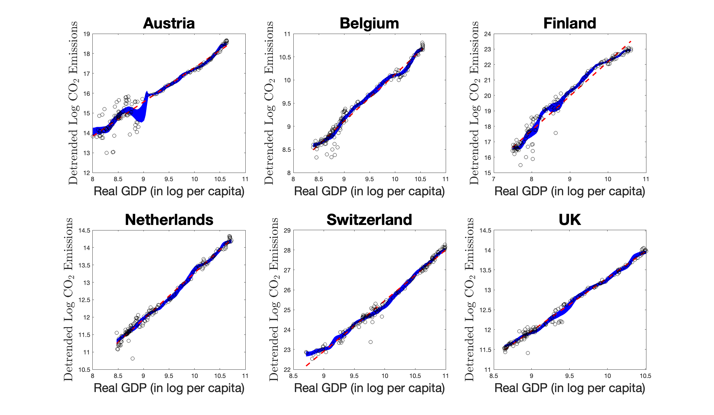
Refer to caption
Figure S12: The 95% (point-wise) confidence intervals of the non-parametric kernel estimate for the relationship between GDP and CO2 emissions (blue) after removal of the country-specific and joint flexible deterministic trends. The red dotted line is the linear fit. Results are based on the full sample.
Refer to caption
Figure S13: The 95% (point-wise) confidence intervals of the non-parametric kernel estimate for the relationship between GDP and CO2 emissions (blue) after removal of the country-specific and joint flexible deterministic trends. The red dotted line is the linear fit. Results are based on observations after World War II.