On the implementation of a global optimization method for mixed-variable problems
Giacomo Nannicini
IBM Quantum, IBM T.J. Watson research center, Yorktown Heights, NY
Abstract
We describe the optimization algorithm implemented in the open-source derivative-free solver RBFOpt. The algorithm is based on the radial basis function method of Gutmann and the metric stochastic response surface method of Regis and Shoemaker. We propose several modifications aimed at generalizing and improving these two algorithms: (i) the use of an extended space to represent categorical variables in unary encoding; (ii) a refinement phase to locally improve a candidate solution; (iii) interpolation models without the unisolvence condition, to both help deal with categorical variables, and initiate the optimization before a uniquely determined model is possible; (iv) a master-worker framework to allow asynchronous objective function evaluations in parallel. Numerical experiments show the effectiveness of these ideas.
1 Introduction
An optimization problem without any structural information on the objective function or the constraints, but for which we have the ability to evaluate them at given points, is called a black-box problem. The area of derivative-free optimization is dedicated to the study of optimization algorithms that do not rely on computing the partial derivatives of the objective function, and it is naturally applied to black-box problems. Many optimization problems in engineering are solved by treating them as a black box, for two main reasons: first, the objective function may not be known in an explicit form, e.g., when it is the output of a complex computer simulation; second, even if derivatives may exist and be computable, the effort required may make it impractical, or the low accuracy of their computation may make them unreliable.
This paper discusses the implementation of a global derivative-free optimization algorithm that is specifically aimed at black-box problems with expensive objective function evaluations. The algorithm accepts as input problems of this form:
| (1) |
where for , is an (unordered) finite set, and are vectors of finite lower and upper bounds. Problem (1) is a mixed-variable problem, because it involves continuous variables, discrete integer variables, and discrete categorical variables (i.e., variables that belong to a finite, not necessarily ordered set). Mixed-variable problems are notoriously difficult to solve, but they have wide-ranging applications, see e.g., [3]. Note that (1) is unconstrained: while constraints greatly increase modeling capabilities, the majority of the derivative-free optimization literature deals with unconstrained problems. This is mainly due to two reasons: first, simple constraints can be incorporated by penalizing their violation in the objective function; second, problem (1) is already difficult to solve, so unless the constraints are relatively easy to handle, complicated (possibly black-box) constraints may make its solution too difficult in practice11 1 For an example of a difficult constrained black-box optimization problem, we refer the interested reader to the MOPTA 08 problem discussed at https://www.miguelanjos.com/jones-benchmark; see also [32]..
Among the numerous methodologies proposed for derivative-free optimization, there is an emerging consensus that algorithms based on surrogate models typically have better global performance on nonconvex problems with continuous variables. A surrogate model is a model of the unknown objective function, that can be used by the optimization algorithm as a proxy to obtain estimates of the objective function value at unseen points in the domain. The algorithm discussed in this paper employs a surrogate model constructed as a weighted combination of radial basis functions (RBFs), plus a polynomial tail. At each iteration, the algorithm uses the surrogate model to determine the next point at which the objective function should be evaluated; this decision is based on criteria first introduced in [16, 33], together with the modifications discussed in [10]. We generalize these approaches in multiple ways, the most notable of which are:
- (i)
We introduce a surrogate model defined in an extended space, mapping categorical variables to their unary encoding, and showing that all steps of the optimization algorithm can be performed in a natural way in either the original or the extended space.
- (ii)
We employ a periodic refinement phase, aimed at improving the best known solution with a local search. The local search consists of a small number of steps of an iterative gradient descent method, based on a linear local model of the objective function.
- (iii)
We do not enforce the unisolvence condition of the surrogate models, to both help with categorical variables (for reasons that will be discussed later), and to be able to start optimizing before a unique surrogate model is available.
- (iv)
We describe a parallel implementation of the algorithm that allows asynchronous, simultaneous objective function evaluations.
The resulting optimization algorithm is implemented in an open-source library called RBFOpt, first introduced in [10]. The paper [10] is based on RBFOpt version 1.0, while this paper discusses innovations introduced between version 1.0 and the current 4.2 version22 2 [10] is based on Gutmann’s RBF method [16], which was the default global search method in RBFOpt before being replaced in version 1.2.. We give a full description of several important implementation details that were not previously discussed. Numerical experiments show the effectiveness of these modifications on a set of nonconvex problems, as compared to the algorithm of [10], and as compared to several open-source derivative-free optimization solvers: NOMAD [20], Nevergrad [30], Optuna[1], Scikit-Optimize [17], SMAC [18]. We provide an example of a typical application by evaluating the performance of RBFOpt for the optimization of the hyperparameters of a random forest classifier on a given dataset. We remark that RBFOpt is designed for deterministic black-box optimization problems, rather than hyperparameter optimization problems where the result of each objective evaluation is typically a sample from a random variable; however, we can use RBFOpt by simply fixing the dataset and the random seed used to train the classifier, thereby making the objective function deterministic. This runs the risk of overfitting, as RBFOpt only observes one realization of a generalization error estimator, but in practice it can be an acceptable tradeoff. Results show that the main innovations discussed above have a significant impact on performance not only on artificial test functions, but also in this specific hyperparameter optimization application33 3 RBFOpt is used in a commercial product to optimize hyperparameters of machine learning models; while our benchmark set contains artificially generated functions, development is largely driven by hyperparameter optimization applications..
The rest of this paper is organized as follows. In Sect. 2 we review RBF interpolation. In Sect. 3 we discuss two natural approaches to incorporate categorical variables into the surrogate model, setting the stage for an optimization algorithm. Sect. 4 describes the optimization algorithm, including several of the main contributions of this paper. Finally, Sect. 5 provides an extensive numerical evaluation of the optimization algorithm, and Sect. 6 concludes the paper.
2 Surrogate models with radial basis functions
Given distinct points , a RBF interpolant to the points is defined as:
| (2) |
where , and is a polynomial of degree . We use subscripts to refer to elements of a vector, and superscripts to denote distinct vectors, e.g., is the -the element of the -th vector of the collection ; the superscripts should not be confused with exponents, because except for Table 1, all polynomials in the rest of the paper do not involve variables — only scalars. Notice that here and in the rest of this paper, for notational convenience we use as a general shorthand for the dimension of the space in which the interpolation points live; the value for is specified in the next section. Furthermore, we remark that here is a generic variable name, and should not be intended to refer only to continuous and integer variables as in (1). The degree of the polynomial is chosen according to Table 1, depending on the type of radial basis functions .
| (linear) | 0 | |
| (cubic) | 1 | |
| (multiquadric) | 0 | |
| (thin plate spline) | 1 | |
| (Gaussian) | -1 |
If is cubic or thin plate spline, we obtain an interpolant of the form:
| (3) |
where . The values of can be determined by solving the following linear system:
| (4) |
with:
If , , and the points are pairwise distinct, then (4) is nonsingular; this is a sufficient but not necessary condition, used by Gutmann’s RBF algorithm [16] to guarantee uniqueness of the interpolant on problems with continuous variables.
3 Optimization with categorical variables in extended space
In the rest of this paper, we assume that for all . For , we define and , with for convenience. We use to denote inner products. Since (1) has categorical variables, which are difficult to handle in any mathematical optimization framework due to their unstructured nature, we work with two inexact formulations for (1). The first formulation, which we call original space formulation, simply replaces the categorical variables with integer variables. Define the vectors as:
Then the original space formulation is defined as:
| (5) |
where is a one-to-one map of the integers to elements of the -dimensional set . Notice that to construct the function , we must arbitrarily define an order of each set . This allows us to apply any algorithm for mixed-integer black-box problems directly to (1). However, it is an inherently flawed approach, because the sets are originally unordered. Since virtually all derivative-free optimization algorithms use metric information, we are imposing on the problem artificial structure that is not reflected in its original formulation.
The second formulation, which we call extended space formulation, uses a unary encoding for the categorical variables. Define the vectors as:
Then the extended space formulation is defined as:
| (6) |
where maps the binary vector to a choice of elements from the sets , by viewing it as the juxtaposition of the characteristic vectors of the sets . This mapping assigns one value to each categorical variable, because of the constraints for all . In the following we denote the feasible region of (6) as . Notice that similar to the previous formulation, (6) also suffers from the flaw of imposing an order on the sets ; however, we show next that a surrogate model of (6) with radial basis functions ignores the order, thereby avoiding ranking points based on artificial metric information (i.e., that does not exist in the original problem).
Proposition 3.1 (Invariance to permutation)
Let with corresponding function values . Let be a permutation of , where for , is a permutation of . Let be the extension of to an operator on -dimensional vectors that acts as the identity on the first components. Let define an interpolant
| (7) |
to the points with values . (If the polynomial tail is of degree according to Table 1, then is the all-zero vector; if the degree is , is 0 as well.) Then for any , the function , defined as:
is such that .
Proof.
Since by definition is a permutation of the components of the vector , and acts as the identity on the first components, we have:
and
This immediately implies . ∎
Prop. 3.1 implies that the surrogate model in extended space is invariant to the order adopted in the unary-encoding representation of the categorical variables. Indeed, if the solution to (4) is unique, yielding a unique surrogate model , after permuting the unary encoding of the categorical variables we would obtain the same surrogate model from (4). We remark that if the solution to (4) is not unique (see Sect. 4.1), then one may obtain a different after permuting the unary encoding of the categorical variables; however, even in this case, each solution to (4) has an equivalent solution for the system obtained after permutation. Note that similar properties do not hold when using the original space formulation: if categorical variables are represented by integers in the interval , permuting these integers is not a component-wise permutation of the vector , and could in general change the norms of .
We can therefore use the extended space formulation (6) together with surrogate models of the form (2) to ensure that the sets are correctly treated as unordered. However, (6) is a constrained formulation, whereas the algorithms of [16] and [33] (that RBFOpt is based on) assume unconstrained problems. In the next sections we describe one way to deal with the constraints in (6). Another difficulty is given by the fact that the constraints lead to linearly dependent columns in the submatrix of (4); this issue is also discussed in the next sections. From now on, we define , i.e., the dimension of the extended space: the interpolation model (2) lives in -dimensional space. Note that we always require the representation of the categorical variables in extended space to take on integer values, as is natural. This is in contrast with popular hyperparameter optimization approaches, where the categorical variables are often treated as continuous for simplicity, and the fractional values are then mapped to a valid discrete value in some heuristic way (such as setting the variable with the largest fractional value to 1, and the rest to 0; this is the approach implemented, e.g., in Spearmint [37]). From an optimization standpoint, it seems more rigorous to treat integer variables as such, because it is well-known that a solution to the relaxed problem could be very far from the integer optimum, even for linear optimization problems [27].
Finally, to better understand the structure of the surrogate model in the extended space, we rewrite it as follows. For , define , i.e., the subvector corresponding to the unary representation of the -th categorical variable. With this definition, note that can be rewritten as:
From the above equation we can see that the argument of the radial basis function centered at the interpolation point is shifted by the number of categorical variables that disagree with . Thus, for the radial basis function part of the interpolant, the surrogate model is determined by the non-categorical variables, as well as the number of disagreements with the categorical variables at the interpolation nodes: the only notion of distance between categorical variables is reduced to the binary information agreement/disagreement, which is independent from the order assigned to the sets . Furthermore, depending on the degree of the polynomial tail, there can be an additional shift of the entire surrogate model that depends only on the values of the categorical variables (i.e., the part corresponding to categorical variables in the inner product term ).
It should be noted that if a categorical variable, say the first categorical variable for simplicity, has only two possible values, i.e., , then the extended space formulation is redundant: the constraint implies that is simply the complement of . As will be discussed in Sect. 4.1, one among would always be eliminated when determining the coefficients of the surrogate model. Hence, we use the extended space formulation only for categorical variables that have strictly more than two possible values: for those that have exactly two, we use the original space formulation, mapping them to a binary variable.
4 Description of the optimization algorithm
Many RBF-based global optimization methods use a similar scheme that attempts to balance exploration (trying to improve a surrogate model of the objective function in unknown parts of the domain) with exploitation (trying to find the best objective function value based on the current surrogate model); see, e.g., [16, 33, 25, 24, 14]. The algorithm that we propose is no exception, although we introduce some additional steps (Refinement step and Restoration step, see below) as compared to the more traditional framework. More specifically, we use the following optimization scheme:
- •
Initial step: Set equal to the size of the initial sample set. Choose affinely independent points using an initialization strategy.
- •
Iteration step: Repeat the following steps until exceeds the prescribed number of function evaluations.
- (i)
Compute the RBF interpolant to the points , solving (4). If the system is not full rank, find the least squares solution. If the system cannot be solved, go to Restoration step.
- (ii)
Choose a trade-off between exploration and exploitation.
- (iii)
Determine the next point based on the choice at step (ii).
- (iv)
Evaluate at .
- (v)
Set . If the last Refinement step was performed sufficiently many iterations ago, go to the Refinement step. Otherwise, repeat the Iteration step.
- (i)
- •
Refinement step:
- (i)
Select points out of to initialize a local model.
- (ii)
Apply a local search method for a specified number of iterations, obtaining points .
- (iii)
Set and go back to the Iteration step.
- (i)
- •
Restoration step: Attempt to change the set of interpolation points so that (4) admits a solution. If successful, return to Iteration step. Otherwise, restart the algorithm.
The algorithm described above can be considered a meta-algorithm, with many possible instantiations. The choice of the initial sample points is discussed in [10]; in this paper we always select them by constructing a latin hypercube design aimed at maximizing the minimum distance between the sample points. In the following, we provide an overview of the main different implementations of the above meta-algorithm available in RBFOpt. We remark that [10] describes several improvements to the meta-algorithm (in the context of Gutmann’s RBF method [16]); all of them are used by default in RBFOpt. Most notably, these are: automatic scaling of the domain of the function; clipping and rescaling of the codomain; restriction of the search box during global search — see [10] for details.
4.1 Solution of linear systems and non-unique interpolants
To compute the surrogate model we must solve system (4). However, when the polynomial is of degree 1, if some of the interpolation points are affinely dependent then (4) has determinant 0. In continuous space, the algorithm never generates affinely dependent points44 4 To be precise, the algorithm only guarantees pairwise distinct points; but the probability of selecting a new point that is affinely spanned by the previous points is with the MSRSM algorithm [33], and only happens in ill-conditioned cases for Gutmann’s algorithm [16].. With categorical variables, this is bound to happen: because of the constraints for all , the binary representation of each categorical variable in extended space adds up to the all-one vector, which is already a column of (4) whenever in Table 1. To solve this issue, whenever the problem has categorical variables and , we eliminate the columns for and the corresponding rows from (4). These are precisely the last columns of each constraint for all . This is motivated by the following simple observation.
Proposition 4.1 (Reduced linear system)
Proof.
Let be a solution to (4). Since for all , we can eliminate from ; if we define as the vector with in the last component and in all other components, the substitution yields:
This shows that is also a solution to (4). However, by definition the -component of is zero, implying that we can eliminate the column corresponding to from (this also eliminates one row from , which obviously does not restrict the set of solutions to the system). We can repeat this process for for , showing that the reduced system admits a solution and completing the proof. ∎
By the above proposition, we can solve (8) rather than (4), find a solution to the smaller system, and extend it to a full solution by inserting zeroes in the positions corresponding to eliminated columns. The advantage of this approach is that (8) may be an invertible system whereas (4) is not invertible under the stated conditions.
Affinely dependent points affect not only the nonsingularity of the system (4), but also the unisolvence property of RBF interpolants, i.e., uniqueness of the interpolant [29]. In particular, when in Table 1, the sufficient condition for unisolvence — using a basis of polynomials of degree 1 — fails because we eliminate one or more monomials from the polynomial basis. Thus, when we can no longer guarantee the unisolvence property. However, in practice we observe that the system (4) often has a solution even when this condition fails, and sometimes a unique solution; this was also observed in [13].
Even when using the reduced matrix , it can sometimes happen that the algorithm generates affinely dependent interpolation points. Specifically, this can occur when there are integer or categorical variables, where column entries belong to a discrete set; empirically, we observe this especially when the problem has many binary variables. When this happens, we solve (8) as a least-squared-residuals problem. This is computationally more expensive, but guarantees a solution. (The time spent in the solution of linear systems is negligible in practice.)
The least squares solution to the linear system is also used whenever there are not enough sample points to build a full interpolant, i.e., . Whereas the majority of the literature assumes that at least points are sampled in the initialization phase (see, e.g., [16, 33, 10]), in practice this can be a severe drawback when is large. Approaches to begin the optimization before sampling points are described in [31, 34]; we follow the approach of [34]55 5 The numerical tests in [34] are based on a customized version of RBFOpt.. Specifically, the number of initial sample points is heuristically chosen according to the following formula:
| (9) |
If RBFOpt is executed in parallel with at least 2 threads, then the number of initial sample points is chosen as:
As long as , we use the least squares solution to determine the coefficients of the surrogate model ; the rest of the optimization algorithm remains unchanged. Whenever points are available and they are affinely independent, system (4) has a unique solution and we compute it using a direct method.
The reduced matrix is also employed in the Initial step of the algorithm. After generating an initial sample set (see [10] for a description of the strategies to do so implemented in RBFOpt), we compute a singular value decomposition of ; as long as some singular value is close to zero, we generate a new sample set. Notice that if there are no categorical variables then coincides with .
We remark that for all RBFs that do not have a polynomial tail of degree 1, i.e., all except the cubic and thin plate splines, these additional steps are not necessary. However, the cubic and thin plate spline RBFs are empirically among the most accurate, see e.g. [10], and the automatic model selection procedure employed by RBFOpt (see Sect. 4.5) chooses one of these two RBFs very often in practice. Hence, the additional effort is justified.
4.2 Determining the next point: Iteration step
We implement a variation of two algorithms for global optimization using RBFs: Gutmann’s RBF algorithm [16] and the Metric Stochastic Response Surface Method (MSRSM) [33]. Both algorithms proceed in cycles, and use a parameter that determines the length of an optimization cycle.
4.2.1 Gutmann’s RBF algorithm
A detailed description is given in [10]; here we report the main steps only. Let be the RBF interpolant to the points , with function values respectively. Let be the coefficient of corresponding to the RBF centered at . Define
where is a given value. Furthermore, define:
| (10) |
Gutmann’s RBF method then implements the following Iteration step:
- •
Iteration step (for Gutmann’s RBF algorithm):
- (ii)
Choose a target value .
- (iii)
- (ii)
Let , , and . We employ a cyclic strategy that picks target values according to the following sequence of length :
- •
Step (InfStep): Choose . In this case the problem of finding can be rewritten as:
This is a pure exploration phase, yielding a point far from .
- •
Step (Global search): Choose
(12) In this case, we try to strike a balance between improving model quality and finding the minimum.
- •
4.2.2 MSRSM algorithm
Define . The MSRSM algorithm implements the following Iteration step:
- •
Iteration step (for the MSRSM algorithm):
- (ii)
Choose a target value .
- (iii)
Choose a finite set of reference points , and compute
(13)
- (ii)
Essentially, (13) tries to solve a bi-objective optimization problem in which the two objective functions are the (negative of the) maximin distance from the points , and the value of the surrogate model. The paper [33] uses a variation of (13), in which the second fraction in the expression has weight rather than . RBFOpt supports this version, but by default it uses equation (13) instead (see also [9]).
The value of is chosen according to a cyclic strategy of length in which each step has similar goals to the corresponding step discussed in Gutmann’s RBF method. The cyclic strategy is as follows:
- •
Step (InfStep): Choose . In this case the problem of finding can be rewritten as:
This is a pure exploration phase.
- •
Step (Global search): Choose . This aims for balance between exploration and exploitation.
- •
Step (Local search): Choose . In this case, the solution to (13) is the point that minimizes the surrogate model, i.e., . If is such that , we accept as the new point . Otherwise, choose . This is an exploitation phase.
4.2.3 Solution of the search problems
We implement three different approaches for the solution of the optimization problems (11) and (13):
- (1)
Problems (11) and (13) are solved with a simple genetic algorithm, that works by generating an initial population uniformly at random, then iteratively constructing a new population by taking:
- •
The best points in (surviving population), according to the objective function being optimized;
- •
points obtained by repeatedly performing the following procedure: we randomly pick two points from the surviving population, and create a new point by choosing each entry from either or (mating);
- •
points generated uniformly at random (new individuals);
- •
a point obtained by taking the best individual in , and randomly perturbing some of its entries (mutation). The number of mutated entries increases as the number of iterations of the genetic algorithm increases.
We appropriately round the above quantities so that the size of the population remains constant. In the presence of categorical variables we sample points in the original space, where uniform random sampling is easily implemented, then map them to the extended space.
- •
- (2)
Rather than solving (11) and (13) directly, we sample a large number of points in and choose the best point in the sample. This is the approach advocated in [33]. In the presence of categorical variables we sample points in the original space, where uniform random sampling is easily implemented, then map them to the extended space.
- (3)
Problems (11) and (13) are solved by means of the mathematical programming solvers Ipopt and Bonmin. This is the approach advocated in [16]. Since Bonmin supports constrained problems, we work directly in the extended space when this approach is chosen (note that we must use Bonmin if discrete variables are present).
We remark that the MSRSM scoring function requires a set of reference points , see (13): the set of reference points is taken to be the current population for the genetic algorithm, the whole sample when using the sampling scheme, and for when using a mathematical programming solver.
4.3 Determining the next point: Refinement step
As indicated at the beginning of Sect. 4, during the search we periodically execute a Refinement step, with the purpose of improving the best solution available by performing a local search around it. The scheme employed in the Refinement step is reminiscent of a trust region method [6, 39]. However, it is not a trust region method, mainly because we construct a local model using points that may be outside the trust region, and we do not require that the model is fully-linear or a similar property [8] (although the QR-like algorithm that we use to improve the geometry of the interpolation set would in principle yield a fully-linear model, if it were allowed to run to completion [39, 7]). Furthermore, our scheme is adapted to work on mixed-variable problems, rather than only problems with continuous variables; proving rigorous local convergence guarantees in the discrete setting is an involved task in itself, see e.g., [21], and here we limit ourselves to a heuristic approach to refine candidate solutions. While trust region methods enjoy strong convergence properties [8], managing the set of sample points and converging to a stationary point can be expensive, compared to surrogate model methods, in terms of number of objective function evaluations. Empirically, we found that embedding a full trust region method for local search could severely slow the global search, which is the main strength of RBF-based surrogate model methods; hence, we opted for the methodology described below, that is guided by two design priciples: (1) it is initialized using information from known points only; (2) it is quickly stopped if it fails to yield any improvement. Note that with our approach the RBF surrogate model is still used for global and local search, but it is complemented by a local linear model to search around the best known solution; this is contrast to the approach recently proposed in [15], where the global surrogate model is abandoned altogether, and is replaced by multiple local models managed with a trust-region-like algorithm.
We define the following algorithmic parameters, utilized in the algorithm.
- •
: minimum radius of the refinement search.
- •
: (logarithm of the) radius multiplier for initialization.
- •
: threshold to shrink the refinement search radius.
- •
: threshold to expand the refinement search radius.
- •
: threshold to accept the new iterate.
- •
: frequency parameter of the refinement search.
- •
: maximum number of consecutive refinement iterations.
- •
: minimum norm of the gradient of the linear model.
The Refinement step works as follows:
- •
Model initialization: Let . Sort the points by increasing distance from , and select the first (this includes itself). Let be the set containing these points. Set .
- •
Let be the point in with the smallest distance to . Compute the initial radius of the refinement search as:
- •
Refinement: repeat a given number of times, or until a stopping criterion is met.
- (i)
Let be the matrix obtained using the points as columns.
- (ii)
If does not contain affinely independent columns, use a factorization of to replace one point in with a new point (obtained by moving from in a direction taken from the columns of after rescaling, with step length ) that increases the rank of , and go back to (i).
- (iii)
Otherwise, build a linear model of the objective function using points .
- (iv)
Move from the current iterate in the direction of improvement with step length:
Let be the new candidate point.
- (v)
Evaluate . Update the refinement search radius based on the expected decrease and the actual decrease : if , set , if set .
- (vi)
If , set .
- (vii)
Replace the point in furthest from with the new point , if it is closer, and go back to (i).
- (i)
The Refinement step is triggered after full cycles of the global search strategy in the Iteration step (i.e., the strategy to select in Gutmann’s RBF method, or in MSRSM), but only if one of the following two conditions apply: (i) a better solution was discovered since the last execution of the Refinement step, or (ii) the last Refinement step was stopped because of its iteration limit (parameter , see below), rather than for lack of improvement.
When the Refinement step ends, all points at which has been evaluated are added to , and the algorithm goes back to the Iteration step. The Refinement step ends when one of the following conditions is verified:
- •
after consecutive iterations, unless we are close to hitting the limit on the maximum number of objective function evaluations, or the CPU time limit (this is defined by a further parameter);
- •
if the radius of the refinement search drops below ;
- •
if the norm of the gradient of the linear model drops below .
The above scheme is designed with continuous variables in mind, but we heuristically apply the Refinement step also in the presence of integer or categorical variables. When the problem has integer or categorical variables, the Refinement step proceeds as described above, but every candidate point is rounded to an integer point before being evaluated with . In particular, every integer variable that takes on a fractional value in the candidate point, say , is rounded down with probability , and rounded up with probability ; whereas every unary representation of a categorical variable, say such that in extended space, is rounded to the orthonormal basis vector with probability for all . The rounding process for integer and categorical variable is repeated a given number times, and the point with the best linear model score is chosen as the next candidate. A similar procedure is applied in step (ii) to the column of that is about to replace one column in : each entry is projected to the closest feasible vector in extended space, using -norm distance.
4.4 Repairing numerical errors: Restoration step
Whenever numerical errors are detected in the solution of the linear system (4), we switch to a Restoration step that works as follows. Given the list of interpolation points , for we heuristically solve the problem:
then temporarily replace with the solution to the above problem, say . If the system (8) for the points is invertible, we permanently replace with , and the Restoration step is successful. Otherwise, we reinstate and continue the Restoration step by decreasing . We remark that several interpolation points may be added in between successive solutions of (4), because the Refinement step may perform multiple iterations and it does not recompute the interpolant . For this reason, we cannot hope that removing the last interpolation node is always sufficient to fix numerical errors.
The rationale for solving a maxmin distance problem when trying to improve the numerics is that proximity to other interpolation points necessarily leads to an ill-conditioned linear system: if two points are very close to each other, the corresponding rows in (4) are almost identical. This suggests maximizing the distance from other interpolation points as the main criterion for choosing a point. Furthermore, this criterion corresponds to the “pure exploration” phase of the MSRSM algorithm, trying to gather information in unexplored parts of the search space; hence, it naturally fits into our optimization scheme.
4.5 Automatic model selection
In order to dynamically choose the surrogate model that appears to be the most accurate for the problem at hand, we assesses model quality using a cross validation scheme. This was introduced in [10]: here we give a brief summary of the main ideas, and report some additional implementation details introduced subsequently.
Suppose we have interpolation points with surrogate model . We assume that the points are sorted by increasing function value: ; this is without loss of generality as we can always rearrange the points. We perform cross validation as follows. For , we fit a surrogate model to the points for and evaluate the performance of at . We use an order-based measure to evaluate performance of the surrogate model. For a given scalar , let be the position at which should be inserted in the ordered list to keep it sorted. Since , we use the value to assess the predictive power of the model. We then average with ranging over some subset of to compute a model quality score. This approach is a variation of leave-one-out cross validation in which we look at how the surrogate model ranks the left-out point compared to the other points, rather than evaluating the accuracy of the prediction in absolute terms. This is motivated by the observation that for the purpose of optimization, a surrogate model that ranks all points correctly is arguably more useful than a surrogate model that attains small absolute errors, but is not able to predict how points compare to each other [4].
We perform model selection at the beginning of every cycle of the search strategy to select or (depending on the choice of algorithm: Gutmann’s RBF or MSRSM). Our aim is to select the RBF model with the best predictive power. We choose two different models: one for local search, one for global search, corresponding to different Iteration steps of the algorithm. We do this by computing the average value of for , and the average value of for .
The RBF model with the lowest value of is employed in the subsequent optimization cycle for the Local search step and the Global search step with , while the RBF model with lowest value of is employed for all the remaining steps. We consider all RBFs listed in Table 1. This implies that the type of RBF dynamically changes during the course of the optimization.
In [10], we show that the values can be computed in time , where is the number of rows of (4) (i.e., for cubic and thin plate spline RBF, for linear and multiquadric, for Gaussian). This is achieved by reusing the same LU factorization of the system (4) for each iteration of the cross validation routine. Details of this approach are given in [10].
When automatic model selection is enabled, we build the surrogate model using thin plate splines until there are enough points to start the automatic model selection procedure. Furthermore, after executions of the automatic model selection procedure, where is a parameter, we trust the results obtained up to that point and use the type of RBFs that gave the smallest error the largest number of times. Results for the local search model and global search model are kept separate. In other words, the quantities and are computed at most times; after that, we always use the RBF type that gave the smallest value of the largest number of times out of for local search, and similarly with for global search. This can lead to large time savings on problems with several thousand interpolation points, as leave-one-out can become expensive if it has to perform thousands of iterations with a large system (4).
4.6 Parallel optimizer
Our implementation supports asynchronous parallel evaluation of the objective function , which is assumed to be the most time-consuming part of the optimization process. The parallel optimization algorithm is nondeterministic due to its asynchronous nature. This algorithm was first introduced in [11]; here we give a brief overview, as well as several implementation details that were not present in the version of [11].
The parallel optimizer works by creating a set of worker threads, coordinated by a master. The worker threads perform tasks of two types: Type 1 is the evaluation of the objective function at a given point (which is assumed to be time-consuming), Type 2 is the computation of a point at which the objective function should be evaluated (which usually takes only a fraction of a second, but may take longer especially when some subproblems are solved with Bonmin). We always dedicate one worker to perform tasks of Type 1 or of Type 2 related to the Refinement step; however, there is a global limit to the fraction of Refinement steps that can be performed as compared to the total number of iterations. The remaining workers are utilized for the Iteration step. As long as there are available processors, the master removes a task from the queue of active tasks, and assigns it to a worker. Tasks of Type 1 have priority over Type 2, due to their longer execution times. Within tasks of the same type, a first come, first served policy is used.
Recall that to compute the surrogate model we need pairwise distinct points (possibly affinely independent, depending on the degree of the polynomial tail). To ensure that the same point is not evaluated twice in parallel, whenever a task of Type 2 is completed, by determining a point at which should be evaluated next, we add a temporary interpolation point at , with value . This point is converted to a regular interpolation point when the corresponding objective function evaluation (task of Type 1) is complete, and it is assigned its true function value .
For the Refinement step, a new sample set for the linear model is computed from scratch every time that a point with better objective function value is discovered outside the Refinement step; this is different from the serial optimization algorithm, where the Refinement step is executed in consecutive iterations and no such event can occur. Another major difference in the parallel optimizer is that we do not perform the Restoration step: when (4) cannot be solved and the queue of active tasks is empty, we restart the algorithm. (If the queue is not empty, the algorithm keeps processing tasks that have finished until (4) can be solved, or the queue is empty.) The choice to restart, rather than attempt a Restoration step, has several motivations. The main reason is that removing an interpolation node requires synchronizing all threads to ensure exclusive access to the relevant data structures; because function evaluations can be very time-consuming, this may leave several threads idle for a long time. Another reason is that, since multiple point evaluations are performed in parallel, it is possible that other points in the queue lead to numerical instability: the Restoration step would have to eliminate all of them, potentially provoking a prolonged period of inefficient CPU use. Finally, the Restoration step is not guaranteed to work unless we allow removing multiple points from the set 66 6 This is also the case for serial (i.e., non parallel) optimization, but in the serial case removing the most recent interpolation point yields an invertible system (4) in all cases except when multiple points are added in consecutive Refinement steps.; however, choosing a subset of points to remove is a difficult combinatorial problem, hence we opt for a simpler approach.
5 Computational experiments
RBFOpt is implemented in Python and available on GitHub; it can be automatically installed from PyPI using pip. In this section we evaluate the computational performance of the solver, with a focus on testing the features of the optimization algorithm described in Sect. 4. All experiments are run on identical virtual machines with (virtual) Intel Xeon E5-2683 v4 CPUs, clocked at 2.10GHz and running Linux; these machines are instantiated on an IBM cloud. We use Ipopt [38] and Bonmin [5] to solve all auxiliary subproblems that require a mathematical programming solver (Bonmin is used only if the subproblem has integer variables). Note that these subproblems are not necessarily solved to optimality, as they are generally nonconvex (e.g., minimizing the surrogate model or solving (11)); we put a time limit of 20 seconds on each execution of the solvers, and Bonmin is configured with the “B-BB” algorithm.
5.1 Test instances
We test the algorithm on a set of 54 instances, with the following characteristics:
- •
22 instances have continuous variables only, but no integer or categorical variables;
- •
20 instances have integer variables only, or continuous and integer variables, but no categorical variables;
- •
12 instances have any combination of variable types and have at least one categorical variable.
In Table 2 we give details on the number of variables and the source of each problem. All these problems are highly nonconvex, and their dimension is relatively small. The instances with categorical variables are obtained by modifying other problem instances, easily identified by their names. The categorical variables determine one or both of the following: (1) they modify some of the problem’s data, i.e., vectors of coefficients that appear in the cost function; (2) they modify some of the functions involved in the expression for the objective function, although they do not modify their arguments (e.g., the objective function contains an expression , and one of the categorical variables determines what function is used among a finite set). All categorical variables in our set of test problems have at least three possible values, since, as already mentioned, categorical variables with only two possible values are modeled as binary variables.
| Instance | # variables | Source | Instance | # variables | Source | ||||
|---|---|---|---|---|---|---|---|---|---|
| Cont. | Int. | Cat. | Cont. | Int. | Cat. | ||||
| branin | 2 | 0 | 0 | S1 | nvs06 | 0 | 2 | 0 | S3 |
| camel | 2 | 0 | 0 | S1 | nvs07 | 0 | 3 | 0 | S3 |
| ex4_1_1 | 1 | 0 | 0 | S2 | nvs09 | 0 | 10 | 0 | S3 |
| ex4_1_2 | 1 | 0 | 0 | S2 | nvs14 | 0 | 5 | 0 | S3 |
| ex8_1_1 | 2 | 0 | 0 | S2 | nvs15 | 0 | 3 | 0 | S3 |
| ex8_1_4 | 2 | 0 | 0 | S2 | nvs16 | 0 | 2 | 0 | S3 |
| goldsteinprice | 2 | 0 | 0 | S1 | prob03 | 0 | 2 | 0 | S3 |
| hartman3 | 3 | 0 | 0 | S1 | schoen_6_1_int | 2 | 4 | 0 | S6 |
| hartman6 | 6 | 0 | 0 | S1 | schoen_6_2_int | 2 | 4 | 0 | S6 |
| least | 3 | 0 | 0 | S2 | schoen_10_1_int | 4 | 6 | 0 | S6 |
| perm_6 | 6 | 0 | 0 | S5 | schoen_10_2_int | 4 | 6 | 0 | S6 |
| perm0_8 | 8 | 0 | 0 | S5 | sporttournament06 | 0 | 15 | 0 | S3 |
| rbrock | 2 | 0 | 0 | S2 | st_miqp1 | 0 | 5 | 0 | S3 |
| schaeffer_f7_12_1 | 12 | 0 | 0 | S4 | st_miqp3 | 0 | 2 | 0 | S3 |
| schaeffer_f7_12_2 | 12 | 0 | 0 | S4 | st_test1 | 0 | 5 | 0 | S3 |
| schoen_6_1 | 6 | 0 | 0 | S6 | branin_cat | 2 | 0 | 1 | – |
| schoen_6_2 | 6 | 0 | 0 | S6 | ex8_1_1_cat | 2 | 0 | 2 | – |
| schoen_10_1 | 10 | 0 | 0 | S6 | hartman3_cat | 3 | 0 | 1 | – |
| schoen_10_2 | 10 | 0 | 0 | S6 | hartman6_cat | 6 | 0 | 1 | – |
| shekel10 | 4 | 0 | 0 | S1 | schoen_10_1_cat | 10 | 0 | 2 | – |
| shekel5 | 4 | 0 | 0 | S1 | schoen_10_2_cat | 10 | 0 | 2 | – |
| shekel7 | 4 | 0 | 0 | S1 | gear4_cat | 1 | 4 | 1 | – |
| gear | 0 | 4 | 0 | S3 | nvs07_cat | 0 | 3 | 1 | – |
| gear4 | 1 | 4 | 0 | S3 | nvs09_cat | 0 | 10 | 1 | – |
| nvs02 | 0 | 5 | 0 | S3 | st_miqp1_cat | 0 | 5 | 1 | – |
| nvs03 | 0 | 2 | 0 | S3 | schaeffer_f7_12_1_int_cat | 9 | 3 | 1 | – |
| nvs04 | 0 | 2 | 0 | S3 | schaeffer_f7_12_2_int_cat | 9 | 3 | 1 | – |
We also use a randomized procedure to create larger instances starting from a base instance, multiplying its dimension by a given positive integer number. We now give a high-level description of this procedure; full details can be found in the publicly available source code, as a precise description is tedious and does not add further insight. Let be the number of variables of the base instance with objective function , and the size multiplier. The objective function of the enlarged instance is:
where is a partition of the set , the coefficients are randomly chosen within a specified range, for all , , and the are affine functions that map their argument to the original domain of . In other words, the enlarged objective function is the sum of several copies of defined on disjoint sets of variables, with a copy of that acts on linear combinations of all the variables. By construction, the value of the optimum stays the same as in the base instance. We finally permute all the variables in the enlarged instance. Notice that we do not change the variable type; e.g., if the base instance has continuous variables and categorical variables, using dimension multiplier yields an instance with continuous variables and categorical variables. From an empirical evaluation, the enlarged instances are much more difficult than the base instances; this is likely due to the final copy of that acts on linear combinations of variables, thus creating interactions between decision variables that may not have been present in the original instance. Our final test set consists of all instances listed in Table 2, plus all instances obtained with the above procedure with a size multiplier . This yields 108 problem instances, with a number of variables varying from 1 to 30.
5.2 Comparison of algorithmic variants
To compare algorithmic variants of RBFOpt, we plot performance and data profiles [23], which are defined as follows. Define the budget for an algorithm as the maximum number of function evaluations allowed. Unless specified otherwise, in our experiments the budget is set to . For a given instance and a set of algorithms , let be the best function value discovered by any algorithm, and the first point evaluated by each algorithm, which we impose to be the same. Let be a tolerance. We say that an algorithm solves an instance up to tolerance if it returns a point such that:
| (14) |
and the algorithm fails otherwise. In other words, the algorithm has to close at least of the gap between the initial point and the best point found by any algorithm.
Let be the set of problem instances in the test set. Let be the number of function evaluations required by algorithm to solve problem ( if algorithm fails on problem according to the convergence criterion (14)), and the number of variables of problem . The data profile for an algorithm is the fraction of problems that are solved within budget , defined as:
The performance ratio of algorithm on problem is defined as:
According to this definition, the performance ratio is for the best performing algorithm on a problem instance. The performance profile of algorithm is defined as the fraction of problems where the performance ratio is at most , defined as:


For each of the 108 problem instances, we test 20 different random seeds. All tested variants are given the same sequence of random seeds. We remark that if two variants of the algorithm use the same number of points in the initialization phase and have the same random seed, then they will generate exactly the same initial sample set. For every instance, we aggregate the 20 different random seeds by taking the median objective function value at every iteration; the performance and data profiles are constructed using the aggregate data. In this section we use the serial version of the optimization algorithm.
In our first set of experiments we compare the two methodologies for the Iteration step discussed in Sect. 4.2 (i.e., Gutmann’s method and MSRSM), combined with the three approaches to solve the resulting subproblems discussed in Sect. 4.2.3: the genetic algorithm, the sampling method, and the mathematical optimization solver. We remark that the mathematical optimization solvers are relatively slow, taking up to 20 seconds per solve on the more difficult problems, whereas the genetic algorithm and the sampling method only require a fraction of a second due to their heuristic nature. For this set of experiments only, we parametrize the genetic algorithm and the sampling method in a search-intensive fashion, increasing the number of sampled points and the number of iterations of the genetic algorithm compared to their default values (the genetic algorithm uses a base population size of points and performs iterations, compared to a default of and iterations, while the sampling algorithm samples points, compared to a default of ). All the other parameters for the algorithm are left to their default values. We also remark that the implementation of the MSRSM method with mathematical optimization solvers is not competitive with the other variants, because the solution of (13) with a solver for convex problems is essentially hopeless: the expression of the maxmin distance is highly nonconvex and solvers have a very high chance of getting trapped in poor local minima. Hence, we only report results for five algorithmic variants: all combinations of Gutmann’s method and MSRSM with the genetic algorithm, the sampling approach, and the mathematical optimization solver approach, minus the combination MSRSM + mathematical optimization solver. Results are plotted in Fig. 1. The plots quite convincingly show that the genetic algorithm is overall the best choice, with both Gutmann’s method and MSRSM. The sampling method has a similar performance, while using the mathematical optimization solver is considerably worse. We attribute this to the fact that the subproblems involved in the Iteration step are hard nonconvex problems, and the solvers are likely to struggle. (We remark that the minimization of the surrogate model is always performed using Ipopt or Bonmin, regardless of the methodology used to solve subproblems in the Iteration step.) The difference between Gutmann’s method and MSRSM is small, but MSRSM emerges as the winner by a small margin. In the following, we use MSRSM with the genetic algorithm as the default settings. An important conclusion of our numerical study is the fact that neither method dominates the other: while MSRSM seems slightly better and enjoys the benefit of being conceptually simpler, our plots indicate that Gutmann’s method is competitive.


In the second set of experiments we analyze the impact of the number of sample points for the Initialization step of the algorithm. As discussed in Sect. 4.1, we allow building a surrogate model with less than points, in which case the system (4) may have multiple solutions. In Fig. 2 we report results when using sample points to initialize , as well as the number of points defined in (9), labeled “Default” in the plots. We can see that , and “Default” have the best performance with , and there is no winner among these three. For , the curve for “Default” is not visible in Fig. 2(c) because it is hidden behind the curve for : this is expected, since by equation (9), “Default” uses on most problem instances. Choosing emerges as the winner in these tests, followed by and “Default”, which are indistinguishable on this set of test problems. The motivation for the “Default” setting, which seems slightly inferior to in these tests, is robustness: using a very small number of sample points can increase the variance of the algorithm, hence we prefer the safer setting.


In the last set of experiments for this section, we look at the impact of the Refinement step. Plots are reported in Fig. 3. We compare RBFOpt without the Refinement step, with three versions of the algorithm that employ the Refinement step at different frequencies. Here the results are very clear: the Refinement step significantly improves the performance of the algorithm on this set of instances. The plots suggest that running the Refinement step as frequently as possible is a good idea. A head-to-head comparison77 7 It is known that performance profiles depend on the entire set of algorithms evaluated; therefore, pairwise comparisons can sometimes yield useful information. between the algorithm with Refinement step frequencies of 1 and 3 reveals that the difference is quite small and not as one-sided as it would appear from Fig. 3, see Fig. 4 (results for are essentially identical to those for ). We set the Refinement frequency to 3 as the default value, mostly based on empirical evaluation on applications outside the benchmark set reported here.


5.3 Categorical variables: original versus extended space
In this section we analyze the performance of the optimization algorithm with the two different representations for categorical variables discussed in Sect. 3. We use the same approach as in the previous section; all algorithm parameters are set to their default values indicated in the previous section. For this set of experiments we use the problem instances with categorical variables only, see Table 2, as well as their enlarged version with dimension multiplier . To reduce variance, we use the same points for the Initialization step, regardless of the choice of extended or original space. This is accomplished as follows: for every instance and every random seed, we generate the initial samples in extended space (the number of samples is chosen according to (9)); we then map these points to their equivalent in the original space, and use them to initialize the optimization in original space. As a consequence, the optimization in original space uses more initial samples than it normally would. Results are reported in Fig. 5.


The plots for indicate a clear superiority for optimization in extended space; with the difference is not so clear, with the extended space formulation showing better performance on some instances that can be solved quickly, but the original space formulation converges on more instances in the long run. A possible explanation for this behavior is the fact that the optimization algorithm is quite robust to innaccuracies in the surrogate model (because it favors points with large distance from those already evaluated, and it performs local search around the best known point), hence no reasonable formulation for the categorical variables will perform too poorly. We also remark that with (not reported here), the plots are similar to , but the difference is less pronounced. Overall, the extended space formulation is to be preferred: it manages to close of the gap on all test problems (as indicated by the plots for ), and for almost all problems, it does so very quickly; in the long run the original space formulation solves a few more instances to high precision, but this does not seem enough to offset the advantage of the extended space formulation in the initial iterations.
To compare the original and extended space formulations from a different angle, we also set up an experiment to assess the usefulness of the surrogate models constructed in these two spaces. This is accomplished as follows. For every function with categorical variables in Table 2, we generate an initial sample of points, with . These points are generated as a latin hypercube design maximizing the minimum distance between points, and they are generated in extended space. We then construct a surrogate model interpolating at these points, generate 20000 additional random points in the domain of the function, and rank these 20000 points using the surrogate model. More precisely, assume w.l.o.g. (up to reordering) that the interpolation points are sorted by increasing function value, i.e., ; for every point we infer its position in the sorted list by using its surrogate model value . We then compare this number with the true position of in the sorted list, and record the absolute value of the difference between the two numbers. This is a measure of how well the surrogate model is able to rank unseen points as compared to the known interpolation points. We record the average and standard deviation of the difference over the 20000 randomly generated points. The same procedure is repeated in the original space, using exactly the same points mapped from the extended space. The results are reported in Table 3.
| points | points | points | points | |||||
|---|---|---|---|---|---|---|---|---|
| RBF type | Original | Extended | Original | Extended | Original | Extended | Original | Extended |
| Cubic | 4.1 (1.8) | 4.2 (1.9) | 15.7 (8.0) | 14.3 (8.2) | 28.8 (16.2) | 25.4 (15.9) | 120.5 (83.5) | 102.9 (80.1) |
| Gaussian | 4.8 (2.3) | 4.5 (2.4) | 20.9 (11.9) | 20.2 (12.3) | 39.5 (25.2) | 38.1 (25.9) | 193.1 (131.8) | 186.7 (133.6) |
| Linear | 3.5 (1.4) | 3.3 (1.3) | 15.2 (7.9) | 14.7 (7.7) | 27.1 (15.1) | 25.5 (14.5) | 119.1 (81.5) | 107.6 (78.2) |
| Multiquad. | 3.4 (1.4) | 3.3 (1.3) | 15.4 (8.0) | 14.5 (7.7) | 27.0 (15.2) | 25.4 (14.6) | 118.1 (82.4) | 107.6 (79.0) |
| Thin pl. sp. | 4.1 (1.8) | 4.2 (1.9) | 15.4 (8.0) | 13.9 (8.0) | 28.1 (16.2) | 25.0 (15.9) | 117.6 (82.1) | 101.7 (77.9) |
Even though the standard deviations are fairly high, the averages indicate that the extended space formulation is able to better predict the rank of unseen points. Indeed, the average rank errors are smaller for the extended space model in 18 out of the 20 cases reported in Table 3, and the only two cases in which the extended space has higher average error are recorded when the number of interpolation points is small (), so that the differences between extended and original space are small in the absolute sense. For a larger number of interpolation points, the surrogate model in extended space is consistently better. This, together with the previous set of experiments, and the theoretical justification given in Sect. 3, gives a strong indication of the benefits of our choice.
5.4 Comparison with existing open-source derivative-free solvers
We compare the performance of RBFOpt, parametrized according to the results discussed in previous sections, with several derivative-free solvers that support categorical variables, namely:
- •
- •
- •
Optuna [1] version 2.3.0, a hyperparameter optimization algorithm that uses a tree-structured Parzen estimator to deal with categorical variables.
- •
Scikit-Optimize [17] version 0.8.1, a Bayesian optimization algorithm using Gaussian processes (using the function gp_minimize).
- •
SMAC (sequential model-based algorithm configuration) [18] version 0.13.1, another Bayesian optimization algorithm using Gaussian processes88 8 We used the SMAC4BO interface; at the time of writing this paper, the other interfaces did not work in the available beta version of the software package..
This selection covers the most popular methodologies for derivative-free optimization with categorical variables. We remark that in the above list, only NOMAD is developed for derivative-free optimization in the traditional sense, whereas the other software target hyperparameter optimization problems, which generally have added complications (e.g., the objective function evaluation are nondeterministic, and there may be complicated constraints involving the categorical variables); nonetheless, all these algorithms can be applied to black-box optimization problems with categorical variables (a comparison on a hyperparameter optimization problem is given in Sect. 5.6). All algorithms except NOMAD provide a Python library (NOMAD’s Python library does not support categorical variables).


We report performance and data profiles in Fig. 6. Several remarks are in order to clarify the experimental setup of this section. First, we try to initialize each algorithm with the same set of points to reduce variance: RBFOpt, Nevergrad, Scikit-Optimize are initialized with the experimental design generated by RBFOpt, NOMAD is initialized with the best point in the experimental design generated by RBFOpt, while Optuna and SMAC use their own initialization procedures. Second, due to resource constraints we impose a limit of 3 hours of CPU time for each problem instance; the only two algorithms that hit the time limit are Scikit-Optimize and SMAC, most likely due to the optimization of the expected improvement criterion, whereas all other algorithms are considerably faster (e.g., RBFOpt takes on average 5 minutes per instance, Scikit-Optimize almost 2 hours on average). More precisely, Scikit-Optimize times out on 1053 instances, whereas SMAC times out on 1720 instances, out of 2160. Since we observed cases where Scikit-Optimize and SMAC take more than a day to hit the function evaluation limit, the time limit is necessary to conclude the experimental evaluation within a reasonable time frame. We remark that the slow down when the number of variables or the function evaluation budget are large is a known limitation of Bayesian optimization methods [15]. Despite hitting the time limit, the performance of Scikit-Optimize and SMAC is comparable to that of the other hyperparameter optimization algorithms, because the slow down only occurs after a few hundred function evaluations (the evaluation limit is often ), which is sufficient for them to find a good solution.
Fig. 6 shows that on this set of test instances, the comparison is heavily in favor of RBFOpt. NOMAD is the second best solver, but RBFOpt performs better by a noticeable margin; SMAC is fairly close to NOMAD for , whereas all remaining algorithms are far from achieving the same performance level as the top solvers.
5.5 Parallel optimization
To assess the performance of the parallel version of the optimization algorithm, we modify our test functions so that each objective function evaluation waits for seconds, where is a random variable, before returning a value. Thus, we simulate the effects of a time-consuming objective function oracle. We test two possible distributions for , both of which are log-normal: in the first case is distributed as , where is the normal distribution with mean and standard deviation ; in the second case is distributed as . In both cases we truncate the distributions at 300 seconds, i.e., each objective function evaluation takes at most 300 seconds. Notice that the expected value of the first distribution is (seconds), the expected value of the second distribution is . We denote the first case as the “Faster evaluation” set, the second case as the “Slower evaluation” set. We use the same budget of function evaluations, and run the algorithm with 1, 2, 4, 8 or 16 CPUs99 9 Although it may seem natural to set a function evaluation budget that depends on the number of parallel threads, we use a fix budget for practical reasons: with 108 problem instances, 20 random seeds for each instance, a budget of evaluations, at approximately 1 minute per function evaluation these experiments already take more than one year of CPU time.. To assess the speedup achieved by the parallel algorithm, we report the wall-clock time to converge within of the optimal solution. Notice that the larger the number of CPUs, the faster the evaluation budget is depleted; since the parallel algorithm is unlikely to be as efficient as the serial version, as the number of CPUs increases we expect to converge on a smaller number of instances. Thus, when reporting the average time to convergence we only consider instances and random seeds for which all the variants analyzed in this comparison determine the optimum (up to the specified tolerance). Additionally, we report the number of instances of which convergence to the specified tolerance is attained. The data is reported in Table 4; we use shifted geometric means for the wall-clock times, defined as for a set of values . In total, there are 568 combinations of instances and random seeds for which all variants converge on the “Faster evaluation” set, and 550 on the “Slower evaluation” set.
| Num | Faster evaluation ( sec) | Slower evaluation ( sec) | ||||
| CPUs | Time | Speedup | # conv. | Time | Speedup | # conv. |
| 1 | 797.0 | 1.00 | 1255 | 2405.5 | 1.00 | 1255 |
| 2 | 473.5 | 1.68 | 1274 | 1490.3 | 1.61 | 1260 |
| 4 | 307.2 | 2.59 | 1195 | 958.7 | 2.51 | 1175 |
| 8 | 221.2 | 3.60 | 982 | 708.8 | 3.39 | 975 |
| 16 | 176.8 | 4.50 | 635 | 480.1 | 5.01 | 620 |
Table 4 shows that parallel optimization is not as efficient as serial optimization: the speedup for using CPUs is roughly in our tests. However, in certain applications this is still a favorable tradeoff, as multiple CPUs are easy to obtain and wall-clock time can be important. In particular, on this set of test instances using up to 4 CPUs increases the speed of the optimization, with a negligible effect on the number of instances on which the algorithm converges. For 8 or more CPUs the algorithm converges on significantly fewer instances as compared to serial optimization (about 50% of the instances, with 16 CPUs); however, we emphasize once again that in these tests we keep the same function evaluation budget for all variants of the algorithm, therefore we are likely to run out of budget quickly with 8 or 16 CPUs. In other words, the low number of instances on which the 8-CPU and 16-CPU version of the parallel optimization algorithm converges implies that parallel optimization is less efficient than serial optimization for the same budget, but the significant speedups indicate that is is more efficient for the same amount of wall-clock time. Finally, changing the distribution of the objective function evaluation times seems to have little effect in these tests: in the “Slower evaluation” experiments, despite a much larger mean evaluation time and an increased variance, the recorded speedup factors are very similar to the “Faster evaluation” experiments.
5.6 Application to hyperparameter optimization
| Name | Type | Domain | Description |
|---|---|---|---|
| n_estimators | Int. | Number of trees | |
| criterion | Cat. | Measure of split quality | |
| max_depth | Int. | Maximum depth | |
| min_samples_split | Int. | Minimum number of samples required to split an internal node | |
| min_samples_leaf | Int. | Minimum number of samples required to be a leaf | |
| min_weight_fraction_leaf | Real | Minimum weighted fraction of the sum total of weights required to be at a leaf node | |
| max_features | Cat. | Number of features to consider when looking for the best split | |
| min_impurity_decrease | Real | A node will be split if this split induces a decrease of the impurity greater than or equal to this value | |
| class_weight | Cat. | Weights associated with classes | |
| ccp_alpha | Real | Complexity parameter used for minimal cost-complexity pruning |
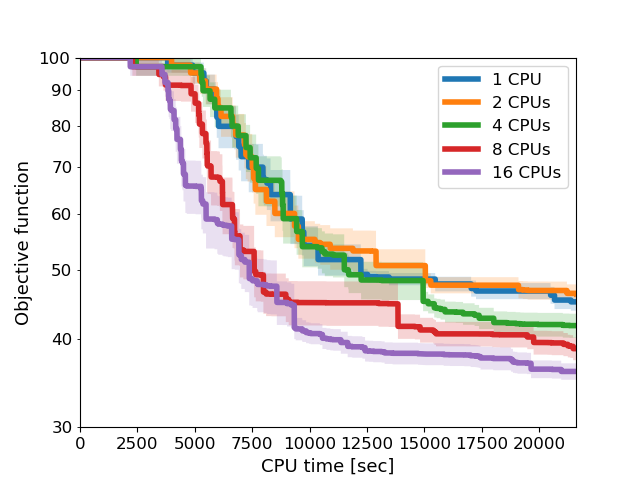
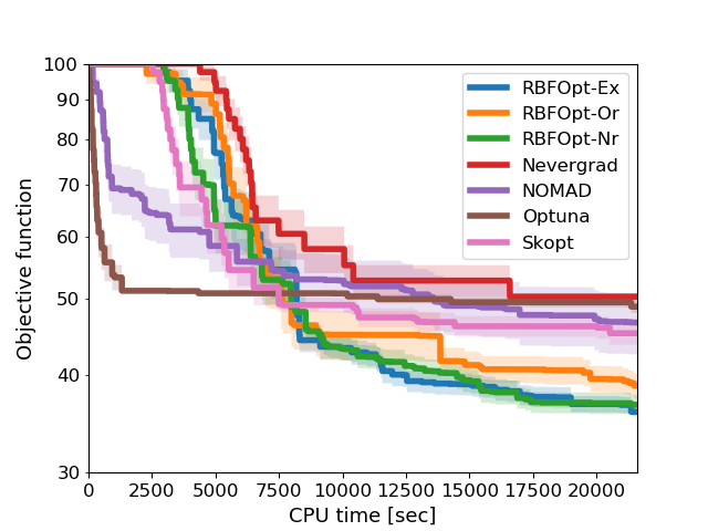
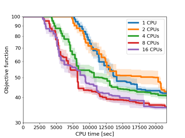

We evaluate the performance of the optimization algorithm to optimize the hyperparameters of a random forest classifier on a specific dataset. We use the RandomForestClassifier class implemented in Scikit-learn [28], trained on the “forest cover type” dataset. This is a classification dataset with 581012 samples of dimension 54, and 7 classes; see http://archive.ics.uci.edu/ml/datasets/Covertype for more information. The RandomForestClassifier has 10 hyperparameters, listed in Table 5; three of them are categorical, but one of them has only two possible values (the “criterion” parameter) and it is therefore treated as a binary variable. We evaluate the performance of a classifier by 5-fold cross validation, and use the average performance on the test set as the objective function. To transform it into a minimization problem, we computed the objective function as minus the recorded accuracy. The CPU time for a single evaluation of the objective function varies a lot, depending on the chosen hyperparameters; it is typically between and seconds, but it can take up to a few hours. We use default values for all parameters of RBFOpt. We compare several algorithms:
- •
RBFOpt with the extended space formulation of categorical variables;
- •
RBFOpt with the original space formulation of categorical variables;
- •
Nevergrad with the TwoPointsDE algorithm, which has the best performance for small in the experiments of Sect. 5.4;
- •
NOMAD, using the p-MADS parallel version;
- •
Optuna;
- •
Scikit-Optimize, using the gp base estimator and one-hot encoding for categorical variables.
SMAC is excluded from this set of experiments due to technical problems when running the available beta version on multiple CPUs. We additionally tested the Coop-MADS variant of NOMAD, but we do not report the corresponding results because p-MADS proved to be superior on this problem instance. Note that the one-hot encoding employed in Scikit-Optimize uses the same principle as the extended space formulation of this paper. The wall-clock time limit is set to 6 hours for all algorithms.
We run 20 different random seeds for each of these algorithms, using these seeds to initialize the optimization algorithms and the training of the classifier, thereby making the training deterministic and reproducible. As remarked in Sect. 5.4, RBFOpt and NOMAD assume that the objective function is deterministic, therefore fixing the random seeds is justified for these algorithms. For the remaining solvers, which target hyperparameter optimization problems, the random seed does not have to be fixed and in principle their performance could improve if we allow the solvers to evaluate the same point multiple times with different random seeds for the training phase. In particular, with our setup each algorithm observes only one realization of the chosen generalization error estimator (i.e., accuracy using 5-fold cross validation) for a given values of the hyperparameters, whereas hyperparameter optimization solvers can in principle observe multiple realizations and use this information to their advantage. We do not explore this possibility, noting that given the relatively tight wall-clock time limit, we expect the approach described above (i.e., fixed random seed for each run) to be a reasonable trade off. We report the average objective function value over time, where the average is taken with respect to the 20 random seeds. Results are given in Fig. 7. The runs corresponding to the same random seed are initialized with the same set of points for RBFOpt, Nevergrad and Scikit-Optimize: this has the goal of reducing variance in the experiments. NOMAD is initialized using the first point in the latin hypercube design generated by RBFOpt, while Optuna uses its own initialization strategy.
In Fig. 7(a) and 7(c) we plot the objective function value for RBFOpt in original and extended space, respectively, using up to 16 CPUs. The plots showcase the benefits of asynchronous parallel optimization when the main concern is the wall-clock time, rather than overall efficiency of the search in terms of the number of objective function evaluations. When using multiple CPUs, not only we improve the objective function much faster, but we eventually find better solutions on average. Furthermore, the extended space formulation performs noticeably better than the original space formulation, supporting our conclusions from Sect. 5.3.
In Fig. 7(b) we compare several variants of RBFOpt with other solvers, using 8 CPUs. We choose 8 CPUs rather than 16 so that the problem is still moderately difficult. The plots indicate that RBFOpt, in all its variants, attains lower objective function values than all the remaining solvers, and the corresponding curves are below the other solvers for most of the time interval considered. The plots for NOMAD and Optuna decrease much faster than the other algorithms at the very beginning, but this is mostly due to the fact that both NOMAD and Optuna report the result of each function evaluation immediately, whereas the other algorithms only report results after evaluating a first batch of 16 points using Python’s multiprocessing.Pool. This implies that for NOMAD and Optuna the curves start improving after the first evaluation, whereas for all other algorithms no improvement is reported until the first 16 function evaluations are completed. To put all algorithms on equal footing, we plot the same data in Fig. 7(d), with the difference that we now assign to the first 15 function evaluations the same time stamp as the 16th. In this fairer setting, NOMAD and Optuna no longer enjoy an advantage in the early stages of the optimization. We point out that in the recent paper [19], NOMAD is shown to be more effective than RBFOpt on problems with heavily constrained feasible regions: on those problems, the local nature of NOMAD allows staying inside the (black-box) constraints, while the global nature of RBFOpt leads to the exploration of a large proprtion of infeasible points, even if their violation is penalized. However, the problem considered in this section is unconstrained, and RBFOpt improves the objective function more quickly than NOMAD or any of the other solvers.
Summarizing, RBFOpt performs better than all other tested algorithms on this hyperparameter optimization problem; among RBFOpt variants, compared using 8 CPUs, the extended space formulation has a clear advantage, and the Refinement step has little impact in these experiments, even though it was highly beneficial in our previous tests.
6 Conclusion
Our extensive numerical evaluation indicates that many ingredients contribute to the effectiveness of the optimization algorithm implemented in RBFOpt. More precisely, this paper explores the impact of different ways of modeling categorical variables (and discusses how to deal with the ensuing difficulties), the use of RBF interpolants without the unisolvence property, refinement search to locally improve solutions, and asynchronous parallel optimization. Individually, each of these components provides some benefit, with the refinement search having the most noticeable impact in serial optimization. Together, they contribute to a powerful optimization algorithm that appears to be one of the most efficient derivative-free solvers available for highly nonconvex problems, and that is capable of handling unconstrained mixed-variable problems.
References
- [1] Takuya Akiba, Shotaro Sano, Toshihiko Yanase, Takeru Ohta, and Masanori Koyama. Optuna: A next-generation hyperparameter optimization framework. In Proceedings of the 25rd ACM SIGKDD International Conference on Knowledge Discovery and Data Mining, 2019.
- [2] Charles Audet and J.E. Dennis Jr. Mesh adaptive direct search algorithms for constrained optimization. SIAM Journal on Optimization, 17(1):188–217, 2004.
- [3] Charles Audet and John E Dennis Jr. Pattern search algorithms for mixed variable programming. SIAM Journal on Optimization, 11(3):573–594, 2001.
- [4] Charles Audet, Michael Kokkolaras, Sébastien Le Digabel, and Bastien Talgorn. Order-based error for managing ensembles of surrogates in mesh adaptive direct search. Journal of Global Optimization, 70(3):645–675, 2018.
- [5] P. Bonami, L.T. Biegler, A.R. Conn, G. Cornuéjols, I.E. Grossmann, C.D. Laird, J. Lee, A. Lodi, F. Margot, N. Sawaya, and A. Wächter. An algorithmic framework for convex Mixed Integer Nonlinear Programs. Discrete Optimization, 5(2):186–204, 2008.
- [6] Andrew R Conn, Nicholas IM Gould, and Philippe L Toint. Trust region methods. SIAM, 2000.
- [7] Andrew R Conn, Katya Scheinberg, and Luís N Vicente. Geometry of interpolation sets in derivative free optimization. Mathematical programming, 111(1-2):141–172, 2008.
- [8] Andrew R Conn, Katya Scheinberg, and Luís N Vicente. Global convergence of general derivative-free trust-region algorithms to first-and second-order critical points. SIAM Journal on Optimization, 20(1):387–415, 2009.
- [9] Alberto Costa, Emanuele Di Buccio, Massimo Melucci, and Giacomo Nannicini. Efficient parameter estimation for information retrieval using black-box optimization. IEEE Transactions on Knowledge and Data Engineering, 30(7):1240–1253, 2018.
- [10] Alberto Costa and Giacomo Nannicini. RBFOpt: an open-source library for black-box optimization with costly function evaluations. Mathematical Programming Computation, 10(4):597–629, 2018. doi:10.1007/s12532-018-0144-7.
- [11] Gonzalo I. Diaz, Achille Fokoue, Giacomo Nannicini, and Horst Samulowitz. An effective algorithm for hyperparameter optimization of neural networks. IBM Journal of Research and Development, 61(4/5), 2017.
- [12] L.C.W. Dixon and G.P. Szego. The global optimization problem: an introduction. In L.C.W. Dixon and G.P. Szego, editors, Towards Global Optimization, pages 1–15. North Holland, Amsterdam, 1975.
- [13] Wilna Du Toit. Radial basis function interpolation. PhD thesis, Stellenbosch: Stellenbosch University, 2008.
- [14] David Eriksson, David Bindel, and Christine Shoemaker. Surrogate optimization toolbox (pysot), 2015. URL: http://github.com/dme65/pySOT.
- [15] David Eriksson, Michael Pearce, Jacob Gardner, Ryan D Turner, and Matthias Poloczek. Scalable global optimization via local Bayesian optimization. In Advances in Neural Information Processing Systems, pages 5496–5507, 2019.
- [16] Hans-Martin Gutmann. A radial basis function method for global optimization. Journal of Global Optimization, 19(3):201–227, 2001. doi:10.1023/A:1011255519438.
- [17] Tim Head, MechCoder, Gilles Louppe, Iaroslav Shcherbatyi, fcharras, Zé Vinícius, cmmalone, Christopher Schröder, nel215, Nuno Campos, Todd Young, Stefano Cereda, Thomas Fan, rene rex, Kejia (KJ) Shi, Justus Schwabedal, carlosdanielcsantos, Hvass-Labs, Mikhail Pak, SoManyUsernamesTaken, Fred Callaway, Loïc Estève, Lilian Besson, Mehdi Cherti, Karlson Pfannschmidt, Fabian Linzberger, Christophe Cauet, Anna Gut, Andreas Mueller, and Alexander Fabisch. scikit-optimize/scikit-optimize: v0.5.2, March 2018. doi:10.5281/zenodo.1207017.
- [18] Frank Hutter, Holger H Hoos, and Kevin Leyton-Brown. Sequential model-based optimization for general algorithm configuration. In International Conference on Learning and Intelligent Optimization, pages 507–523. Springer, 2011.
- [19] Dounia Lakhmiri, Sébastien Le Digabel, and Christophe Tribes. Hypernomad: Hyperparameter optimization of deep neural networks using mesh adaptive direct search. arXiv preprint arXiv:1907.01698, 2019.
- [20] S. Le Digabel. Algorithm 909: NOMAD: Nonlinear optimization with the mads algorithm. ACM Transactions on Mathematical Software, 37(4):44:1–44:15, 2011. URL: http://dx.doi.org/10.1145/1916461.1916468, doi:10.1145/1916461.1916468.
- [21] Giampaolo Liuzzi, Stefano Lucidi, and Francesco Rinaldi. An algorithmic framework based on primitive directions and nonmonotone line searches for black-box optimization problems with integer variables. Mathematical Programming Computation, 12(4):673–702, 2020.
- [22] MINLP Library 2. URL: http://www.gamsworld.org/minlp/minlplib2/html/.
- [23] Jorge Moré and Stefan M. Wild. Benchmarking derivative-free optimization algorithms. SIAM Journal on Optimization, 20(1):172–191, 2009.
- [24] Juliane Müller. MISO: mixed-integer surrogate optimization framework. Optimization and Engineering, pages 1–27, 2015. Online first. URL: http://dx.doi.org/10.1007/s11081-015-9281-2, doi:10.1007/s11081-015-9281-2.
- [25] Juliane Müller, Christine A. Shoemaker, and Robert Piché. SO-MI: A surrogate model algorithm for computationally expensive nonlinear mixed-integer black-box global optimization problems. Computers & Operations Research, 40(5):1383–1400, 2013. URL: http://www.sciencedirect.com/science/article/pii/S0305054812001967, doi:http://dx.doi.org/10.1016/j.cor.2012.08.022.
- [26] Arnold Neumaier. Neumaier’s collection of test problems for global optimization. Retrieved in May 2014. URL: http://www.mat.univie.ac.at/~neum/glopt/my_problems.html.
- [27] C.H. Papadimitriou and K. Steiglitz. Combinatorial Optimization: Algorithms and Complexity. Dover, New York, 1998.
- [28] F. Pedregosa, G. Varoquaux, A. Gramfort, V. Michel, B. Thirion, O. Grisel, M. Blondel, P. Prettenhofer, R. Weiss, V. Dubourg, J. Vanderplas, A. Passos, D. Cournapeau, M. Brucher, M. Perrot, and E. Duchesnay. Scikit-learn: Machine learning in Python. Journal of Machine Learning Research, 12:2825–2830, 2011.
- [29] Mike JD Powell. Five lectures on radial basis functions. Informatics and Mathematical Modelling, Technical University of Denmark, DTU, 2005.
- [30] J. Rapin and O. Teytaud. Nevergrad - A gradient-free optimization platform. https://GitHub.com/FacebookResearch/Nevergrad, 2018.
- [31] Rommel G Regis. An initialization strategy for high-dimensional surrogate-based expensive black-box optimization. In Modeling and Optimization: Theory and Applications, pages 51–85. Springer, 2013.
- [32] Rommel G Regis. Constrained optimization by radial basis function interpolation for high-dimensional expensive black-box problems with infeasible initial points. Engineering Optimization, 46(2):218–243, 2014.
- [33] Rommel G. Regis and Christine A. Shoemaker. A stochastic radial basis function method for the global optimization of expensive functions. INFORMS Journal on Computing, 19(4):497–509, 2007. doi:10.1287/ijoc.1060.0182.
- [34] Giorgio Sartor. Large-scale Constrained Black-box Optimization: Theory, Methodology, and Applications. PhD thesis, Singapore University of Technology and Design, 2017.
- [35] James David Schaffer. Some experiments in machine learning using vector evaluated genetic algorithms. PhD thesis, Vanderbilt University, 1984.
- [36] Fabio Schoen. A wide class of test functions for global optimization. Journal of Global Optimization, 3(2):133–137, 1993.
- [37] Jasper Snoek, Hugo Larochelle, and Ryan P Adams. Practical bayesian optimization of machine learning algorithms. Advances in neural information processing systems, 25:2951–2959, 2012.
- [38] A. Wächter and L. T. Biegler. On the implementation of a primal-dual interior point filter line search algorithm for large-scale nonlinear programming. Mathematical Programming, 106(1):25–57, 2006.
- [39] Stefan M. Wild and Christine Shoemaker. Global convergence of radial basis function trust-region algorithms for derivative-free optimization. SIAM Review, 55(2):349–371, 2013.