Email: {ydyangdu@163.com, zhangshunsdu@xidian.edu.cn,
feifeigao@ieee.org, cxu@nwafu.edu.cn, jpmaxdu@gmail.com, odobre@mun.ca}
Deep Learning Based Antenna Selection for Channel Extrapolation in FDD Massive MIMO
Abstract
In massive multiple-input multiple-output (MIMO) systems, the large number of antennas would bring a great challenge for the acquisition of the accurate channel state information, especially in the frequency division duplex mode. To overcome the bottleneck of the limited number of radio links in hybrid beamforming, we utilize the neural networks (NNs) to capture the inherent connection between the uplink and downlink channel data sets and extrapolate the downlink channels from a subset of the uplink channel state information. We study the antenna subset selection problem in order to achieve the best channel extrapolation and decrease the data size of NNs. The probabilistic sampling theory is utilized to approximate the discrete antenna selection as a continuous and differentiable function, which makes the back propagation of the deep learning feasible. Then, we design the proper off-line training strategy to optimize both the antenna selection pattern and the extrapolation NNs. Finally, numerical results are presented to verify the effectiveness of our proposed massive MIMO channel extrapolation algorithm.
I Introduction
With the increasing demand for the information transmission rate, massive multiple-input multiple-output (MIMO) system has become a key technology for the next generation of wireless communication [1]. The huge number of antennas in massive MIMO brings a great challenge for the base station (BS) to obtain the accurate channel state information (CSI), especially in frequency division duplex (FDD) mode[2]. In fact, it is possible to utilize microwave scattering reciprocity between uplink and downlink to reduce the overhead of the channel acquisition. In [3], the authors utilized the reciprocity property and proposed a closed-loop channel estimation scheme for the hybrid massive MIMO. Yu et al. [4] designed an efficient downlink channel reconstruction scheme for the FDD massive MIMO system. In [5], Li et al. utilized the expectation-maximization and optimal Bayesian Kalman filter methods to accurately track the downlink channel with partial prior knowledge achieved from the uplink training.
Since deep learning (DL) can effectively dig out the latent and complex relation among different data sets, researchers have attempted to utilize DL for improving the performance of the massive MIMO channel estimation. In [6], Wen et al. constructed a DL-based scheme to realize the downlink CSI sensing and to enhance the quality of CSI reconstruction at BS. Alkhateeb et al. in [7] utilized deep neural networks (DNNs) to approximate the complex mapping function among the channels related with different frequency bands and locations. Yang et al. in [8] proposed a DL-based uplink-to-downlink mapping scheme to infer downlink massive MIMO channels from the uplink ones. Choi et al. [9] developed a DL extrapolation technique to implement the CSI mapping between the downlink and the uplink, where the uplink channel path gains of low dimension were treated as the input of the neural networks (NNs).
As mentioned above, the uplink-to-downlink channel extrapolation has been widely examined within the massive MIMO framework. However, at millimeter wave band, the hybrid beamforming structure is usually adopted to decrease the hardware cost. Moreover, with the development of the extremely large massive MIMO, the hybrid mode may be the feasible way to enjoy the high spatial resolution. Under this structure, all the uplink CSI of all antenna elements cannot be acquired at the same time [10]. Even though we can scan all the antenna elements to achieve all CSI, it would spend the time resources. Intuitively, we can utilize the partial uplink CSI observed at a few antennas to extrapolate the full downlink one with the power of NNs.
Obviously, the performance of the downlink channel extrapolation from the partial uplink CSI is closely related with the antenna selection pattern. If the channels at different antenna elements are independent, the uniform selection pattern would be the best choice. However, in massive MIMO system, the distance between antenna elements can be small enough that there exists strong correlation among the channels. Under this scenario, the uniform selection pattern may not be the optimal scheme. So, how to select the antenna subset for uplink channel estimation is very important. In the model-based MIMO signal processing frameworks, there are many effective methods to complete the antenna selection through solving the discrete combinatorial optimization [11, 12, 13]. However, the DL-based channel extrapolation mainly lies in the huge data learning without of the accurate model and cannot directly incorporate the traditional antenna selection schemes [6]–[9]. Thus, we should design proper DL-based antenna selection and effectively extrapolate the downlink channels from the partial uplink ones. In this paper, we resort to the probabilistic sampling theory and model the discrete antenna selection as a continuous and differentiable function. In such way, we can design the proper off-line DL training strategy to optimize both the antenna selection pattern and the extrapolation NNs through efficient back propagation.

II Channel Model
We consider a massive MIMO system, which contains one BS and one user. The BS is equipped with antennas in the form of non-uniform linear array (NULA)11 1 Theoretically, compared with uniform linear array (ULA), the NULA can obtain a narrower beam without increasing the number of array elements [14]. The irregular physical structure would aggregate the non-uniform distribution of the massive MIMO channel. [14], and the user is equipped with single antenna. The coordinate vector of the antenna position is . Let denote the channel from the user to the BS at frequency . Assume that the channel between the user and the BS consists of paths. Therefore, the channel vector can be written as [15]
| (1) |
where , with as the transpose operator. The -th path has a delay , a phase shift and a propagation gain . Moreover, the spatial steering vector at BS is defined as
| (2) |
where is the speed of light and denotes the direction of arrival of the -th path.
III DL-based Antenna Selection
In FDD, there is a frequency offset between the uplink and downlink channels. Let us denote and as uplink and downlink channels at frequencies and , respectively. Due to the limited number of radio channels in the hybrid beamforming structure, we assume that not all the elements in can be achieved, which means that massive MIMO channels are spatially sub-sampled. In other words, we should determine which antennas should be selected to extrapolate the downlink channels. As shown in Fig. 1, our goal is to utilize these sub-sampled data to extrapolate the full elements in , where DNN will be utilized. In this section, we will successively introduce the framework design, loss function and learning strategy for the antenna selection based massive MIMO channel extrapolation.
III-A Framework Design
As mentioned above, we need to solve the following mapping relationships:
| (3) |
where represents the uplink channel after sub-sampling.

As shown in Fig. 2, our framework contains two parts, i.e., the antenna selection and the channel extrapolation. The former sub-samples the original uplink vector to achieve the vector as
| (4) |
where and represents the antenna selection operation. We can define the spatial compression ratio of the massive MIMO channel as . Correspondingly, within the latter part, we resort to the DNN to reconstruct the downlink channels from as
| (5) |
where the vector represents the recovery version of , and the function is the extrapolation operation by DNN.
Our aim is to effectively achieve the antenna selection pattern and the extrapolation scheme with DL, where the back propagation is usually involved. However, the antenna selection operation is a discrete combination operation, which hinders the implementation of the back propagation. To overcome this bottleneck, we introduce the probabilistic sampling strategy as follows.
III-B Learning the Antenna Selection Pattern
The antenna selection function can be expressed by the binary sub-sampling matrix 22 2 Here, our aim is to decrease the active antennas at the same time. Theoretically, different antenna selection patterns can be adopted from time to time. However, frequently antenna switching may take some signaling overhead for the system and decrease its energy efficiency. Accordingly, we consider that the antenna selection operation is stable within a long interval. , where the elements of are either 0 or 1, and the vector contains only one non-zero element. Then, we have
| (6) |
Within the probabilistic sampling framework, can be defined as [16]
| (7) |
where is a categorical distributed random variable with the class probabilities . Notice that the result of is one real unit-vector and has only one non-zero entry, whose index corresponds to the class of the drawn sample. A larger means that the -th element of would be achieved from the -th antenna with higher probability. Different categorical variables, i.e., and , are independent, . Furthermore, we can reparameterize with the unnormalized log-probabilities as
| (8) |
Here we define the vectors and for further use. In order to achieve one effective sample from the categorical distribution, we resort to the - trick and generate a realization of as [17]
| (9) |
where , , …, are independent and identically distributed (i.i.d.) samples drawn from the distribution. Correspondingly, can be achieved from as
| (10) |
However, when we do the above operation from to , the same antenna may be repeatly selected. To avoid this case, we would dynamically exclude the categories (antennas), that have already been chosen, renormalize the log-probabilities of the rest categories, and then implement the - trick. Before proceeding, we define .
Within DL framework, we should iteratively update through the back propagation to complete the antenna selection. However, the operator is is not differentiable. Thus, we will resort to the function as a continuous and differentiable approximation of . Then, we have [16]
| (11) |
where the temperature controls the softness of . The lower is, the closer the generated Gumbel-Softmax distribution is to the categorical distribution. During training, we will gradually reduce the temperature to approach the true discrete distribution. Then, the first-order derivative of with respect to can be written as
| (12) |
III-C DNN-based Channel Extrapolation
The channel extrapolation is implemented within DNN . Firstly, we reshape the raw input data of DNN, i.e., , as
| (13) |
and input into DNN. Correspondingly, the output of DNN is . The DNN adopts the fully-connected (FC) NN architecture with layers, The output is a cascade of the nonlinear transformation with respect to , i.e.,
| (14) |
where is the trainable parameter vector of DNN. Then, each layer computation of the DNN can be expressed as
| (15) |
where is the weight vector associated with the and layers, while and are the bias vector and the activation function of the layer, respectively.
Finally, we can obtain the extrapolated massive MIMO downlink channel vector from the real data .
III-D Learning Scheme
Before proceeding, let us define and . During the network learning stage, we train the model parameters and by minimizing the mean squared error (MSE) between the output and the target . Without loss of generality, we use the MSE of the channel estimation as the loss function, which can be written as
| (16) |
where is the -norm of vector , and is the batch size. Besides, we promote training towards one-hot distributions through penalizing convergence towards high entropy distribution as
| (17) |
When the sub-sampling and extrapolation parameters are updated jointly, the resultant optimization problem can be written as:
| (18) |
where the penalty multiplier evaluates the importance of the different penalties. Here, the adaptive moment estimation (Adam) [18] optimizer algorithm is adopted to achieve the optimal model parameters and . Moreover, we use different -learning rate and -learning rate update for and respectively, where .
As mentioned above, the temperature parameter should be gradually decreased to achieve the discrete distribution. Thus, we set the initialization of as 5.0 and gradually reduce it to 0.5 during training. To promote preservation of the original order, all elements are initialized as
| (19) |
where , , and .
For clarity, we present the detailed learning steps for both antenna selection and channel extrapolation in Algorithm 1.
IV Simulation Results
In this section, we numerically evaluate the performance of our proposed DL and antenna selection based massive MIMO channel extrapolation method. We first describe the communication scenario and dataset source, and then introduce the NN parameters. Finally, the performance evaluation of the simulation results is explained. Moreover, the performance of the DL and uniform antenna selection based channel extrapolation is also examined for comparison.
We consider the indoor distributed massive MIMO scenario ‘I1’ of the DeepMIMO dataset [15], which is generated based on the Wireless InSite software. Correspondingly, the primary parameters for this case are listed in TABLE I. For the spacing setting of NULA, we repeat the vector of the 16 antennas four times to achieve the spacing vector for the 64 antennas [19], where represents the carrier wavelength along the uplink. With respect to ULA, the antenna spacing is set as . Furthermore, within the DeepMIMO dataset, we activate the users located within the region formed by the 1-st row to the 512-th row. Then, the number of active users from 1 to 512 is 90862. The bandwidth of orthogonal frequency division multiplexing (OFDM) is set as 20 MHz, while the number of sub-carriers is 64. The generated channel samples with the above parameters are divided into training and testing sets according to the ratio of . These data sets are used for the DNN learning and performance evaluation.
| Parameter | Value |
|---|---|
| Name of scenario | I1 |
| The carrier frequency of uplink and downlink | 2.4GHz, 2.5GHz |
| Number of BS antennas in (x, y, z) | (1, 1, 64) |
| Number of paths | 5 |
| Active users | Row 1 to 502 |
| System bandwidth | 20 MHz |
| Number of OFDM sub-carriers | 64 |
Each NN layer contains FC and activation function. In the hidden layers, the number of neurons is set as by trails and adjustments, and is adopted as the activation function, i.e., . With respect to the input and output layers, the numbers of the neurons are same with the sizes of the input and output data vectors, i.e., and , respectively. The initial parameters for the learning rate are and , the penalty multiplier is taken as , and the batch size is 32.
Fig. 3 depicts the channel extrapolation MSE of the proposed method versus the spatial compression ratio . In the figure, the curves labeled by ‘uniform’ correspond to the DL and uniform antenna selection based method, while the ones marked by ‘proposed method’ represent the performance of our proposed method. It can be checked that our method can always achieve better extrapolation performance than the uniform antenna selection based scheme for both ULA and NULA. Specially, compared to the case with ULA, our scheme can achieve higher performance gain under the NULA scenario, which is because that the channels from NULA possess much more non-uniform data structure than that from ULA. On the other hand, all the MSE curves decrease when increases from 1/16 to 1/2.
Table II and Table III present the sequence number of the selected antennas under different in NULA and ULA, respectively.

| The sampled antennas | |
|---|---|
| 1/2 | 1, 5, 6, 7, 9, 10, 13, 14, 16, 17, 20, 22, 25, 26, 29, 31, 33, |
| 34, 37, 38, 41, 43, 44, 46, 47, 48, 53, 56, 58, 59, 60, 63 | |
| 1/4 | 5, 7, 14, 18, 20, 23, 26, 31, 34, 38, 43, 46, 50, 56, 59, 62 |
| 1/8 | 6, 14, 23, 31, 38, 46, 54, 62 |
| 1/16 | 14, 30, 46, 62 |
| The sampled antennas | |
|---|---|
| 1/2 | 2, 4, 5, 7, 12, 13, 15, 17, 19, 21, 23, 25, 27, 29, 32, 33, 35, |
| 37, 39, 40, 42, 43, 45, 46, 48, 51, 53, 55, 57, 59, 61, 63 | |
| 1/4 | 3, 7, 11, 16, 19, 23, 27, 30, 35, 39, 43, 47, 51, 55, 59, 62 |
| 1/8 | 7, 14, 23, 31, 39, 47, 55, 61 |
| 1/16 | 15, 32, 47, 62 |
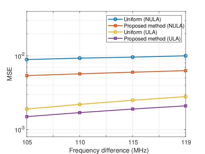
Fig. 4 presents the channel extrapolation capability of our method with different frequency gaps between and , where . We consider 4 different frequency gaps for both ULA and NULA. is generated from the first subcarrier at 2.4 GHz band, while are separately sampled at the 17-th, 33-th, 49-th and 62-th sub-carriers along the 2.5 GHz downlink. Obviously, as the frequency difference increases, the MSE increases, however the performance impact is not very large, which means that the antenna selection method and the NN can achieve good channel extrapolation with big frequency gap.

In practice, there exist channel estimation errors along the uplink, which may bring some impacts on our proposed scheme. Without loss of generality, we model the uplink channel estimation as , where denotes the additive white Gaussian noise vector. Then, the variance of represents the uplink channel estimation MSE. Correspondingly, we aim to recover with . In Fig. 5, we evaluate the MSEs of downlink channel extrapolation when the uplink channel estimation has different MSE values, when ULA is applied. As can be seen from Fig. 5, with the decreasing of the uplink channel estimation MSEs, the extrapolation performance of the downlink massive MIMO channels improves within both uniform antenna selection based and our proposed schemes. The uplink channel estimation errors do not affect the performance gain of our scheme over the uniform antenna selection based one. The two schemes can effectively de-noise the uplink estimated channels under ’s high MSE region. The above observation is reasonable and can be explained as follows. The performance of DL based extrapolation scheme is determined by both the initial input and the performance gain of the NN. Moreover, compared with uniform antenna selection based framework, our scheme utilizes DL to learn better selection pattern.
V Conclusion
In this paper, we examined DL and antenna selection based massive MIMO channel extrapolation scheme. First, we introduced the probabilistic sampling method to implement the antenna selection. Then, we inputed the sub-sampled uplink massive MIMO channels into a DNN, and extrapolated the full downlink massive MIMO channels with partial uplink CSI. The Simulation results showed that our proposed scheme could achieve better performance than the DL and uniform antenna selection based one and could work effectively with big frequency gaps and uplink channel estimation errors.
References
- [1] F. Rusek, D. Persson, B. K. Lau, E. G. Larsson, T. L. Marzetta, O. Edfors, and F. Tufvesson, “Scaling up MIMO: Opportunities and challenges with very large arrays,” IEEE Signal Process. Mag., vol. 30, no. 1, pp. 40–60, Jan. 2013.
- [2] S. Noh, M. D. Zoltowski, and D. J. Love, “Training sequence design for feedback assisted hybrid beamforming in massive MIMO systems,” IEEE Trans. Commun., vol. 64, no. 1, pp. 187–200, Jan. 2016.
- [3] A. Liao, Z. Gao, H. Wang, S. Chen, M. Alouini and H. Yin, “Closed-loop sparse channel estimation for wideband millimeter-wave full-dimensional MIMO systems,” IEEE Trans. Commun., vol. 67, no. 12, pp. 8329-8345, Dec. 2019.
- [4] Y. Han, T. Hsu, C. Wen, K. Wong and S. Jin, “Efficient downlink channel reconstruction for FDD multi-antenna systems,” IEEE Trans. Wireless. Commun., vol. 18, no. 6, pp. 3161–3176, Jun. 2019.
- [5] M. Li, S. Zhang, N. Zhao, W. Zhang, and X. Wang, “Time-varying massive MIMO channel estimation: Capturing, reconstruction and restoration,” IEEE Trans. Commun., vol. 67, no. 11, pp. 7558–7572, Nov. 2019.
- [6] C. Wen, W. Shih, and S. Jin, “Deep learning for massive MIMO CSI feedback,” IEEE Wireless Commun. Lett., vol. 7, no. 5, pp. 748–751, Oct. 2018.
- [7] M. Alrabeiah and A. Alkhateeb, “Deep learning for TDD and FDD massive MIMO: Mapping channels in space and frequency,” in Proc. 53rd Asilomar Conference on Signals, Systems, and Computers, Pacific Grove, CA, USA, Nov. 2019, pp. 1465-1470.
- [8] Y. Yang, F. Gao, G. Y. Li, and M. Jian, “Deep learning-based downlink channel prediction for FDD massive MIMO system,” IEEE Commun. Lett., vol. 23, no. 11, pp. 1994–1998, Nov. 2019.
- [9] H. Choi and J. Choi, “Downlink extrapolation for FDD multiple antenna systems through neural network using extracted uplink path gains,” IEEE Access, vol. 8, pp. 67100–67111, Apr. 2020.
- [10] O. E. Ayach, S. Rajagopal, S. Abu-Surra, Z. Pi, and R. W. Heath, “Spatially sparse precoding in millimeter wave MIMO systems,” IEEE Trans. Wireless. Commun., vol. 13, no. 3, pp. 1499–1513, Mar. 2014.
- [11] Y. Gao, H. Vinck, and T. Kaiser, “Massive MIMO antenna selection: Switching architectures, capacity bounds, and optimal antenna selection algorithms,” IEEE Trans. Signal Process., vol. 66, no. 5, pp. 1346–1360, Mar. 2018.
- [12] S. Asaad, A. M. Rabiei, and R. R. Müller, “Massive MIMO with antenna selection: Fundamental limits and applications,” IEEE Trans. Wireless Commun., vol. 17, no. 12, pp. 8502–8516, Dec. 2018.
- [13] P. V. Amadori, and C. Masouros, “Interference-driven antenna selection for massive multiuser MIMO,” IEEE Trans. Veh. Technol., vol. 65, no. 8, pp. 5944–5958, Aug. 2016.
- [14] W. Liu and Z. Wang, “Non-uniform full-dimension MIMO: New topologies and opportunities,” IEEE Wireless. Commun., vol. 26, no. 2, pp. 124-132, Apr. 2019.
- [15] A. Alkhateeb, “DeepMIMO: A generic deep learning dataset for millimeter wave and massive MIMO applications,” in Proc. Information Theory and Applications Workshop (ITA), San Diego, CA, Feb. 2019, pp. 1–8.
- [16] Iris A.M. Huijben, Bastiaan S. Veeling and Ruud J.G. van Sloun, “Deep probabilistic subsampling for task-adaptive compressed sensing,” in Proc. International Conference on Learning Representations, Addis Ababa, Ethiopia, Apr. 2020.
- [17] E. Gumbel. Statistical theory of extreme values and some practical applications. NBS Applied Mathematics Series, 33, 1954.
- [18] D. P. Kingma and J. Ba, “ADAM: A method for stochastic optimization,” arXiv:1412.6980, 2014, [Online]. Available: https://arxiv.org/abs/1412.6980
- [19] L. Wei, W. Shao, W. Qi, and J. Chen, “Peak-to-peak search: fast and accurate DOA estimation method for arbitrary non-uniform linear array”. Electron. Lett., vol. 51, no. 25, pp. 2078-2080, Dec. 2015.