Unfolding-Model-Based Visualization: Theory, Method and Applications

Consider $N$ respondents making choice on $J$ binary items (e.g., “agree/disagree”). Let $Y_{ij}$ be a random variable, denoting the response from respondent $i$ to item $j$, taking value 0 or 1, and let $y_{ij}$ be its realization. For example, such data can come from senate roll call voting, where the respondents are senators and the items correspond to roll calls. Response $Y_{ij}=1$ means that senator $i$ supports roll call $j$ and $Y_{ij}=0$ otherwise.

We provide a simulated example in Figure 1 to illustrate MDU analysis. Panel (a) shows the heat map of an observed response matrix which consists of 20 respondents and 10 items, where 0 and 1 responses are represented by red and green colors, respectively. Given choice data in panel (a), an MDU method aims at representing respondents and items by ideal points in the same low-dimensional Euclidian space $\mathbb{R}^{K}$ as in panel (b) of Figure 1 that can be easily visualized, where the respondent-respondent, respondent-item, and item-item relationships are captured by the between-points distance. The dimension $K$ of the Euclidian space is often set to be 2 or 3 for the purpose of visualization.

One way to conduct MDU is via a statistical model. An MDU model typically assumes that each respondent/item is associated with a true ideal point in $\mathbb{R}^{K}$ that is represented by a $K$-dimensional parameter vector. Let $\boldsymbol{\theta}_{i}=(\theta_{i1},...,\theta_{iK})^{\top}$ and $\mbox{$\mathbf{a}$}_{j}=(a_{j1},...,a_{jK})^{\top}$ denote the parameter vectors of respondent $i$ and item $j$, respectively. It is assumed that response $Y_{ij}$ is determined by the Euclidian distance between $\boldsymbol{\theta}_{i}$ and $\mbox{$\mathbf{a}$}_{j}$ in $\mathbb{R}^{K}$. Finally, we use $\Theta^{N}=(\theta_{ik})_{N\times K}$ and $A^{J}=(a_{jk})_{J\times K}$ to denote the matrices containing all the person and the item ideal points, respectively. Under such a statistical model, the goal of MDU becomes to estimate the person and item parameters based on data.

In this paper, we focus on MDU models taking the form

where $\|\cdot\|$ denotes the standard $L_{2}$ norm and $f:[0,\infty)\rightarrow[0,1]$ is a pre-specified link function. It is assumed that the responses $Y_{ij}$ are conditionally independent, given the ideal points $\boldsymbol{\theta}_{i}$ and $\mbox{$\mathbf{a}$}_{j}$, $i=1,...,N,j=1,...,J$. This model falls under the general framework of the MDU threshold model for binary choice data (DeSarbo and Hoffman, 1987, see). According to the form of (1), the distribution of data only depends on the squared distance between every pair of person and item ideal points, $d_{ij}=\|\boldsymbol{\theta}_{i}-\mbox{$\mathbf{a}$}_{j}\|^{2},i=1,...,N,j=1,...,J$. The matrix $D_{N,J}=(d_{ij})_{N\times J}$ is known as the corresponding partial distance matrix, where the subscripts of $D_{N,J}$ emphasize the dependence of this matrix on the numbers of respondents and items.

In addition, the link function $f$ is often assumed to be a monotone decreasing function, so that a larger distance implies a lower probability of $Y_{ij}=1$. An example of such a link function is $f(x)={2}/{(1+\exp(x))}$. When $f(x)$ takes this form, $P(Y_{ij}=1\mid\boldsymbol{\theta}_{i},\mbox{$\mathbf{a}$}_{j})=1$ when the distance between $\boldsymbol{\theta}_{i}$ and $\mbox{$\mathbf{a}$}_{j}$ is 0, i.e., the two points are identical, and the probability $P(Y_{ij}=1\mid\boldsymbol{\theta}_{i},\mbox{$\mathbf{a}$}_{j})$ decays towards 0 when the distance increases.

In what follows, we provide two remarks on this modeling framework.

Our main goal is the simultaneous recovery of the ideal points $\boldsymbol{\theta}_{i}$ and $\mbox{$\mathbf{a}$}_{j}$, based on the observed binary responses $y_{ij},i=1,...,N,j=1,...,J$. Since the model only relies on the Euclidian distance between the ideal points, two sets of points lead to the same model if they have the same configuration, i.e., one set of points can be obtained by applying an isometry mapping to the other. This is because, the distance between points is invariant under an isometry mapping. An isometry mapping $F$ in $\mathbb{R}^{K}$ takes the form

where $O$ is a $K\times K$ orthogonal matrix and $\mathbf{b}$ is a vector in $\mathbb{R}^{K}$ (Olver, 1999, see, e.g.,). We further denote $\mathcal{A}_{K}$ as the set of all isometry mappings on $\mathbb{R}^{K}$. Without additional information, the best possible result one can expect is recovering the ideal points up to an isometry mapping. We refer to this problem as the recovery of ideal point configuration.

It is worth noting that regularity conditions are needed to ensure the recovery of the configuration. That is, it is possible that there exist multiple sets of ideal points with different configurations that lead to the same distribution of $Y_{ij}$s. In other words, the configuration of $\{\boldsymbol{\theta}_{1},...,\boldsymbol{\theta}_{N},\mbox{$\mathbf{a}$}_{1},...,\mbox{$\mathbf{a}$}_{J}\}$ may not be unique only given the partial distance matrix. This is known as the situation of degeneration, in which case the visualization does not convey information or can even be misleading. A simple example is given in Figure 2, where the two different configurations in the two panels have the same partial distance matrix.

Following the above discussion, the validity of unfolding-model-based visualization relies on the accuracy of configuration recovery, a problem to be discussed. Specifically, we consider the following loss function for configuration recovery,

where $\boldsymbol{\theta}_{i}^{*}$ and $\mbox{$\mathbf{a}$}_{j}^{*}$ denote the true ideal points and $\hat{\boldsymbol{\theta}}_{i}$ and $\hat{\mbox{$\mathbf{a}$}}_{j}$ denote the estimates from data $(y_{ij})_{N\times J}$. Note that (3) quantifies the accuracy of configuration recovery in an average sense, where isometry indeterminacy is bypassed by the minimization in (3) with respect to all isometry mappings in $\mathcal{A}_{K}$. We call (3) the average loss for the recovery of ideal point configuration. Error bounds will be established for (3) under reasonable conditions, which ensures the accurate recovery of the loss function when both $N$ and $J$ are large.

MDU is closely related to MDS, a class of methods for visualizing the similarity pattern between data points (Borg and Groenen, 2005). More precisely, MDS maps a set of variables onto a low dimensional space, based on data measuring the similarity between variables. As pointed out in Chapter 14, Borg and Groenen, 2005, MDU can be viewed as a special case of MDS, where the set of variables in MDS composes of both the respondents and items and the item response data $(y_{ij})_{N\times J}$ are regarded as measures of similarity between the respondents and the items, while the similarities within the two sets (i.e., respondents and items) are structurally missing; see Figure 3 for an illustration that is a reproduction of Figure 14.1 of Borg and Groenen, 2005.

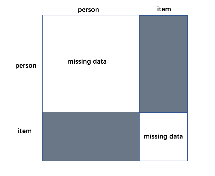
Little statistical theory has been developed for the recovery of configuration based on MDS models. The most relevant work is Zhang et al., 2016, in which an error bound is developed for the recovery of the complete distance matrix, under a linear MDS model without structurally missing data. However, little discussion is provided on the recovery of ideal point configuration, under an MDU setting.

The recovery of configuration is relatively easier under the setting of MDS with no structurally missing data. This is because, the complete data matrix of similarities will provide sufficient information on the complete distance matrix. The accurate recovery of the complete distance matrix further implies the accurate recovery of configuration under weak conditions, due to the one-to-one relationship between the complete distance matrix and the ideal point configuration as described in Proposition 1. Under the MDU setting, the recovery of configuration requires additional regularity conditions, due to the lack of direct measurement of within-set distances.

MDU is also related to other scaling methods for binary data such as item response theory (Embretson and Reise, 2000; Reckase, 2009, IRT;) and multiple correspondence analysis (Gifi, 1990; Le Roux and Rouanet, 2010). Specifically, probabilistic models are available from IRT for multivariate binary data. An IRT model also represents respondents and items by low-dimensional parameter vectors, say $\boldsymbol{\theta}_{i}$ and $\mbox{$\mathbf{a}$}_{j}$. It also assumes that the probability of $Y_{ij}=1$ is a function of $\boldsymbol{\theta}_{i}$ and $\mbox{$\mathbf{a}$}_{j}$. In this sense, the model introduced above can be viewed as a special IRT model, in which the probability of $Y_{ij}=1$ is assumed to be a monotone decreasing function of $\|\boldsymbol{\theta}_{i}-\mbox{$\mathbf{a}$}_{j}\|$. However, the classical IRT models (Embretson and Reise, 2000; Reckase, 2009, see e.g.,) are not specified in this way. Consequently, it does not make sense to visualize the person and item parameter vectors jointly.

Multiple correspondence analysis is an algorithm-based approach that can be applied to binary data and produce low-dimensional scores for both respondents and items. These score vectors can be plotted jointly in the same space. However, as a common issue with algorithm-based approaches, the meaning of the distance between the score vectors is not clear and the uncertainty associated with the visualization is hard to quantify.

We first study the recovery of configuration from a perturbed partial distance matrix, when both $N$ and $J$ grow to infinity. Let $\boldsymbol{\theta}_{i}^{*}$, $i=1,...,N$, and $\mbox{$\mathbf{a}$}_{j}^{*}$, $j=1,...,J$ be the true person and item ideal points in $\mathbb{R}^{K}$, respectively, and let $D^{*}_{N,J}$ be the corresponding partial distance matrix. In addition, let $\tilde{\boldsymbol{\theta}}_{i}\in\mathbb{R}^{K_{+}}$ and $\tilde{\mbox{$\mathbf{a}$}}_{j}\in\mathbb{R}^{K_{+}}$ correspond to a perturbed version of the true configuration, satisfying

and $K_{+}\geq K,$ where $\tilde{D}_{N,J}$ denotes the partial distance matrix given by the perturbed configuration and $\|\cdot\|_{F}$ denotes the matrix Frobenius norm. One can think of $K_{+}$ as the latent dimension of the MDU model being applied to data, and $\tilde{\boldsymbol{\theta}}_{i}$ and $\tilde{\mbox{$\mathbf{a}$}}_{j}$ as some estimates of the person and item ideal points. For the time being, we treat $K_{+}$, $\tilde{\boldsymbol{\theta}}_{i}$, and $\tilde{\mbox{$\mathbf{a}$}}_{j}$ as given.

Based on the definition of matrix Frobenius norm, the left side of (4) has $NJ$ terms, each of which is a squared distance between a true person-item distance and its perturbed value. Equation (4) implies that the perturbed partial distance matrix converges to the true one in an average sense, when both $N$ and $J$ grow to infinity.

We denote $\boldsymbol{\theta}_{i}^{+}=((\boldsymbol{\theta}_{i}^{*})^{\top},\mathbf{0}^{\top})^{\top}$ and $\mbox{$\mathbf{a}$}_{j}^{+}=((\mbox{$\mathbf{a}$}_{j}^{*})^{\top},\mathbf{0}^{\top})^{\top}$ in $\mathbb{R}^{K_{+}}$ as the embedding of the true ideal points in $\mathbb{R}^{K_{+}}$, where $\bf 0$ denotes a zero vector. In what follows, we show that

as $N$ and $J$ grow to infinity, under reasonable conditions on the true ideal points.

Throughout this paper, we assume that ideal points are constrained in a compact set in $\mathbb{R}^{K}$.

• A0.

  There exists a constant $M$ such that $\|\boldsymbol{\theta}_{i}^{*}\|\leq M$ and $\|\mbox{$\mathbf{a}$}_{j}^{*}\|\leq M$ for all $i$ and $j$.

To impose regularity conditions on the true configuration of the $N+J$ ideal points, which can vary with $N$ and $J$, we introduce the notion of anchor points, two finite sets of points in $\mathbb{R}^{K}$ satisfying certain regularities that are independent of $N$ and $J$.

Let $D^{*}=(\|\mathbf{b}_{i}^{*}-\mathbf{c}_{j}^{*}\|^{2})_{k_{1}\times k_{2}}$ be the partial distance matrix based on the anchor points, whose entries are assumed to be all positive (i.e., there is no identical points).

• A1.

  There exists $\eta>0$ such that for any partial distance matrix $D\in\mathbb{R}^{k_{1}\times k_{2}}$ satisfying $\|D-D^{*}\|_{F}<\eta,$ $D$ has a unique configuration.

• A2.

  Both $\{\mathbf{b}_{1}^{*},...,\mathbf{b}_{k_{1}}^{*}\}$ and $\{\mathbf{c}_{1}^{*},...,\mathbf{c}_{k_{2}}^{*}\}$ can affine span $\mathbb{R}^{K}$.

According to condition A1, the anchor points are well-behaved points whose configuration can be uniquely determined by the partial distance matrix, even after a small perturbation. In addition, thanks to A2, the anchor points will help to anchor the rest of the points in $\mathbb{R}^{K}$, i.e., determining the configuration of a larger set of respondent and item ideal points.

Following the above concept of anchor points, it is intuitive that if there exist anchor points $\{\mathbf{b}_{1}^{*},...,\mathbf{b}_{k_{1}}^{*}\}$ and $\{\mathbf{c}_{1}^{*},...,\mathbf{c}_{k_{2}}^{*}\}$, satisfying that each $\mathbf{b}_{i}^{*}$ is surrounded by sufficiently many respondent ideal points and each $\mathbf{c}_{j}^{*}$ is surrounded by sufficiently many item ideal points; that is, there exist a sufficient number of anchor points. Then it is relatively easy to recover the configuration of the ideal points from a perturbed partial distance matrix. This intuition is formalized by condition A3 below.

• A3.

  There exists a collection of anchor points $\{\mathbf{b}_{1}^{*},...,\mathbf{b}_{k_{1}}^{*}\}$ and $\{\mathbf{c}_{1}^{*},...,\mathbf{c}_{k_{2}}^{*}\}\subset B^{K}_{\bf 0}(M)\subset\mathbb{R}^{K}$ and $0<\epsilon<M/10$ such that the closed balls with $\mathbf{b}_{1}^{*},...,\mathbf{b}_{k_{1}}^{*}$ and $\mathbf{c}_{1}^{*},...,\mathbf{c}_{k_{2}}^{*}$ as centers and radius $\epsilon$, denoted by $B_{\mathbf{b}_{1}^{*}}(\epsilon),...,B_{\mathbf{b}_{k_{1}}^{*}}(\epsilon)$ and $B_{\mathbf{c}_{1}^{*}}(\epsilon),...,B_{\mathbf{c}_{k_{2}}^{*}}(\epsilon)$, do not overlap. The following two conditions are required to hold.

  1. (1)

     For any $\mathbf{b}_{1}\in B_{\mathbf{b}_{1}^{*}}(\epsilon),...,\mathbf{b}_{k_{1}}\in B_{\mathbf{b}_{k_{1}}^{*}}(\epsilon)$ and $\mathbf{c}_{1}\in B_{\mathbf{c}_{1}^{*}}(\epsilon),...,\mathbf{c}_{k_{2}}\in B_{\mathbf{c}_{k_{2}}^{*}}(\epsilon)$, $\{\mathbf{b}_{1},...,\mathbf{b}_{k_{1}}\}$ and $\{\mathbf{c}_{1},...,\mathbf{c}_{k_{2}}\}$ are also a collection of anchor points.

  2. (2)

     When $N$ and $J$ grow to infinity,

     		$\displaystyle p_{i}=\liminf\limits_{N\to\infty}\frac{\sum_{l=1}^{N}1_{\{\|\boldsymbol{\theta}^{*}_{l}-\mathbf{b}_{i}^{*}\|<\epsilon\}}}{N}>0,\quad i=1,...,k_{1},$
     		$\displaystyle q_{j}=\liminf\limits_{J\to\infty}\frac{\sum_{l=1}^{J}1_{\{\|\mbox{$\mathbf{a}$}^{*}_{l}-\mathbf{c}_{j}^{*}\|<\epsilon\}}}{J}>0,\quad j=1,...,k_{2}.$

In what follows, we propose a constrained maximum likelihood estimator and show its properties. Given the assumptions of the MDU model, our likelihood function takes the form

Based on this likelihood function, we consider the following estimator

where $K_{+}$ and $M$ are pre-specified. We denote $\hat{D}_{N,J}$ as the partial distance matrix based on $\hat{\boldsymbol{\theta}}_{i}$s and $\hat{\mbox{$\mathbf{a}$}}_{j}$s from (7).

We impose the following regularity condition on the link function $f$, which requires $f$ to be neither too steep nor too flat in the feasible domain. Similar conditions are assumed in Davenport et al., 2014 for solving a 1-bit matrix completion problem.

• A4.

  The link function $f:\mathbb{R}\rightarrow(0,1)$ is a smooth and monotone decreasing function, satisfying $L_{4M^{2}}<\infty$ and $\beta_{4M^{2}}<\infty,$ where

  $$L_{\alpha}=\sup\limits_{|x|\leq\alpha}\frac{|f^{\prime}(x)|}{f(x)(1-f(x))},\mbox{~~and~~}\beta_{\alpha}=\sup\limits_{|x|\leq\alpha}\frac{f(x)(1-f(x))}{|f^{\prime}(x)|^{2}}.$$

Proposition 3 implies that $\|\hat{D}_{N,J}-D_{N,J}^{*}\|_{F}^{2}=o_{p}(NJ)$, which, combined with Theorem 1, leads to Theorem 2 below.

We propose an alternating minimization algorithm for solving (7). To handle the constraints in (7), a projected gradient descent update is used in each iteration. For $\mathbf{x}\in\mathbb{R}^{K_{+}}$, we define the following projection operator:

We further discuss the configuration recovery problem when data have many missing values, which is commonly encountered in practice. Denote matrix $\Omega=(\omega_{ij})_{N\times J}$, where $\omega_{ij}=1$ indicates that response $y_{ij}$ is observed and $\omega_{ij}=0$ indicates $y_{ij}$ is missing. We consider the simple case of uniformly missing, as described in condition A5. We point out that this assumption can be relaxed to analyzing data that have non-uniformly missing entries, following the developments in Cai and Zhou, 2013 for solving a 1-bit matrix completion problem.

• A5.

  Entries of $\Omega$, $\omega_{ij}$, are independent and identically distributed Bernoulli random variables with

  $$P(\omega_{ij}=1)=\frac{n}{NJ}.$$

Under this condition, there are on average $n$ entries of the data matrix $(y_{ij})_{N\times J}$ that are observable. Thanks to the ignorable missingness, given $\Omega$ and the observed data, the likelihood becomes

We still consider a constrained maximum likelihood estimator

Let $\hat{D}_{N,J}^{\Omega}$ denote the partial distance matrix for $\hat{\boldsymbol{\theta}}_{1}^{\Omega},...,\hat{\boldsymbol{\theta}}_{N}^{\Omega},\hat{\mbox{$\mathbf{a}$}}_{1}^{\Omega},...,\hat{\mbox{$\mathbf{a}$}}_{J}^{\Omega}$. Proposition 4 presents a missing-data version of Proposition 3. It implies that we can still recover the partial distance matrix if $n$ is large enough.

References

- Alfakih, (2003) Alfakih, A. Y. (2003). On the uniqueness of euclidean distance matrix completions. Linear Algebra and its Applications, 370:1–14.
- Bach, (2008) Bach, F. R. (2008). Consistency of trace norm minimization. Journal of Machine Learning Research, 9:1019–1048.
- Bai and Ng, (2002) Bai, J. and Ng, S. (2002). Determining the number of factors in approximate factor models. Econometrica, 70:191–221.
- Bakker and Poole, (2013) Bakker, R. and Poole, K. T. (2013). Bayesian metric multidimensional scaling. Political Analysis, 21:125–140.
- Bartholomew et al., (2011) Bartholomew, D. J., Knott, M., and Moustaki, I. (2011). Latent variable models and factor analysis: A unified approach. John Wiley & Sons, West Sussex, UK.
- Bennett, (1956) Bennett, J. F. (1956). Determination of the number of independent parameters of a score matrix from the examination of rank orders. Psychometrika, 21:383–393.
- Bennett and Hays, (1960) Bennett, J. F. and Hays, W. L. (1960). Multidimensional unfolding: Determining the dimensionality of ranked preference data. Psychometrika, 25:27–43.
- Borg and Groenen, (2005) Borg, I. and Groenen, P. J. (2005). Modern multidimensional scaling: Theory and applications. Springer, New York, NY.
- Busing et al., (2005) Busing, F. M., Groenen, P. J., and Heiser, W. J. (2005). Avoiding degeneracy in multidimensional unfolding by penalizing on the coefficient of variation. Psychometrika, 70:71–98.
- Cai and Zhou, (2013) Cai, T. and Zhou, W.-X. (2013). A max-norm constrained minimization approach to 1-bit matrix completion. Journal of Machine Learning Research, 14:3619–3647.
- Chen and Lei, (2018) Chen, K. and Lei, J. (2018). Network cross-validation for determining the number of communities in network data. Journal of the American Statistical Association, 113:241–251.
- Chen and Buja, (2009) Chen, L. and Buja, A. (2009). Local multidimensional scaling for nonlinear dimension reduction, graph drawing, and proximity analysis. Journal of the American Statistical Association, 104:209–219.
- (13) Chen, Y., Fan, J., Ma, C., and Yan, Y. (2019a). Inference and uncertainty quantification for noisy matrix completion. Proceedings of the National Academy of Sciences, 116:22931–22937.
- (14) Chen, Y., Li, X., and Zhang, S. (2019b). Structured latent factor analysis for large-scale data: Identifiability, estimability, and their implications. Journal of the American Statistical Association. (in press).
- Cheney and Kincaid, (2009) Cheney, W. and Kincaid, D. (2009). Linear algebra: Theory and applications. The Australian Mathematical Society, 110:544–550.
- Choi and Wolfe, (2014) Choi, D. and Wolfe, P. J. (2014). Co-clustering separately exchangeable network data. The Annals of Statistics, 42:29–63.
- (17) Clinton, J., Jackman, S., and Rivers, D. (2004a). The statistical analysis of roll call data. American Political Science Review, 98:355–370.
- (18) Clinton, J. D., Jackman, S., and Rivers, D. (2004b). “The most liberal senator”? Analyzing and interpreting congressional roll calls. PS: Political Science & Politics, 37:805–811.
- Coombs, (1964) Coombs, C. H. (1964). A theory of data. Wiley, New York, NY.
- Critchley, (1988) Critchley, F. (1988). On certain linear mappings between inner-product and squared-distance matrices. Linear Algebra and its Applications, 105:91–107.
- Davenport et al., (2014) Davenport, M. A., Plan, Y., van den Berg, E., and Wootters, M. (2014). 1-bit matrix completion. Information and Inference: A Journal of the IMA, 3:189–223.
- de Leeuw, (2005) de Leeuw, J. (2005). Multidimensional unfolding. In Everitt, B. and Howell, D. C., editors, Encyclopedia of statistics in behavioral science. Wiley, London, UK.
- de Leeuw and Mair, (2009) de Leeuw, J. and Mair, P. (2009). Multidimensional scaling using majorization: SMACOF in R. Journal of Statistical Software, 31:1–30.
- DeSarbo and Hoffman, (1987) DeSarbo, W. S. and Hoffman, D. L. (1987). Constructing MDS joint spaces from binary choice data: A multidimensional unfolding threshold model for marketing research. Journal of Marketing Research, 24:40–54.
- DeSarbo et al., (1997) DeSarbo, W. S., Young, M. R., and Rangaswamy, A. (1997). A parametric multidimensional unfolding procedure for incomplete nonmetric preference/choice set data in marketing research. Journal of Marketing Research, 34:499–516.
- Dhillon, (2001) Dhillon, I. S. (2001). Co-clustering documents and words using bipartite spectral graph partitioning. In Proceedings of the seventh ACM SIGKDD international conference on Knowledge discovery and data mining, pages 269–274.
- Donoho and Stodden, (2004) Donoho, D. and Stodden, V. (2004). When does non-negative matrix factorization give a correct decomposition into parts? In Thrun, S., Saul, L., and Schölkopf, B., editors, Advances in neural information processing systems, pages 1141–1148. MIT Press, Cambridge, MA.
- Embretson and Reise, (2000) Embretson, S. E. and Reise, S. P. (2000). Item response theory. Psychology Press, Hove, UK.
- Friedman et al., (2001) Friedman, J., Hastie, T., and Tibshirani, R. (2001). The elements of statistical learning. Springer, New York, NY.
- Gifi, (1990) Gifi, A. (1990). Nonlinear multivariate analysis. Wiley, New York, NY.
- Greenacre and Browne, (1986) Greenacre, M. J. and Browne, M. W. (1986). An efficient alternating least-squares algorithm to perform multidimensional unfolding. Psychometrika, 51:241–250.
- Harper and Konstan, (2016) Harper, F. M. and Konstan, J. A. (2016). The movielens datasets: History and context. ACM Transactions on Interactive Intelligent Systems (TiiS), 5:1–19.
- Hartigan, (1972) Hartigan, J. A. (1972). Direct clustering of a data matrix. Journal of the American Statistical Association, 67:123–129.
- Hays and Bennett, (1961) Hays, W. L. and Bennett, J. F. (1961). Multidimensional unfolding: Determining configuration from complete rank order preference data. Psychometrika, 26:221–238.
- Hinich, (2005) Hinich, M. J. (2005). A new method for statistical multidimensional unfolding. Communications in Statistics—Theory and Methods, 34:2299–2310.
- Ho et al., (2010) Ho, Y., Chung, Y., and Lau, K. (2010). Unfolding large-scale marketing data. International Journal of Research in Marketing, 27:119–132.
- Holland et al., (1983) Holland, P. W., Laskey, K. B., and Leinhardt, S. (1983). Stochastic blockmodels: First steps. Social Networks, 5:109–137.
- Hoyer, (2004) Hoyer, P. O. (2004). Non-negative matrix factorization with sparseness constraints. Journal of machine learning research, 5:1457–1469.
- Kruskal, (1964) Kruskal, J. B. (1964). Multidimensional scaling by optimizing goodness of fit to a nonmetric hypothesis. Psychometrika, 29:1–27.
- Kruskal and Wish, (1978) Kruskal, J. B. and Wish, M. (1978). Multidimensional scaling. Sage, Beverly Hills, CA.
- Le Roux and Rouanet, (2010) Le Roux, B. and Rouanet, H. (2010). Multiple correspondence analysis. Sage, Newbury Park, CA.
- Li et al., (2020) Li, T., Levina, E., and Zhu, J. (2020). Network cross-validation by edge sampling. Biometrika, 107:257–276.
- Lu et al., (2005) Lu, F., Keleş, S., Wright, S. J., and Wahba, G. (2005). Framework for kernel regularization with application to protein clustering. Proceedings of the National Academy of Sciences, 102:12332–12337.
- MacQueen, (1967) MacQueen, J. (1967). Some methods for classification and analysis of multivariate observations. In Cam, L. M. L. and Neyman, J., editors, Proceedings of the fifth Berkeley symposium on mathematical statistics and probability, pages 281–297. University of California Press, Berkeley, CA.
- Mair et al., (2016) Mair, P., Borg, I., and Rusch, T. (2016). Goodness-of-fit assessment in multidimensional scaling and unfolding. Multivariate Behavioral Research, 51:772–789.
- Olver, (1999) Olver, P. J. (1999). Classical invariant theory. Cambridge University Press, Cambridge, UK.
- Papesh and Goldinger, (2010) Papesh, M. H. and Goldinger, S. D. (2010). A multidimensional scaling analysis of own- and cross-race face spaces. Cognition, 116:283–288.
- Poole, (2000) Poole, K. T. (2000). Nonparametric unfolding of binary choice data. Political Analysis, 8:211–237.
- Poole, (2005) Poole, K. T. (2005). Spatial models of parliamentary voting. Cambridge University Press, Cambridge, UK.
- Poole and Rosenthal, (1991) Poole, K. T. and Rosenthal, H. (1991). Patterns of congressional voting. American Journal of Political Science, 35:228–278.
- Poole et al., (1991) Poole, K. T., Rosenthal, H., and Koford, K. (1991). On dimensionalizing roll call votes in the US congress. American Political Science Review, 85:955–976.
- Rabe-Hesketh and Skrondal, (2004) Rabe-Hesketh, S. and Skrondal, A. (2004). Generalized latent variable modeling: Multilevel, longitudinal, and structural equation models. Chapman and Hall/CRC, New York, NY.
- Reckase, (2009) Reckase, M. (2009). Multidimensional Item Response Theory. Springer, New York, NY.
- Rohe et al., (2016) Rohe, K., Qin, T., and Yu, B. (2016). Co-clustering directed graphs to discover asymmetries and directional communities. Proceedings of the National Academy of Sciences, 113:12679–12684.
- Samejima, (1997) Samejima, F. (1997). Graded response model. In van der Linden, W. J. and Hambleton, R. K., editors, Handbook of modern item response theory, pages 85–100. Springer, New York, NY.
- Takane et al., (1977) Takane, Y., Young, F. W., and De Leeuw, J. (1977). Nonmetric individual differences multidimensional scaling: An alternating least squares method with optimal scaling features. Psychometrika, 42:7–67.
- Tenenbaum et al., (2000) Tenenbaum, J. B., De Silva, V., and Langford, J. C. (2000). A global geometric framework for nonlinear dimensionality reduction. Science, 290:2319–2323.
- Van Deun et al., (2007) Van Deun, K., Heiser, W. J., and Delbeke, L. (2007). Multidimensional unfolding by nonmetric multidimensional scaling of Spearman distances in the extended permutation polytope. Multivariate Behavioral Research, 42:103–132.
- Xia and Yuan, (2019) Xia, D. and Yuan, M. (2019). Statistical inferences of linear forms for noisy matrix completion. arXiv preprint arXiv:1909.00116.
- Zhang et al., (2016) Zhang, L., Wahba, G., and Yuan, M. (2016). Distance shrinkage and Euclidean embedding via regularized kernel estimation. Journal of the Royal Statistical Society: Series B (Statistical Methodology), 78:849–867.