跳到论文正文
W Papers独立论文阅读器 arXiv:2009.01514 论文正文 计算阅读时间 · 0%
引用这篇论文根据当前论文元数据生成,正式投稿前建议核对。


License: arXiv.org perpetual non-exclusive license
arXiv:2009.01514v2 [math.NA] 27 Sep 2021

Kernel Interpolation of High Dimensional Scattered DataThanks: August 11, 2026.

Shao-bo Lin Email: sblin1983@gmail.com Thanks: Center for Intelligent Decision-Making and Machine Learning, School of Management, Xi’an Jiaotong University, Xi’an 710049, China ().    Xiangyu Chang Email: xiangyuchang@xjtu.edu.cn Thanks: Center for Intelligent Decision-Making and Machine Learning, School of Management, Xi’an Jiaotong University, Xi’an 710049, China ().    Xingping Sun Email: XSun@MissouriState.edu Thanks:  Department of Mathematics, Missouri State University, Springfield, MO 65897, USA ().
Abstract

Data sites selected from modeling high-dimensional problems often appear scattered in non-paternalistic ways. Except for sporadic-clustering at some spots, they become relatively far apart as the dimension of the ambient space grows. These features defy any theoretical treatment that requires local or global quasi-uniformity of distribution of data sites. Incorporating a recently-developed application of integral operator theory in machine learning, we propose and study in the current article a new framework to analyze kernel interpolation of high dimensional data, which features bounding stochastic approximation error by the spectrum of the underlying kernel matrix. Both theoretical analysis and numerical simulations show that spectra of kernel matrices are reliable and stable barometers for gauging the performance of kernel-interpolation methods for high dimensional data.

keywords
High dimension, kernel interpolation, random sampling, stochastic approximation
Funding.
The first two authors of the article are partially supported by the National Natural Science Foundation of China [Grant Nos. 61876133,11771012].
††runningheads: Kernel Interpolation of High Dimensional Scattered Data / S.-B. Lin, X. Chang, and X.Sun
AMS
68T05, 94A20, 41A35

1 Introduction

Let 𝒳\mathcal{X} be a compact domain in ℝd\mathbb{R}^{d} with Lipschitz boundary. Let K⁡(⋅,⋅):𝒳×𝒳→ℝK(\cdot,\cdot):{\mathcal{X}}\times{\mathcal{X}}\rightarrow\mathbb{R} be a continuous, symmetric and strictly positive-definite kernel. Suppose that a data set D:={(xi,yi)}i=1mD:=\{(x_{i},y_{i})\}_{i=1}^{m} is given, in which Ξ:={xi}i=1m\Xi:=\{x_{i}\}_{i=1}^{m} are mm scattered points from 𝒳\mathcal{X}, and {yi}i=1m\{y_{i}\}_{i=1}^{m} are values of a target function ff taken on Ξ\Xi. In employing a kernel method to model a real world problem, one designs or adopts an algorithm to select an fD∈KΞ:=span​{Kxj}i=1mf_{D}\in K_{\Xi}:={\rm span}\{K_{x_{j}}\}_{i=1}^{m}, which represents “faithfully” the target function ff on 𝒳\mathcal{X}. Here KxjK_{x_{j}} denotes the function: 𝒳∋x↦K⁡(xj,x)\mathcal{X}\ni x\mapsto K(x_{j},x). While the selection of an algorithm is subject to practical constraints and (possibly) subjective bias, and criteria for the faithfulness of the representation are up to improvising, veracity, and (even) debate, the approximation capability of the subspace KΞK_{\Xi} is always at the core of every theoretical consideration. In a reproducing kernel Hilbert Space (RKHS) setting (often referred to as a native space in the approximation theory community), the best approximation from the subspace KΞK_{\Xi} is achieved via interpolation. That is, one chooses fD∈KΞ,f_{D}\in K_{\Xi}, such that fD(xj)=yj,j=1,…,m,f_{D}(x_{j})=y_{j},\;j=1,\ldots,m, which can be precisely written as the following:

fD=∑i=1mai​Kxi,in which(a1,…,am)T=𝕂−1​yD.f_{D}=\sum_{i=1}^{m}a_{i}K_{x_{i}},\quad\mbox{in which}\quad(a_{1},\dots,a_{m})^{T}=\mathbb{K}^{-1}y_{D}. (1)

Here 𝕂=(K⁡(xi,xj))i,j=1m\mathbb{K}=(K(x_{i},x_{j}))_{i,j=1}^{m} denotes the interpolation matrix (also called kernel matrix), and yD=(y1,…,ym)Ty_{D}=(y_{1},\dots,y_{m})^{T}. For some radial basis kernels, such as thin plate splines, approximation power can transcend a native space barrier so that a “near best” approximation order be realized for functions from a larger (than the native space) RKHS. For readers who are interested in the above native space approximation narrative, we make reference to [26, 29, 30, 31, 32, 28, 33, 37, 38, 43], and the bibliographies therein.

Hangelbroek et al ([14, 15, 16]) have recently made significant advancement in expanding the approximation power of interpolation beyond the native space setting, a gist of which will be summarized as follows. Let

hΞ:=maxx∈𝒳⁡min1≤j≤m⁡d⁡(xj,x),qΞ=12​minj≠k⁡d⁡(xj,xk).h_{\Xi}:=\max_{x\in\mathcal{X}}\min\limits_{1\leq j\leq m}d(x_{j},x),\quad q_{\Xi}=\frac{1}{2}\min\limits_{j\neq k}d(x_{j},x_{k}).

The former is the Hausdorff distance between the point set Ξ\Xi and 𝒳\mathcal{X}, but is more commonly referred to in the literature as mesh norm or fill-distance; the latter is the separation radius (or half of the minimal separation) of the point set Ξ\Xi. If there is a constant 1≤Cd1\leq C_{d} depending only on dd, such that hΞ/qΞ≤Cdh_{\Xi}/q_{\Xi}\leq C_{d}, then we say that the point set Ξ\Xi is quasi-uniformly distributed in 𝒳\mathcal{X}. Global or local quasi-uniformity of a data set Ξ\Xi is a crucial analytical tool for meshless kernel methods to achieve their approximation goals. In particular, approximation orders of meshless kernel methods are mostly given in terms of hΞh_{\Xi}.

Let Ω\Omega be a dd-dimensional Riemannian manifold. Let Ξ∗\Xi^{*} be a discrete subset of Ω\Omega that is quasi-uniformly distributed in Ω\Omega. Let χξ\chi_{\xi} be the Lagrange interpolating function headquartered at ξ\xi and associated with the surface splines or the Matérn kernel. That is χξ​(ζ)=δξ,ζ,ξ,ζ∈Ξ∗,\chi_{\xi}(\zeta)=\delta_{\xi,\zeta},\;\xi,\zeta\in\Xi^{*}, where δξ,ζ\delta_{\xi,\zeta} is the Kronecker delta. Hangelbroek, Narcowich, and Ward [15] established the following remarkable inequality:

|χξ​(x)|≤C⁡(d)​exp⁡[−ν⁡(d)​dist⁡(x,ξ)hΞ∗],x∈Ω.|\chi_{\xi}(x)|\leq C(d)\exp\left[-\nu(d)\frac{{\rm dist}(x,\xi)}{h_{\Xi^{*}}}\right],\quad x\in\Omega. (2)

Here C⁡(d),ν⁡(d)>0C(d),\nu(d)>0 are constants depending only on dd and the underlying kernels. However, both constants grow at an exponential rate with respect to dd. They further showed that the interpolation operator is bounded from Cp​(Ω)C_{p}(\Omega) to itself, where Cp​(Ω)C_{p}(\Omega) denotes the totality of continuous functions on Ω\Omega with polynomial growth at infinity. In a follow up article, Hangelbroek et al [14] proved that the L2L^{2}-projector is bounded under the L∞L^{\infty}-norm. Leveraging the exponential decay of χξ\chi_{\xi} away from the base point ξ\xi as shown in inequality (2), Hangelbroek, Narcowich, and Ward [16] and Fuselier et al [10] articulated the notion “local density function” in which Lagrange interpolating functions are built on data sets whose cardinality are of logarithmic orders, and yet the interpolation scheme still achieves desirable approximation orders. This has vastly reduced computational complexity, and enhanced the efficiency of many meshless methods in solving partial differential equations on domains of relatively low dimensions; see [13].

Modern-day data scientists are encountering an onslaught of real world problems in which massive data sets are involved. In many cases, data seem extremely disorganized and even outright chaotic, which not only poses challenges but also provides opportunities for data scientists to figure out ways to store, communicate and analyze them. A persisting challenge stems from experiences in dealing with the enormous number of features (variables) data sets exhibit. For example, microarrays for gene expression [2] contain thousands of samples, each of which in turn has tens of thousands of genes. Another well-known example is the natural image data set - ImageNet [9], which gathers about 14 million natural images classified in more than 20,000 categories. Each image has the original resolution with 469×387=1,823,003469\times 387=1,823,003 pixels (dimensions). Our numerical simulations show that high dimensional data sites may exhibit sporadic-clustering at some spots, but are mostly scattered in non paternalistic ways and relatively far apart from each other, which defies any attempt to analyze them using the likes of local density functions.

Suppose that mass is uniformly distributed on [0,1]d[0,1]^{d}, the unit cube in ℝd\mathbb{R}^{d}. Then for any fixed 0<ϵ<12,0<\epsilon<\frac{1}{2}, and a sufficiently large dd, the law of large numbers shows that the mass of [0,1]d[0,1]^{d} is mostly concentrated in an ϵ\epsilon-neighbourhood of the hyperplane ℒ:x1+⋯+xd=d2\mathcal{L}:x_{1}+\cdots+x_{d}=\frac{d}{2}, which happens to be the orthogonal bisector of the main diagonal of [0,1]d[0,1]^{d} (which has length d\sqrt{d}). Meanwhile the cube [ϵ,1−ϵ]d[\epsilon,1-\epsilon]^{d} has volume (1−2​ϵ)d(1-2\epsilon)^{d}, which approaches zero exponentially fast with dd. Thus, the mass of [0,1]d[0,1]^{d} is mostly concentrated on the intersection of ϵ\epsilon-neighbourhood of the hyperplane ℒ\mathcal{L} and the set [0,1]d∖[ϵ,1−ϵ]d[0,1]^{d}\setminus[\epsilon,1-\epsilon]^{d}. Figure 1 depicts the situation for d=3d=3.

Refer to caption
Figure 1: Concentration of mass on the unit cube.

Figure 2 exhibits the increase of the separation radius qΞq_{\Xi} with dd for random samplings of 500500 points from [0,1]d[0,1]^{d} (according to the uniform distribution). In Figure 2, each red dot indicates the mean values (in 1010 trials) of separation radius for each dimension dd in the range 2≤d≤1002\leq d\leq 100. Each red dot is accompanied with an error bar, indicating the range of variation of separation radius from these trials as determined by the double standard deviation. To further demonstrate the potency of our main methodology undertaken here, we have designed and carried out the following large scale numerical simulation. For each given dimension dd in the range 2≤d≤1002\leq d\leq 100, we first randomly select (according the uniform distribution on [0,1]d[0,1]^{d}) 500500 points x1,…,x500.x_{1},\ldots,x_{500}. We then calculate the condition number (associated with the ℓ2\ell^{2}-norm) of the corresponding kernel matrix 𝕂:=(G⁡(xi,xj))∈ℝ500×500\mathbb{K}:=(G(x_{i},x_{j}))\in\mathbb{R}^{500\times 500}, where G(x,y)=exp{−∥x−y∥2/2}.G(x,y)=\exp\{-\|x-y\|^{2}/2\}. Figure 2 shows that the condition number of 𝕂\mathbb{K} decays exponentially fast to one as dd increases from 22 to 100100. Similar to Figure 2 (a), each red dot indicates the mean value (in 10 trials) of the condition number of 𝕂\mathbb{K} for the corresponding dimension dd, and the accompanied error bar indicates the double standard deviation. 11 1 We have repeated the same simulation many times, and got more or less the same result. This has motivated us to establish probabilistic lower bounds of qXq_{X} in terms of mm and dd; see Lemma 24 (in Appendix C).

Figure 2: The change of random separation radii and condition numbers as dimension increases.

The main goal of the current paper is to propose and study a new stochastic framework for kernel interpolation of high dimensional data. Inspired by our numerical simulation results and Peetre’s idea [34] in the study of interpolation of operators, we introduce two quantities (parameters) in Equations (11) and (12), and use them to bound the error of stochastic approximation for the underlying kernel interpolants. By fine-tuning the two parameters, we observe a KK-functional of a hybrid (continuous and discrete) nature. We think the mathematical lineage interesting, and will investigate deeper connections in the future.

Based on the recently-developed integral operator theory [41, 22, 23], we first express the approximation error as the difference between integral operators and the corresponding empirical discretizations. We then formulate the difference in terms of the spectrum of the kernel matrix. Finally, we employ pertinent concentration inequalities [35] in Banach spaces to derive the desired error estimates (Theorems 9 and 10). Working behind the scene are spectrum estimates of kernel matrix [3, 29, 37, 43, 18, 4, 21], of which we mention particularly that in Ball’s estimate [3] of the smallest eigenvalue of distance matrices in terms of the minimal separation between the data sites, the constant grows algebraically with dimension.

To demonstrate the versatility of our method, we derive stochastic approximation errors for kernel interpolation under three different computing environments. Firstly, we establish a close relationship between approximation error and spectrum of the kernel matrix for noise-free data, that is, D={(xi,yi)}i=1mD=\{(x_{i},y_{i})\}_{i=1}^{m} with yi=f∗​(xi)y_{i}=f^{*}(x_{i}) for f∗∈ℋKf^{*}\in\mathcal{H}_{K}, where ℋK\mathcal{H}_{K} is the RKHS associated with KK. Secondly, we study the performance of kernel interpolation with the presence of noise. Under the circumstance, the data {yi}i=1m\{y_{i}\}_{i=1}^{m} are of the form: yi=f∗​(xi)+εiy_{i}=f^{*}(x_{i})+\varepsilon_{i} in which f∗∈ℋKf^{*}\in\mathcal{H}_{K} and εi\varepsilon_{i} indicate some white noise. Our result shows that there is a trade-off between accuracy of approximation and stability of the underlying algorithm in terms of kernel selections. Finally, we investigate the approximation capability of kernel interpolation beyond the native space setting, assuming that data come from a target function outside of the native space, which we will refer to as “trans-native space data”. This is figuratively called “conquering the native space barrier” in [28].

The rest of paper is organized as follows. In Section 2, we outline the integral operator approach, which is a theoretical pillar of the current article, and establish the relationship between the approximation error and the norm estimate of the corresponding integral operator. In Section 3, we formulate the approximation error of kernel interpolation in terms of the spectrum of kernel matrix. In Section 4, we give spectrum estimates for some widely used kernels and remarks on the implication for the ensuing sampling and interpolating operations. In Section 5, we report some numerical simulation results. In Section 6, we present the proofs of our results. Not to distract readers’ attention from the main narrative, we collect some frequently-used results in three appendices for easy referencing.

2 Error Analysis for Kernel Interpolation via Finite Differences of Operators

This section features a novel integral operator approach to analyze the approximation performance of kernel interpolation. Prototypical ideas of this approach already appeared in [39, 40, 22]. Let ρX\rho_{X} be a probability measure on 𝒳\mathcal{X}. Denote by LρX2L^{2}_{\rho_{X}} the space of ρX\rho_{X}-square-integrable functions endowed with norm ∥⋅∥ρ\|\cdot\|_{\rho}. Define the integral operator LK:ℋK→ℋKL_{K}:\mathcal{H}_{K}\rightarrow\mathcal{H}_{K} by

LK​(f)=∫𝒳Kx​f​(x)​d​ρX,f∈ℋK.L_{K}(f)=\int_{\mathcal{X}}K_{x}f(x)d\rho_{X},\qquad f\in{\mathcal{H}}_{K}. (3)

Let ℒK:LρX2→LρX2\mathcal{L}_{K}:L_{\rho_{X}}^{2}\rightarrow L_{\rho_{X}}^{2} be the integral operator defined by

ℒK​f=∫𝒳f⁡(x)​Kx​d​ρX,f∈LρX2.\mathcal{L}_{K}f=\int_{\mathcal{X}}f(x)K_{x}d\rho_{X},f\in L_{\rho_{X}}^{2}.

We have of course that ℒK​f=LK​f\mathcal{L}_{K}f=L_{K}f for f∈ℋKf\in\mathcal{H}_{K}. However, one can neither consider ℒK\mathcal{L}_{K} an extension of LKL_{K} from HKH_{K} to LρX2L_{\rho_{X}}^{2} nor LKL_{K} a restriction of ℒK\mathcal{L}_{K} on HKH_{K}, as the norms of two spaces are not equivalent (when restricted to LKL_{K}). In fact, for an arbitrary f∈LρX2f\in L_{\rho_{X}}^{2}, we have (see [8]) that ‖f‖ρ=‖ℒK1/2​f‖K\|f\|_{\rho}=\|\mathcal{L}_{K}^{1/2}f\|_{K}, where ℒKr​(r>0)\mathcal{L}_{K}^{r}\ (r>0) is defined by spectral calculus and ‖f‖K\|f\|_{K} denotes the norm of the RKHS ℋK\mathcal{H}_{K}. Let SD:ℋK→ℝmS_{D}:\mathcal{H}_{K}\rightarrow\mathbb{R}^{m} be the sampling operator defined by

SD​f:=(f⁡(xi))i=1m.S_{D}f:=(f(x_{i}))_{i=1}^{m}.

Its scaled adjoint SDT:ℝm→ℋKS_{D}^{T}:\mathbb{R}^{m}\rightarrow\mathcal{H}_{K} is given by

SDT​𝐜:=1m​∑i=1mci​Kxi,𝐜:=(c1,c2,…,cm)T∈ℝm.S_{D}^{T}{\bf c}:=\frac{1}{m}\sum_{i=1}^{m}c_{i}K_{x_{i}},\qquad{\bf c}:=(c_{1},c_{2},\dots,c_{m})^{T}\in\mathbb{R}^{m}.

Then, we have

1m​𝕂=SD​SDT.\frac{1}{m}\mathbb{K}=S_{D}S_{D}^{T}. (4)

This together with (1) implies

fD=SDT​(SD​SDT)−1​yD.f_{D}=S_{D}^{T}(S_{D}S_{D}^{T})^{-1}y_{D}. (5)

We carry out error analysis for the following three computing environments: (i) noise-free data in the native space setting; (ii) noisy-data in the native space setting; (iii) trans-native space data. En route we will frequent some definitions and theorems pertaining to operator theory, which we collect in Appendix A for easy referencing.

2.1 Kernel interpolation of noise-free data

In this subsection, we study the approximation error of fDf_{D} defined by (1) when the data are noise-free, i.e., there exists a function f∗∈LρX2f^{*}\in L^{2}_{\rho_{X}} such that

yi=f∗​(xi).y_{i}=f^{*}(x_{i}). (6)

Define the empirical version of the integral operator LKL_{K} to be

LK,D​f:=SDT​SD​f=1m​∑i=1mf⁡(xi)​Kxi.L_{K,D}f:=S_{D}^{T}S_{D}f=\frac{1}{m}\sum_{i=1}^{m}f(x_{i})K_{x_{i}}.

Since KK is strictly positive definite, LK,DL_{K,D} is a positive operator of rank mm. Denote by {(σℓD,ϕℓD)}ℓ=1∞\{(\sigma_{\ell}^{D},\phi_{\ell}^{D})\}_{\ell=1}^{\infty} the normalized eigen-pairs of LK,DL_{K,D} with σ1D≥σ2D≥⋯≥σmD>0\sigma_{1}^{D}\geq\sigma_{2}^{D}\geq\dots\geq\sigma_{m}^{D}>0 and σm+jD=0\sigma_{m+j}^{D}=0 for j≥1j\geq 1. In the following proposition, we show that fD−f∗f_{D}-f^{*} is in the null space of the operator LK,DL_{K,D}.

Proposition 1.

If D={(xi,yi)i=1mD=\{(x_{i},y_{i})_{i=1}^{m} satisfies (6), then f∗−fDf^{*}-f_{D} is in the null space of the operator LK,DL_{K,D}, i.e.

LK,D​(f∗−fD)=0.L_{K,D}(f^{*}-f_{D})=0. (7)

Proposition 1 implies for any ν≥1/2\nu\geq 1/2 that

‖LK,Dν​(f∗−fD)‖K2\displaystyle\|L_{K,D}^{\nu}(f^{*}-f_{D})\|_{K}^{2} =\displaystyle= ⟨LK,Dν​(f∗−fD),LK,Dν​(f∗−fD)⟩K\displaystyle\langle L_{K,D}^{\nu}(f^{*}-f_{D}),L_{K,D}^{\nu}(f^{*}-f_{D})\rangle_{K} (8)
=\displaystyle= ⟨LK,D​(f∗−fD),LK,D2​ν−1​(f∗−fD)⟩K=0.\displaystyle\langle L_{K,D}(f^{*}-f_{D}),L_{K,D}^{2\nu-1}(f^{*}-f_{D})\rangle_{K}=0.

To quantitatively describe the approximation performance of fDf_{D}, some regularity of the target function f∗f^{*} should be imposed. We adopt the widely used regularity assumption [8, 22, 25] via the integral operator ℒK\mathcal{L}_{K}.

f∗=ℒKr​h∗,h∗∈LρX2,r≥0.f^{*}=\mathcal{L}_{K}^{r}h^{*},\qquad\ h^{*}\in L_{\rho_{X}}^{2},\ r\geq 0. (9)

Let {(σℓ,ϕℓ)}ℓ=1∞\{(\sigma_{\ell},\phi_{\ell})\}_{\ell=1}^{\infty} be the normalized eigen-pairs of LKL_{K} with σ1≥σ2≥⋯≥0\sigma_{1}\geq\sigma_{2}\geq\dots\geq 0. Then Aronszajn thoerem [1] shows that {(σℓ,ϕℓ/σℓ)}ℓ=1∞\{(\sigma_{\ell},\phi_{\ell}/\sqrt{\sigma_{\ell}})\}_{\ell=1}^{\infty} consists an normalized eigen-paris of ℒK\mathcal{L}_{K}. Furthermore, the Mercer expansion [1] shows

K⁡(x,x′)=∑ℓ=1∞ϕℓ​(x)​ϕℓ​(x′)=∑ℓ=1∞σℓ​ϕℓ​(x)σℓ​ϕℓ​(x′)σℓK(x,x^{\prime})=\sum_{\ell=1}^{\infty}\phi_{\ell}(x)\phi_{\ell}(x^{\prime})=\sum_{\ell=1}^{\infty}\sigma_{\ell}\frac{\phi_{\ell}(x)}{\sqrt{\sigma_{\ell}}}\frac{\phi_{\ell}(x^{\prime})}{\sqrt{\sigma_{\ell}}}

Then the regularity condition (9) is equivalent to

f∗=ℒKr​h∗=∑ℓ=1∞σℓr−1/2​⟨h∗,ϕℓ/σℓ⟩ρ​ϕℓ.f^{*}=\mathcal{L}_{K}^{r}h^{*}=\sum_{\ell=1}^{\infty}\sigma^{r-1/2}_{\ell}\langle h^{*},\phi_{\ell}/\sqrt{\sigma_{\ell}}\rangle_{\rho}\phi_{\ell}. (10)

This means that the parameter rr in (9) determines the smoothness of the target functions. In particular, (9) with r=1/2r=1/2 implies f∗∈ℋKf^{*}\in\mathcal{H}_{K}, (9) with r<1/2r<1/2 implies f∗∉ℋKf^{*}\notin\mathcal{H}_{K} and (9) with r=0r=0 yields fρ∈LρX2f_{\rho}\in L_{\rho_{X}}^{2}. Generally speaking, the larger value of rr is, the smoother the function f∗f^{*} is. There is a rich literature devoted to characterizing the smoothness of functions in terms of the decay rate of eigenvalue sequence of the associated compact positive operators; see Weyl [44], Kühn[19], Reade [36], and the references therein.

As the regularity is described via LKL_{K} while fD−f∗f_{D}-f^{*} is in the null space of LK,DL_{K,D}, we introduce two quantities to measure the difference between LKL_{K} and LK,DL_{K,D}. For any λ>0\lambda>0, write

𝒬D,λ\displaystyle\mathcal{Q}_{D,\lambda} :⁣=\displaystyle:= ‖(LK,D+λI)−1/2(LK+λI)1/2‖,\displaystyle\left\|(L_{K,D}+\lambda I)^{-1/2}(L_{K}+\lambda I)^{1/2}\right\|, (11)
ℛD\displaystyle\mathcal{R}_{D} :⁣=\displaystyle:= ‖LK,D−LK‖H​S,\displaystyle\|L_{K,D}-L_{K}\|_{HS}, (12)

where ‖A‖\|A\| and ‖A‖H​S\|A\|_{HS} denote, respectively, the spectral norm and Hilbert-Schmidt norm of the operator AA. We impose the interpolation condition (6), and use two quantities: 𝒬D,λ\mathcal{Q}_{D,\lambda} and ℛD\mathcal{R}_{D} to bound the approximation error of kernel interpolants. A suitable combination of the two quantities above can be loosely interpreted as a hybrid (discrete and continuous) version of the “KK-functional” introduced by Peetre [34] in the context of operator interpolations. Based on the above preliminaries, we are in a position to present our error estimate in the following theorem.

Theorem 2.

Let 0<u≤1/20<u\leq 1/2. Suppose that D={(xi,yi)}i=1mD=\{(x_{i},y_{i})\}_{i=1}^{m} satisfies (6) and that f∗f^{*} satisfies (9) with r≥1/2r\geq 1/2. Then we have

‖LKu​(fD−f∗)‖K≤minλ>0⁡{λr+u−1/2​𝒬D,λ2​r+2​u−1​‖h∗‖ρ,1/2≤r≤1,(r−1/2)​κr−3/2​‖h∗‖ρ​λu​𝒬D,λ​ℛD,r>1,\|L_{K}^{u}(f_{D}-f^{*})\|_{K}\leq\min_{\lambda>0}\left\{\begin{array}[]{ll}\lambda^{r+u-1/2}\mathcal{Q}_{D,\lambda}^{2r+2u-1}\|h^{*}\|_{\rho},&\quad 1/2\leq r\leq 1,\\ (r-1/2)\kappa^{r-3/2}\|h^{*}\|_{\rho}\lambda^{u}\mathcal{Q}_{D,\lambda}\mathcal{R}_{D},&\quad r>1,\end{array}\right. (13)

where κ=supx,x′∈𝒳K⁡(x,x′)\kappa=\sqrt{\sup_{x,x^{\prime}\in\mathcal{X}}K(x,x^{\prime})}.

Since 𝒳\mathcal{X} is compact, it is easy to check that κ<∞\kappa<\infty, which implies ‖f‖∞≤κ​‖f‖K\|f\|_{\infty}\leq\kappa\|f\|_{K}. This together with ‖f‖ρ=‖ℒK1/2​f‖K\|f\|_{\rho}=\|\mathcal{L}_{K}^{1/2}f\|_{K} shows that (13) includes error estimates under both LρX2L_{\rho_{X}}^{2} norm and L∞L^{\infty} norm for u=1/2u=1/2 and u=0u=0, respectively. In particular, Theorem 2 with u=1/2u=1/2 and r=1/2r=1/2 yields the following corollary.

Corollary 3.

Suppose that D={(xi,yi)}i=1mD=\{(x_{i},y_{i})\}_{i=1}^{m} satisfies (6) and f∗∈ℋKf^{*}\in\mathcal{H}_{K}. Then we have

‖fD−f∗‖ρ≤minλ>0⁡λ1/2​𝒬D,λ​‖h∗‖ρ.\|f_{D}-f^{*}\|_{\rho}\leq\min_{\lambda>0}\lambda^{1/2}\mathcal{Q}_{D,\lambda}\|h^{*}\|_{\rho}.

As shown in the above corollary, if f∗∈ℋKf^{*}\in\mathcal{H}_{K}, a standard assumption in approximation theory [14, 30, 31] and learning theory [8, 41, 22], the approximation rate depends only on 𝒬D,λ\mathcal{Q}_{D,\lambda}, the difference between LKL_{K} and its discretion counterpart. Generally speaking, the mentioned difference in 𝒬D,λ\mathcal{Q}_{D,\lambda} decreases with respect to λ\lambda, making the minimization in Corollary 3 be well definied. Theorem 2 with u=0u=0 and r>1r>1 and ‖LK‖≤κ\|L_{K}\|\leq\kappa and λ=1\lambda=1 can also yield the following error estimate under the L∞​(𝒳)L^{\infty}(\mathcal{X}) norm.

Corollary 4.

Suppose that D={(xi,yi)}i=1mD=\{(x_{i},y_{i})\}_{i=1}^{m} satisfies (6) and that f∗f^{*} satisfies (9) with r>1r>1. Then we have

‖fD−f∗‖∞≤(r−1/2)​(κ+1)r​‖h∗‖ρ​ℛD.\|f_{D}-f^{*}\|_{\infty}\leq(r-1/2)(\kappa+1)^{r}\|h^{*}\|_{\rho}\mathcal{R}_{D}.

All the above results show that the approximation error of kernel interpolation depends heavily on the differences of operators LKL_{K} and LK,DL_{K,D} and is independent of the dimension of input space 𝒳\mathcal{X}. This makes our error analysis totally different from the classical results [30, 31, 13, 15, 43] which introduced the distribution of scattered data such as the mesh norm, separation radius and mesh ratio to quantify the error.

2.2 Kernel interpolation of noisy-data

In this part, we study the approximation performance of kernel interpolation when the data are noisy, that is, there exists an f∗f^{*} satisfying (9) with r≥1/2r\geq 1/2 such that

yi=f∗​(xi)+εi,y_{i}=f^{*}(x_{i})+\varepsilon_{i}, (14)

where εi\varepsilon_{i} satisfies E⁡[εi]=0E[\varepsilon_{i}]=0 and |εi|≤γ|\varepsilon_{i}|\leq\gamma for some γ≥0\gamma\geq 0. It should be mentioned that our noisy model (14) is different from the classical setting [43, 17] that is only available to extremely small noise. In fact, the magnitude of noise in (14) can be comparable with ‖f∗‖∞\|f^{*}\|_{\infty}. Instead, we assume the noise to be randomly white noise, which is standard in statistics and learning theory [8, 21, 24].

The approximation error analysis for (14) is much more sophisticated than the noise-free model (6) which requires the kernel matrix to be well-conditioned. To gauge the effect of noise, we introduce the following quantity:

𝒫D,λ:=‖(LK+λI)−1/2(LK,Df∗−SDTyD)‖K.\displaystyle\mathcal{P}_{D,\lambda}:=\left\|(L_{K}+\lambda I)^{-1/2}(L_{K,D}f^{*}-S_{D}^{T}y_{D})\right\|_{K}. (15)

By the aid of the restriction of εi\varepsilon_{i}, i.e., E⁡[εi]=0E[\varepsilon_{i}]=0, LK,D​f∗L_{K,D}f^{*} can be regarded as a population of SDT​yDS_{D}^{T}y_{D} in terms that

LK,D​f∗−SDT​yD=1m​∑i=1mεi​Kxi.L_{K,D}f^{*}-S_{D}^{T}y_{D}=\frac{1}{m}\sum_{i=1}^{m}\varepsilon_{i}K_{x_{i}}.

Therefore, 𝒫D,λ\mathcal{P}_{D,\lambda} can be easily derived from some Hilbert-valued concentration inequality [8]. In the following theorem, we present an error estimate for kernel interpolation with noisy data.

Theorem 5.

Let 0≤u≤1/20\leq u\leq 1/2. If D={(xi,yi)}i=1mD=\{(x_{i},y_{i})\}_{i=1}^{m} satisfies (14) and f∗f^{*} satisfies (9) with r≥1/2r\geq 1/2, then

‖LKu​(fD−f∗)‖K\displaystyle\|L_{K}^{u}(f_{D}-f^{*})\|_{K} ≤\displaystyle\leq minμ>0⁡(2​μu−1/2​𝒬D,μ2+μu+1/2​(σmD)−1​𝒬D,μ2​u+1)​𝒫D,μ\displaystyle\min_{\mu>0}(2\mu^{u-1/2}\mathcal{Q}^{2}_{D,\mu}+{\mu}^{u+1/2}(\sigma^{D}_{m})^{-1}\mathcal{Q}^{2u+1}_{D,\mu})\mathcal{P}_{D,\mu}
+\displaystyle+ minλ>0⁡{λr+u−1/2​𝒬D,λ2​r+2​u−1​‖h∗‖ρ,1/2≤r≤1,(r−1/2)​κr−3/2​‖h∗‖ρ​λu​𝒬D,λ​ℛD,r>1.\displaystyle\min_{\lambda>0}\left\{\begin{array}[]{ll}\lambda^{r+u-1/2}\mathcal{Q}_{D,\lambda}^{2r+2u-1}\|h^{*}\|_{\rho},&\quad 1/2\leq r\leq 1,\\ (r-1/2)\kappa^{r-3/2}\|h^{*}\|_{\rho}\lambda^{u}\mathcal{Q}_{D,\lambda}\mathcal{R}_{D},&\quad r>1.\end{array}\right.

Compared with Theorem 2, there is an additional term involving 𝒫D,μ\mathcal{P}_{D,\mu} and σmD\sigma_{m}^{D} in the right-hand side of (5) to capture the stability of the kernel interpolation. It should be highlighted that 𝒫D,μ\mathcal{P}_{D,\mu} reflects the quality of noise and (σmD)−1(\sigma_{m}^{D})^{-1}, as well as the condition number σ1D/σmD\sigma_{1}^{D}/\sigma_{m}^{D}, is a standard measurement for the stability of kernel interpolation [37]. Different from existing analysis of kernel interpolation for low dimensional data [37, 38, 43], our result presented in Theorem 5 is available to data sampled in arbitrary input space in the sense that there is not the widely used mesh norm hΞh_{\Xi} involved in our analysis. In particular, as Figure 2 (b) purports to show, the minimum eigenvalue (condition number) is extremely small (large) for low-dimensional data, and will be relatively large (small) for high-dimensional data. This makes our result be more suitable for tackling high dimensional data and shows the reason why the regularization term in [8, 41, 22, 17] is removable for kernel interpolation. Based on Theorem 5 with r=1r=1, u=1/2u=1/2 or u=0u=0, we can get the following error estimate for kernel interpolation.

Corollary 6.

If D={(xi,yi)}i=1mD=\{(x_{i},y_{i})\}_{i=1}^{m} satisfies (14) and f∗f^{*} satisfies (9) with r=1r=1, then

‖fD−f∗‖ρ≤minμ>0⁡(2+μ​(σmD)−1)​𝒬D,μ2​𝒫D,μ+minλ>0⁡λ​𝒬D,λ2​‖h∗‖ρ\displaystyle\|f_{D}-f^{*}\|_{\rho}\leq\min_{\mu>0}(2+{\mu}(\sigma^{D}_{m})^{-1})\mathcal{Q}^{2}_{D,\mu}\mathcal{P}_{D,\mu}+\min_{\lambda>0}\lambda\mathcal{Q}^{2}_{D,\lambda}\|h^{*}\|_{\rho}

and

∥fD−f∗∥∞≤minμ>0(2μ−1/2𝒬D,μ2+μ1/2(σmD)−1𝒬D,μ)κ𝒫D,μ+minλ>0κλ1/2𝒬D,λ∥h∗∥ρ.\displaystyle\|f_{D}-f^{*}\|_{\infty}\leq\min_{\mu>0}(2\mu^{-1/2}\mathcal{Q}^{2}_{D,\mu}+{\mu}^{1/2}(\sigma^{D}_{m})^{-1}\mathcal{Q}_{D,\mu})\kappa\mathcal{P}_{D,\mu}+\min_{\lambda>0}\kappa\lambda^{1/2}\mathcal{Q}_{D,\lambda}\|h^{*}\|_{\rho}.

As 𝒬D,λ\mathcal{Q}_{D,\lambda} and 𝒫D,μ\mathcal{P}_{D,\mu} decreases with respect to λ\lambda and μ\mu respectively, the minimization concerning μ\mu and λ\lambda is well defined. To derive the approximation error in detail, we need to tightly bound 𝒬D,λ\mathcal{Q}_{D,\lambda} and 𝒫D,μ\mathcal{P}_{D,\mu} via the spectrum of kernel matrix and then derive verifiable error estimates for kernel interpolation, which is the aim of Section 3.

2.3 Kernel interpolation for trans-native space data

If f∗∈ℋKf^{*}\in\mathcal{H}_{K}, then the underlying kernel interpolation can be regarded as a projection from ℋK\mathcal{H}_{K} to ℋK,m:=span​{ϕ1D,…,ϕmD}\mathcal{H}_{K,m}:=\mbox{span}\{\phi_{1}^{D},\dots,\phi_{m}^{D}\}, which makes the analysis expedient. This effective technique is lost when we face a target function f∗∉ℋKf^{*}\notin\mathcal{H}_{K}. The ensuing difficulty is referred to as the “native space barrier” in [28]. To overcome it, Narcowich et al. made good use of estimates for the minimal eigenvalue of the kernel matrix 𝕂\mathbb{K} (in terms of the minimal separation of data sites). But this approach runs into obstacles when dealing with high-dimensional data. In this subsection, we conduct analysis by modifying the integral operator approach used in the previous two subsections. For this purpose, define 𝒮D:LρX2→ℝm\mathcal{S}_{D}:L_{\rho_{X}}^{2}\rightarrow\mathbb{R}^{m} by 22 2 In this paper, we use notations SDS_{D} and 𝒮D\mathcal{S}_{D} to denote respectively sampling operators on ℋK\mathcal{H}_{K} and LρX2L_{\rho_{X}}^{2}. The action of 𝒮D\mathcal{S}_{D} is restricted to the totality of all continuous functions on 𝒳\mathcal{X}. We note that SDS_{D} is a continuous linear operator but 𝒮D\mathcal{S}_{D} is not.

𝒮D​f:=(f⁡(xi))i=1m.\mathcal{S}_{D}f:=(f(x_{i}))_{i=1}^{m}.

Define further

ℒK,D​f:=SDT​𝒮D​f=1m​∑i=1mf⁡(xi)​Kxi,f∈LρX2.\mathcal{L}_{K,D}f:=S_{D}^{T}\mathcal{S}_{D}f=\frac{1}{m}\sum_{i=1}^{m}f(x_{i})K_{x_{i}},\qquad f\in L_{\rho_{X}}^{2}.

For f∈ℋKf\in\mathcal{H}_{K}, we have ℒK,D​f=LK,D​f\mathcal{L}_{K,D}f=L_{K,D}f. Under the noiseless setting (6) with f∗f^{*} satisfying (9) for 0<r<1/20<r<1/2, it follows from (1) that

fD=SDT​(SD​SDT)−1​𝒮D​f∗.f_{D}=S_{D}^{T}(S_{D}S_{D}^{T})^{-1}\mathcal{S}_{D}f^{*}. (19)

Different from (2), f∉ℋKf\notin\mathcal{H}_{K} requires novel technique in analysis, even for noise-free data. The basic idea is to find a fℋ∈ℋKf_{\mathcal{H}}\in\mathcal{H}_{K} such that fℋf_{\mathcal{H}} is a good approximation of f∗f^{*} and then regard (6) as a noisy model with f∗−fℋf^{*}-f_{\mathcal{H}} the noise and fℋf_{\mathcal{H}} the target function. In this way, the stability of kernel interpolation involving (σmD)−1(\sigma_{m}^{D})^{-1} should be considered in the estimate.

𝒲D,λ\displaystyle\mathcal{W}_{D,\lambda} :⁣=\displaystyle:= ‖(LK+λI)−1/2(LK,D−LK)‖,\displaystyle\left\|(L_{K}+\lambda I)^{-1/2}(L_{K,D}-L_{K})\right\|, (20)
𝒰D,λ,g\displaystyle\mathcal{U}_{D,\lambda,g} =\displaystyle= ‖(LK+λI)−1/2(ℒK,Dg−ℒKg)‖K.\displaystyle\left\|(L_{K}+\lambda I)^{-1/2}(\mathcal{L}_{K,D}g-\mathcal{L}_{K}g)\right\|_{K}. (21)

Similar as 𝒬D,λ\mathcal{Q}_{D,\lambda} and ℛD\mathcal{R}_{D}, 𝒲D,λ\mathcal{W}_{D,\lambda} is also a quantity to measure the difference between LK,DL_{K,D} and LKL_{K}. Like 𝒫D,λ\mathcal{P}_{D,\lambda}, 𝒰D,λ,g\mathcal{U}_{D,\lambda,g} with some gg describes the effect of “noise”, i.e. f∗−fℋf^{*}-f_{\mathcal{H}}. Since f∗∉ℋKf^{*}\not\in\mathcal{H}_{K}, it is impossible to derive error estimate under the ℋK\mathcal{H}_{K} norm like Theorem 2. We conduct our analysis under the LρX2L_{\rho_{X}}^{2} norm in the following theorem.

Theorem 7.

If (6) holds with a continuous f∗f^{*} satisfying (9) for 0≤r<1/20\leq r<1/2, then

‖f∗−fD‖ρ\displaystyle\|f^{*}-f_{D}\|_{\rho} ≤\displaystyle\leq minλ>0{(1+(1+λ(σmD)−1)𝒬D,λ2​r+2)λr∥h∗∥ρ\displaystyle\min_{\lambda>0}\big\{(1+(1+\lambda(\sigma_{m}^{D})^{-1})\mathcal{Q}_{D,\lambda}^{2r+2})\lambda^{r}\|h^{*}\|_{\rho} (22)
+\displaystyle+ (2+λ(σmD)−1)𝒬D,λ2𝒰D,λ,f∗+λr−1/2𝒬D,λ2𝒲D,λ∥h∗∥ρ}.\displaystyle(2+\lambda(\sigma_{m}^{D})^{-1})\mathcal{Q}^{2}_{D,\lambda}\mathcal{U}_{D,\lambda,f^{*}}+\lambda^{r-1/2}\mathcal{Q}_{D,\lambda}^{2}\mathcal{W}_{D,\lambda}\|h^{*}\|_{\rho}\big\}.

Similar as Theorem 5, the estimate in Theorem 7 requires the stability of kernel interpolation, even though there is not any noise involved in the model (6). As described above, for f∗∉ℋKf^{*}\notin\mathcal{H}_{K}, we regard f∗−fℋf^{*}-f_{\mathcal{H}} as the noise in the analysis. Such a technique is not novel and has been adopted in [28] for the same purpose for kernel interpolation on the sphere. As a result, our result requires the minimal eigenvalue σmD\sigma_{m}^{D} of the kernel matrix to be not so small, which makes the analysis be only available for high-dimensional data.

We then show the roughness of ff satisfying (9) with 0≤r<1/20\leq r<1/2 by taking the algebraic decaying eigenvalues for examples. Assume 𝒳=𝕊d\mathcal{X}=\mathbb{S}^{d}, the d+1d+1-dimensional unit sphere embedded into ℝd+1\mathbb{R}^{d+1} and σℓ≤a​ℓ2​α\sigma_{\ell}\leq a\ell^{2\alpha} with α>1/2\alpha>1/2 and a>0a>0. Then it is easy to check that ℋK\mathcal{H}_{K} is equivalent to the Sobolev space 𝒲2τ​(𝕊d)\mathcal{W}_{2}^{\tau}(\mathbb{S}^{d}) with τ=α​d\tau=\alpha d [28]. As shown in (10), different rr implies different eigenvalue decaying of f∗f^{*}. In this way, (9) with rr running out (0,1/2)(0,1/2) is equivalent to interpolation space between LρX2L^{2}_{\rho_{X}} and ℋK\mathcal{H}_{K} with all indexes.

3 Error Analysis via Spectrum of Kernel Matrix for Random Sampling

Many existing error estimates for kernel interpolation are given in terms of hΞh_{\Xi}, the mesh norm of an underlying sampling set Ξ\Xi; see e.g. [30, 31, 43, 32, 28]). Generally speaking, a smaller hΞh_{\Xi} gives rise to a more favorable error estimate. Assume quasi-uniformity of point distribution. Then we have hξ∼m−1/dh_{\xi}\sim m^{-1/d}, where mm is the cardinality of Ξ\Xi, which becomes infeasible when dd is sufficiently large. More importantly, Monte Carlo simulations we have run based on many high dimensional problems show that the mesh norm hΞh_{\Xi} and the minimal separation qΞq_{{}_{\Xi}} are lager than one with high probability. This feature has rendered many error-analysis techniques developed in the literature ineffective in dealing with high dimensional problems. As mentioned in the introduction, we approach error analysis for kernel interpolation by adopting different measurements of operator differences in which the spectrum of the kernel matrix plays a prominent role. We point out that the error estimates presented here are probabilistic, which is the next best thing under situations where deterministic error analysis methods are impossible to implement. Motivations of our pursuit stem from two sources: (i) our simulations on condition numbers of Gaussian-kernel matrices (see Figure 2); (ii) the results we have gathered in Appendix B in which relations between finite-differences of operators and the spectrum of kernel matrices are given and in Appendix C which summarizes probabilistic estimates for lower bounds of qΞq_{{}_{\Xi}}. As such, readers may find it helpful to review the pertinent results before proceeding. To be detailed, we carry out probabilistic error analysis of kernel interpolation in terms of random sampling setting, i.e. Ξ={xi}i=1m\Xi=\{x_{i}\}_{i=1}^{m} are drawn i.i.d. according to ρX\rho_{X}. Such a setting has been adopted in the well known learning theory framework [40, 41, 8] and is more suitable than the deterministic sampling setting for high-dimensional data [12].

As the differences between LKL_{K} and its empirical counterpart is not intuitive, we quantify the error analysis in terms of the spectrum of kernel matrix by using the recently developed integral operator technique in [22, 11, 6]. For the sake of brevity, we only present error estimates under the LρX2L_{\rho_{X}}^{2} norm and those under the ℋK\mathcal{H}_{K} norm as well as uniform norm can be derived by using results in the previous section and the same method in this section.

Denote the eigenvalues of 𝕂\mathbb{K} by {σℓ,𝕂}ℓ=1m\{\sigma_{\ell,\mathbb{K}}\}_{\ell=1}^{m} with σ1,𝕂≥σ2,𝕂≥⋯≥σm,𝕂>0\sigma_{1,\mathbb{K}}\geq\sigma_{2,\mathbb{K}}\geq\dots\geq\sigma_{m,\mathbb{K}}>0. From (4), we have

σℓ,𝕂=mσDℓ,ℓ=1,…,m.\sigma_{\ell,\mathbb{K}}=m\sigma^{D}_{\ell},\qquad\ell=1,\dots,m. (23)

Write

𝒜D,λ:=(1m​λ+1m​λ)​max⁡{1,∑ℓ=1mσℓ,𝕂λ​m+σℓ,𝕂}.\mathcal{A}_{D,\lambda}:=\left(\frac{1}{m\lambda}+\frac{1}{\sqrt{m\lambda}}\right)\max\left\{1,\sqrt{\sum_{\ell=1}^{m}\frac{\sigma_{\ell,\mathbb{K}}}{\lambda m+\sigma_{\ell,\mathbb{K}}}}\right\}. (24)

It is easy to check that 𝒜D,λ\mathcal{A}_{D,\lambda} is non-increasing with respect to the eigenvalues of the kernel matrix and decreases with respect to λ\lambda. The following theorem quantifies the error of kernel interpolation for noiseless data.

Theorem 8.

Let 0<δ<10<\delta<1. If D={(xi,yi)}i=1mD=\{(x_{i},y_{i})\}_{i=1}^{m} satisfies (6), f∗f^{*} satisfies (9) with r≥1/2r\geq 1/2 and X={xi}i=1mX=\{x_{i}\}_{i=1}^{m} are drawn identically and independently according to ρX\rho_{X}, then with confidence at least 1−δ1-\delta, there holds

‖fD−f∗‖ρ≤C1​log6​16δ​{minλ>0⁡{λr​(𝒜D,λ+1)2​r},1/2≤r≤1,1m​minλ>0​{λ​(𝒜D,λ+1)},r>1,\|f_{D}-f^{*}\|_{\rho}\leq C_{1}\log^{6}\frac{16}{\delta}\left\{\begin{array}[]{lll}&\min\limits_{\lambda>0}\{\lambda^{r}(\mathcal{A}_{D,\lambda}+1)^{2r}\},&1/2\leq r\leq 1,\\ &\frac{1}{\sqrt{m}}\min\limits_{\lambda>0}\{\sqrt{\lambda}(\mathcal{A}_{D,\lambda}+1)\},&r>1,\end{array}\right. (25)

where C1C_{1} is a constant depending only on κ\kappa, ‖h∗‖ρ\|h^{*}\|_{\rho} and rr.

It should be noted that there are two terms, λ\sqrt{\lambda} and λ​𝒜D,λ\sqrt{\lambda}\mathcal{A}_{D,\lambda}, involved in the right-hand side of (25). The former increases with respect to λ\lambda while the latter decreases with λ\lambda. Therefore, there is a unique λ0\lambda_{0} minimizing λ+λ​𝒜D,λ\sqrt{\lambda}+\sqrt{\lambda}\mathcal{A}_{D,\lambda}, making our estimate be well defined. In view of (24), Theorem 8 shows that the approximation error of kernel interpolation can be given in terms of the trace of the matrix 𝕂​(𝕂+λ​m​I)−1\mathbb{K}(\mathbb{K}+\lambda mI)^{-1}, which depends only on the spectrum of the kernel matrix. From (25), we conclude that kernel matrices with smaller eigenvalues perform better than those with larger ones. Thus, for interpolation of noise-free data with target functions from the native space, kernels with small eigenvalues, such as the Gaussian kernel, are preferable. The main difference between Theorem 8 and existing results in [30, 31, 32, 28] is that there are not any measurements for the distributions of scattered data such as the mesh norm and separation radius that would be large when dd is large involved in our error estimate of noise-free data.

Though kernel interpolation performs well for noise-free data, data obtained from modeling real-world problems often contain noises. To tolerate noises, the kernel matrix must be well-conditioned. In the following theorem, we quantify the approximation performance of kernel interpolation with noisy data via the spectrum of kernel matrix.

Theorem 9.

Let 0<δ<10<\delta<1. If D={(xi,yi)}i=1mD=\{(x_{i},y_{i})\}_{i=1}^{m} satisfies (14), f∗f^{*} satisfies (9) with r≥1/2r\geq 1/2 and Ξ={xi}i=1m\Xi=\{x_{i}\}_{i=1}^{m} are i.i.d. drawn according to ρX\rho_{X}, then with confidence at least 1−δ1-\delta, there holds

‖fD−f∗‖ρ\displaystyle\|f_{D}-f^{*}\|_{\rho} ≤\displaystyle\leq C2​minμ>0​{(1+μ​m​(σm,𝕂)−1)​(𝒜D,μ+1)2​μ​𝒜D,μ}​log6​16δ\displaystyle C_{2}\min_{\mu>0}\left\{(1+{\mu}m(\sigma_{m,\mathbb{K}})^{-1})(\mathcal{A}_{D,\mu}+1)^{2}\sqrt{\mu}\mathcal{A}_{D,\mu}\right\}\log^{6}\frac{16}{\delta}
+\displaystyle+ C1​log6​16δ​{minλ>0⁡{λr​(𝒜D,λ+1)2​r},1/2≤r≤1,1m​minλ>0​{λ​(𝒜D,λ+1)},r>1,\displaystyle C_{1}\log^{6}\frac{16}{\delta}\left\{\begin{array}[]{ll}\min\limits_{\lambda>0}\{\lambda^{r}(\mathcal{A}_{D,\lambda}+1)^{2r}\},&\quad 1/2\leq r\leq 1,\\ \frac{1}{\sqrt{m}}\min\limits_{\lambda>0}\{\sqrt{\lambda}(\mathcal{A}_{D,\lambda}+1)\},&\quad r>1,\end{array}\right.

where C2C_{2} is a constant depending only on κ\kappa, γ\gamma and ‖f∗‖∞\|f^{*}\|_{\infty}.

It is noteworthy to mention that (14) can tolerate a noise level comparable to the magnitude of yDy_{D}. Therefore, besides the noise-free approximation error (the second term in the right-hand side of (9)), it requires an additional term involving the smallest eigenvalue of 𝕂\mathbb{K} to reflect the stability of kernel interpolation. Such an additional term presents a restriction on the selection of the kernel of the input dimension dd. For noise-free data, Theorem 9 illustrates the the eigenvalues of the kernel matrix the smaller the better, implying both small dd and kernel with fast eigenvalue decaying. This situation changes dramatically when the data are noised. In particular, as shown in the next section or Appendix C, the smallest eigenvalue of kernel matrix increases with respect to dd. This makes our analysis be available for data sampled in a high dimensional input space.

Since analysis of approximating noisy data has been conducted in [41, 8, 42, 22] by using the well known kernel ridge regression (KRR) algorithm:

fD,λ=arg⁡minf∈ℋK​1m​∑i=1m(f⁡(xi)−yi)2+λ​‖f‖K2,λ>0.f_{D,\lambda}=\arg\min_{f\in\mathcal{H}_{K}}\frac{1}{m}\sum_{i=1}^{m}(f(x_{i})-y_{i})^{2}+\lambda\|f\|_{K}^{2},\qquad\lambda>0. (29)

The main reason of introducing the regularization term is to overcome well known over-fitting phenomenon and enhance the stability of the approximant. Our algorithm can be regarded as a kernel “ridgeless” regression via taking λ=0\lambda=0. Theorem 9 together with eigenvalue estimate in the next section and Appendix C then implies that if dd is sufficiently large, there is not over-fitting for kernel interpolation.

Finally, we quantify the approximation error for kernel interpolation of trans-native space data in terms of the spectrum of 𝕂\mathbb{K} in the following theorem.

Theorem 10.

Let 0<δ<10<\delta<1. Suppose that D={(xi,yi)}i=1mD=\{(x_{i},y_{i})\}_{i=1}^{m} satisfies (6), that f∗f^{*} is continuous and satisfies (9) with 0<r<1/20<r<1/2, and that Ξ={xi}i=1m\Xi=\{x_{i}\}_{i=1}^{m} are drawn i.i.d. according to ρX\rho_{X}. Then with confidence at least 1−δ1-\delta, there holds

‖f∗−fD‖ρ\displaystyle\|f^{*}-f_{D}\|_{\rho} ≤\displaystyle\leq C3log624δminλ>0{(1+(1+λm(σm,𝕂)−1)𝒜D,λ+1)2​r+2λr\displaystyle C_{3}\log^{6}\frac{24}{\delta}\min_{\lambda>0}\big\{(1+(1+\lambda m(\sigma_{m,\mathbb{K}})^{-1})\mathcal{A}_{D,\lambda}+1)^{2r+2}\lambda^{r} (30)
+\displaystyle+ ((1+λm(σm,𝕂)−1)+λr−1/2)(𝒜D,λ+1)2λ𝒜D,λ},\displaystyle((1+\lambda m(\sigma_{m,\mathbb{K}})^{-1})+\lambda^{r-1/2})(\mathcal{A}_{D,\lambda}+1)^{2}\sqrt{\lambda}\mathcal{A}_{D,\lambda}\big\},

where C3C_{3} is a constant depending only on κ\kappa, ‖h‖ρ\|h\|_{\rho}, ‖f∗‖∞\|f^{*}\|_{\infty} and rr.

By adeptly coordinating and manipulating decay rates and bandwidths of Fourier transforms, Narcowich et al [31, 32] found a marvelous way of projecting the approximation power of a higher-order Sobolev spline kernel into a larger RKHS associated with a lower-order Sobolev spline kernel; see also [20]. This method depends in a crucial way on the quasi-uniformity of sampling-point distribution. In contrast, Theorem 10 only requires the presence of the spectrum of the underlying kernel matrix to achieve the desired stochastic approximation goal, the passage of which is reflected in the appearance of the extra quantity λ​m​(σm,𝕂)−1\lambda m(\sigma_{m,\mathbb{K}})^{-1} in the error estimate. This is noticeably different from the case f∗∈ℋKf^{*}\in\mathcal{H}_{K}.

The estimate given in Theorem 10 strongly indicates the importance of a well-conditioned kernel matrix in overcoming “the native space barrier”. In this way, our analysis is only suitable for high dimensional data.

4 Spectrum Analysis for Random Kernel Matrices

In this section, we assume that Ξ\Xi is generated by mm-independent copies of the uniformly distributed random variable on 𝒳,\mathcal{X}, and estimate the spectra of the ensuing random kernel matrices. Spectral analysis for other probabilistic distribution and dot product kernels can be found in [18, 21]. Throughout this section, we work with radial kernels.

Let (σℓ,ϕℓ/σℓ)(\sigma_{\ell},\phi_{\ell}/\sqrt{\sigma_{\ell}}) be the eigen-pairs of the integral operator ℒK\mathcal{L}_{K} (defined in (3)). For the special case in which 𝒳\mathcal{X} is the unit (open) ball of ℝd\mathbb{R}^{d}, Steinwart at al [42] showed that eigenvalues σℓ\sigma_{\ell} associated with the reproducing kernel of the Sobolev space W2τ​(𝒳)W^{\tau}_{2}(\mathcal{X}) (τ>d/2)(\tau>d/2) satisfy σℓ≤c0ℓ−2τ/d,ℓ∈ℤ+\sigma_{\ell}\leq c_{0}\ell^{-2\tau/d},\;\ell\in\mathbb{Z}_{+}, where c0c_{0} is an absolute constant. (These are also referred to in the literature as Sobolev spline kernel.) That is, σℓ\sigma_{\ell} satisfy inequality (31) below. Inspecting pertinent work in [7] and [4], one concludes that eigen-values σℓ\sigma_{\ell} associated with Gaussian kernels satisfy inequality (32) below. Accordingly, we assume in the sequel that the eigen-value sequence of the integral operator ℒK\mathcal{L}_{K} (defined in (3)) satisfies one of the following two inequalities:

σℓ≤\displaystyle\sigma_{\ell}\leq c0​ℓ−β,β>1;\displaystyle c_{0}\ \ell^{-\beta},\quad\quad\beta>1; (31)
σℓ≤\displaystyle\sigma_{\ell}\leq c0​e−α​ℓ1/d,α>0,\displaystyle c_{0}\ e^{-\alpha\ \ell^{1/d}},\;\ \alpha>0, (32)

in which c0>0c_{0}>0 is an absolute constant. The following proposition gives an upper-bound estimate of 𝒜D,λ\mathcal{A}_{D,\lambda} under the above conventions.

Proposition 11.

Let 0<δ<10<\delta<1 be given. Then for any 0<λ≤10<\lambda\leq 1, the following inequalities hold true with confidence 1−δ1-\delta,

𝒜D,λ≤C4​(1m​λ+1m​λ)​(1+1m​λ)​log2​4δ​{λ−1/(2β),if (31),d!α−d/2logd/21λ,if (32),\displaystyle\mathcal{A}_{D,\lambda}\leq C_{4}\left(\frac{1}{m\lambda}+\frac{1}{\sqrt{m\lambda}}\right)\left(1+\frac{1}{m\lambda}\right)\log^{2}\frac{4}{\delta}\left\{\begin{array}[]{ll}\lambda^{-1/(2\beta)},&\quad\mbox{if (\ref{Eigenvalue-decay-ass-alg})},\\ \sqrt{d!}\ \alpha^{-d/2}\ \log^{d/2}\frac{1}{\lambda},&\quad\mbox{if (\ref{Eigenvalue-decay-ass-exp})},\end{array}\right.

where C4C_{4} is a constant depending only on c0c_{0}.

We devote the rest of the section to lower bounds of the minimal eigenvalue of the kernel matrix 𝕂\mathbb{K}, which has been studied extensively in the radial basis function research community; see [29, 3, 37, 43] and the references therein. The main theme of the research is to bound the smallest eigenvalue of 𝕂\mathbb{K} in terms of the separation radius. For Gaussian kernel GaG_{a} and Sobolev spline kernel SτS_{\tau} defined respectively by:

Ga​(x,x′)\displaystyle G_{a}(x,x^{\prime}) =\displaystyle= e−a​‖x−x′‖22​(a>0),\displaystyle e^{-a\|x-x^{\prime}\|_{2}^{2}}\;(a>0),
Sτ​(x,x′)\displaystyle S_{\tau}(x,x^{\prime}) =\displaystyle= 2​πdΓ⁡(τ)​𝔹τ−d/2​(‖x−x′‖2)​(‖x−x′‖2/2)τ−d/2​(τ>d/2),\displaystyle\frac{2\pi^{d}}{\Gamma(\tau)}\mathbb{B}_{\tau-d/2}(\|x-x^{\prime}\|_{2})(\|x-x^{\prime}\|_{2}/2)^{\tau-d/2}\;(\tau>d/2),

where 𝔹ν​(t)\mathbb{B}_{\nu}(t) is the modified Bessel function of the second kind, we find in [43, Table 12.1] the following estimates:

σm,Ga\displaystyle\sigma_{m,G_{a}} ≥\displaystyle\geq 122​d+1​Γ​(d/2+1)​(6.38​dqΞa)d​exp⁡[−(6.38​dqΞa)],\displaystyle\frac{1}{2^{2d+1}\Gamma(d/2+1)}\left(\frac{6.38d}{q_{{}_{\Xi}}\sqrt{a}}\right)^{d}\exp\left[-\left(\frac{6.38d}{q_{{}_{\Xi}}\sqrt{a}}\right)\right], (34)
σm,Sτ\displaystyle\sigma_{m,S_{\tau}} ≥\displaystyle\geq qΞ2​τ−d22​τ+2​d+1​πd/2​Γ​(d/2+1)​1(6.38​d)2​τ−d​(1+qΞ2162.8​d2)−τ.\displaystyle\frac{q_{{}_{\Xi}}^{2\tau-d}}{2^{2\tau+2d+1}\pi^{d/2}\Gamma(d/2+1)}\frac{1}{(6.38d)^{2\tau-d}}\left(1+\frac{q_{{}_{\Xi}}^{2}}{162.8d^{2}}\right)^{-\tau}. (35)

Making use of the two inequalities above, Lemma 22 in Appendix C (or Lemma 24 in Appendix C for the normal distribution), we derive estimates for σm,Ga\sigma_{m,G_{a}} and σm,Sτ\sigma_{m,S_{\tau}}. These results join forces with Proposition 11 and approximation results in the previous section, and give stochastic error estimates for kernel interpolations with many highly-applicable kernels. We present here such error estimates for kernel interpolations while Sobolev spline kernels and Gaussian kernels are employed.

Corollary 12.

Let 0<δ<10<\delta<1. If K⁡(⋅,⋅)=Sτ​(⋅,⋅)K(\cdot,\cdot)=S_{\tau}(\cdot,\cdot) with τ>d/2\tau>d/2, 𝒳=[0,1]d\mathcal{X}=[0,1]^{d}, D={(xi,yi)}i=1mD=\{(x_{i},y_{i})\}_{i=1}^{m} satisfies (6), f∗f^{*} satisfies (9) with r≥1/2r\geq 1/2, Ξ\Xi is generated by mm independent copies of the random variable uniformly distributed in 𝒳\mathcal{X}. Then with confidence at least 1−δ1-\delta, we have

‖fD−f∗‖ρ≤C5​log8​16δ​{m−2​r​τ2​τ+d,1/2≤r≤1,m−2​τ+d/22​τ+d,r>1,\|f_{D}-f^{*}\|_{\rho}\leq C_{5}\log^{8}\frac{16}{\delta}\left\{\begin{array}[]{ll}m^{-\frac{2r\tau}{2\tau+d}},&1/2\leq r\leq 1,\\ m^{-\frac{2\tau+d/2}{2\tau+d}},&r>1,\end{array}\right. (36)

where C5C_{5} is a constant depending only on C1C_{1}, C4C_{4} and rr.

Corollary 13.

Let 0<δ<10<\delta<1. If K⁡(⋅,⋅)=Ga​(⋅,⋅)K(\cdot,\cdot)=G_{a}(\cdot,\cdot) with a>0a>0, 𝒳=[0,1]d\mathcal{X}=[0,1]^{d}, D={(xi,yi)}i=1mD=\{(x_{i},y_{i})\}_{i=1}^{m} satisfies (6), f∗f^{*} satisfies (9) with r≥1/2r\geq 1/2, Ξ\Xi is generated by mm independent copies of the random variable uniformly distributed in 𝒳\mathcal{X}. Then with confidence at least 1−δ1-\delta, we have

∥fD−f∗∥ρ≤C6da−d/2log816δ{(m−1​logd​m)r,1/2≤r≤1,m−1​logd/2​m,r>1,\|f_{D}-f^{*}\|_{\rho}\leq C_{6}\sqrt{d}a^{-d/2}\log^{8}\frac{16}{\delta}\left\{\begin{array}[]{ll}(m^{-1}\log^{d}m)^{r},&1/2\leq r\leq 1,\\ m^{-1}\log^{d/2}m,&r>1,\end{array}\right. (37)

where C6C_{6} is a constant depending only on C1C_{1}, C4C_{4} and rr

5 Numerical Results

In this section, we present results of both toy simulations and a real world data experiments to verify our theoretical assertions and show the performance of kernel interpolation in tackling high dimensional data. Given a randomly generated (according to uniform distributions as mentioned above) training set D={(xi,yi)}i=1mD=\{(x_{i},y_{i})\}_{i=1}^{m}, we construct an approximant fD,γf_{D,\gamma} with kernel parameter γ>0\gamma>0 of the form:

fD,γ=∑i=1m(𝔾γ−1​yD)i​Gγ​(xi,⋅),f_{D,\gamma}=\sum_{i=1}^{m}(\mathbb{G}^{-1}_{\gamma}y_{D})_{i}G_{\gamma}(x_{i},\cdot),

in which 𝔾γ\mathbb{G}_{\gamma} denotes the corresponding kernel matrix, (V)i(V)_{i} the iith component of the vector vv.

5.1 Toy simulations

This subsection conducts three simulations to substantiate numerically our main theoretical findings. In the first simulation, we show that the spectrum of a kernel matrix 𝕂\mathbb{K} is a suitable barometer to gauge the behavior of ‖fD,γ−f∗‖ρ\|f_{D,\gamma}-f^{*}\|_{\rho} in high dimensional spaces, which offers strong numerical evidences to support the theoretical results. The second simulation aims to study the role of dimensionality in reflecting the approximation performance of interpolation, showing the necessity of high dimensionality for kernel interpolation. The last simulation is designed to be a comprehensive study of quasi-interpolation with different regularization parameters in high dimensional spaces to show the redundancy of the regularization term for high dimensional data. We reiterate here that quasi-interpolation reduces to interpolation if the regularization parameter is set to zero.

Simulation I. In this simulation, we set 𝒳=[−1,1]d\mathcal{X}=[-1,1]^{d}, which we simply refer to as the cube in the sequel. We generate m∈{500,600,…,1500}m\in\{500,600,\dots,1500\} samples for training and the inputs {xi=(xi,1,xi,2,…,xi,d)T}i=1m\{x_{i}=(x_{i,1},x_{i,2},\dots,x_{i,d})^{T}\}_{i=1}^{m} are independently drawn according to the uniform distribution on the cube. Then Gaussian kernel Gγ​(x,x′)=exp⁡(−γ​‖x−x′‖22)G_{\gamma}(x,x^{\prime})=\exp\left(-\frac{\gamma\|x-x^{\prime}\|^{2}}{2}\right) with the kernel parameter γ=0.05\gamma=0.05 is employed for constructing the kernel matrix 𝕂\mathbb{K}. We further define the main item of Theorem 8 as the approximation error:

AE={minλ>0⁡{λr​(𝒜D,λ+1)2​r},1/2≤r≤1,1m​minλ>0​{λ​(𝒜D,λ+1)},r>1.\text{AE}=\left\{\begin{array}[]{ll}\min\limits_{\lambda>0}\{\lambda^{r}(\mathcal{A}_{D,\lambda}+1)^{2r}\},&\quad 1/2\leq r\leq 1,\\ \frac{1}{\sqrt{m}}\min\limits_{\lambda>0}\{\sqrt{\lambda}(\mathcal{A}_{D,\lambda}+1)\},&\quad r>1.\end{array}\right. (38)

The corresponding outputs {yi}i=1m\{y_{i}\}_{i=1}^{m} are generated from the following regression model:

yi=f∗​(xi)=∑j=1dcj​exp⁡(−xi,j2),y_{i}=f^{*}(x_{i})=\sum_{j=1}^{d}c_{j}\exp(-x_{i,j}^{2}), (39)

where the regression coefficients (c1,…,cd)T(c_{1},\dots,c_{d})^{T} are sampled according to the uniform distribution on [−1,1]d[-1,1]^{d}. This means f∗∈ℋKf^{*}\in\mathcal{H}_{K}, so we can set r=1/2r=1/2 in our simulation study. We run 20 independent trials of the simulation and depict the mean values of AE and the rooted mean square error (RMSE) of 500 test samples in Figure 3.

Figure 3: Approximation error of kernel interpolation

There are three important findings in Figure 3. At first, Figure 3 (b) exhibits a monotonously decreasing trends of RMSE with respect to the size of samples, which numerically verifies Corollary 13. Then, Figure 3 demonstrates that there is a close relation between RMSE of kernel interpolation and AE for kernel matrix in both their values and trends, showing that AE is an excellent upper bound of RMSE for kernel interpolation. This verifies Theorem 8. Finally, although our derived approximation error is independent of the dimension dd, RMSE behaves worse for larger dd. The main reason is that we absorb the dimension in the constant term, just as Corollary 13 purports to show.

Simulation II. The simulation setting in this part is similar as that in Simulation I. The only difference is that we set 𝒳=[−1,1]d\mathcal{X}=[-1,1]^{d} with dd varying in [50,100,…,500][50,100,\dots,500] and mm to be chosen from {300,600,900}\{300,600,900\}. Before presenting our simulation, we at first show that the classical mesh norm (and separation radius) in [37, 38, 30, 31, 43, 32, 28] is unavailable to gauge the approximation error in the high dimensional setting. In particular, it can be found in Figure 4 that even for the separation radius (SR) increases with respect to dd and will larger than 1, provided dd is larger than a small value. As a result, the mesh norm is also larger than one and thus is not suitable to measure the approximation error by showing an approximation rate as hΞαh_{\Xi}^{\alpha} for some α>0\alpha>0. Differently, as shown in Figure 4 (b), the condition number as well as (σm,𝕂)−1(\sigma_{m,\mathbb{K}})^{-1} decreases with respect to dd, implying the well-conditioness of the kernel matrix for high-dimensional data. In this way, Figure 4 verifies the feasibility of utilizing the spectrum of kernel matrix to take place of the mesh norm to gauge the approximation error for high dimensional data.

Figure 4: Trends of separation radius and condition number of kernel matrix with respect to the dimension

Based on these observations, we then show the simulation results of kernel interpolation in terms of quantifying the relation among AE, RMSE and the number of dimension. The numerical results can be found in Figure 5.

Figure 5: Trends of AE and RMSE of interpolation with respect to the dimension

From Figure 5, we can also find three interesting phenomena. Firstly, Figure 5 shows that both AE and RMSE decreases with respect to dd, implying the difficulty for high dimensional interpolation. As shown in Corollary 13, although the approximation rate does not heavily depend on dd (only a logarithmic relation), the approximation bound becomes worse when dd is larger. Secondly, As shown in Figure 5 (b), RMSE increases dramatically with respect to dd, which little bit contradicts with our theoretical assertions. We highlight that the main reason is that we employ a uniform kernel parameter γ=0.05\gamma=0.05 for all dimensions. Finally, Figure 5 also exhibits that AE is a feasible upper bound of RMSE, and thus verifies Theorem 2.

Simulation III. In this simulation, we show the redundancy of the regularization term. For this purpose, we study both noise-free model (39) and the noisy model

yi=f∗​(xi)+ϵi=∑j=1dcj​exp⁡(−xi,j2)+ϵi,y_{i}=f^{*}(x_{i})+\epsilon_{i}=\sum_{j=1}^{d}c_{j}\exp(-x_{i,j}^{2})+\epsilon_{i}, (40)

where ϵ1,…,ϵm\epsilon_{1},\ldots,\epsilon_{m} are sampled independently and identically according to the uniform distribution on [−0.2,0.2][-0.2,0.2]. We caution that the value of the tuning parameter γ\gamma affects significantly the performance of fD,γf_{D,\gamma}. We experimented with several other ways, and eventually settled upon the so-called “hold-out method” [45] in selecting a suitable value for γ\gamma. Roughly speaking, the hold-out method divides the data set DD into training and validation set Dt​rD_{tr} and Dv​lD_{vl} respectively, where D=Dt​r​⋃Dv​l,Dt​r​⋂Dv​l=∅D=D_{tr}\bigcup D_{vl},D_{tr}\bigcap D_{vl}=\emptyset and Dt​rD_{tr} contains half of the whole sample data. It then evaluates the performance of fD,γf_{D,\gamma} for different values of γ\gamma via the root mean square error (RMSE) on Dv​lD_{vl}, and select the best value γ∗\gamma^{*} by the following rule:

γ∗=arg⁡min⁡{12​m​∑{xi,yi}∈Dv​l(yi−fD,γ​(xi))2}.\gamma^{*}=\arg\min\left\{\sqrt{\frac{1}{2m}\sum_{\{x_{i},y_{i}\}\in D_{vl}}(y_{i}-f_{D,\gamma}(x_{i}))^{2}}\right\}.

We then compute the RMSE of fD,γ∗f_{D,\gamma^{*}} against a randomly generated testing data set Dt​e​s​t={(xi′,f∗​(xi′))}i=1500D_{test}=\{(x^{\prime}_{i},f^{*}(x^{\prime}_{i}))\}_{i=1}^{500}. To show the versatility of our kernel interpolation method in high dimensional spaces, we generate some random training samples Dm:={(xi,yi)}i=1mD_{m}:=\{(x_{i},y_{i})\}_{i=1}^{m} for m=500,700,…,1500,m=500,700,\dots,1500, and testing samples Dt​e​s​t={(xi′,f∗​(xi′))}i=1500D_{test}=\{(x^{\prime}_{i},f^{*}(x^{\prime}_{i}))\}_{i=1}^{500}. We use a quasi-interpolation method (with a regularization parameter) to construct estimators of f∗f^{*} as follows.

fD,γ,λ=∑i=1m((𝔾γ+λ​Im)−1​yD)i​Kγ​(xi,⋅),f_{D,\gamma,\lambda}=\sum_{i=1}^{m}\left((\mathbb{G}_{\gamma}+\lambda I_{m})^{-1}y_{D}\right)_{i}K_{\gamma}(x_{i},\cdot), (41)

in which values of the regularization parameter λ\lambda are respectively set to be

0,0.01,0.02,0.04,0.08,0.16,0.32,0.64,1.28,2.56.0,\quad 0.01,\quad 0.02,\quad 0.04,\quad 0.08\quad,0.16,\quad 0.32,\quad 0.64,\quad 1.28,\quad 2.56.

(When λ=0\lambda=0, fD,γ,0f_{D,\gamma,0} is the estimator kernel interpolation). We run 20 independent trials for each individual case. Average values of RMSE for different regularization parameters are shown in Part (b) of Figure 6. Some observations are in order.

Figure 6: RMSE for the noise-free and noise interpolation simulations

Figure 6 illustrates that the minimal RMSE of quasi-interpolants of various training sets and different regularization parameter (λ\lambda) values appears to reach at λ=0\lambda=0. This offers strong numerical evidences to that the kernel-interpolation estimator fD,γ∗=fD,γ∗,0f_{D,\gamma^{*}}=f_{D,\gamma^{*},0} has the minimal RMSE on testing sets and shows the redundancy of the regularization term for high dimensional data interpolation.

5.2 Real world data experiments

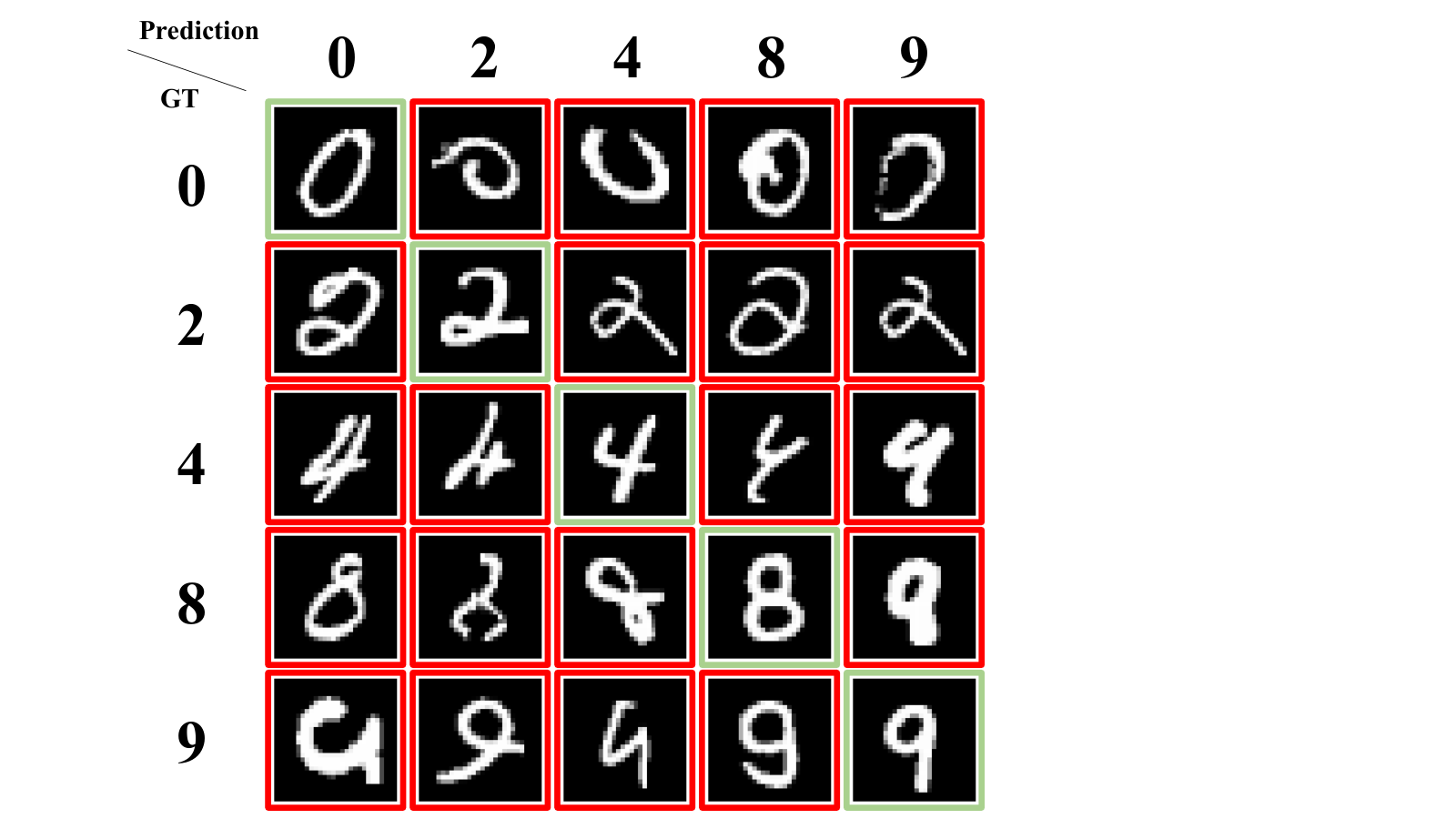
In this subsection, we pursue the excellent performance for kernel interpolation on a high-dimensional real data set MNIST, which is a hand-writing recognition application and is regarded as a benchmark of high dimensional data application. The basic experimental setting of this paper is the same as that in [21]. As shown in Figure 7, the input of the data is a hand-writing digits in {0,…,10}\{0,\dots,10\} and the prediction is also from {0,…,10}\{0,\dots,10\}. Our experiment considers the following problem: for each pair of distinct digits {(i,j)}\{(i,j)\}, i,j∈{0,1,…,9}}i,j\in\{0,1,\ldots,9\}\}, label one digit as 11 and the other as 00, then fit the kernel quasi-interpolation with Gaussian kernel Gγ​(x,x′)=exp⁡(−γ​‖x−x′‖2d)G_{\gamma}(x,x^{\prime})=\exp\left(-\frac{\gamma\|x-x^{\prime}\|^{2}}{d}\right) and γ=2​d=2×784\gamma=2d=2\times 784.

Refer to caption
Figure 7: Task of MNIST data set

For each of the C⁡(10,2)=45C(10,2)=45 pairs of experiments, we chose a finer grid of regularization λ∈[0,20],\lambda\in[0,20], where λ\lambda is the regularization parameter. We evaluate the performance on the out-of-sample test dataset, with the relative mean square error ∑i(f^​(xi)−yi)2∑i(y¯−yi)2\frac{\sum_{i}\left(\widehat{f}\left(x_{i}\right)-y_{i}\right)^{2}}{\sum_{i}\left(\bar{y}-y_{i}\right)^{2}} to measure the accuracy of interpolation. For experiment, both the training size and test size are 10,00010,000. The numerical results can be found in Figure 8.

Figure 8: Kernel interpolation on MNIST

Figure 8 (a) demonstrates the relation between the condition number of the quasi-interpolation matrix generated by (41) and the regularization λ\lambda. It is obvious that the condition number decreases with respect to λ\lambda, showing that adding the regularization term stabilizes the interpolation. However, as shown in Figure 8 (b), among all 4545 experiments, kernel interpolation without regularization (λ=0\lambda=0) remarkably performs the best. Furthermore, the above numerical results shows that the error increases with respect to λ\lambda, which implies that the regularization term plays a negative effect in kernel interpolation, neglecting its positive effect in enhancing the stability. The main reason is that for high dimensional data interpolation, the condition number, as shown in Figure 8 (a) is already very small. In this way, adding the regularization term plays an incremental role in guarantee the well-conditioness of the matrix. However, the additional regularization term inevitably degrades the approximation performance of kernel interpolation. All these show the effectiveness of kernel interpolation and the redundancy of the regularization term in tackling high dimensional data.

6 Proofs

In this section, we present the proofs of our main results.

6.1 Proofs of results stated in Section 2

The proof of Propositions 1 is somewhat standard. We present the proof for the sake of completeness.

Proof of Proposition 1.

Let SD=U​Σ​VTS_{D}=U\Sigma V^{T} be the SVD of SDS_{D}, where Σ\Sigma is a diagonal matrix, U:ℝm→ℝmU:\mathbb{R}^{m}\rightarrow\mathbb{R}^{m}, V:ℝm→ℋKV:\mathbb{R}^{m}\rightarrow\mathcal{H}_{K} satisfying UT​U=VT​V=IU^{T}U=V^{T}V=I. Then, we have

LK,D=SDT​SD=V​Σ2​VT,1m​𝕂=SD​SDT=U​Σ2​UT,L_{K,D}=S_{D}^{T}S_{D}=V\Sigma^{2}V^{T},\qquad\frac{1}{m}\mathbb{K}=S_{D}S_{D}^{T}=U\Sigma^{2}U^{T},

and

Pm:=SDT​(SD​SDT)−1​SD=V​VT.P_{m}:=S_{D}^{T}(S_{D}S_{D}^{T})^{-1}S_{D}=VV^{T}. (42)

Equation (42) implies that PmP_{m} is the projection operator from ℋK\mathcal{H}_{K} to ℋK,m=span​{ϕ1D,…,ϕmD},\mathcal{H}_{K,m}=\mbox{span}\{\phi_{1}^{D},\dots,\phi_{m}^{D}\}, which implies

Pms=Pmand​(I−Pm)s=(I−Pm),∀s∈ℤ+.P_{m}^{s}=P_{m}\qquad\mbox{and}\ (I-P_{m})^{s}=(I-P_{m}),\qquad\ \forall\ s\in\mathbb{Z}_{+}. (43)

It follows from (6) and (5) that

fD=SDT​(SD​SDT)−1​yD=SDT​(SD​SDT)−1​SD​f∗=Pm​f∗.f_{D}=S_{D}^{T}(S_{D}S_{D}^{T})^{-1}y_{D}=S_{D}^{T}(S_{D}S_{D}^{T})^{-1}S_{D}f^{*}=P_{m}f^{*}. (44)

By writing

LK,D​fD=SDT​SD​SDT​(SD​SDT)−1​SD​f∗=LK,D​f∗,L_{K,D}f_{D}=S_{D}^{T}S_{D}S_{D}^{T}(S_{D}S_{D}^{T})^{-1}S_{D}f^{*}=L_{K,D}f^{*},

This implies (7) and completes the proof of Proposition 1.

To prove Theorem 2, we need the following bounds related to the projection operator, whose proof is also given for the sake of completeness.

Proposition 14.

Let ν,λ≥0\nu,\lambda\geq 0 and j∈ℕj\in\mathbb{N}. We have

∥LKv(I−Pm)∥≤λ1/2∥LKv(LK,D+λI)−1/2∥,\|L_{K}^{v}(I-P_{m})\|\leq\lambda^{1/2}\|L_{K}^{v}(L_{K,D}+\lambda I)^{-1/2}\|, (45)

and

‖SDT​(SD​SDT)−j​SD‖≤(σmD)−j+1.\|S_{D}^{T}(S_{D}S_{D}^{T})^{-j}S_{D}\|\leq(\sigma^{D}_{m})^{-j+1}. (46)

Proof.

For arbitrary λ>0\lambda>0, since

(LK,D+λ​I)−1​SDT=(SDT​SD+λ​I)−1​SDT​(SD​SDT+λ​I)​(SD​SDT+λ​I)−1\displaystyle(L_{K,D}+\lambda I)^{-1}S_{D}^{T}=(S_{D}^{T}S_{D}+\lambda I)^{-1}S_{D}^{T}(S_{D}S_{D}^{T}+\lambda I)(S_{D}S_{D}^{T}+\lambda I)^{-1} (47)
=\displaystyle= (SDT​SD+λ​I)−1​(SDT​SD​SDT+λ​SDT)​(SD​SDT+λ​I)−1=SDT​(SD​SDT+λ​I)−1,\displaystyle(S_{D}^{T}S_{D}+\lambda I)^{-1}(S_{D}^{T}S_{D}S_{D}^{T}+\lambda S_{D}^{T})(S_{D}S_{D}^{T}+\lambda I)^{-1}=S_{D}^{T}(S_{D}S_{D}^{T}+\lambda I)^{-1},

we then have

(LK,D+λ​I)−1​LK,D\displaystyle(L_{K,D}+\lambda I)^{-1}L_{K,D} =\displaystyle= SDT​(SD​SDT+λ​I)−1​SD\displaystyle S_{D}^{T}(S_{D}S_{D}^{T}+\lambda I)^{-1}S_{D} (48)
=\displaystyle= Pm​SDT​(SD​SDT+λ​I)−1​SD​Pm.\displaystyle P_{m}S_{D}^{T}(S_{D}S_{D}^{T}+\lambda I)^{-1}S_{D}P_{m}.

It follows from (43), (48) and the inequality ‖(LK,D+λ​I)−1​LK,D‖≤1\|(L_{K,D}+\lambda I)^{-1}L_{K,D}\|\leq 1 that for any f∈ℋKf\in\mathcal{H}_{K}, there holds

⟨SDT​(SD​SDT+λ​I)−1​SD​f,f⟩K=⟨Pm​(LK,D+λ​I)−1​LK,D​Pm​f,f⟩K\displaystyle\langle S_{D}^{T}(S_{D}S_{D}^{T}+\lambda I)^{-1}S_{D}f,f\rangle_{K}=\langle P_{m}(L_{K,D}+\lambda I)^{-1}L_{K,D}P_{m}f,f\rangle_{K}
=\displaystyle= ∥(LK,D+λI)−1/2LK,D1/2Pmf∥K2≤∥(LK,D+λI)−1/2LK,D1/2∥2∥Pmf∥K2≤∥Pmf∥K2\displaystyle\|(L_{K,D}+\lambda I)^{-1/2}L_{K,D}^{1/2}P_{m}f\|_{K}^{2}\leq\|(L_{K,D}+\lambda I)^{-1/2}L_{K,D}^{1/2}\|^{2}\|P_{m}f\|_{K}^{2}\leq\|P_{m}f\|_{K}^{2}
=\displaystyle= ⟨Pm​f,f⟩K.\displaystyle\langle P_{m}f,f\rangle_{K}.

This shows that Pm−(LK,D+λ​I)−1​LK,DP_{m}-(L_{K,D}+\lambda I)^{-1}L_{K,D} is a positive operator. We then obtain from λ​(LK,D+λ​I)−1=I−(LK,D+λ​I)−1​LK,D\lambda(L_{K,D}+\lambda I)^{-1}=I-(L_{K,D}+\lambda I)^{-1}L_{K,D} that λ​(LK,D+λ​I)−1−(I−Pm)\lambda(L_{K,D}+\lambda I)^{-1}-(I-P_{m}) is positive, which in turns implies that LKv​(λ​(LK,D+λ​I)−1−(I−Pm))​LKvL_{K}^{v}(\lambda(L_{K,D}+\lambda I)^{-1}-(I-P_{m}))L_{K}^{v} is positive. Recalling (43), we have

λ∥(LK,D+λI)−1/2LKvf∥K2=⟨λ(LK,D+λI)−1LKvf,LKvf⟩K\displaystyle\lambda\|(L_{K,D}+\lambda I)^{-1/2}L_{K}^{v}f\|_{K}^{2}=\langle\lambda(L_{K,D}+\lambda I)^{-1}L_{K}^{v}f,L_{K}^{v}f\rangle_{K}
=\displaystyle= ⟨LKv​λ​(LK,D+λ​I)−1​LKv​f,f⟩K≥⟨LKv​(I−Pm)​LKv​f,f⟩K=⟨LKv​(I−Pm)2​LKv​f,f⟩K\displaystyle\langle L_{K}^{v}\lambda(L_{K,D}+\lambda I)^{-1}L_{K}^{v}f,f\rangle_{K}\geq\langle L_{K}^{v}(I-P_{m})L_{K}^{v}f,f\rangle_{K}=\langle L_{K}^{v}(I-P_{m})^{2}L_{K}^{v}f,f\rangle_{K}
=\displaystyle= ⟨(I−Pm)​LKv​f,(I−Pm)​LKv​f⟩K=‖LKv​(I−Pm)​f‖K\displaystyle\langle(I-P_{m})L_{K}^{v}f,(I-P_{m})L_{K}^{v}f\rangle_{K}=\|L_{K}^{v}(I-P_{m})f\|_{K}

holds true for any f∈ℋKf\in\mathcal{H}_{K} and any v≥0v\geq 0, which proves (45). Since SDT​(SD​SDT)−j​SDS_{D}^{T}(S_{D}S_{D}^{T})^{-j}S_{D} is self-adjoint, direct computation yields

(SDT​(SD​SDT)−j​SD)k=SDT​(SD​SDT)−j​k+k−1​SD,∀k∈ℕ.(S_{D}^{T}(S_{D}S_{D}^{T})^{-j}S_{D})^{k}=S_{D}^{T}(S_{D}S_{D}^{T})^{-jk+k-1}S_{D},\qquad\forall\ k\in\mathbb{N}.

This implies that

‖SDT​(SD​SDT)−j​SD‖k=‖(SDT​(SD​SDT)−j​SD)k‖=‖SDT​(SD​SDT)−j​k+k−1​SD‖.\|S_{D}^{T}(S_{D}S_{D}^{T})^{-j}S_{D}\|^{k}=\|(S_{D}^{T}(S_{D}S_{D}^{T})^{-j}S_{D})^{k}\|=\|S_{D}^{T}(S_{D}S_{D}^{T})^{-jk+k-1}S_{D}\|. (49)

Note that for any 𝐜=(c1,…,cm)T∈ℝm{\bf c}=(c_{1},\dots,c_{m})^{T}\in\mathbb{R}^{m}, there holds

‖SDT​𝐜‖K2=1m2​∑i=1m∑j=1mci​cj​⟨Kxi,Kxj⟩K≤κ2​(1m​∑i=1m|ci|)2≤κ2m​∑i=1m|ci|2=κ2m​‖𝐜‖ℓ22.\|S_{D}^{T}{\bf c}\|_{K}^{2}=\frac{1}{m^{2}}\sum_{i=1}^{m}\sum_{j=1}^{m}c_{i}c_{j}\langle K_{x_{i}},K_{x_{j}}\rangle_{K}\leq\kappa^{2}\left(\frac{1}{m}\sum_{i=1}^{m}|c_{i}|\right)^{2}\leq\frac{\kappa^{2}}{m}\sum_{i=1}^{m}|c_{i}|^{2}=\frac{\kappa^{2}}{m}\|{\bf c}\|_{\ell^{2}}^{2}.

The compactness of 𝒳\mathcal{X} implies κ<∞\kappa<\infty. This allows us to use the fact that ‖f‖∞≤κ​‖f‖K\|f\|_{\infty}\leq\kappa\|f\|_{K} for f∈ℋKf\in\mathcal{H}_{K} to deduce

‖SDT​(SD​SDT)−j​k+k−1​SD​f‖K2≤κ2m​‖(SD​SDT)−j​k+k−1​SD​f‖ℓ22\displaystyle\|S_{D}^{T}(S_{D}S_{D}^{T})^{-jk+k-1}S_{D}f\|^{2}_{K}\leq\frac{\kappa^{2}}{m}\|(S_{D}S_{D}^{T})^{-jk+k-1}S_{D}f\|_{\ell^{2}}^{2}
≤\displaystyle\leq κ2m​(σmD)−2​j​k+2​k−2​‖SD​f‖ℓ22≤κ2​(σmD)−2​j​k+2​k−2​1m​∑i=1m|f⁡(xi)|2\displaystyle\frac{\kappa^{2}}{m}\left(\sigma^{D}_{m}\right)^{-2jk+2k-2}\|S_{D}f\|_{\ell^{2}}^{2}\leq\kappa^{2}\left(\sigma^{D}_{m}\right)^{-2jk+2k-2}\frac{1}{m}\sum_{i=1}^{m}|f(x_{i})|^{2}
≤\displaystyle\leq κ2​(σmD)−2​j​k+2​k−2​‖f‖∞2≤κ4​(σmD)−2​j​k+2​k−2​‖f‖K2.\displaystyle\kappa^{2}\left(\sigma^{D}_{m}\right)^{-2jk+2k-2}\|f\|_{\infty}^{2}\leq\kappa^{4}\left(\sigma^{D}_{m}\right)^{-2jk+2k-2}\|f\|_{K}^{2}.

Hence,

‖SDT​(SD​SDT)−j​SD‖≤κ2/k​(σmD)−j+1−1/k.\|S_{D}^{T}(S_{D}S_{D}^{T})^{-j}S_{D}\|\leq{\kappa^{2/k}}\left(\sigma^{D}_{m}\right)^{-j+1-1/k}.

Note that the above estimate holds true all k∈ℕk\in\mathbb{N}. Letting k→∞k\rightarrow\infty, we derive

‖SDT​(SD​SDT)−j​SD‖≤(σmD)−j+1.\|S_{D}^{T}(S_{D}S_{D}^{T})^{-j}S_{D}\|\leq(\sigma^{D}_{m})^{-j+1}.

This completes the proof of Proposition 14.

With the help of the above proposition, we can prove Theorem 2 as follows.

Proof of Theorem 2.

Assuming (9) with r≥1/2r\geq 1/2, we use the facts that ‖A​f‖≤‖A‖​‖f‖K\|Af\|\leq\|A\|\|f\|_{K}, ‖A​B‖=‖B​A‖≤‖A‖​‖B‖\|AB\|=\|BA\|\leq\|A\|\|B\| for positive operators A,BA,B and f∈ℋKf\in\mathcal{H}_{K} to derive

‖LKu​(fD−f∗)‖ρ=‖LKu​(I−Pm)​LKr−1/2​ℒK1/2​h∗‖K≤‖LKu​(I−Pm)​LKr−1/2‖​‖h∗‖ρ.\|L_{K}^{u}(f_{D}-f^{*})\|_{\rho}=\|L_{K}^{u}(I-P_{m})L_{K}^{r-1/2}\mathcal{L}_{K}^{1/2}h^{*}\|_{K}\leq\|L_{K}^{u}(I-P_{m})L_{K}^{r-1/2}\|\|h^{*}\|_{\rho}. (50)

In the rest of the proof, we need to work on two cases: r>1r>1 and 12≤r≤1\frac{1}{2}\leq r\leq 1.

(i) Case: 12≤r≤1\frac{1}{2}\leq r\leq 1. We first use (43) to derive that (I−Pm)2​r=(I−Pm)(I-P_{m})^{2r}=(I-P_{m}). We then use (45) with v=1/2v=1/2 and the well-known Codes inequality (63) (in Appendix A) with τ=2​u\tau=2u and τ=2​r−1\tau=2r-1 respectively to get

‖LKu​(I−Pm)​LKr−1/2‖=‖LKu​(I−Pm)2​r−1+2​u​LKr−1/2‖\displaystyle\|L_{K}^{u}(I-P_{m})L_{K}^{r-1/2}\|=\|L_{K}^{u}(I-P_{m})^{2r-1+2u}L_{K}^{r-1/2}\|
≤\displaystyle\leq ‖LKu​(I−Pm)2​u‖​‖(I−Pm)2​r−1​LKr−1/2‖≤‖LK1/2​(I−Pm)‖2​u​‖(I−Pm)​LK1/2‖2​r−1\displaystyle\|L_{K}^{u}(I-P_{m})^{2u}\|\|(I-P_{m})^{2r-1}L_{K}^{r-1/2}\|\leq\|L_{K}^{1/2}(I-P_{m})\|^{2u}\|(I-P_{m})L_{K}^{1/2}\|^{2r-1}
=\displaystyle= ∥(I−Pm)LK1/2∥2​r+2​u−1≤λr+u−1/2∥(LK,D+λI)−1/2(LK+λI)1/2∥2​r+2​u−1.\displaystyle\|(I-P_{m})L_{K}^{1/2}\|^{2r+2u-1}\leq\lambda^{r+u-1/2}\|(L_{K,D}+\lambda I)^{-1/2}(L_{K}+\lambda I)^{1/2}\|^{2r+2u-1}.

Plugging the above estimate into (50) and noting (11), we have

‖LKu​(fD−f∗)‖ρ≤λr+u−1/2​𝒬D,λ2​r+2​u−1​‖h∗‖ρ.\|L_{K}^{u}(f_{D}-f^{*})\|_{\rho}\leq\lambda^{r+u-1/2}\mathcal{Q}_{D,\lambda}^{2r+2u-1}\|h^{*}\|_{\rho}.

(ii)Case: r>1r>1. We first use the triangle inequality to get

‖LKu​(I−Pm)​LKr−1/2‖≤‖LKu​(I−Pm)​(LKr−1/2−LK,Dr−1/2)‖+‖LKu​(I−Pm)​LK,Dr−1/2‖.\displaystyle\|L_{K}^{u}(I-P_{m})L_{K}^{r-1/2}\|\leq\|L_{K}^{u}(I-P_{m})(L_{K}^{r-1/2}-L_{K,D}^{r-1/2})\|+\|L_{K}^{u}(I-P_{m})L_{K,D}^{r-1/2}\|.

Since r>1r>1, we have r−1/2>1/2r-1/2>1/2. Thus (7) implies

‖LKu​(I−Pm)​LK,Dr−1/2‖≤‖LKu‖​‖LK,Dr−1/2​(I−Pm)‖=0.\|L_{K}^{u}(I-P_{m})L_{K,D}^{r-1/2}\|\leq\|L_{K}^{u}\|\|L_{K,D}^{r-1/2}(I-P_{m})\|=0.

Hence, (45) with v=1/2v=1/2 and (64) in Appendix A yield

‖LKu​(I−Pm)​LKr−1/2‖≤‖LKu​(I−Pm)​(LKr−1/2−LK,Dr−1/2)‖\displaystyle\|L_{K}^{u}(I-P_{m})L_{K}^{r-1/2}\|\leq\|L_{K}^{u}(I-P_{m})(L_{K}^{r-1/2}-L_{K,D}^{r-1/2})\|
≤\displaystyle\leq ‖LKu​(I−Pm)‖​‖LKr−1/2−LK,Dr−1/2‖≤‖LKu​(I−Pm)2​u‖​‖LKr−1/2−LK,Dr−1/2‖H​S\displaystyle\|L_{K}^{u}(I-P_{m})\|\|L_{K}^{r-1/2}-L_{K,D}^{r-1/2}\|\leq\|L_{K}^{u}(I-P_{m})^{2u}\|\|L_{K}^{r-1/2}-L_{K,D}^{r-1/2}\|_{HS}
≤\displaystyle\leq (r−1/2)κr−3/2λu∥(LK,D+λI)−1/2(LK+λI)1/2∥∥LK−LK,D∥H​S.\displaystyle(r-1/2)\kappa^{r-3/2}\lambda^{u}\|(L_{K,D}+\lambda I)^{-1/2}(L_{K}+\lambda I)^{1/2}\|\|L_{K}-L_{K,D}\|_{HS}.

Inserting the above estimate into (50) and noting (11), (12), we obtain

‖LKu​(fD−f∗)‖K≤(r−1/2)​κr−3/2​‖h∗‖ρ​λu​𝒬D,λ​ℛD.\|L_{K}^{u}(f_{D}-f^{*})\|_{K}\leq(r-1/2)\kappa^{r-3/2}\|h^{*}\|_{\rho}\lambda^{u}\mathcal{Q}_{D,\lambda}\mathcal{R}_{D}.

This completes the proof of Theorem 2.

The proof of Theorem 5 requires a novel integral operator approach as well as a second-order decomposition of difference of operators developed in [22, 11]. We proceed it as follows.

Proof of Theorem 5.

Define fD∗=Pm​f∗f_{D}^{*}=P_{m}f^{*}. We then write,

‖LKu​(fD−f∗)‖K≤‖LKu​(fD−fD∗)‖K+‖LKu​(fD∗−f∗)‖K.\|L_{K}^{u}(f_{D}-f^{*})\|_{K}\leq\|L_{K}^{u}(f_{D}-f_{D}^{*})\|_{K}+\|L_{K}^{u}(f_{D}^{*}-f^{*})\|_{K}. (51)

The term ‖LKu​(fD∗−f∗)‖K\|L_{K}^{u}(f_{D}^{*}-f^{*})\|_{K} has been dealt with in the proof of Theorem 2, which allows us to concentrate on bounding ‖LKu​(fD−fD∗)‖K\|L_{K}^{u}(f_{D}-f_{D}^{*})\|_{K}. The crux of our proof is to introduce the following second-order decomposition for differences of operators. A prototype of this decomposition can be found in [22, 11]. Let A,BA,B be invertible operators. We first write

A−1−B−1=A−1​(B−A)​B−1=B−1​(B−A)​A−1.A^{-1}-B^{-1}=A^{-1}(B-A)B^{-1}=B^{-1}(B-A)A^{-1}. (52)

We then use (52) to write

A−1−B−1=B−1​(B−A)​B−1+B−1​(B−A)​A−1​(B−A)​B−1.A^{-1}-B^{-1}=B^{-1}(B-A)B^{-1}+B^{-1}(B-A)A^{-1}(B-A)B^{-1}. (53)

Setting A=SD​SDTA=S_{D}S_{D}^{T} and B=SD​SDT+μ​IB=S_{D}S_{D}^{T}+\mu I with μ>0\mu>0 in (53), we obtain that

(SD​SDT)−1\displaystyle(S_{D}S_{D}^{T})^{-1} =\displaystyle= (SD​SDT+μ​I)−1+μ​(SD​SDT+μ​I)−2\displaystyle(S_{D}S_{D}^{T}+\mu I)^{-1}+\mu(S_{D}S_{D}^{T}+\mu I)^{-2}
+\displaystyle+ μ2​(SD​SDT+μ​I)−1​(SD​SDT)−1​(SD​SDT+μ​I)−1.\displaystyle\mu^{2}(S_{D}S_{D}^{T}+\mu I)^{-1}(S_{D}S_{D}^{T})^{-1}(S_{D}S_{D}^{T}+\mu I)^{-1}.

Note that (47) implies

SDT​(SD​SDT+μ​I)−k=(LK,D+μ​I)−k​SDT,∀k∈ℕ.S^{T}_{D}(S_{D}S_{D}^{T}+\mu I)^{-k}=(L_{K,D}+\mu I)^{-k}S_{D}^{T},\qquad\forall\ k\in\mathbb{N}. (54)

Hence, we have

SDT​(SD​SDT)−1​(yD−SD​f∗)=SDT​(SD​SDT+μ​I)−1​(yD−SD​f∗)\displaystyle S_{D}^{T}(S_{D}S_{D}^{T})^{-1}(y_{D}-S_{D}f^{*})=S_{D}^{T}(S_{D}S_{D}^{T}+\mu I)^{-1}(y_{D}-S_{D}f^{*})
+\displaystyle+ μ​SDT​(SD​SDT+μ​I)−2​(yD−SD​f∗)\displaystyle\mu S_{D}^{T}(S_{D}S_{D}^{T}+\mu I)^{-2}(y_{D}-S_{D}f^{*})
+\displaystyle+ μ2​SDT​(SD​SDT+μ​I)−1​(SD​SDT)−1​(SD​SDT+μ​I)−1​(yD−SD​f∗)\displaystyle\mu^{2}S_{D}^{T}(S_{D}S_{D}^{T}+\mu I)^{-1}(S_{D}S_{D}^{T})^{-1}(S_{D}S_{D}^{T}+\mu I)^{-1}(y_{D}-S_{D}f^{*})
=\displaystyle= (LK,D+μ​I)−1​(SDT​yD−LK,D​f∗)+μ​(LK,D+μ​I)−2​(SDT​yD−LK,D​f∗)\displaystyle(L_{K,D}+\mu I)^{-1}(S_{D}^{T}y_{D}-L_{K,D}f^{*})+\mu(L_{K,D}+\mu I)^{-2}(S_{D}^{T}y_{D}-L_{K,D}f^{*})
+\displaystyle+ μ2​(LK,D+μ​I)−1​SDT​(SD​SDT)−2​SD​(LK,D+μ​I)−1​(SDT​yD−LK,D​f∗).\displaystyle\mu^{2}(L_{K,D}+\mu I)^{-1}S_{D}^{T}(S_{D}S_{D}^{T})^{-2}S_{D}(L_{K,D}+\mu I)^{-1}(S_{D}^{T}y_{D}-L_{K,D}f^{*}).

Therefore, it follows from (15) and (11) that

‖LKu​(fD−fD∗)‖K=‖LKu​SDT​(SD​SDT)−1​(yD−SD​f∗)‖K\displaystyle\|L_{K}^{u}(f_{D}-f^{*}_{D})\|_{K}=\|L_{K}^{u}S_{D}^{T}(S_{D}S_{D}^{T})^{-1}(y_{D}-S_{D}f^{*})\|_{K}
≤\displaystyle\leq ‖LKu​(LK,D+μ​I)−1​(SDT​yD−LK,D​f∗)‖K+μ​‖LKu​(LK,D+μ​I)−2​(SDT​yD−LK,D​f∗)‖K\displaystyle\|L_{K}^{u}(L_{K,D}+\mu I)^{-1}(S_{D}^{T}y_{D}-L_{K,D}f^{*})\|_{K}+\mu\|L_{K}^{u}(L_{K,D}+\mu I)^{-2}(S_{D}^{T}y_{D}-L_{K,D}f^{*})\|_{K}
+\displaystyle+ μ2​‖LKu​(LK,D+μ​I)−1​SDT​(SD​SDT)−2​SD​(LK,D+μ​I)−1​(SDT​yD−LK,D​f∗)‖K\displaystyle\mu^{2}\|L_{K}^{u}(L_{K,D}+\mu I)^{-1}S_{D}^{T}(S_{D}S_{D}^{T})^{-2}S_{D}(L_{K,D}+\mu I)^{-1}(S_{D}^{T}y_{D}-L_{K,D}f^{*})\|_{K}
≤\displaystyle\leq 2​μu−1/2​𝒬D,μ2​𝒫D,μ+μu+1/2​𝒬D,μ2​u+1​𝒫D,μ​‖SDT​(SD​SDT)−2​SD‖.\displaystyle 2\mu^{u-1/2}\mathcal{Q}^{2}_{D,\mu}\mathcal{P}_{D,\mu}+\mu^{u+1/2}\mathcal{Q}^{2u+1}_{D,\mu}\mathcal{P}_{D,\mu}\|S_{D}^{T}(S_{D}S_{D}^{T})^{-2}S_{D}\|.

Applying inequality (46) with j=2j=2, we have

‖LKu​(fD−fD∗)‖K≤(2​μu−1/2+μu+1/2​(σmD)−1​𝒬D,μ2​u−1)​𝒬D,μ2​𝒫D,μ,∀μ>0.\|L_{K}^{u}(f_{D}-f^{*}_{D})\|_{K}\leq(2\mu^{u-1/2}+{\mu^{u+1/2}}(\sigma^{D}_{m})^{-1}\mathcal{Q}^{2u-1}_{D,\mu})\mathcal{Q}^{2}_{D,\mu}\mathcal{P}_{D,\mu},\qquad\forall\ \mu>0.

Inserting the above estimate into (51) and noting (13), we derive (5) directly. This completes the proof of Theorem 5.

The main difficulty in the proof of Theorem 7 is to find a good projection of f∗f^{*} onto ℋK\mathcal{H}_{K} and quantify the error. In our proof, we construct a fλ∈ℋKf_{\lambda}\in\mathcal{H}_{K} and treat f∗−fλf^{*}-f_{\lambda} as the noise. In such a way, the basic idea is similar as that in the proof of Theorem 5 by involving σmD\sigma_{m}^{D} to reflect the stability of kernel interpolation.

Proof of Theorem 7.

For an arbitrary λ>0\lambda>0, define

fλ=(LK+λ​I)−1​ℒK​f∗,fD,λ=(LK,D+λ​I)−1​ℒK,D​f∗.f_{\lambda}=(L_{K}+\lambda I)^{-1}\mathcal{L}_{K}f^{*},\qquad f_{D,\lambda}=(L_{K,D}+\lambda I)^{-1}\mathcal{L}_{K,D}f^{*}.

Assuming that (9) holds true with 0≤r≤10\leq r\leq 1, Smale and Zhou [40] (or [41]) proved that

‖f∗−fλ‖ρ≤λr​‖h∗‖ρ.\|f^{*}-f_{\lambda}\|_{\rho}\leq\lambda^{r}\|h^{*}\|_{\rho}. (55)

Thus, we have

‖f∗−fD‖ρ≤λr​‖h∗‖ρ+‖fλ−fD,λ‖ρ+‖fD,λ−fD‖ρ.\|f^{*}-f_{D}\|_{\rho}\leq\lambda^{r}\|h^{*}\|_{\rho}+\|f_{\lambda}-f_{D,\lambda}\|_{\rho}+\|f_{D,\lambda}-f_{D}\|_{\rho}. (56)

By writing

fλ−fD,λ=(LK+λ​I)−1​ℒK​f∗−(LK,D+λ​I)−1​ℒK,D​f∗\displaystyle f_{\lambda}-f_{D,\lambda}=(L_{K}+\lambda I)^{-1}\mathcal{L}_{K}f^{*}-(L_{K,D}+\lambda I)^{-1}\mathcal{L}_{K,D}f^{*}
=\displaystyle= [(LK+λ​I)−1−(LK,D+λ​I)−1]​ℒK​f∗+(LK,D+λ​I)−1​(ℒK,D​f∗−ℒK​f∗)\displaystyle[(L_{K}+\lambda I)^{-1}-(L_{K,D}+\lambda I)^{-1}]\mathcal{L}_{K}f^{*}+(L_{K,D}+\lambda I)^{-1}(\mathcal{L}_{K,D}f^{*}-\mathcal{L}_{K}f^{*})
=\displaystyle= (LK,D+λ​I)−1​(LK,D−LK)​(LK+λ​I)−1​ℒK​f∗+(LK,D+λ​I)−1​(ℒK,D​f∗−ℒK​f∗).\displaystyle(L_{K,D}+\lambda I)^{-1}(L_{K,D}-L_{K})(L_{K}+\lambda I)^{-1}\mathcal{L}_{K}f^{*}+(L_{K,D}+\lambda I)^{-1}(\mathcal{L}_{K,D}f^{*}-\mathcal{L}_{K}f^{*}).

we obtain

‖fλ−fD,λ‖ρ\displaystyle\|f_{\lambda}-f_{D,\lambda}\|_{\rho} ≤\displaystyle\leq ‖LK1/2​(LK,D+λ​I)−1​(LK,D−LK)​(LK+λ​I)−1​LK1/2+r​ℒK1/2​h∗‖K\displaystyle\|L_{K}^{1/2}(L_{K,D}+\lambda I)^{-1}(L_{K,D}-L_{K})(L_{K}+\lambda I)^{-1}L_{K}^{1/2+r}\mathcal{L}_{K}^{1/2}h^{*}\|_{K} (57)
+\displaystyle+ ‖LK1/2​(LK,D+λ​I)−1​(ℒK,D​f∗−ℒK​f∗)‖K\displaystyle\|L_{K}^{1/2}(L_{K,D}+\lambda I)^{-1}(\mathcal{L}_{K,D}f^{*}-\mathcal{L}_{K}f^{*})\|_{K}
≤\displaystyle\leq λr−1/2​𝒬D,λ2​𝒲D,λ​‖h∗‖ρ+𝒬D,λ2​𝒰D,λ,f∗.\displaystyle\lambda^{r-1/2}\mathcal{Q}_{D,\lambda}^{2}\mathcal{W}_{D,\lambda}\|h^{*}\|_{\rho}+\mathcal{Q}^{2}_{D,\lambda}\mathcal{U}_{D,\lambda,f^{*}}.

It follows from (53) with A=SD​SDTA=S_{D}S_{D}^{T} and B=SD​SDT+λ​IB=S_{D}S_{D}^{T}+\lambda I and (54) that

fD−fD,λ=SDT​((SD​SDT)−1−(SD​SDT+λ)−1)​𝒮D​f∗\displaystyle f_{D}-f_{D,\lambda}=S_{D}^{T}((S_{D}S_{D}^{T})^{-1}-(S_{D}S_{D}^{T}+\lambda)^{-1})\mathcal{S}_{D}f^{*}
=\displaystyle= λ​SDT​(SD​SDT+λ​I)−2​𝒮D​f∗+λ2​SDT​(SD​SDT+λ​I)−1​(SD​SDT)−1​(SD​SDT+λ​I)−1​𝒮D​f∗\displaystyle\lambda S_{D}^{T}(S_{D}S_{D}^{T}+\lambda I)^{-2}\mathcal{S}_{D}f^{*}+\lambda^{2}S_{D}^{T}(S_{D}S_{D}^{T}+\lambda I)^{-1}(S_{D}S_{D}^{T})^{-1}(S_{D}S_{D}^{T}+\lambda I)^{-1}\mathcal{S}_{D}f^{*}
=\displaystyle= λ​(LK,D+λ​I)−2​ℒK,D​f∗+λ2​(LK,D+λ​I)−1​SDT​(SD​SDT)−2​SD​(LK,D+λ​I)−1​ℒK,D​f∗\displaystyle\lambda(L_{K,D}+\lambda I)^{-2}\mathcal{L}_{K,D}f^{*}+\lambda^{2}(L_{K,D}+\lambda I)^{-1}S_{D}^{T}(S_{D}S_{D}^{T})^{-2}S_{D}(L_{K,D}+\lambda I)^{-1}\mathcal{L}_{K,D}f^{*}
=\displaystyle= λ​(LK,D+λ​I)−2​(ℒK,D−ℒK)​f∗+λ​(LK,D+λ​I)−2​ℒK​f∗\displaystyle\lambda(L_{K,D}+\lambda I)^{-2}(\mathcal{L}_{K,D}-\mathcal{L}_{K})f^{*}+\lambda(L_{K,D}+\lambda I)^{-2}\mathcal{L}_{K}f^{*}
+\displaystyle+ λ2​(LK,D+λ​I)−1​SDT​(SD​SDT)−2​SD​(LK,D+λ​I)−1​(ℒK,D−ℒK)​f∗\displaystyle\lambda^{2}(L_{K,D}+\lambda I)^{-1}S_{D}^{T}(S_{D}S_{D}^{T})^{-2}S_{D}(L_{K,D}+\lambda I)^{-1}(\mathcal{L}_{K,D}-\mathcal{L}_{K})f^{*}
+\displaystyle+ λ2​(LK,D+λ​I)−1​SDT​(SD​SDT)−2​SD​(LK,D+λ​I)−1​ℒK​f∗.\displaystyle\lambda^{2}(L_{K,D}+\lambda I)^{-1}S_{D}^{T}(S_{D}S_{D}^{T})^{-2}S_{D}(L_{K,D}+\lambda I)^{-1}\mathcal{L}_{K}f^{*}.

Using (11), (21), and (63) (Appendix A), and the fact that ‖A​f‖K≤‖A‖​‖f‖K\|Af\|_{K}\leq\|A\|\|f\|_{K} for positive operator AA and f∈ℋKf\in\mathcal{H}_{K}, we derive

‖λ​(LK,D+λ​I)−2​(ℒK,D−ℒK)​f∗‖ρ=λ​‖LK1/2​(LK,D+λ​I)−2​(ℒK,D−ℒK)​f∗‖K\displaystyle\|\lambda(L_{K,D}+\lambda I)^{-2}(\mathcal{L}_{K,D}-\mathcal{L}_{K})f^{*}\|_{\rho}=\lambda\|L_{K}^{1/2}(L_{K,D}+\lambda I)^{-2}(\mathcal{L}_{K,D}-\mathcal{L}_{K})f^{*}\|_{K}
≤\displaystyle\leq λ​𝒬D,λ​λ−1​𝒬D,λ​𝒰D,λ,f∗=𝒬D,λ2​𝒰D,λ,f∗,\displaystyle\lambda\mathcal{Q}_{D,\lambda}\lambda^{-1}\mathcal{Q}_{D,\lambda}\mathcal{U}_{D,\lambda,f^{*}}=\mathcal{Q}_{D,\lambda}^{2}\mathcal{U}_{D,\lambda,f^{*}},
‖λ​(LK,D+λ​I)−2​ℒK​f∗‖ρ≤λ​‖LK1/2​(LK,D+λ​I)−2​LK1/2+r‖​‖ℒK1/2​h∗‖K\displaystyle\|\lambda(L_{K,D}+\lambda I)^{-2}\mathcal{L}_{K}f^{*}\|_{\rho}\leq\lambda\|L_{K}^{1/2}(L_{K,D}+\lambda I)^{-2}L_{K}^{1/2+r}\|\|\mathcal{L}_{K}^{1/2}h^{*}\|_{K}
≤\displaystyle\leq λ​𝒬D,λ​λ−2+1+r​𝒬D,λ2​r+1​‖h∗‖ρ=‖h∗‖ρ​λr​𝒬D,λ2​r+2.\displaystyle\lambda\mathcal{Q}_{D,\lambda}\lambda^{-2+1+r}\mathcal{Q}_{D,\lambda}^{2r+1}\|h^{*}\|_{\rho}=\|h^{*}\|_{\rho}\lambda^{r}\mathcal{Q}_{D,\lambda}^{2r+2}.

Incorporating (46), we further derive that

‖λ2​(LK,D+λ​I)−1​SDT​(SD​SDT)−2​SD​(LK,D+λ​I)−1​(ℒK,D−ℒK)​f∗‖ρ\displaystyle\|\lambda^{2}(L_{K,D}+\lambda I)^{-1}S_{D}^{T}(S_{D}S_{D}^{T})^{-2}S_{D}(L_{K,D}+\lambda I)^{-1}(\mathcal{L}_{K,D}-\mathcal{L}_{K})f^{*}\|_{\rho}
≤\displaystyle\leq λ2​‖LK1/2​(LK,D+λ​I)−1​‖‖SDT​(SD​SDT)−2​SD‖‖​(LK,D+λ​I)−1​(ℒK,D−ℒK)​f∗‖K\displaystyle\lambda^{2}\|L_{K}^{1/2}(L_{K,D}+\lambda I)^{-1}\|\|S_{D}^{T}(S_{D}S_{D}^{T})^{-2}S_{D}\|\|(L_{K,D}+\lambda I)^{-1}(\mathcal{L}_{K,D}-\mathcal{L}_{K})f^{*}\|_{K}
≤\displaystyle\leq λ2𝒬D,λλ−1/2(σmD)−1λ−1/2𝒬D,λ𝒰D,λ,f∗=λ(σmD)−1𝒬D,λ2𝒰D,λ,f∗,\displaystyle\lambda^{2}\mathcal{Q}_{D,\lambda}\lambda^{-1/2}(\sigma_{m}^{D})^{-1}\lambda^{-1/2}\mathcal{Q}_{D,\lambda}\mathcal{U}_{D,\lambda,f^{*}}=\lambda(\sigma_{m}^{D})^{-1}\mathcal{Q}^{2}_{D,\lambda}\mathcal{U}_{D,\lambda,f^{*}},
‖λ2​(LK,D+λ​I)−1​SDT​(SD​SDT)−2​SD​(LK,D+λ​I)−1​ℒK​f∗‖ρ\displaystyle\|\lambda^{2}(L_{K,D}+\lambda I)^{-1}S_{D}^{T}(S_{D}S_{D}^{T})^{-2}S_{D}(L_{K,D}+\lambda I)^{-1}\mathcal{L}_{K}f^{*}\|_{\rho}
≤\displaystyle\leq λ2​‖LK1/2​(LK,D+λ​I)−1‖|SDT​(SD​SDT)−2​SD​‖(LK,D+λ​I)−1​LK1/2+r‖​‖ℒ1/2​h∗‖K\displaystyle\lambda^{2}\|L_{K}^{1/2}(L_{K,D}+\lambda I)^{-1}\|\|S_{D}^{T}(S_{D}S_{D}^{T})^{-2}S_{D}\|(L_{K,D}+\lambda I)^{-1}L_{K}^{1/2+r}\|\|\mathcal{L}^{1/2}h^{*}\|_{K}
≤\displaystyle\leq λ2𝒬D,λλ−1/2(σmD)−1λ−1/2+r𝒬D,λ2​r+1∥h∗∥ρ=λ1+r(σmD)−1𝒬D,λ2​r+2∥h∗∥ρ.\displaystyle\lambda^{2}\mathcal{Q}_{D,\lambda}\lambda^{-1/2}(\sigma_{m}^{D})^{-1}\lambda^{-1/2+r}\mathcal{Q}_{D,\lambda}^{2r+1}\|h^{*}\|_{\rho}=\lambda^{1+r}(\sigma_{m}^{D})^{-1}\mathcal{Q}_{D,\lambda}^{2r+2}\|h^{*}\|_{\rho}.

It therefore follows that

‖fD−fD,λ‖ρ≤(1+λ​(σmD)−1)​(𝒬D,λ2​𝒰D,λ,f∗+‖h∗‖ρ​λr​𝒬D,λ2​r+2).\|f_{D}-f_{D,\lambda}\|_{\rho}\leq(1+\lambda(\sigma_{m}^{D})^{-1})(\mathcal{Q}_{D,\lambda}^{2}\mathcal{U}_{D,\lambda,f^{*}}+\|h^{*}\|_{\rho}\lambda^{r}\mathcal{Q}_{D,\lambda}^{2r+2}). (58)

Plugging (55) and (57) into (58), we have

‖f∗−fD‖ρ≤λr​‖h∗‖ρ+λr−1/2​𝒬D,λ2​𝒲D,λ​‖h∗‖ρ+𝒬D,λ​𝒰D,λ,f∗\displaystyle\|f^{*}-f_{D}\|_{\rho}\leq\lambda^{r}\|h^{*}\|_{\rho}+\lambda^{r-1/2}\mathcal{Q}_{D,\lambda}^{2}\mathcal{W}_{D,\lambda}\|h^{*}\|_{\rho}+\mathcal{Q}_{D,\lambda}\mathcal{U}_{D,\lambda,f^{*}}
+\displaystyle+ (1+λ​(σmD)−1)​(𝒬D,λ2​𝒰D,λ,f∗2+‖h∗‖ρ​λr​𝒬D,λ2​r+2),\displaystyle(1+\lambda(\sigma_{m}^{D})^{-1})(\mathcal{Q}_{D,\lambda}^{2}\mathcal{U}^{2}_{D,\lambda,f^{*}}+\|h^{*}\|_{\rho}\lambda^{r}\mathcal{Q}_{D,\lambda}^{2r+2}),

which is the desired result.

6.2 Proofs of results stated in Section 3

In this part, we aim to prove results in Section 4. The main tools in our analysis are tight bounds for operator differences presented in Appendix B. Combine Theorem 2 with Appendix B, we can prove Theorem 10 as follows.

Proof of Theorem 8.

If 12≤r≤1\frac{1}{2}\leq r\leq 1, we get from Lemma 21 in Appendix B that with confidence 1−δ1-\delta, there holds

𝒬D,λ2​r≤2r​(2​κ​(κ+8)​𝒜D,λ+1)2​r​log4​r​8δ.\displaystyle\mathcal{Q}_{D,\lambda}^{2r}\leq 2^{r}\left(2\kappa(\kappa+8)\mathcal{A}_{D,\lambda}+1\right)^{2r}\log^{4r}\frac{8}{\delta}.

Then, it follows from Theorem 2 with u=1/2u=1/2 that with confidence 1−δ1-\delta, there holds

‖fD−f∗‖ρ≤minλ>0⁡2r​‖h∗‖ρ​λr​(2​κ​(κ+8)​𝒜D,λ+1)2​r​log4​r​8δ.\|f_{D}-f^{*}\|_{\rho}\leq\min_{\lambda>0}2^{r}\|h^{*}\|_{\rho}\lambda^{r}\left(2\kappa(\kappa+8)\mathcal{A}_{D,\lambda}+1\right)^{2r}\log^{4r}\frac{8}{\delta}.

If r>1r>1, then Lemma 15 and Lemma 21 in Appendix B show that with confidence 1−δ1-\delta, there holds

𝒬D,λ​ℛD≤2​2​κ2m​(2​κ​(κ+8)​𝒜D,λ+1)​log3​16δ.\mathcal{Q}_{D,\lambda}\mathcal{R}_{D}\leq\frac{2\sqrt{2}\kappa^{2}}{\sqrt{m}}(2\kappa(\kappa+8)\mathcal{A}_{D,\lambda}+1)\log^{3}\frac{16}{\delta}.

Plugging the above estimate into (13) with u=1/2u=1/2, we have

‖fD−f∗‖ρ≤2​2​(r−1/2)​κr+1/2​‖h∗‖ρ​log3​16δ​minλ>0​λm​(2​κ​(κ+8)​𝒜D,λ+1).\|f_{D}-f^{*}\|_{\rho}\leq 2\sqrt{2}(r-1/2)\kappa^{r+1/2}\|h^{*}\|_{\rho}\log^{3}\frac{16}{\delta}\min_{\lambda>0}\sqrt{\frac{\lambda}{m}}(2\kappa(\kappa+8)\mathcal{A}_{D,\lambda}+1).

This completes the proof of Theorem 8 with

C1:={2r​‖h∗‖ρ​(max⁡{2​κ​(κ+8),1})2​r,12≤r≤3/2,2​2​(r−1/2)​κr+1/2​‖h∗‖ρ​max⁡{2​κ​(κ+8),1},r>3/2.C_{1}:=\left\{\begin{array}[]{ll}2^{r}\|h^{*}\|_{\rho}(\max\{2\kappa(\kappa+8),1\})^{2r},&\quad\frac{1}{2}\leq r\leq 3/2,\\ 2\sqrt{2}(r-1/2)\kappa^{r+1/2}\|h^{*}\|_{\rho}\max\{2\kappa(\kappa+8),1\},&\quad r>3/2.\end{array}\right.

Similar as above, we can prove Theorem 9 via Theorem 8 and Appendix B.

Proof of Theorem 9.

Due to (14), we obtain |yi|≤‖f∗‖∞+γ|y_{i}|\leq\|f^{*}\|_{\infty}+\gamma. Then, it follows from Lemma 21 in Appendix with M=‖f∗‖∞+γM=\|f^{*}\|_{\infty}+\gamma that with confidence 1−δ1-\delta, there holds

𝒬D,μ2​𝒫D,μ≤8​(‖f∗‖∞+γ)​(2​κ​(κ+8)​𝒜D,μ+1)2​(κ+8)​μ​𝒜D,μ​log6​16δ.\mathcal{Q}_{D,\mu}^{2}\mathcal{P}_{D,\mu}\leq 8(\|f^{*}\|_{\infty}+\gamma)(2\kappa(\kappa+8)\mathcal{A}_{D,\mu}+1)^{2}(\kappa+8)\sqrt{\mu}\mathcal{A}_{D,\mu}\log^{6}\frac{16}{\delta}.

This together with Theorem 5 for u=1/2u=1/2, (23) and (25) completes the proof of Theorem 9 with

C2:=16​(‖f∗‖∞+γ)​(κ+8)​max⁡{2​κ​(κ+8),1}C_{2}:=16(\|f^{*}\|_{\infty}+\gamma)(\kappa+8)\max\{2\kappa(\kappa+8),1\}

.

The proof Theorem 10 is trivial and can be derived from Theorem 7 and Appendix directly.

Proof of Theorem 10.

It follows from Lemma 21 that with confidence 1−δ1-\delta, there holds

𝒬D,λ2​r+2\displaystyle\mathcal{Q}_{D,\lambda}^{2r+2} ≤\displaystyle\leq 2r+1​(2​κ​(κ+8)​𝒜D,λ+1)2​r+2​log4​r+4​24δ,\displaystyle 2^{r+1}(2\kappa(\kappa+8)\mathcal{A}_{D,\lambda}+1)^{2r+2}\log^{4r+4}\frac{24}{\delta},
𝒬D,λ2​𝒰D,λ,f∗\displaystyle\mathcal{Q}^{2}_{D,\lambda}\mathcal{U}_{D,\lambda,f^{*}} ≤\displaystyle\leq 4​‖f‖∞κ​(2​κ​(κ+8)​𝒜D,λ+1)2​λ​(κ+8)​𝒜D,λ​log6​24δ,\displaystyle\frac{4\|f\|_{\infty}}{\kappa}(2\kappa(\kappa+8)\mathcal{A}_{D,\lambda}+1)^{2}\sqrt{\lambda}(\kappa+8)\mathcal{A}_{D,\lambda}\log^{6}\frac{24}{\delta},
𝒬D,λ2​𝒲D,λ\displaystyle\mathcal{Q}_{D,\lambda}^{2}\mathcal{W}_{D,\lambda} ≤\displaystyle\leq 4​κ​(2​κ​(κ+8)​𝒜D,λ+1)2​λ​(κ+8)​𝒜D,λ​log6​24δ.\displaystyle 4\kappa(2\kappa(\kappa+8)\mathcal{A}_{D,\lambda}+1)^{2}\sqrt{\lambda}(\kappa+8)\mathcal{A}_{D,\lambda}\log^{6}\frac{24}{\delta}.

Plugging the above three estimates into (22) with u=1/2u=1/2, we obtain (30) to complete the proof of Theorem 9 with

C3:=(max{2κ(κ+8),1})2​r+2}max{2r+1∥h∗∥ρ,(2∥f∥∞/κ+κ∥h∗∥ρ)2κ(κ+8)}.C_{3}:=(\max\{2\kappa(\kappa+8),1\})^{2r+2}\}\max\{2^{r+1}\|h^{*}\|_{\rho},(2\|f\|_{\infty}/\kappa+\kappa\|h^{*}\|_{\rho})2\kappa(\kappa+8)\}.

6.3 Proofs of results stated in Section 4

In this part, we focus on proving results concerning eigen-values. The main idea in the proof of Proposition 11 is a close relation between effective dimension and its empirical counterpart.

Proof of Proposition 11.

For an arbitrary 0≤λ≤10\leq\lambda\leq 1, define the effective dimension and empirical effective dimension [27] to be

𝒩⁡(λ)=Tr⁡((λ​I+LK)−1​LK),𝒩D​(λ)=Tr⁡((λ​I+LK,D)−1​LK,D).\mathcal{N}(\lambda)={\rm Tr}((\lambda I+L_{K})^{-1}L_{K}),\qquad\mathcal{N}_{D}(\lambda)={\rm Tr}((\lambda I+L_{K,D})^{-1}L_{K,D}). (59)

Since

𝒩D​(λ)=Tr⁡[(LK,D+λ​I)−1​LK,D]=Tr⁡[(λ​m​I+𝕂)−1​𝕂],\mathcal{N}_{D}(\lambda)={\rm Tr}[(L_{K,D}+\lambda I)^{-1}L_{K,D}]={\rm Tr}[(\lambda mI+\mathbb{K})^{-1}\mathbb{K}],

we have by (24) that

𝒜D,λ=(1m​λ+1m​λ)​max⁡{1,𝒩D​(λ)}.\mathcal{A}_{D,\lambda}=\left(\frac{1}{m\lambda}+\frac{1}{\sqrt{m\lambda}}\right)\max\left\{1,\sqrt{\mathcal{N}_{D}(\lambda)}\right\}.

Furthermore, Lemma 19 (in Appendix B) asserts that with confidence 1−δ1-\delta, there holds

max⁡{𝒩D​(λ),1}≤17​(1+1m​λ)​max⁡{𝒩⁡(λ),1}​log2​4δ,\sqrt{\max\{\mathcal{N}_{D}(\lambda),1\}}\leq 17\left(1+\frac{1}{m\lambda}\right)\sqrt{\max\{\mathcal{N}(\lambda),1\}}\log^{2}\frac{4}{\delta},

implying

𝒜D,λ≤17​(1m​λ+1m​λ)​(1+1m​λ)​max⁡{𝒩⁡(λ),1}​log2​4δ.\mathcal{A}_{D,\lambda}\leq 17\left(\frac{1}{m\lambda}+\frac{1}{\sqrt{m\lambda}}\right)\left(1+\frac{1}{m\lambda}\right)\sqrt{\max\{\mathcal{N}(\lambda),1\}}\log^{2}\frac{4}{\delta}. (60)

What remains in the proof is to bound the effective dimension 𝒩⁡(λ)\mathcal{N}(\lambda) under the assumption in (31) or (32), which we will treat separately. If (31) holds true, then

𝒩⁡(λ)\displaystyle\mathcal{N}(\lambda) =\displaystyle= ∑ℓ=1∞σℓλ+σℓ≤∑ℓ=1∞c0​ℓ−βλ+c0​ℓ−β=∑ℓ=1∞c0c0+λ​ℓβ\displaystyle\sum_{\ell=1}^{\infty}\frac{\sigma_{\ell}}{\lambda+\sigma_{\ell}}\leq\sum_{\ell=1}^{\infty}\frac{c_{0}\ell^{-\beta}}{\lambda+c_{0}\ell^{-\beta}}=\sum_{\ell=1}^{\infty}\frac{c_{0}}{c_{0}+\lambda\ell^{\beta}}
≤\displaystyle\leq ∫0∞c0c0+λ​tβdt≤c1λ−1/β,\displaystyle\int_{0}^{\infty}\frac{c_{0}}{c_{0}+\lambda t^{\beta}}dt\leq c_{1}\lambda^{-1/\beta},

where c1c_{1} is a constant depends only on c0c_{0}. Plugging the above estimate into (60), we have, with confidence 1−δ1-\delta,

𝒜D,λ≤17c1(1m​λ+1m​λ)(1+1m​λ)λ−1/(2β)log24δ.\mathcal{A}_{D,\lambda}\leq 17\sqrt{c_{1}}\left(\frac{1}{m\lambda}+\frac{1}{\sqrt{m\lambda}}\right)\left(1+\frac{1}{m\lambda}\right)\lambda^{-1/(2\beta)}\log^{2}\frac{4}{\delta}.

If (32) holds true, then

𝒩⁡(λ)≤∑ℓ=1∞c0​e−α​ℓ1/dλ+c0​e−α​ℓ1/d=∑ℓ=1∞c0c0+λ​eα​ℓ1/d≤∫0∞c0c0+λ​eα​t1/d​𝑑t≤c2​d!​α−d​logd​1λ,\displaystyle\mathcal{N}(\lambda)\leq\sum_{\ell=1}^{\infty}\frac{c_{0}e^{-\alpha\ell^{1/d}}}{\lambda+c_{0}e^{-\alpha\ell^{1/d}}}=\sum_{\ell=1}^{\infty}\frac{c_{0}}{c_{0}+\lambda e^{\alpha\ \ell^{1/d}}}\leq\int_{0}^{\infty}\frac{c_{0}}{c_{0}+\lambda e^{\alpha\ t^{1/d}}}dt\leq c_{2}d!\ \alpha^{-d}\ \log^{d}\frac{1}{\lambda},

where c2c_{2} is a constant depending only on c0c_{0}. In deriving the last inequality above, we have used Lemma 20 (in Appendix B). Substituting the last inequality above into (60), we have, with confidence 1−δ1-\delta,

𝒜D,λ≤17c2d!α−d/2(1m​λ+1m​λ)(1+1m​λ)logd/21λlog24δ.\mathcal{A}_{D,\lambda}\leq 17c_{2}\sqrt{d!}\ \alpha^{-d/2}\left(\frac{1}{m\lambda}+\frac{1}{\sqrt{m\lambda}}\right)\left(1+\frac{1}{m\lambda}\right)\log^{d/2}\frac{1}{\lambda}\log^{2}\frac{4}{\delta}.

This completes the proof of Proposition 11.

The proofs of Corollary 12 and Corollary 13 can be directly derived from Theorem 8 and Proposition 11.

Proof of Corollary 12.

It follows from Proposition 11 with β=2​τ/d\beta=2\tau/d that

𝒜D,λ≤C1(1m​λ+1m​λ)(1+1m​λ)λ−d/(4τ)log24δ\mathcal{A}_{D,\lambda}\leq C_{1}\left(\frac{1}{m\lambda}+\frac{1}{\sqrt{m\lambda}}\right)\left(1+\frac{1}{m\lambda}\right)\lambda^{-d/(4\tau)}\log^{2}\frac{4}{\delta} (61)

holds with confidence 1−δ1-\delta. Let λ=m−2​τ2​τ+d\lambda=m^{-\frac{2\tau}{2\tau+d}}, we have with confidence 1−δ1-\delta that

𝒜D,λ≤4​C1​log2​4δ.\mathcal{A}_{D,\lambda}\leq 4C_{1}\log^{2}\frac{4}{\delta}.

The desired result follows from the above inequality and (25). This completes the proof of Corollary 12.

Proof of Corollary 13.

It follows from Proposition 11 with α=a\alpha=a that

𝒜D,λ≤C4da−d/2(1m​λ+1m​λ)(1+1m​λ)logd/21λlog24δ\mathcal{A}_{D,\lambda}\leq C_{4}\sqrt{d}a^{-d/2}\left(\frac{1}{m\lambda}+\frac{1}{\sqrt{m\lambda}}\right)\left(1+\frac{1}{m\lambda}\right)\log^{d/2}\frac{1}{\lambda}\log^{2}\frac{4}{\delta} (62)

holds with confidence 1−δ1-\delta. Let λ=m−1\lambda=m^{-1}, we have with confidence 1−δ1-\delta that

𝒜D,λ≤4C4da−d/2logd/2mlog24δ.\mathcal{A}_{D,\lambda}\leq 4C_{4}\sqrt{d}a^{-d/2}\log^{d/2}m\log^{2}\frac{4}{\delta}.

The desired result follows from the above inequality and (25). This completes the proof of Corollary 13.

Appendix A: Positive Operator Theory

We include here several definitions and properties of positive operators. We refer readers to [5] for more details. For two Hilbert spaces ℋ1,ℋ2\mathcal{H}_{1},\mathcal{H}_{2}, denote by ℒ⁡(ℋ1,ℋ2)\mathcal{L}(\mathcal{H}_{1},\mathcal{H}_{2}) the space of all bounded linear operators from ℋ1\mathcal{H}_{1} to ℋ2\mathcal{H}_{2}. Given a linear operator AA, its adjoint operator, denoted by AT∈ℒ⁡(ℋ2,ℋ1)A^{T}\in\mathcal{L}(\mathcal{H}_{2},\mathcal{H}_{1}) is defined to be

⟨AT​g,f⟩ℋ1=⟨g,A​f⟩ℋ2\langle A^{T}g,f\rangle_{\mathcal{H}_{1}}=\langle g,Af\rangle_{\mathcal{H}_{2}}

for any f∈ℋ1f\in\mathcal{H}_{1} and g∈ℋ2g\in\mathcal{H}_{2}. Denote ℒ⁡(ℋ)=ℒ⁡(ℋ,ℋ)\mathcal{L}(\mathcal{H})=\mathcal{L}(\mathcal{H},\mathcal{H}). For A∈ℒ⁡(ℋ)A\in\mathcal{L}(\mathcal{H}), define its operator norm as

‖A‖=sup‖f‖ℋ=1‖A​f‖ℋ.\|A\|=\sup_{\|f\|_{\mathcal{H}}=1}\|Af\|_{\mathcal{H}}.

We say an operator A∈ℒ⁡(ℋ)A\in\mathcal{L}(\mathcal{H}) to be self-adjoint, if A=ATA=A^{T}. Furthermore, we say an operator AA to be positive, if A∈ℒ⁡(ℋ)A\in\mathcal{L}(\mathcal{H}) is self-adjoint and ⟨f,A​f⟩ℋ≥0\langle f,Af\rangle_{\mathcal{H}}\geq 0 for all f∈ℋf\in\mathcal{H}. A bounded linear operator AA is said to be compact, if the image under AA of any bounded subset of ℋ\mathcal{H} is a relatively compact subset (has compact closure) of ℋ\mathcal{H}. If AA is compact and positive, then there exists a normalized eigenpairs of AA, denoted by {(σℓ,ϕℓ)}ℓ=1∞\{(\sigma_{\ell},\phi_{\ell})\}_{\ell=1}^{\infty} with σ1≥σ2≥⋯≥0\sigma_{1}\geq\sigma_{2}\geq\dots\geq 0 and {ϕℓ}ℓ=1∞\{\phi_{\ell}\}_{\ell=1}^{\infty} forming an orthonormal basis of ℋ\mathcal{H}. For F:ℝ+∩{0}→ℝ,F:\mathbb{R}_{+}\cap\{0\}\rightarrow\mathbb{R}, define

F⁡(A)=∑ℓ=1∞F⁡(σℓ)​ϕℓ⊗ϕℓ=∑ℓ=1∞F⁡(σℓ)​⟨⋅,ϕℓ⟩ℋ​ϕℓ.F(A)=\sum_{\ell=1}^{\infty}F(\sigma_{\ell})\phi_{\ell}\otimes\phi_{\ell}=\sum_{\ell=1}^{\infty}F(\sigma_{\ell})\langle\cdot,\phi_{\ell}\rangle_{\mathcal{H}}\phi_{\ell}.

The trace and Hilbert-Schmidt norm of the positive operator AA is denoted by

Tr​(A)=∑i=1∞σi,\mbox{Tr}(A)=\sum_{i=1}^{\infty}\sigma_{i},

and

‖A‖H​S=(Tr​(A2))1/2=(∑j=1∞σj2)1/2,\|A\|_{HS}=(\mbox{Tr}(A^{2}))^{1/2}=\left(\sum_{j=1}^{\infty}\sigma_{j}^{2}\right)^{1/2},

respectively. If ‖A‖H​S<+∞\|A\|_{HS}<+\infty, we then call AA a Hilbert-Schmidt operator. If AA and BB are Hilbert-Schmidt, then

‖A‖≤‖A‖H​S,‖A​B‖H​S≤‖A‖​‖B‖H​S.\|A\|\leq\|A\|_{HS},\qquad\|AB\|_{HS}\leq\|A\|\|B\|_{HS}.

In the following, we present some important properties of positive operators A,BA,B, which are well known and can be found in [5]. Since positive operators are always self-adjoint, we have

‖A​B‖=‖B​A‖.\|AB\|=\|BA\|.

If A−BA-B is also a positive operator, then

‖B​f‖ℋ≤‖A​f‖ℋ.\|Bf\|_{\mathcal{H}}\leq\|Af\|_{\mathcal{H}}.

For any 0≤τ≤10\leq\tau\leq 1, the Cordes inequality [5] shows

‖Aτ​Bτ‖≤‖A​B‖τ.\|A^{\tau}B^{\tau}\|\leq\|AB\|^{\tau}. (63)

If in addition AA and BB are Hilbert-Schmidt and satisfy max⁡{‖A‖,‖B‖}≤κ\max\{\|A\|,\|B\|\}\leq\kappa, then the Lipschitz property yields

‖Aν−Bν‖H​S≤{ν​κν−1​‖A−B‖H​S,ν≥1,‖A−B‖H​Sν,0<ν<1.\|A^{\nu}-B^{\nu}\|_{HS}\leq\left\{\begin{array}[]{ll}\nu\kappa^{\nu-1}\|A-B\|_{HS},&\quad\nu\geq 1,\\ \|A-B\|_{HS}^{\nu},&\quad 0<\nu<1.\end{array}\right. (64)

Appendix B: Bounds for Operator Differences with Random Sampling

Bounding ℛD\mathcal{R}_{D}, which can be loosely considered as the difference between LKL_{K} and its empirical version LK,DL_{K,D}, is a classical topic in statistical learning theory [40, 41, 45, 8, 6, 22, 11]. Using the classical Bernstein inequality for Banach-valued functions in [35], authors of [45, Prop. 5.3] and [22, Lemma 17] give tight upper bounds of ℛD\mathcal{R}_{D} and 𝒲D,λ\mathcal{W}_{D,\lambda}, which we quote in the following lemma.

Lemma 15.

Let δ∈(0,1)\delta\in(0,1) and λ>0\lambda>0. With confidence at least 1−δ,1-\delta, there holds

ℛD\displaystyle\mathcal{R}_{D} ≤\displaystyle\leq 2​κ2m​log1/2​2δ,\displaystyle\frac{2\kappa^{2}}{\sqrt{m}}\log^{1/2}\frac{2}{\delta}, (65)
𝒲D,λ\displaystyle\mathcal{W}_{D,\lambda} ≤\displaystyle\leq ℬm,λ​log⁡2δ,\displaystyle{\mathcal{B}}_{m,\lambda}\log\frac{2}{\delta}, (66)

where 𝒩⁡(λ)\mathcal{N}(\lambda) is defined by (59) and

ℬm,λ=2​κm​{κm​λ+𝒩⁡(λ)}.\mathcal{B}_{m,\lambda}=\frac{2\kappa}{\sqrt{m}}\left\{\frac{\kappa}{\sqrt{m\lambda}}+\sqrt{\mathcal{N}(\lambda)}\right\}. (67)

The following lemma provides an upper bound for 𝒬D,λ\mathcal{Q}_{D,\lambda}. A first similar result is given in [6] under a mild restriction on mm and δ\delta. In [11], the restriction is removed by using the second order decomposition technique (53). The following lemma is derived from [11, Prop.1] and Cordes inequality (63).

Lemma 16.

For any 0<δ<10<\delta<1 and λ>0\lambda>0, with confidence 1−δ,1-\delta, there holds

𝒬D,λ≤2​(ℬm,λλ+1)​log⁡2δ.\mathcal{Q}_{D,\lambda}\leq\sqrt{2}\left(\frac{\mathcal{B}_{m,\lambda}}{\sqrt{\lambda}}+1\right)\log\frac{2}{\delta}.

The following lemma, which can be found in [8, eq. (48)], gives an upper bound for 𝒫D,λ,\mathcal{P}_{D,\lambda}, which measures the difference between LK,D​f∗L_{K,D}f^{*} and SDT​yDS_{D}^{T}y_{D}.

Lemma 17.

Let δ∈(0,1)\delta\in(0,1) and λ>0\lambda>0. If |y|≤M|y|\leq M almost surely, then with confidence at least 1−δ,1-\delta, there holds

𝒫D,λ≤2​Mκ​ℬm,λ​log⁡2δ.\mathcal{P}_{D,\lambda}\leq\frac{2M}{\kappa}\mathcal{B}_{m,\lambda}\log\frac{2}{\delta}.

The following lemma gives an upper bound for 𝒰D,λ\mathcal{U}_{D,\lambda}; see [22, Lemma 18]

Lemma 18.

Let ffbe a bounded function. For any 0<δ<10<\delta<1 and λ>0\lambda>0, with confidence at least 1−δ,1-\delta, there holds

𝒰D,λ,f≤‖f‖∞κ​ℬm,λ​log⁡2δ,\mathcal{U}_{D,\lambda,f}\leq\frac{\|f\|_{\infty}}{\kappa}\mathcal{B}_{m,\lambda}\log\frac{2}{\delta},

where ‖f‖∞:=supx∈𝒳|f⁡(x)|\|f\|_{\infty}:=\sup_{x\in\mathcal{X}}|f(x)|.

We point out that all the above results require the presence of upper bounds of effective dimensions. The following lemma [27, Corollary 2.2] (see also [23, Lemma 21]) features some relations between the effective dimension 𝒩⁡(λ)\mathcal{N}(\lambda) and its empirical counterpart 𝒩D​(λ)\mathcal{N}_{D}(\lambda).

Lemma 19.

For any 0<δ<10<\delta<1 and λ>0\lambda>0, with confidence 1−δ1-\delta, there holds

(1+4​ηδ)−1​max⁡{𝒩⁡(λ),1}≤max⁡{𝒩D​(λ),1}\displaystyle(1+4\eta_{\delta})^{-1}\sqrt{\max\{\mathcal{N}(\lambda),1\}}\leq\sqrt{\max\{\mathcal{N}_{D}(\lambda),1\}}
≤\displaystyle\leq (1+4​max⁡{ηδ,ηδ2})​max⁡{𝒩⁡(λ),1},\displaystyle(1+4\max\{\sqrt{\eta_{\delta}},\eta_{\delta}^{2}\})\sqrt{\max\{\mathcal{N}(\lambda),1\}},

where ηδ:=2​log⁡(4/δ)/m​λ.\eta_{\delta}:=2\log(4/\delta)/\sqrt{m\lambda}.

From the above lemmas, we can deduce the following error estimates for operator differences in terms of the eigenvalues of 𝕂\mathbb{K}.

Lemma 20.

Let α>0\alpha>0 and d≥1d\geq 1 be given. Then for any 0<λ≤1,0<\lambda\leq 1, we have

∫0∞d​t1+λ​eα​t1/d≤C1​d!αd​logd​1λ,\int^{\infty}_{0}\frac{dt}{1+\lambda e^{\alpha\ t^{1/d}}}\leq C_{1}\ \frac{d!}{\alpha^{d}}\ \log^{d}\frac{1}{\lambda},

where C1C_{1} is an absolute constant.

Proof.

By substituting u=λ​eα​t1/du=\lambda e^{\alpha\ t^{1/d}}, we have

∫0∞d​t1+λ​eα​t1/d=dαd​∫λ∞logd−1⁡uλu⁡(u+1)​𝑑u.\int^{\infty}_{0}\frac{dt}{1+\lambda e^{\alpha\ t^{1/d}}}=\frac{d}{\alpha^{d}}\ \int^{\infty}_{\lambda}\frac{\log^{d-1}\frac{u}{\lambda}}{u(u+1)}du.

We denote L⁡(λ)L(\lambda) the integral on the right hand side of the above equation (without the constant dαd\frac{d}{\alpha^{d}}). For an M≥λ,M\geq\lambda, write

L⁡(λ,M):=∫λMlogd−1⁡uλu⁡(u+1)​𝑑u=I0,0​(λ,M)−I1,1​(λ,M)+I1,1​(λ,M)−I0,1​(λ,M),L(\lambda,M):=\int^{M}_{\lambda}\frac{\log^{d-1}\frac{u}{\lambda}}{u(u+1)}du=I_{0,0}(\lambda,M)-I_{1,1}(\lambda,M)+I_{1,1}(\lambda,M)-I_{0,1}(\lambda,M),

in which

Ii,j​(λ,M):=∫λMlogd−1⁡u+iλu+j​𝑑u,i,j=0,1.I_{i,j}(\lambda,M):=\int^{M}_{\lambda}\frac{\log^{d-1}\frac{u+i}{\lambda}}{u+j}du,\quad i,j=0,1.

For d≥2d\geq 2, we make use of the inequality log⁡(1+x)≤x⁡(x≥0CLOSE\log(1+x)\leq x\;(x\geq 0) to write

0≤\displaystyle 0\leq logd−1⁡u+1λ−logd−1⁡uλ\displaystyle\log^{d-1}\frac{u+1}{\lambda}-\log^{d-1}\frac{u}{\lambda}
≤\displaystyle\leq 1u​∑i=0d−2logd−i−2⁡uλ​logi​u+1λ\displaystyle\frac{1}{u}\sum^{d-2}_{i=0}\log^{d-i-2}\frac{u}{\lambda}\ \log^{i}\frac{u+1}{\lambda}
≤\displaystyle\leq d−1u​logd−2​u+1λ.\displaystyle\frac{d-1}{u}\log^{d-2}\frac{u+1}{\lambda}.

It follows that

I1,1​(λ,M)−I0,1​(λ,M)≤(d−1)​∫λ∞logd−2⁡u+1λu⁡(1+u)​𝑑u.I_{1,1}(\lambda,M)-I_{0,1}(\lambda,M)\leq(d-1)\int^{\infty}_{\lambda}\frac{\log^{d-2}\frac{u+1}{\lambda}}{u(1+u)}du.

Note that the integral on the right hand side of the above inequality is of the order ∘(L⁡(λ)).\circ\left(L(\lambda)\right). It remains to estimate I0,0​(λ,M)−I1,1​(λ,M)I_{0,0}(\lambda,M)-I_{1,1}(\lambda,M). To this end, we write

I0,0​(λ,M)−I1,1​(λ,M)\displaystyle I_{0,0}(\lambda,M)-I_{1,1}(\lambda,M)
=\displaystyle= logd⁡u+1λ−logd⁡uλ\displaystyle\log^{d}\frac{u+1}{\lambda}-\log^{d}\frac{u}{\lambda}
≤\displaystyle\leq C​logd​1λ−O⁡(1M​logd−1​Mλ).\displaystyle C\log^{d}\frac{1}{\lambda}-O\left(\frac{1}{M}\log^{d-1}\frac{M}{\lambda}\right).

Letting M→∞M\rightarrow\infty, we get the desired result. A mathematical induction argument shows that the constant (depending on dd) is of the order d!d!.

Lemma 21.

Let δ∈(0,1)\delta\in(0,1) and λ>0\lambda>0. If ΛD\Lambda_{D} is identically and independently drawn according to ρX\rho_{X} and |y|≤M|y|\leq M almost surely, then with confidence 1−δ1-\delta, there holds

𝒬D,λ\displaystyle\mathcal{Q}_{D,\lambda} ≤\displaystyle\leq 2​(2​κ​(κ+8)​𝒜D,λ+1)​log2​8δ,\displaystyle\sqrt{2}(2\kappa(\kappa+8)\mathcal{A}_{D,\lambda}+1)\log^{2}\frac{8}{\delta},
𝒲D,λ\displaystyle\mathcal{W}_{D,\lambda} ≤\displaystyle\leq 2​κ​(κ+8)​λ​𝒜D,λ​log2​8δ,\displaystyle 2\kappa(\kappa+8)\sqrt{\lambda}\mathcal{A}_{D,\lambda}\log^{2}\frac{8}{\delta},
𝒫D,λ\displaystyle\mathcal{P}_{D,\lambda} ≤\displaystyle\leq 4​M​(κ+8)​λ​𝒜D,λ​log2​8δ,\displaystyle 4M(\kappa+8)\sqrt{\lambda}\mathcal{A}_{D,\lambda}\log^{2}\frac{8}{\delta},
𝒰D,λ,f\displaystyle\mathcal{U}_{D,\lambda,f} ≤\displaystyle\leq 2​‖f‖∞​(κ+8)κ​λ​𝒜D,λ​log2​8δ,\displaystyle 2\frac{\|f\|_{\infty}(\kappa+8)}{\kappa}\sqrt{\lambda}\mathcal{A}_{D,\lambda}\log^{2}\frac{8}{\delta},

where 𝒜D,λ\mathcal{A}_{D,\lambda} is defined by (24).

Proof.

From Lemma 19, (67) and (59), with confidence 1−δ/21-\delta/2, there holds

ℬm,λ≤2​κ​λ​𝒜D,λ​log⁡8δ.\displaystyle\mathcal{B}_{m,\lambda}\leq 2\kappa\sqrt{\lambda}\mathcal{A}_{D,\lambda}\log\frac{8}{\delta}. (68)

Plugging (68) into Lemma 16, we have that

𝒬D,λ≤2​(2​κ​𝒜D,λ+1)​log2​8δ\mathcal{Q}_{D,\lambda}\leq\sqrt{2}\left(2\kappa\mathcal{A}_{D,\lambda}+1\right)\log^{2}\frac{8}{\delta}

holds with confidence 1−δ1-\delta. The other bounds are derived similarly by inserting (68) into Lemma 15, Lemma 17 and Lemma 18, respectively. This completes the proof of Lemma 21.

Appendix C: Some Geometric Properties of the Random Sampling

In this part of the article, we derive miscellaneous probabilistic and deterministic estimates for qΞq_{{}_{\Xi}}.

Lemma 22.

Let Ξ:={xi}i=1m\Xi:=\{x_{i}\}_{i=1}^{m} be i.i.d. drawn according to the uniform distribution on 𝒳\mathcal{X}. Then for any t>0t>0,

P(qΞ≥t)≥1−m2​πd/22​Vol​(𝒳)​Γ​(d/2+1)td\displaystyle P(q_{{}_{\Xi}}\geq t)\geq 1-\frac{m^{2}\pi^{d/2}}{2{\rm Vol}{(\mathcal{X})}\Gamma(d/2+1)}t^{d} (69)

where Vol⁡(𝔸){\rm Vol}(\mathbb{A}) denotes the volume of the set 𝔸\mathbb{A} and Γ\Gamma is the Gamma function.

Proof.

For each fixed i=1,…,mi=1,\dots,m, let Bt​(xi)B_{t}(x_{i}) be the ball with center xix_{i} and radius tt. Let EiE_{i} denote the event that there is none j≠ij\neq i such that xj∈Bt​(xi)x_{j}\in B_{t}(x_{i}). We have that

Vol.(Bt​(xi))=πd/2Γ⁡(d/2+1)​td,{\rm Vol.}(B_{t}(x_{i}))=\frac{\pi^{d/2}}{\Gamma(d/2+1)}t^{d},

and therefore that

P⁡(Ei)=(1−πd/2Vol.(𝒳)​Γ​(d/2+1)​td)m−1.P(E_{i})=\left(1-\frac{\pi^{d/2}}{{\rm Vol.}{(\mathcal{X})}\Gamma(d/2+1)}t^{d}\right)^{m-1}.

It then follows that

P(qΞ≤t)≤P(⋃i=1mEi)≤m[1−(1−πd/22​V​o​l​(𝒳)​Γ​(d/2+1)td)m−1].P(q_{{}_{\Xi}}\leq t)\leq P\left(\bigcup\limits^{m}_{i=1}E_{i}\right)\leq m\left[1-\left(1-\frac{\pi^{d/2}}{2{\rm Vol}{(\mathcal{X})}\Gamma(d/2+1)}t^{d}\right)^{m-1}\right].

Using the inequality (1−a)b≥1−b​a,∀ 0≤a<1,b≥0(1-a)^{b}\geq 1-ba,\;\forall\ 0\leq a<1,\;b\geq 0, we derive

P(qΞ≤t)≤m2​πd/22​V​o​l​(𝒳)​Γ​(d/2+1)td.P(q_{{}_{\Xi}}\leq t)\leq\frac{m^{2}\pi^{d/2}}{2{\rm Vol}{(\mathcal{X})}\Gamma(d/2+1)}t^{d}.

This completes the proof of Lemma 22.

The result of the following lemma is a direct consequence of Lemma A.2 and Corollary A.2 of [18].

Lemma 23.

Let M>0M>0 and ξi,ξj∈[−M,M]d\xi_{i},\xi_{j}\in[-M,M]^{d} be i.i.d. random vectors satisfying E⁡[ξi]=0E[\xi_{i}]=0, E⁡[ξi2]=σ2E[\xi_{i}^{2}]=\sigma^{2}. If

d>d0:=2048​exp⁡(4​π)​M2σ2,d>d_{0}:=\frac{2048\exp(4\pi)M^{2}}{\sigma^{2}}, (70)

then we have

|‖ξi‖22−d​σ2|≤σ2​d4,and|ξiT​ξj|≤σ2​d4,∀i,j=1,…,m,\displaystyle|\|\xi_{i}\|^{2}_{2}-d\sigma^{2}|\leq\frac{\sigma^{2}d}{4},\qquad\mbox{and}\quad|\xi_{i}^{T}\xi_{j}|\leq\frac{\sigma^{2}d}{4},\qquad\forall i,j=1,\dots,m, (71)

with confidence at least

1−8​exp⁡(4​π)​[exp⁡(−d96​M2)+exp⁡(−σ2​d5824​M2)].\displaystyle 1-8\exp(4\pi)\left[\exp\left(-\frac{d}{96M^{2}}\right)+\exp\left(-\frac{\sigma^{2}d}{5824M^{2}}\right)\right]. (72)

Lemma 24.

Let M>0M>0 and Ξ={xi}i=1m⊂[−M,M]d\Xi=\{x_{i}\}_{i=1}^{m}\subset[-M,M]^{d} be a set of i.i.d. random vectors satisfying E⁡[xi]=0E[x_{i}]=0, E⁡[xi2]=σ2E[x_{i}^{2}]=\sigma^{2}, i=1,…,mi=1,\dots,m. Assume that inequality (70) holds true. Then we have

qΞ≥σ​d2,q_{{}_{\Xi}}\geq\frac{\sigma\sqrt{d}}{2}, (73)

with confidence at least

1−8​m2​exp⁡(4​π)​[exp⁡(−d96​M2)+exp⁡(−σ2​d5824​M2)].1-8m^{2}\exp(4\pi)\left[\exp\left(-\frac{d}{96M^{2}}\right)+\exp\left(-\frac{\sigma^{2}d}{5824M^{2}}\right)\right]. (74)

Proof.

For each pair of 1≤i≠j≤m1\leq i\neq j\leq m, we have

2​d​σ2−‖xi−xj‖22=2​d​σ2−(xiT−xjT)​(xi−xj)\displaystyle 2d\sigma^{2}-\|x_{i}-x_{j}\|_{2}^{2}=2d\sigma^{2}-(x_{i}^{T}-x_{j}^{T})(x_{i}-x_{j}) (75)
=\displaystyle= d​σ2−‖xi‖22+d​σ2−‖xj‖22+xiT​xj+xjT​xi.\displaystyle d\sigma^{2}-\|x_{i}\|_{2}^{2}+d\sigma^{2}-\|x_{j}\|_{2}^{2}+x_{i}^{T}x_{j}+x_{j}^{T}x_{i}.

Plugging (71) into (75), we obtain that 2​d​σ2−‖xi−xj‖22≤d​σ2,2d\sigma^{2}-\|x_{i}-x_{j}\|_{2}^{2}\leq d\sigma^{2}, for each pair of i≠ji\neq j, with confidence at least

1−8​exp⁡(4​π)​[exp⁡(−d96​M2)+exp⁡(−σ2​d5824​M2)],1-8\exp(4\pi)\left[\exp\left(-\frac{d}{96M^{2}}\right)+\exp\left(-\frac{\sigma^{2}d}{5824M^{2}}\right)\right],

which implies that with the same amount of confidence, we have

‖xi−xj‖2≥σ​d,1≤i≠j≤m.\|x_{i}-x_{j}\|_{2}\geq\sigma\ \sqrt{d},\quad 1\leq i\neq j\leq m.

Considering all such pairs of 1≤i≠j≤m1\leq i\neq j\leq m, we derive that qΞ≥σ​d2,q_{{}_{\Xi}}\geq{\displaystyle\frac{\sigma\sqrt{d}}{2}}, with confidence at least

1−8​m2​exp⁡(4​π)​[exp⁡(−d96​M2)+exp⁡(−σ2​d5824​M2)],1-8m^{2}\exp(4\pi)\left[\exp\left(-\frac{d}{96M^{2}}\right)+\exp\left(-\frac{\sigma^{2}d}{5824M^{2}}\right)\right],

which is the desired result.

References

  • [1] N. Aronszajn, Theory of reproducing kernels, Transactions of the American Mathematical Society, 68 (1950), pp. 337–404.
  • [2] P. Baldi and G. W. Hatfield, DNA Microarrays and Gene Expression: from experiments to Data Analysis and Modeling, Cambridge University Press, 2011.
  • [3] K. M. Ball, Invertibility of euclidean distance matrices and radial basis interpolation, Journal of Approximation Theory, 68 (1992), pp. 74–82.
  • [4] M. Belkin, Approximation beats concentration? an approximation view on inference with smooth radial kernels, arXiv preprint arXiv:1801.03437, (2018).
  • [5] R. Bhatia, Matrix analysis, vol. 169, Springer Science & Business Media, 2013.
  • [6] G. Blanchard and N. Krämer, Convergence rates of kernel conjugate gradient for random design regression, Analysis and Applications, 14 (2016), pp. 763–794.
  • [7] G. Blanchard and P. Mathé, Discrepancy principle for statistical inverse problems with application to conjugate gradient iteration, Inverse Problems, 28 (2012), p. 115011.
  • [8] A. Caponnetto and E. De Vito, Optimal rates for the regularized least-squares algorithm, Foundations of Computational Mathematics, 7 (2007), pp. 331–368.
  • [9] J. Deng, W. Dong, R. Socher, L.-J. Li, K. Li, and L. Fei-Fei, Imagenet: A large-scale hierarchical image database, in 2009 IEEE Conference On Computer Vision and Pattern Recognition, IEEE, 2009, pp. 248–255.
  • [10] E. Fuselier, T. Hangelbroek, F. J. Narcowich, J. D. Ward, and G. B. Wright, Localized bases for kernel spaces on the unit sphere, SIAM Journal on Numerical Analysis, 51 (2013), pp. 2538–2562.
  • [11] Z.-C. Guo, S.-B. Lin, and D.-X. Zhou, Learning theory of distributed spectral algorithms, Inverse Problems, 33 (2017), p. 074009.
  • [12] P. Hall, J. S. Marron, and A. Neeman, Geometric representation of high dimension, low sample size data, Journal of the Royal Statistical Society: Series B (Statistical Methodology), 67 (2005), pp. 427–444.
  • [13] T. Hangelbroek, F. J. Narcowich, C. Rieger, and J. D. Ward, Direct and inverse results on bounded domains for meshless methods via localized bases on manifolds, in Contemporary Computational Mathematics-A Celebration of the 80th Birthday of Ian Sloan, Springer, 2018, pp. 517–543.
  • [14] T. Hangelbroek, F. J. Narcowich, X. Sun, and J. D. Ward, Kernel approximation on manifolds II: The ℓ∞\ell_{\infty} norm of the ℓ2\ell_{2} projector, SIAM Journal on Mathematical Analysis, 43 (2011), pp. 662–684.
  • [15] T. Hangelbroek, F. J. Narcowich, and J. D. Ward, Kernel approximation on manifolds I: bounding the lebesgue constant, SIAM Journal on Mathematical Analysis, 42 (2010), pp. 1732–1760.
  • [16] T. Hangelbroek, F. J. Narcowich, and J. D. Ward, Polyharmonic and related kernels on manifolds: interpolation and approximation, Foundations of Computational Mathematics, 12 (2012), pp. 625–670.
  • [17] K. Hesse, I. H. Sloan, and R. S. Womersley, Radial basis function approximation of noisy scattered data on the sphere, Numerische Mathematik, 137 (2017), pp. 579–605.
  • [18] E. Karoui, The spectrum of kernel random matrices, The Annals of Statistics, 38 (2010), pp. 1–50.
  • [19] T. Kühn, Eigenvalues of integral operators with smooth positive definite kernels, Archiv der Mathematik, 49 (1987), pp. 525–534.
  • [20] J. Levesley and X. Sun, Approximation in rough native spaces by shifts of smooth kernels on spheres, Journal of Approximation Theory, 133 (2005), pp. 269–283.
  • [21] T. Liang and A. Rakhlin, Just interpolate: Kernel “ridgeless” regression can generalize, Annals of Statistics, 48 (2020), pp. 1329–1347.
  • [22] S.-B. Lin, X. Guo, and D.-X. Zhou, Distributed learning with regularized least squares, The Journal of Machine Learning Research, 18 (2017), pp. 3202–3232.
  • [23] S.-B. Lin, Y. Lei, and D.-X. Zhou, Boosted kernel ridge regression: Optimal learning rates and early stopping., Journal of Machine Learning Research, 20 (2019), pp. 1–36.
  • [24] S.-B. Lin, Y. G. Wang, and D.-X. Zhou, Distributed filtered hyperinterpolation for noisy data on the sphere, SIAM Journal on Numerical Analysis, 59 (2021), pp. 634–659.
  • [25] S.-B. Lin and D.-X. Zhou, Distributed kernel-based gradient descent algorithms, Constructive Approximation, 47 (2018), pp. 249–276.
  • [26] W. Madych and S. Nelson, Multivariate interpolation and conditionally positive definite functions II, Mathematics of Computation, 54 (1990), pp. 211–230.
  • [27] N. Mücke, Adaptivity for regularized kernel methods by lepskii’s principle, arXiv preprint arXiv:1804.05433, (2018).
  • [28] F. J. Narcowich, X. Sun, J. D. Ward, and H. Wendland, Direct and inverse sobolev error estimates for scattered data interpolation via spherical basis functions, Foundations of Computational Mathematics, 7 (2007), pp. 369–390.
  • [29] F. J. Narcowich and J. D. Ward, Norms of inverses and condition numbers for matrices associated with scattered data, Journal of Approximation Theory, 64 (1991), pp. 69–94.
  • [30] F. J. Narcowich and J. D. Ward, Scattered data interpolation on spheres: error estimates and locally supported basis functions, SIAM Journal on Mathematical Analysis, 33 (2002), pp. 1393–1410.
  • [31] F. J. Narcowich and J. D. Ward, Scattered-data interpolation on ℝn\mathbb{R}^{n}: Error estimates for radial basis and band-limited functions, SIAM Journal on Mathematical Analysis, 36 (2004), pp. 284–300.
  • [32] F. J. Narcowich, J. D. Ward, and H. Wendland, Sobolev error estimates and a bernstein inequality for scattered data interpolation via radial basis functions, Constructive Approximation, 24 (2006), pp. 175–186.
  • [33] J. Park and I. W. Sandberg, Universal approximation using radial-basis-function networks, Neural computation, 3 (1991), pp. 246–257.
  • [34] J. Peetre, A Theory of Interpolation of Normed Spaces, vol. 39, Instituto de Matemática Pura e Aplicada, Conselho Nacional de Pesquisas, 1968.
  • [35] I. Pinelis, Optimum bounds for the distributions of martingales in Banach spaces, The Annals of Probability, (1994), pp. 1679–1706.
  • [36] J. Reade, Eigenvalues of positive definite kernels, SIAM Journal on Mathematical Analysis, 14 (1983), pp. 152–157.
  • [37] R. Schaback, Error estimates and condition numbers for radial basis function interpolation, Advances in Computational Mathematics, 3 (1995), pp. 251–264.
  • [38] R. Schaback, A unified theory of radial basis functions: Native hilbert spaces for radial basis functions II, Journal of computational and applied mathematics, 121 (2000), pp. 165–177.
  • [39] S. Smale and D.-X. Zhou, Shannon sampling and function reconstruction from point values, Bulletin of the American Mathematical Society, 41 (2004), pp. 279–305.
  • [40] S. Smale and D.-X. Zhou, Shannon sampling II: Connections to learning theory, Applied and Computational Harmonic Analysis, 19 (2005), pp. 285–302.
  • [41] S. Smale and D.-X. Zhou, Learning theory estimates via integral operators and their approximations, Constructive Approximation, 26 (2007), pp. 153–172.
  • [42] I. Steinwart, D. R. Hush, and C. Scovel, Optimal rates for regularized least squares regression., in COLT, 2009, pp. 79–93.
  • [43] H. Wendland, Scattered Data Approximation, vol. 17, Cambridge university press, 2004.
  • [44] H. Weyl, Das asymptotische verteilungsgesetz der eigenwerte linearer partieller differentialgleichungen (mit einer anwendung auf die theorie der hohlraumstrahlung), Mathematische Annalen, 71 (1912), pp. 441–479.
  • [45] Y. Yao, L. Rosasco, and A. Caponnetto, On early stopping in gradient descent learning, Constructive Approximation, 26 (2007), pp. 289–315.