A Joint Spatial Conditional Auto-Regressive Model for Estimating HIV Prevalence Rates Among Key Populations

Zhou Lan Affiliation: School of Medicine, Yale University Affiliation: and Affiliation: Le Bao Affiliation: Department of Statistics, Penn State University

Abstract

Ending the HIV/AIDS pandemic is among the Sustainable Development Goals for the next decade. In order to overcome the gap between the need for care and the available resources, better understanding of HIV epidemics is needed to guide policy decisions, especially for key populations that are at higher risk for HIV infection. Accurate HIV epidemic estimates for key populations have been difficult to obtain because their HIV surveillance data is very limited. In this paper, we propose a so-called joint spatial conditional auto-regressive model for estimating HIV prevalence rates among key populations. Our model borrows information from both neighboring locations and dependent populations. As illustrated in the real data analysis, it provides more accurate estimates than independently fitting the sub-epidemic for each key population. In addition, we provide a study to reveal the conditions that our proposal gives a better prediction. The study combines both theoretical investigation and numerical study, revealing strength and limitations of our proposal.

Keywords: Conditional Auto-Regressive Model, Cross-Population Dependence, HIV Prevalence, Key Populations, Missing Data

1 Introduction

Almost four decades since the HIV/AIDS pandemic began, HIV continues to be a leading cause of death (Naghavi et al. 2017). Ending the HIV epidemic is among the Sustainable Development Goals (https://sustainabledevelopment.un.org/) for the next decade (Alfvén et al. 2017; Bekker et al. 2018; World Health Organization 2019). However, it is challenged by the long-standing gap between the need for care and the available resources to provide care for the populations mostly affected by the HIV epidemic. These populations are called key populations, and they are at higher risk for HIV, based on sexual practices, occupations, and substance use (e.g., injection drug use, female sex workers, and men who have sex with men) (Lyerla et al. 2008; Calleja et al. 2010; Baral et al. 2012). Accurate HIV epidemic estimates among key populations would help determine the governments’ policy and resource allocation. To monitor the HIV epidemics among key populations, countries rely on anonymous HIV surveillance data which include the sample size of participants and the proportion of HIV positive cases that are collected at sexually transmitted disease (STD) clinics. In most countries, the HIV surveillance data for key populations is still very limited. In light of this, a model that more efficiently utilizes existing data and produces more accurate estimates of HIV prevalence among key populations is needed¹¹ 1 The surveillance data for the remaining population (the population which is not a key population) are relatively abundant at clinics, and thus estimating the HIV prevalence among the remaining population is not the focus of this paper..

The generalized linear mixed model is an appealing tool for information pooling. One may assume that the number of HIV positive cases follows a binomial distribution with the unknown proportion parameter corresponding to the HIV prevalence within a key population at a certain time and location. The fixed effects and the the random effects are specified accordingly to capture the population-level effects and potential randomness across key populations and clinics. For instance, the most widely used estimates of HIV prevalence and incidence trends are created by statistically fitting the mixed effects model to HIV surveillance data (Bao et al. 2012; Niu et al. 2017; Eaton et al. 2019). The random effects are clinic-specific and thus were assumed to be independently distributed; and the key populations were modeled separately. However, we may conjecture that the prevalence rates of the relevant populations can be jointly high/low at the same location and the same year because of the HIV transmission pathway, and incorporating this cross-population dependence may induce more accurate estimates. In addition, the prevalence rates of the remaining people may act as offsets indicating the variation of all other key populations (Spiegel 2004; Eaton et al. 2011). To induce both the spatial dependence and the cross-population dependence, our proposed model is constructed with the following figures: (1) the spatial conditional auto-regressive (CAR) model (Besag 1974) captures the spatial dependence; (2) the cross-population dependence assumes that the prevalence rates of any two populations at a location in the same year are correlated. The approach we construct cross-population dependence was known as Gaussian cosimulation and was introduced by Oliver 2003. It has a variety of applications, e.g., environment (Recta et al. 2012), ecology (Fanshawe and Diggle 2012), portfolio analysis (Weatherill et al. 2015), etc. We implement this model in a Bayesian way and use the posterior predictive distribution to impute the missing entries of the key populations. We obtain a substantial improvement in imputation accuracy on real HIV prevalence datasets.

The availability of HIV surveillance is extremely imbalanced for key populations – some locations have data for all key populations while some locations do not have any key population data. We provide an investigation of missing structures to understand when our proposed model would be expected to yield improved results. Essentially, the complicated missingness of surveillance data can be categorize into two types: matching and discrepancy. We study the impact of two missing structures on the parameter estimation and missing data imputation, and find an interesting trade-off between two missing structures.

In the rest of the paper, we first introduce our motivating data in Section 2 and our method in Section 3. In light of our scientific goal, which is to impute the missing HIV prevalence among different key populations, we use our motivating data to evaluate our proposal via measuring the accuracy in imputation (Section 4). Given that our proposal provides more accurate imputations, we further investigate the missing structure trade-off (Section 5). In Section 6, we conclude with a discussion.

2 HIV Prevalence Data

In this paper, we use the HIV surveillance data from three representative countries to demonstrate our proposal. They are Ukraine (2004-2015), Morocco (2001-2018), and Jamaica (2000-2014). We use subscripts, $i$ , $j$ , $k$ , to denote a population, a location, and a year, respectively; and we let $Y_{ijk}$ be the number of HIV positive cases and $N_{ijk}$ be the sample size of the population $i\in\{1,2,...,I\}$ at the location $j\in\{1,2,...,J\}$ in the year $k\in\{1,2,...,K\}$ , respectively. Take Ukraine data as an example: $i=1:5$ represent people who use drugs (IDUs), female sex workers (FSW), clients of female sex workers (Clients), men who have sex with men (MSM), and remaining people; $j=1:27$ represent the districts (i.e., Kiev, Crimea, etc); $k=1:12$ represent the year from 2004-2015. We can easily provide naive prevalence rate estimators $\hat{p}_{ijk}=\frac{Y_{ijk}}{N_{ijk}}$ for the combinations of $(i,j,k)$ if the surveillance data is available. However, except for the remaining people, the observations of the key populations suffer severe data scarcity. Figure 1 gives the missing structure of Ukraine. As stated before, the missingness is due to the limitation of the HIV surveillance data for key populations, and thus the corrasponding $Y_{ijk}$ and $N_{ijk}$ are not observed. Our primary goal is to provide the HIV prevalence estimates for all key populations.

Refer to caption — Figure 1: The missing structure of Ukraine from 2004 to 2015 are visualized. The y-axis is for the populations and the x-axis is for the locations. The red entries are missing and the blue entries are observed.

3 Method

In this section, we give our proposed model. As introduced in Section 2, we let $Y_{ijk}$ and $N_{ijk}$ be the number of HIV infected people and the sample size of participants, respectively. Since $Y_{ijk}$ is the number of infected people among $N_{ijk}$ participants of the population $i$ at the location $j$ in the year $k$ , we assume that $Y_{ijk}$ follows a binomial distribution with the HIV prevalence rate $p_{ijk}$ , denoted as

Y_{ijk}|p_{ijk}\sim\mathcal{B}(N_{ijk},p_{ijk}).

We use the logit link function as the link function, and thus we have the transformed mean as $\mu_{ijk}=\log\frac{p_{ijk}}{1-p_{ijk}}$ . Under the framework of linear mixed model, we assume that the variation of the transformed mean $\mu_{ijk}$ can be decomposed into a fixed effect $v_{i}(k)$ describing the population specific time trend which is a quantity of interest, and a random effect $s_{ij}$ describing the additional variability across populations and locations. This decomposition is expressed as

\mu_{ijk}=v_{i}(k)+s_{ij}.

3.1 Effect Specification

First, we give the specification of the fixed effect. In our model, the fixed effect is defined as an effect driven by the population-specific trend over the years, describing the averaged level of the prevalence rate in a certain year ( $k$ ). The trend is usually dynamic and population-specific. For example, Figure 2 indicates that the transformed means ( $\hat{\mu}_{ijk}=\log\frac{\hat{p}_{ijk}}{1-\hat{p}_{ijk}}$ ) present different trends among populations and are non-trivial to be handled. Among a variety of nonparametric regression models and given our epidemic real data, we use the cubic-polynomial regression to model the population-specific trend, that is that

v_{i}(k)=\beta_{0i}+\sum_{p=1}^{3}k^{p}\beta_{ki}.

Next, we introduce the specification of the random effect $s_{ij}$ . There are several potential options for this specification. The random effect $s_{ij}$ can be simply treated as an effect caused by the variation among locations, e.g., $s_{ij}\sim\mathcal{N}(0,\sigma^{2}_{i})$ . However, this specification does not allow the spatial dependence among nearby locations. Given that the HIV prevalence data can be treated as areal data (Rue and Held 2005), another popular approach is the spatial conditional auto-regressive (CAR) model (Besag 1974). In the CAR model, we treat the locations as the nodes of an undirected graph and the nodes are connected if the locations are adjacent (See Figure 3). The random effects are specified as

\bm{s}_{i}=[s_{i1},s_{i2},...,s_{iJ}]^{T}\sim\mathcal{N}(\bm{0},\sigma_{i}^{2}\bm{D}(\bm{I}-\phi_{i}\bm{C})^{-1}),

where $\bm{D}$ is a diagonal matrix whose diagonal entries are the degrees of each node and $\bm{C}$ is the adjacency matrix of the graph²² 2 In graph theory, an undirected graph is made up of nodes (locations) which are connected by edges. In this context, degrees of a node is the number of the other nodes which are connected to it. Adjacency matrix is a $n\times n$ symmetric matrix. The entries of the matrix can only be $0$ or $1$ . If node $i$ and node $j$ are connected, the $(i,j)$ -th and $(j,i)$ -th entry are 1; otherwise, it is $0$ .. The population-specific variance $\sigma^{2}_{i}>0$ and the population-specific spatial parameter $0<\phi_{i}<1$ control the local variance and the spatial dependence, respectively.

The CAR model only accounts for spatial dependence but not cross-population dependence. The so-called cross-population dependence is defined as joint variability between any two populations, e.g., the prevalence rates of the sex workers and their clients are jointly high/low. An approach to handle this variability is to assume that the covariance matrix between $\bm{s}_{i}$ and $\bm{s}_{i^{\prime}}$ is $\rho_{ii^{\prime}}\bm{L}_{i}\bm{L}_{i^{\prime}}^{T}$ , where $\rho_{ii^{\prime}}=\rho_{i^{\prime}i}\in[-1,1]$ , $\bm{\Sigma}_{i}=\sigma_{i}^{2}\bm{D}(\bm{I}-\phi_{i}\bm{C})^{-1}$ and its Cholesky decomposition is $\bm{\Sigma}_{i}=\bm{L}_{i}\bm{L}_{i}^{T}$ . Thus, the dependence between the population $i$ and the population $i^{\prime}$ is determined by $\rho_{ii^{\prime}}$ : the two populations have large positive dependence if $\rho_{ii^{\prime}}$ is close to $1$ ; the two populations have large negative dependence if $\rho_{ii^{\prime}}$ is close to $-1$ ; and the two populations have no dependence if $\rho_{ii^{\prime}}$ is close to $0$ . This approach is referred to as Gaussian cosimulation, and the validity of the above approach for constructing cross-covariances has already been provided (Oliver 2003). Recta et al. 2012 further gives an intuitive explanation of $\rho_{ii^{\prime}}$ , that is, the correlation between the processes of the population $i$ and $i^{\prime}$ at the same location.

3.2 A Joint Spatial Conditional Auto-Regressive Model

To this end, our proposed model is

		$\displaystyle Y_{ijk}\|p_{ijk}\sim\mathcal{B}(N_{ijk},p_{ijk}),\ \mu_{ijk}=\log\frac{p_{ijk}}{1-p_{ijk}}=v_{i}(k)+s_{ij}$		(1)
		$\displaystyle v_{i}(k)=\beta_{0i}+\sum_{p=1}^{3}k^{p}\beta_{ki},\ [\bm{s}_{1}^{T},\bm{s}_{2}^{T},...,\bm{s}_{I}^{T}]^{T}\sim\mathcal{N}(\bm{0},\bm{S})$
		$\displaystyle\bm{S}=\begin{bmatrix}\bm{\Sigma}_{1}&\rho_{12}\bm{L}_{1}\bm{L}_{2}^{T}&\dots&\rho_{1I}\bm{L}_{1}\bm{L}_{I}^{T}\\ \rho_{21}\bm{L}_{2}\bm{L}_{1}^{T}&\bm{\Sigma}_{2}&\dots&\rho_{2I}\bm{L}_{2}\bm{L}_{I}^{T}\\ \vdots&\vdots&\ddots&\vdots\\ \rho_{I1}\bm{L}_{I}\bm{L}_{1}^{T}&\rho_{I2}\bm{L}_{I}\bm{L}_{2}^{T}&\dots&\bm{\Sigma}_{I}\end{bmatrix}_{IJ\times IJ},$
		$\displaystyle\bm{\Sigma}_{i}=\bm{L}_{i}\bm{L}_{i}^{T}=\sigma_{i}^{2}\bm{D}(\bm{I}-\phi_{i}\bm{C})^{-1},\rho_{ii^{\prime}}=\rho_{i^{\prime}i}\in[-1,1]$

We name this model as a joint spatial conditional auto-regressive model and use Markov-chain Monte Carlo (MCMC) to fit the model. We give priors to the unknown parameters: for $k\in\{0,1,...,K\}$ , $\beta_{ki}$ follows a normal distribution with mean $0$ and variance $100$ , denoted as $\beta_{ki}\sim\mathcal{N}(0,100)$ ; $\sigma^{2}_{i}$ follows a inverse gamma distribution with a shape parameter $0.1$ and rate parameter $0.1$ , denoted as $1/\sigma^{2}_{i}\sim\mathcal{GA}(0.1,0.1)$ ; $\phi_{i}$ follows a uniform distribution ranging from 0 to 1, denoted as $\phi_{i}\sim\mathcal{U}(0,1)$ ; $\rho_{ii^{\prime}}$ follows a a uniform distribution ranging from -1 to 1, denoted as $\rho_{ii^{\prime}}\sim\mathcal{U}(-1,1)$ .

The priors of $\beta_{ki}$ and $\sigma^{2}_{i}$ are known to be conjugate priors and frequently used in Bayesian analysis of the (generalized) linear model (Gelman et al. 2013), and our specification brings weak prior information. The uniform prior on $\phi_{i}$ has been implemented in several reports (Lee 2013; Xue et al. 2018, e.g.,). The uniform prior of $\rho_{ii^{\prime}}$ follows the practice of Recta et al. 2012. We use NIMBLE (de Valpine et al. 2017) codes to implement our proposal and the codes are attached in Section A of the supplementary materials.

In the above statement of this model, we treat all combinations of $(i,j,k)$ as observed ones. However, note that in our motivating data, many combinations of $(i,j,k)$ are not observed. These unobserved prevalence rates (or their transformed means) can be imputed by the predictive density function $f(\bm{\mu}^{(\mathcal{M})}|\bm{\mu}^{(\mathcal{O})},.)$ , where $\bm{\mu}^{(\mathcal{M})}$ is a vector of transformed means whose indices are the missing entries and $\bm{\mu}^{(\mathcal{O})}$ is a vector of transformed means whose indices are the observed entries. The predictive density function can be intuitively understood as an extended kriging, borrowing information not only from neighbouring locations but also dependent populations. The NIMBLE codes adopt MCMC imputation (de Valpine et al. 2017) to impute these unobserved prevalence rates for each MCMC iteration via drawing a sample from the predictive density function.

4 Model Comparison and Evaluation

Given our scientific objective, which is to impute the missing HIV prevalence among different key populations, we apply our proposal and other benchmark methods to the HIV surveillance data described in Section 2 and evaluate their performances via cross-validation. The model specifications of the benchmark methods and our proposal are summarized in Table 1. They are distinguished by their random effects: the simple mixed model only assumes dependence within a combination of a key population $i$ and a location $j$ ; the CAR model further introduces the spatial effects; our proposal captures both the spatial dependence and cross-population dependence.

Table 1: The proposal and the benchmark methods.

Method	Benchmark Methods		Proposal
Method	Mix Method	CAR Mode	Joint CAR Model
Data Model	$Y_{ijk}\|p_{ijk}\sim\mathcal{B}(N_{ijk},p_{ijk}),\hskip 8.50012pt\mu_{ijk}=\log\frac{p_{ijk}}{1-p_{ijk}}=v_{i}(k)+s_{ij}$
Fixed Effect	$v_{i}(k)=\beta_{0i}+\sum_{p=1}^{3}k^{p}\beta_{ki}$
Random Effect	$s_{ij}\sim\mathcal{N}(0,\sigma^{2}_{i})$	$\bm{s}_{i}\sim\mathcal{N}(\bm{0},\sigma_{i}^{2}\bm{D}(\bm{I}-\phi_{i}\bm{C})^{-1})$	$[\bm{s}_{1}^{T},\bm{s}_{2}^{T},...,\bm{s}_{I}^{T}]^{T}\sim\mathcal{N}(\bm{0},\bm{S})$

In the following numerical studies, we randomly mark some observed entries $Y_{ijk}$ in the real data as missing entries. Let $\mathbb{H}$ be a set of combinations of indexes $(i,j,k)$ which are missing and $|\mathbb{H}|$ is the size of this set. Because the true prevalence rates are unknown, the naive prevalence rate estimators $\hat{p}_{ijk}=\frac{Y_{ijk}}{N_{ijk}}$ are used for accuracy evaluation. The accuracy is summarized in terms of mean square error, $\textup{MSE}=\sum_{(i,j,k)\in\mathbb{H}}\frac{1}{|\mathbb{H}|}(\mathbb{E}p_{ijk}-\hat{p}_{ijk})^{2}$ , and $99\%$ posterior coverage on these missing entries. Given $N$ posterior samples of $p_{ijk}$ for $(i,j,k)\in\mathbb{H}$ , denoted as $\{p_{ijk}^{(t)}:t\in\{1,2,...,N\}\}$ , we draw samples $\{{Y}_{ijk}^{(t)}:t\in\{1,2,...,N\}\}$ via ${Y}_{ijk}^{(t)}\sim\mathcal{B}(N_{ijk},p_{ijk}^{(t)})$ , and then compute $\{\tilde{p}_{ijk}^{(t)}=\frac{{Y}_{ijk}^{(t)}}{N_{ijk}}:t\in\{1,2,...,N\}\}$ . For $(i,j,k)\in\mathbb{H}$ , we obtain $\mathbb{E}p_{ijk}=\frac{1}{N}\sum_{t=1}^{N}{p}_{ijk}^{(t)}$ for MSE calculation. We obtain the empirical $99\%$ posterior interval of the density $\{\tilde{p}_{ijk}^{(t)}=\frac{{Y}_{ijk}^{(t)}}{N_{ijk}}:t\in\{1,2,...,N\}\}$ and calculate the frequency that the empirical interval covers the naive estimator $\hat{p}_{ijk}$ .

To demonstrate that our proposal produces better imputations universally, we applied the methods to the HIV prevalence data of the three representative countries: Ukraine, Morocco, and Jamaica³³ 3 Because Jamaica has few observations of IDUs, FSW, and MSM, only Clients and the remaining people are included in the model fitting.. We collect $30,000$ MCMC samples discarding the first $20,000$ MCMC samples as burn-in.

The way to partition the HIV epidemic data for cross-validation may play an important role in model evaluation (Gasch et al. 2015; Meyer et al. 2016; Meyer et al. 2018). Meyer et al. 2018 compared the performances of cross-validation with different partition strategies and suggested the so-called leave-one-location-out cross-validation regarding our case, because our model treats years as replications and aims to predict unknown locations for each replication (year). The leave-one-location-out cross-validation is described as follows. For each fold, we treat all of a key population’s observations within one location over all the years as missing. We fit the model to the rest of the observed data and calculate the MSE and the posterior coverage of the missing location based on the prediction using the posterior predictive densities. We give the weighted average of these MSEs and posterior coverages along with their sample standard deviation (SD) in Table 2. The weights for the weighted average are the missing entries of each component. The leave-one-location-out cross-validation demonstrates that the joint CAR model (our proposal) produces the best point estimates and the most appropriate uncertainties. Both the joint CAR model and the CAR model surpass the mixed model, indicating the importance of borrowing information from neighboring locations. The difference between the performances of the Joint CAR and CAR are due to whether the cross-population dependence is taken into consideration. This motivates us to investigate the impact of the cross-population dependence on missing data imputation (Section 5).

Table 2: The results of leave-one-location-out cross-validation.

Index	Key Population	Mixed		CAR		Joint CAR		Country
Index	Key Population	Mean	SD	Mean	SD	Mean	SD	Country
MSE	FSW	6.53E-03	8.61E-03	7.47E-03	9.93E-03	6.41E-03	1.03E-02	Ukraine
	MSM	3.73E-03	5.65E-03	3.93E-03	7.14E-03	4.31E-03	6.59E-03
	IDUs	2.19E-02	2.95E-02	2.38E-02	2.92E-02	1.62E-02	2.34E-02
	Clients	7.57E-04	8.26E-04	7.92E-04	6.97E-04	7.51E-04	6.88E-04
	FSW	4.02E-04	3.55E-04	3.41E-04	7.87E-04	2.20E-04	4.52E-04	Morocco
	MSM	5.37E-04	5.22E-04	6.13E-04	7.65E-04	6.44E-04	9.10E-04
	IDUs	8.77E-02	2.74E-04	1.01E-01	4.68E-03	8.23E-02	1.75E-02
	Clients	6.41E-05	1.94E-04	4.99E-03	1.11E-02	1.53E-05	4.70E-05
	Clients	1.93E-04	1.92E-04	1.04E-04	1.13E-04	1.12E-04	1.33E-04	Jamaica
Coverage	FSW	98.92%	3.38E-01	96.77%	3.00E-01	92.47%	2.80E-01	Ukraine
	MSM	98.84%	2.01E-01	91.86%	2.53E-01	95.35%	2.16E-01
	IDUs	95.90%	2.69E-01	95.08%	2.68E-01	94.26%	2.61E-01
	Clients	95.00%	2.65E-01	95.00%	2.65E-01	100.00%	2.42E-01
	FSW	98.46%	5.65E-01	95.38%	5.83E-01	98.46%	6.19E-01	Morocco
	MSM	93.02%	4.56E-01	93.02%	4.56E-01	81.40%	4.76E-01
	IDUs	66.67%	3.14E-01	55.56%	1.57E-01	66.67%	3.14E-01
	Clients	97.62%	5.41E-01	96.43%	5.15E-01	98.81%	5.93E-01
	Clients	82.75%	3.13E-01	84.21%	3.17E-01	84.21%	3.17E-01	Jamaica

We finally use the prevalence rate of the IDUs in 2009 as an illustrative example (Figure 4). We use the left panel of Figure 4 to present the original prevalence map where the entries are either unobserved or labeled with native prevalence estimator $\hat{p}_{ijk}$ . After model fitting, we use the posterior mean $\mathbb{E}{p}_{ijk}$ to impute the observed entries, which are presented in the right panel of Figure 4.

5 Impact of Missing Structure on Missing Imputation

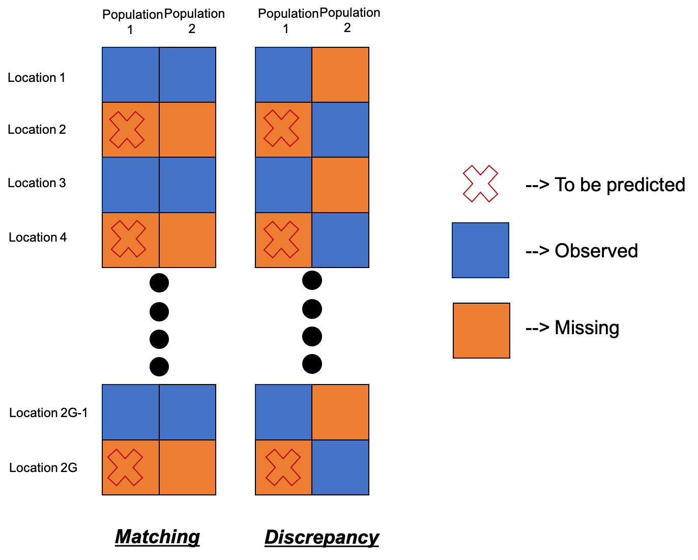
In this section, we further investigate when our proposal is expected to improve the accuracy of the missing data imputation. We conjecture that the strength of the cross-population dependence varies with the structure of the missing data. Considering two populations of a certain year, we define two extreme missing structures as follows:

•

Matching – at each location, the surveillance data of the two populations are either both available OR both missing;
•

Discrepancy – at each location, the surveillance data are available for one population AND missing for the other population.

A visual illustration is in Figure 5. The missing structure of real surveillance data for multiple populations is usually a mix of those two extremes. However, studying missing structure via focusing on the extreme cases make it efficient to evaluate their impact on missing imputation.

In the following two sections, we study the impacts of the two missing structures on two aspects: (1) imputation robustness and (2) statistical inference of population dependence parameter $\rho_{ii^{\prime}}$ . The relevant derivations and proofs are summarized in Section B of the supplementary materials.

5.1 Imputation Robustness

In this subsection, we investigate the impact of two missing data structures in Figure 5 on imputation robustness. For simplicity, we assume that there is only one year ( $K=1$ ), which means that the dummy index $k$ denoting the years is omitted in the following illustration. We evaluate the performance of imputation by treating crossed entries as the ones to be predicted. The missing entries are predicted by using predictive posterior density, and the densities under different missing structures are differently expressed. For the matching structure, the predictive posterior density depends on two components: the observations of population 1, denoted as $\bm{\mu}_{obs1}=[\mu_{11},\mu_{13},...,\mu_{1,(2G-1)}]^{T}$ , and the observations of population 2, denoted as $\bm{\mu}_{obs2}=[\mu_{21},\mu_{23},...,\mu_{2,(2G-1)}]^{T}$ . For the discrepancy structure, the predictive posterior density depends on two components: the observations of population 1, denoted as $\bm{\mu}_{obs1}=[\mu_{11},\mu_{13},...,\mu_{1,(2G-1)}]^{T}$ , and the observations of population 2, denoted as $\bm{\mu}_{obs2}=[\mu_{22},\mu_{24},...,\mu_{2,2G}]^{T}$ . For both cases, we aim to predict $\bm{\mu}_{pred}=[\mu_{12},\mu_{14},...,\mu_{1,2G}]^{T}$ . For a more concise illustration, we further assume fixed effects are zeros. Let $\bm{\Sigma}_{pred}=\bm{L}_{pred}\bm{L}_{pred}^{T}$ , $\bm{\Sigma}_{obs1}=\bm{L}_{obs1}\bm{L}_{obs1}^{T}$ , $\bm{\Sigma}_{obs2}=\bm{L}_{obs2}\bm{L}_{obs2}^{T}$ be the marginal covariance matrices of $\bm{\mu}_{pred},\bm{\mu}_{obs1},\bm{\mu}_{obs2}$ , respectively; $\rho$ be the population dependence parameter between population 1 and population 2. We express $\bm{\mu}_{pred},\bm{\mu}_{obs1},\bm{\mu}_{obs2}$ as

	$\displaystyle\text{Matching:}$	$\displaystyle\left\{\begin{aligned} \bm{\mu}_{pred}&=\bm{L}_{pred}(\bm{R}\bm{Z}_{1}+(\bm{I}-\bm{R}\bm{R}^{T})^{\frac{1}{2}}\bm{Z}_{2}),\\ \bm{\mu}_{obs1}&=\bm{L}_{obs1}\bm{Z}_{1},\\ \bm{\mu}_{obs2}&=\bm{L}_{obs2}(\rho\bm{Z}_{1}+(1-\rho^{2})^{\frac{1}{2}}\bm{Z}_{3}),\end{aligned}\right.$

	$\displaystyle\text{Discrepancy:}$	$\displaystyle\left\{\begin{aligned} \bm{\mu}_{pred}&=\bm{L}_{pred}\bm{Z}_{1},\\ \bm{\mu}_{obs1}&=\bm{L}_{obs1}(\bm{R}^{T}\bm{Z}_{1}+(\bm{I}-\bm{R}^{T}\bm{R})^{\frac{1}{2}}\bm{Z}_{2}),\\ \bm{\mu}_{obs2}&=\bm{L}_{obs2}(\rho\bm{Z}_{1}+(1-\rho^{2})^{\frac{1}{2}}\bm{Z}_{3}),\end{aligned}\right.$

where $\bm{R}=\bm{L}_{pred}^{-1}Cov(\bm{\mu}_{pred},\bm{\mu}_{obs1})(\bm{L}_{obs1}^{T})^{-1}$ , $\bm{Z}_{1}$ , $\bm{Z}_{2}$ and $\bm{Z}_{3}$ are independently distributed as a multivariate normal distribution with mean $\bm{0}$ and variance $\bm{I}$ , and $\bm{A}^{\frac{1}{2}}$ returns the lower Cholesky factor of $\bm{A}$ . Therefore, the joint distribution of $[\bm{\mu}_{pred},\bm{\mu}_{obs1},\bm{\mu}_{obs2}]$ is

$\displaystyle\text{Matching:}$	$\displaystyle\quad\left[\begin{bmatrix}\bm{\mu}_{pred}\\ \bm{\mu}_{obs1}\\ \bm{\mu}_{obs2}\end{bmatrix}\|.\right]\sim\mathcal{N}\left(\bm{0},\begin{bmatrix}\bm{\Sigma}_{pred}&\bm{L}_{pred}\bm{R}\bm{L}_{obs1}^{T}&\rho\bm{L}_{pred}\bm{R}\bm{L}_{obs2}^{T}\\ \bm{L}_{obs1}\bm{R}^{T}\bm{L}_{pred}^{T}&\bm{\Sigma}_{obs1}&\rho\bm{L}_{obs1}\bm{L}_{obs2}^{T}\\ \rho\bm{L}_{obs2}\bm{R}^{T}\bm{L}_{pred}^{T}&\rho\bm{L}_{obs2}\bm{L}_{obs1}^{T}&\bm{\Sigma}_{obs2}\end{bmatrix}\right)$	(2)
		(2)
$\displaystyle\text{Discrepancy:}$	$\displaystyle\quad\left[\begin{bmatrix}\bm{\mu}_{pred}\\ \bm{\mu}_{obs1}\\ \bm{\mu}_{obs2}\end{bmatrix}\|.\right]\sim\mathcal{N}\left(\bm{0},\begin{bmatrix}\bm{\Sigma}_{pred}&\bm{L}_{pred}\bm{R}\bm{L}_{obs1}^{T}&\rho\bm{L}_{pred}\bm{L}_{obs2}^{T}\\ \bm{L}_{obs1}\bm{R}^{T}\bm{L}_{pred}^{T}&\bm{\Sigma}_{obs1}&\rho\bm{L}_{obs1}\bm{R}^{T}\bm{L}_{obs2}^{T}\\ \rho\bm{L}_{obs2}\bm{L}_{pred}^{T}&\rho\bm{L}_{obs2}\bm{R}\bm{L}_{obs1}^{T}&\bm{\Sigma}_{obs2}\end{bmatrix}\right).$

Given the joint densities, we have the predictive posterior densities expressed as follows:

		$\displaystyle\text{Matching:}$		(3)
		$\displaystyle[\bm{\mu}_{pred}\|\bm{\mu}_{obs1},\bm{\mu}_{obs2},.]\sim\mathcal{N}[\bm{L}_{pred}\bm{R}\bm{L}_{obs1}^{T}\bm{\Sigma}_{obs1}^{-1}\bm{\mu}_{obs1},\bm{\Sigma}_{pred}-\bm{L}_{pred}\bm{R}\bm{R}^{T}\bm{L}_{pred}^{T}],$

		$\displaystyle\text{Discrepancy:}$
		$\displaystyle[\bm{\mu}_{pred}\|\bm{\mu}_{obs1},\bm{\mu}_{obs2},.]\sim\mathcal{N}[\bm{W}_{1}\bm{\mu}_{obs1}+\bm{W}_{2}\bm{\mu}_{obs2},\bm{\Sigma}_{pred}-(\bm{W}_{1}\bm{L}_{obs1}\bm{R}^{T}\bm{L}_{pred}^{T}+\bm{W}_{2}\bm{L}_{obs1}\bm{L}_{pred}^{T})],$

where

	$\displaystyle\bm{W}_{1}$	$\displaystyle=\bm{L}_{pred}\bm{R}(\bm{I}-\rho^{2}\bm{R}^{T}\bm{R})^{-1}\bm{L}_{obs1}^{-1}-\bm{L}_{pred}\rho^{2}(\bm{I}-\rho^{2}\bm{R}\bm{R}^{T})^{-1}\bm{R}\bm{L}_{obs1}^{-1},$		(4)
	$\displaystyle\bm{W}_{2}$	$\displaystyle=-\bm{L}_{pred}\rho\bm{R}\bm{R}^{T}(\bm{I}-\rho^{2}\bm{R}\bm{R}^{T})^{-1}\bm{L}_{obs2}^{-1}+\bm{L}_{pred}\rho(\bm{I}-\rho^{2}\bm{R}\bm{R}^{T})^{-1}\bm{L}_{obs2}^{-1}.$		(4)

In Equation (3), the discrepancy structure borrows information from both populations whereas the matching structure only borrows information from population 1. Thus the Bayesian estimation under the discrepancy structure utilizes more information, which is expected to perform better than that of the matching structure. Taking a closer look at the predictive distributions, we find that both predictive posterior densities enjoy unbiased mean after integrating out the observed ones, i.e., $\bm{\mu}_{obs1},\bm{\mu}_{obs2}$ . However, the discrepancy structure has a smaller predictive variance than that of the matching structure for any $\rho\in[-1,1]$ and the difference is larger if $|\rho|$ is closer to 1. The two variances are equal if and only if $\rho=0$ . Thus, $\rho$ controls how much information is borrowed from the dependent populations. In summary, we can give a remark below:

Remark 1.

The prediction of discrepancy structure is more robust than that of the matching structure. The prediction of discrepancy structure borrows information from both populations but the prediction of matching structure only borrows information from neighboring locations of its own population.

The relevant proof is in the Section B.1 of the supplementary materials. Here, we use a simple example to illustrate our claim. Let $G=1$ , Figure 6 illustrates the relationship between the predictive variance and the population dependence parameter under two missing data structures: discrepancy in blue and matching in yellow. We assume that the spatial covariance matrix of both population 1 and population 2 are $\bm{\Sigma}_{1}=\bm{\Sigma}_{2}=\begin{bmatrix}1&0.5\\ 0.5&1\end{bmatrix}$ . The discrepancy structure produces a smaller predictive variance when the absolute value of population dependence parameter is large. The population dependence parameter has no effect on the predictive variance of matching structure.

5.2 Population Dependence Parameter

As discussed in Section 5.1, the discrepancy structure provides a robust prediction. However, we also realize that this robustness relies on a valid statistical inference of the population dependence parameter $\rho$ . In this section, we discuss the impact of the missing structures on the estimation of the population dependence parameter $\rho$ . In particular, we compare the variances of the unbiased estimate, $\hat{\rho}=f(\bm{\mu}_{obs1},\bm{\mu}_{obs2})$ , under two missing data structures. Both $\bm{\mu}_{obs1}$ and $\bm{\mu}_{obs2}$ are observed ones as defined in Section 5.1. A lower bound on the variance of the unbiased estimator can be obtained by using the Cramér–Rao inequality (Gart 1959), such as $Var(\hat{\rho})\leq\mathcal{I}^{-1}(\rho)$ . Given a missing structure, the inverse of the Fisher information, $\mathcal{I}^{-1}(\rho)$ , is expressed as follows:

		$\displaystyle\text{Matching:}$		$\displaystyle\mathcal{I}_{Matching}^{-1}(\rho)=\frac{1}{G}\frac{(1-\rho^{2})^{2}}{1+\rho^{2}}.$		(5)
		$\displaystyle\text{Discrepancy:}$		$\displaystyle\mathcal{I}_{Discrepancy}^{-1}(\rho)=1/Tr[\rho\bm{R}^{T}(\bm{I}-\rho^{2}\bm{R}\bm{R}^{T})^{-1}\bm{R}]^{2}.$		(5)

The above information bounds are attained if $\frac{d}{d\rho}\log L(\rho|\bm{\mu}_{obs1},\bm{\mu}_{obs2})=a(\rho)(\hat{\rho}-\rho)$ where $a(\rho)$ is a function of $\rho$ and $\log L(\rho|\bm{\mu}_{obs1},\bm{\mu}_{obs2})$ is the log likelihood of $[\bm{\mu}_{obs1},\bm{\mu}_{obs2}]$ with ${Y}_{ijk}$ marginalized. In addition, $\mathcal{I}_{Matching}^{-1}(\rho)<\mathcal{I}_{Discrepancy}^{-1}(\rho)$ for any $\rho$ and $\bm{R}$ (See the proof in Supplement B.2). When $\bm{R}=\bm{0}$ , $\mathcal{I}_{Discrepancy}^{-1}(\rho)$ is infinity meaning that $\rho$ could not be estimated. In summary, we can give a remark below:

Remark 2.

The estimator of the population dependence parameter under the matching structure is more efficient than that under the discrepancy structure.

Figure 7 shows how $\mathcal{I}_{Matching}^{-1}(\rho)$ varies by $\rho$ and $G$ , which provides a way to control the variance of $\hat{\rho}$ in practice. For instance, if $|\rho|\geq 0.5$ , then observing data for both populations in $18$ locations could ensure $\mathcal{I}_{Matching}^{-1}(\rho)\leq 0.025$ . If we take $K$ years/replications into consideration, the inverted fisher information is $\frac{1}{G\times K}\frac{(1-\rho^{2})^{2}}{1+\rho^{2}}$ . This means the needed matching locations can be accumulative over the years. The examples we considered in this article satisfied this requirement.

To further validate Remark 2, we also numerically investigate how the spatial parameters affect the statistical inference of $\rho_{ii^{\prime}}$ . The simulated data are generated based on our proposed model (Equation 1). We use the map of Ukraine. We have $I=2$ , $J=27$ , and $K=10$ . For all $i,j,k$ , we have the sample size $N_{ijk}=100$ . We give the population-specific trends as $v_{1}(k)=\sin(0.2k)$ and $v_{2}(k)=\cos(0.2k)$ . The population-specific random effects are generated as $\bm{s}_{i}\sim\mathcal{N}(\bm{0},\bm{S})$ . The parameters associated with $\bm{S}$ are specified as follows. The population-specific spatial parameters are specified as $\sigma_{1}^{2}=\sigma_{2}^{2}=1$ . For each run, we sample a simulated data as follows, we simulate $50$ replications with $\rho_{12}\in\{0.1,0.2,...,0.9\}$ and $\phi_{1}=\phi_{2}\in\{0.2,0.3,...,0.6,0.7\}$ and hide the assumed missing entries as presented in Figure 5. From Figure 8, we can find that the MSE of posterior mean of $\rho$ is large under the structure of discrepancy. The MSE increases if the absolute value of $\rho$ is large. However, the structure of matching does not impact the posterior mean of $\rho_{12}$ . All these are consistent with our previous claims using Cramér–Rao inequality (Gart 1959).

5.3 Missing Structure Trade-Off

Putting Remarks 1 and 2 together, we found a trade-off between two missing structures: The matching structure gives an efficient estimation of population dependence parameter, but its prediction does not use the cross-population information v.s. The discrepancy structure gives a robust prediction by borrowing cross-population information but leads to inefficient estimation of the population dependence parameter. Given that the cross-population dependence induced by the Gaussian cosimulation (Oliver 2003) has a variety of applications environment (Recta et al. 2012; Fanshawe and Diggle 2012, e.g.,), this trade-off helps understand the strength and limitation of this model in terms of missing data imputation.

6 Conclusion and Discussion

Understanding HIV prevalence among key populations is important for HIV prevention. However, accurate estimates have been difficult to obtain because their HIV surveillance data is very limited. In this paper, we propose a generalized liner mixed model with the spatial conditional auto-regressive feature which captures both the spatial dependence and the cross-population dependence. The proposed model fully utilizes existing data and provides a useful statistical tool for HIV epidemiologists to impute the unknown prevalence rates and reveal potential spatial/cross-population variation. A substantial improvement in data imputation is obtained in the real data application, primarily resolving our scientific goal of estimating the HIV prevalence rates among key populations. The study also motivates us to explore the impact of missing data on imputation accuracy. We present both simulation results and theoretical results to reveal the strength and limitation of Gaussian cosimulation when the model is applied to the missing data imputation.

Two topics are worthwhile for further investigation. The first one is the cross-population dependence. Our proposal adopts Gaussian cosimulation (Oliver 2003), and the correlation parameter describes a linear relationship between the processes of any two populations. However, the actual cross-population dependence may be more complicated than the one we have proposed. Modern statistical methods such as graphical models may be implemented for handling the cross-population dependence, but the limited availability of our surveillance data may be a hurdle. The second one is the data missing mechanism. The missing entries are not missing completely at random but due to some specific reasons (e.g., resource allocation, administrative issues). It would be useful to know why the HIV surveillance data were missing for some combinations of key population, year and location, so that the potential bias due to missing not at random could be addressed. Unfortunately, such information is not readily available.

Supplementary Materials

A Codes

We compile our codes into an R package JointSpCAR. The package provides a function JointCAR() to implement our proposal. We also provide an R markdown script implantation.rmd introducing the function implementation by using synthetic HIV epidemic data. In addition, we also give the functions which are CAR() and Mixed(). They implement the benchmark methods which are the CAR model and Mixed model, respectively.

B Proofs

In this section, we give essential proofs of this article.

B.1 Proofs for Section 5.1 Imputation Robustness

In this subsection, we give the proofs for Section 5.1 Imputation Robustness. We give that $\bm{S}_{11}=Var(\bm{\mu}_{pred})$ , $\bm{S}_{22}=Var([\bm{\mu}_{obs1}^{T},\bm{\mu}_{obs2}^{T}]^{T})$ , and $\bm{S}_{12}=Cov(\bm{\mu}_{pred},[\bm{\mu}_{obs1}^{T},\bm{\mu}_{obs2}^{T}]^{T})$ . Thus, for both structures, the posterior mean is $\bm{S}_{12}\bm{S}_{22}^{-1}[\bm{\mu}_{obs1}^{T},\bm{\mu}_{obs2}^{T}]^{T}$ and the posterior variance matrix is $\bm{S}_{11}-\bm{S}_{12}\bm{S}_{22}^{-1}\bm{S}_{12}^{T}$ .

The bottleneck of obtaining the mean and the variance is $\bm{S}_{22}^{-1}$ . Lu and Shiou 2002 gives an explicit inverse formula for a $2\times 2$ block matrix, which is summarized in Theorem 1:

Theorem 1.

Let $\bm{R}=\begin{bmatrix}\bm{A}&\bm{B}\\ \bm{C}&\bm{D}\end{bmatrix}$ be a square positive semi-definite matrix where $\bm{A}$ and $\bm{D}$ are all square matrices. Let $\bm{R}^{-1}=\begin{bmatrix}\bm{E}&\bm{F}\\ \bm{G}&\bm{H}\end{bmatrix}$ be inversion of $\bm{R}$ and the components in the inversion are

•

$\bm{E}=\bm{A}^{-1}+\bm{A}^{-1}\bm{B}(\bm{D}-\bm{C}\bm{A}^{-1}\bm{B})^{-1}\bm{C}\bm{A}^{-1}$
•

$\bm{F}=-\bm{A}^{-1}\bm{B}(\bm{D}-\bm{C}\bm{A}^{-1}\bm{B})^{-1}$
•

$\bm{G}=-(\bm{D}-\bm{C}\bm{A}^{-1}\bm{B})\bm{C}\bm{A}^{-1}$
•

$\bm{H}=(\bm{D}-\bm{C}\bm{A}^{-1}\bm{B})^{-1}$

Next, we apply Theorem 1 to both structures:

Matching Structure:

Here, we give that $\bm{A}=\bm{\Sigma}_{obs1}$ , $\bm{B}=\rho\bm{L}_{obs1}\bm{L}_{obs2}^{T}$ , $\bm{C}=\rho\bm{L}_{obs2}\bm{L}_{obs1}^{T}$ , and $\bm{D}=\bm{\Sigma}_{obs2}$ . Then, $\bm{E}$ , $\bm{F}$ , $\bm{G}$ , and $\bm{H}$ are expressed as follows:

	$\displaystyle\bm{E}$	$\displaystyle=\bm{A}^{-1}+\bm{A}^{-1}\bm{B}(\bm{D}-\bm{C}\bm{A}^{-1}\bm{B})^{-1}\bm{C}\bm{A}^{-1}$
		$\displaystyle=\bm{\Sigma}_{obs1}^{-1}+\bm{\Sigma}_{obs1}^{-1}\rho\bm{L}_{obs1}\bm{L}_{obs2}^{T}(\bm{\Sigma}_{obs2}-\rho\bm{L}_{obs2}\bm{L}_{obs1}^{T}\bm{\Sigma}_{obs1}^{-1}\rho\bm{L}_{obs1}\bm{L}_{obs2}^{T})^{-1}\rho\bm{L}_{obs2}\bm{L}_{obs1}^{T}\bm{\Sigma}_{obs1}^{-1}$
		$\displaystyle=\frac{1}{1-\rho^{2}}\bm{\Sigma}_{obs1}^{-1}$

	$\displaystyle\bm{F}$	$\displaystyle=-\bm{A}^{-1}\bm{B}(\bm{D}-\bm{C}\bm{A}^{-1}\bm{B})^{-1}$
		$\displaystyle=-\bm{\Sigma}_{obs1}^{-1}\rho\bm{L}_{obs1}\bm{L}_{obs2}^{T}(\bm{\Sigma}_{obs2}-\rho\bm{L}_{obs2}\bm{L}_{obs1}^{T}\bm{\Sigma}_{obs1}^{-1}\rho\bm{L}_{obs1}\bm{L}_{obs2}^{T})^{-1}$
		$\displaystyle=-\bm{\Sigma}_{obs1}^{-1}\bm{L}_{obs1}\bm{L}_{obs2}^{T}\bm{\Sigma}_{obs2}^{-1}\frac{\rho}{1-\rho^{2}}$

	$\displaystyle\bm{G}$	$\displaystyle=-\bm{\Sigma}_{obs2}^{-1}\bm{L}_{obs2}\bm{L}_{obs1}^{T}\bm{\Sigma}_{obs1}^{-1}\frac{\rho}{1-\rho^{2}}$

	$\displaystyle\bm{H}$	$\displaystyle=(\bm{D}-\bm{C}\bm{A}^{-1}\bm{B})^{-1}$
		$\displaystyle=(\bm{\Sigma}_{obs2}-\rho\bm{L}_{obs2}\bm{L}_{obs1}^{T}\bm{\Sigma}_{obs1}^{-1}\rho\bm{L}_{obs1}\bm{L}_{obs2}^{T})^{-1}$
		$\displaystyle=\frac{1}{1-\rho^{2}}\bm{\Sigma}_{obs2}^{-1}$

Then the posterior mean is

		$\displaystyle\bm{S}_{12}\bm{S}_{22}^{-1}[\bm{\mu}_{obs1}^{T},\bm{\mu}_{obs2}^{T}]^{T}$
		$\displaystyle=[\bm{L}_{pred}\bm{R}\bm{L}_{obs1}^{T},\ \rho\bm{L}_{pred}\bm{R}\bm{L}_{obs2}^{T}]\begin{bmatrix}\frac{1}{1-\rho^{2}}\bm{\Sigma}_{obs1}^{-1}&-\bm{\Sigma}_{obs1}^{-1}\bm{L}_{obs1}\bm{L}_{obs2}^{T}\bm{\Sigma}_{obs2}^{-1}\frac{\rho}{1-\rho^{2}}\\ -\bm{\Sigma}_{obs2}^{-1}\bm{L}_{obs2}\bm{L}_{obs1}^{T}\bm{\Sigma}_{obs1}^{-1}\frac{\rho}{1-\rho^{2}}&\frac{1}{1-\rho^{2}}\bm{\Sigma}_{obs2}^{-1}\end{bmatrix}\begin{bmatrix}\bm{\mu}_{obs1}\\ \bm{\mu}_{obs2}\end{bmatrix}$
		$\displaystyle=\bm{L}_{pred}\bm{R}\bm{L}_{obs1}^{T}\bm{\Sigma}_{obs1}^{-1}\bm{\mu}_{obs1},$

and the posterior variance is

		$\displaystyle\bm{S}_{11}-\bm{S}_{12}\bm{S}_{22}^{-1}\bm{S}_{12}^{T}$
		$\displaystyle=\bm{\Sigma}_{pred}-$
		$\displaystyle[\bm{L}_{pred}\bm{R}\bm{L}_{obs1}^{T},\ \rho\bm{L}_{pred}\bm{R}\bm{L}_{obs2}^{T}]\begin{bmatrix}\frac{1}{1-\rho^{2}}\bm{\Sigma}_{obs1}^{-1}&-\bm{\Sigma}_{obs1}^{-1}\bm{L}_{obs1}\bm{L}_{obs2}^{T}\bm{\Sigma}_{obs2}^{-1}\frac{\rho}{1-\rho^{2}}\\ -\bm{\Sigma}_{obs2}^{-1}\bm{L}_{obs2}\bm{L}_{obs1}^{T}\bm{\Sigma}_{obs1}^{-1}\frac{\rho}{1-\rho^{2}}&\frac{1}{1-\rho^{2}}\bm{\Sigma}_{obs2}^{-1}\end{bmatrix}\begin{bmatrix}\bm{L}_{obs1}\bm{R}^{T}\bm{L}_{pred}^{T}\\ \rho\bm{L}_{obs2}\bm{R}^{T}\bm{L}_{pred}^{T}\end{bmatrix}$
		$\displaystyle=\bm{\Sigma}_{pred}-[\bm{L}_{pred}\bm{R}\bm{L}_{obs1}^{T}\bm{\Sigma}_{obs1}^{-1},\bm{0}]\begin{bmatrix}\bm{L}_{obs1}\bm{R}^{T}\bm{L}_{pred}^{T}\\ \rho\bm{L}_{obs2}\bm{R}^{T}\bm{L}_{pred}^{T}\end{bmatrix}$
		$\displaystyle=\bm{\Sigma}_{pred}-\bm{L}_{pred}\bm{R}\bm{R}^{T}\bm{L}_{pred}^{T}$

Discrepancy Structure:

Here, we give that $\bm{A}=\bm{\Sigma}_{obs1}$ , $\bm{B}=\rho\bm{L}_{obs1}\bm{R}^{T}\bm{L}_{obs2}^{T}$ , $\bm{C}=\rho\bm{L}_{obs2}\bm{R}\bm{L}_{obs1}^{T}$ , and $\bm{D}=\bm{\Sigma}_{obs2}$ . Then, $\bm{E}$ , $\bm{F}$ , $\bm{G}$ , and $\bm{H}$ are expressed as follows:

	$\displaystyle\bm{E}$	$\displaystyle=\bm{A}^{-1}+\bm{A}^{-1}\bm{B}(\bm{D}-\bm{C}\bm{A}^{-1}\bm{B})^{-1}\bm{C}\bm{A}^{-1}$
		$\displaystyle=\bm{\Sigma}_{obs1}^{-1}+\bm{\Sigma}_{obs1}^{-1}\rho\bm{L}_{obs1}\bm{R}^{T}\bm{L}_{obs2}^{T}(\bm{\Sigma}_{obs2}-\rho\bm{L}_{obs2}\bm{R}\bm{L}_{obs1}^{T}\bm{\Sigma}_{obs1}^{-1}\rho\bm{L}_{obs1}\bm{R}\bm{L}_{obs2}^{T})^{-1}\rho\bm{L}_{obs2}\bm{R}\bm{L}_{obs1}^{T}\bm{\Sigma}_{obs1}^{-1}$
		$\displaystyle=(\bm{\Sigma}_{obs1}-\rho^{2}\bm{L}_{obs1}\bm{R}^{T}\bm{R}\bm{L}_{obs1}^{T})^{-1}$

	$\displaystyle\bm{F}$	$\displaystyle=-\bm{A}^{-1}\bm{B}(\bm{D}-\bm{C}\bm{A}^{-1}\bm{B})^{-1}$
		$\displaystyle=-\bm{\Sigma}_{obs1}^{-1}\rho\bm{L}_{obs1}\bm{R}^{T}\bm{L}_{obs2}^{T}(\bm{\Sigma}_{obs2}-\rho\bm{L}_{obs2}\bm{R}\bm{L}_{obs1}^{T}\bm{\Sigma}_{obs1}^{-1}\rho\bm{L}_{obs1}\bm{R}^{T}\bm{L}_{obs2}^{T})^{-1}$
		$\displaystyle=-\bm{\Sigma}_{obs1}^{-1}\rho\bm{L}_{obs1}\bm{R}^{T}\bm{L}_{obs2}^{T}(\bm{\Sigma}_{obs2}-\rho^{2}\bm{L}_{obs2}\bm{R}\bm{R}^{T}\bm{L}_{obs2}^{T})^{-1}$
		$\displaystyle=-\rho(\bm{L}_{obs1}^{T})^{-1}\bm{R}^{T}(\bm{I}-\rho^{2}\bm{R}\bm{R}^{T})^{-1}\bm{L}_{obs2}^{-1}$

	$\displaystyle\bm{G}$	$\displaystyle=-\rho(\bm{L}_{obs2}^{T})^{-1}(\bm{I}-\rho^{2}\bm{R}\bm{R}^{T})^{-1}\bm{R}\bm{L}_{obs1}^{-1}$

	$\displaystyle\bm{H}$	$\displaystyle=(\bm{D}-\bm{C}\bm{A}^{-1}\bm{B})^{-1}$
		$\displaystyle=(\bm{\Sigma}_{obs2}-\rho\bm{L}_{obs2}\bm{R}\bm{L}_{obs1}^{T}\bm{\Sigma}_{obs1}^{-1}\rho\bm{L}_{obs1}\bm{R}^{T}\bm{L}_{obs2}^{T})^{-1}$
		$\displaystyle=(\bm{\Sigma}_{obs2}-\rho^{2}\bm{L}_{obs2}\bm{R}\bm{R}^{T}\bm{L}_{obs2}^{T})^{-1}$

Then the posterior mean is

		$\displaystyle\bm{S}_{12}\bm{S}_{22}^{-1}[\bm{\mu}_{obs1}^{T},\bm{\mu}_{obs2}^{T}]^{T}$
		$\displaystyle=[\bm{L}_{pred}\bm{R}\bm{L}_{obs1}^{T},\ \rho\bm{L}_{pred}\bm{L}_{obs2}^{T}]$
		$\displaystyle\begin{bmatrix}(\bm{\Sigma}_{obs1}-\rho^{2}\bm{L}_{obs1}\bm{R}^{T}\bm{R}\bm{L}_{obs1}^{T})^{-1}&-\rho(\bm{L}_{obs1}^{T})^{-1}\bm{R}^{T}(\bm{I}-\rho^{2}\bm{R}\bm{R}^{T})^{-1}\bm{L}_{obs2}^{-1}\\ -\rho(\bm{L}_{obs2}^{T})^{-1}(\bm{I}-\rho^{2}\bm{R}\bm{R}^{T})^{-1}\bm{R}\bm{L}_{obs1}^{-1}&(\bm{\Sigma}_{obs2}-\rho^{2}\bm{L}_{obs2}\bm{R}\bm{R}^{T}\bm{L}_{obs2}^{T})^{-1}\end{bmatrix}\begin{bmatrix}\bm{\mu}_{obs1}\\ \bm{\mu}_{obs2}\end{bmatrix}$
		$\displaystyle=\bm{W}_{1}\bm{\mu}_{obs1}+\bm{W}_{2}\bm{\mu}_{obs2},$

where

	$\displaystyle\bm{W}_{1}$	$\displaystyle=\bm{L}_{pred}\bm{R}(\bm{I}-\rho^{2}\bm{R}^{T}\bm{R})^{-1}\bm{L}_{obs1}^{-1}-\bm{L}_{pred}\rho^{2}(\bm{I}-\rho^{2}\bm{R}\bm{R}^{T})^{-1}\bm{R}\bm{L}_{obs1}^{-1}$
	$\displaystyle\bm{W}_{2}$	$\displaystyle=-\bm{L}_{pred}\rho\bm{R}\bm{R}^{T}(\bm{I}-\rho^{2}\bm{R}\bm{R}^{T})^{-1}\bm{L}_{obs2}^{-1}+\bm{L}_{pred}\rho(\bm{I}-\rho^{2}\bm{R}\bm{R}^{T})^{-1}\bm{L}_{obs2}^{-1}$

and the posterior variance is

		$\displaystyle\bm{S}_{11}-\bm{S}_{12}\bm{S}_{22}^{-1}\bm{S}_{12}^{T}$
		$\displaystyle=\bm{\Sigma}_{pred}-[\bm{W}_{1}\ \bm{W}_{2}]\begin{bmatrix}\bm{L}_{obs1}\bm{R}^{T}\bm{L}_{pred}^{T}\\ \rho\bm{L}_{obs2}\bm{L}_{pred}^{T}\end{bmatrix}$
		$\displaystyle=\bm{\Sigma}_{pred}-$
		$\displaystyle[\bm{L}_{pred}\bm{R}(\bm{I}-\rho^{2}\bm{R}^{T}\bm{R})^{-1}\bm{R}^{T}\bm{L}_{pred}^{T}-\bm{L}_{pred}\rho^{2}(\bm{I}-\rho^{2}\bm{R}\bm{R}^{T})^{-1}\bm{R}\bm{R}^{T}\bm{L}_{pred}^{T}-$
		$\displaystyle\bm{L}_{pred}\rho\bm{R}\bm{R}^{T}(\bm{I}-\rho^{2}\bm{R}\bm{R}^{T})^{-1}\rho\bm{L}_{pred}^{T}+\bm{L}_{pred}\rho(\bm{I}-\rho^{2}\bm{R}\bm{R}^{T})^{-1}\rho\bm{L}_{pred}^{T}]$

Next, we want to prove that the predictive variance of the matching structure is larger than that of discrepancy structure, that is

\displaystyle\Delta\bm{S}=\bm{S}_{Matching}-\bm{S}_{Discrepancy}\succeq\bm{0},

where $\bm{S}_{Matching}$ and $\bm{S}_{Discrepancy}$ are the conditional covariance matrices of the matching structure and discrepancy structure, respectively. This is also equivalent to show that

		$\displaystyle\bm{U}=$
		$\displaystyle[{\bm{R}(\bm{I}-\rho^{2}\bm{R}^{T}\bm{R})^{-1}\bm{R}^{T}}-{\rho^{2}(\bm{I}-\rho^{2}\bm{R}\bm{R}^{T})^{-1}\bm{R}\bm{R}^{T}}-{\rho\bm{R}\bm{R}^{T}(\bm{I}-\rho^{2}\bm{R}\bm{R}^{T})^{-1}\rho}+{\rho(\bm{I}-\rho^{2}\bm{R}\bm{R}^{T})^{-1}\rho}]-{\bm{R}\bm{R}^{T}}$
		$\displaystyle\succeq\bm{0}$

for all $\rho\in[-1,1]$ and $\bm{R}$ . Given the Neumann series, $\bm{U}$ can be expressed as

$\displaystyle\bm{U}$	$\displaystyle=\bm{R}\sum_{k=0}^{\infty}(\rho^{2}\bm{R}^{T}\bm{R})^{k}\bm{R}^{T}-\rho^{2}\sum_{k=0}^{\infty}(\rho^{2}\bm{R}\bm{R}^{T})^{k}\bm{R}\bm{R}^{T}-\rho^{2}\bm{R}\bm{R}^{T}\sum_{k=0}^{\infty}(\rho^{2}\bm{R}\bm{R}^{T})^{k}+\rho^{2}\sum_{k=0}^{\infty}(\rho^{2}\bm{R}\bm{R}^{T})^{k}-\bm{R}\bm{R}^{T}$	(6)
	$\displaystyle=\bm{R}\sum_{k=0}^{\infty}(\rho^{2}\bm{R}^{T}\bm{R})^{k}\bm{R}^{T}-2\rho^{2}\sum_{k=0}^{\infty}(\rho^{2})^{k}(\bm{R}\bm{R}^{T})^{k+1}+\rho^{2}\sum_{k=0}^{\infty}(\rho^{2}\bm{R}\bm{R}^{T})^{k}-\bm{R}\bm{R}^{T}$
	$\displaystyle=\sum_{k=1}^{\infty}(\rho^{2})^{k}(\bm{R}\bm{R}^{T})^{k+1}-2\rho^{2}\sum_{k=0}^{\infty}(\rho^{2})^{k}(\bm{R}\bm{R}^{T})^{k+1}+\rho^{2}\sum_{k=0}^{\infty}(\rho^{2}\bm{R}\bm{R}^{T})^{k}$
	$\displaystyle=\sum_{k=1}^{\infty}(\rho^{2})^{k}(\bm{R}\bm{R}^{T})^{k+1}-2\rho^{2}\sum_{k=1}^{\infty}(\rho^{2})^{k-1}(\bm{R}\bm{R}^{T})^{k}+\rho^{2}\sum_{k=1}^{\infty}(\rho^{2}\bm{R}\bm{R}^{T})^{k-1}$
	$\displaystyle=\sum_{k=1}^{\infty}\rho^{2k}\bm{Z}^{k-1}(\bm{I}-\bm{Z})^{2},$

where $\bm{Z}=\bm{R}\bm{R}^{T}$ . Because $\bm{Z}^{k-1}(\bm{I}-\bm{Z})^{2}$ is positive semi-definite for all $k$ , then $\bm{U}$ is positive semi-definite. In summary, we proved our statement.

B.2 Proofs for Section 5.2 Population Dependence Parameter

In this subsection, we give the proofs for Section 5.2 Population Dependence Parameter. The Fisher information $\mathcal{I}(\rho)$ (Malagò and Pistone 2015) is

\displaystyle\mathcal{I}(\rho)=\frac{1}{2}Tr(\bm{S}_{22}^{-1}\frac{\partial\bm{S}_{22}}{\partial\rho}\bm{S}_{22}^{-1}\frac{\partial\bm{S}_{22}}{\partial\rho}).

(7)

We have already given the expressions of $\bm{S}_{22}^{-1}$ and $\bm{S}_{22}$ in Section B.1. Thus, it is not difficult to give explicit expression of these $\mathcal{I}(\rho)$ by plugging in the expressions of $\bm{S}_{22}^{-1}$ and $\bm{S}_{22}$ under matching structure or discrepancy structure.

Next, we want to prove $\mathcal{I}_{Matching}^{-1}(\rho)<\mathcal{I}_{Discrepancy}^{-1}(\rho)$ for any $\rho$ and $\bm{R}$ . Our goal is to find a lower bond of $\mathcal{I}_{Discrepancy}^{-1}(\rho)$ . Given the Neumann series, $\mathcal{I}_{Discrepancy}^{-1}(\rho)$ can be expressed as

	$\displaystyle\mathcal{I}_{Discrepancy}^{-1}(\rho)$	$\displaystyle=1/Tr[\rho\bm{R}^{T}(\bm{I}-\rho^{2}\bm{R}\bm{R}^{T})^{-1}\bm{R}]^{2}$
		$\displaystyle=1/Tr[\rho\bm{R}\sum_{k=0}^{\infty}(\rho^{2}\bm{R}^{T}\bm{R})^{k}\bm{R}^{T}]^{2}$
		$\displaystyle=1/Tr[\rho\sum_{k=0}^{\infty}(\rho^{2})^{k}(\bm{R}\bm{R}^{T})^{k+1}]^{2}$
		$\displaystyle=1/Tr\left[\rho^{2}\left(\sum_{k=0}^{\infty}(\rho^{2})^{2k}(\bm{R}\bm{R}^{T})^{2(k+1)}+\sum_{i\not=j}^{0:\infty}(\rho^{2})^{i}(\bm{R}\bm{R}^{T})^{i+1}(\rho^{2})^{j}(\bm{R}\bm{R}^{T})^{j+1}\right)\right]$

Because all the eigenvalues of $\bm{R}$ are less than 1, then $Tr(\bm{R}\bm{R}^{T})^{k}<G$ for any $k$ . Thus, the lower bond of $\mathcal{I}_{Discrepancy}^{-1}(\rho)$ is $\frac{1}{G}\frac{(1-\rho^{2})^{2}}{\rho^{2}}$ which is larger than $\mathcal{I}_{Matching}^{-1}(\rho)$ . Thus, we proved that $\mathcal{I}_{Matching}^{-1}(\rho)<\mathcal{I}_{Discrepancy}^{-1}(\rho)$ for any $\rho$ and $\bm{R}$ .

References

(1)
Alfvén et al. (2017) Alfvén, T., Erkkola, T., Ghys, P., Padayachy, J., Warner-Smith, M., Rugg, D. and De Lay, P. (2017), ‘Global AIDS reporting-2001 to 2015: lessons for monitoring the sustainable development goals’, AIDS and Behavior 21(1), 5–14.
Bao et al. (2012) Bao, L., Salomon, J. A., Brown, T., Raftery, A. E. and Hogan, D. R. (2012), ‘Modelling national HIV/AIDS epidemics: revised approach in the unAIDS estimation and projection package 2011’, Sexually Transmitted Infections 88(Suppl 2), i3–i10.
Baral et al. (2012) Baral, S., Beyrer, C., Muessig, K., Poteat, T., Wirtz, A. L., Decker, M. R., Sherman, S. G. and Kerrigan, D. (2012), ‘Burden of HIV among female sex workers in low-income and middle-income countries: a systematic review and meta-analysis’, The Lancet Infectious Diseases 12(7), 538–549.
Bekker et al. (2018) Bekker, L.-G., Alleyne, G., Baral, S., Cepeda, J., Daskalakis, D., Dowdy, D., Dybul, M., Eholie, S., Esom, K., Garnett, G. et al. (2018), ‘Advancing global health and strengthening the HIV response in the era of the sustainable development goals: the international AIDS society—lancet commission’, The Lancet 392(10144), 312–358.
Besag (1974) Besag, J. (1974), ‘Spatial interaction and the statistical analysis of lattice systems’, Journal of the Royal Statistical Society: Series B (Methodological) 36(2), 192–225.
Calleja et al. (2010) Calleja, J. M. G., Jacobson, J., Garg, R., Thuy, N., Stengaard, A., Alonso, M., Ziady, H., Mukenge, L., Ntabangana, S., Chamla, D. et al. (2010), ‘Has the quality of serosurveillance in low-and middle-income countries improved since the last HIV estimates round in 2007? status and trends through 2009’, Sexually Transmitted Infections 86(Suppl 2), ii35–ii42.
de Valpine et al. (2017) de Valpine, P., Turek, D., Paciorek, C. J., Anderson-Bergman, C., Lang, D. T. and Bodik, R. (2017), ‘Programming with models: writing statistical algorithms for general model structures with nimble’, Journal of Computational and Graphical Statistics 26(2), 403–413.
Eaton et al. (2019) Eaton, J. W., Brown, T., Puckett, R., Glaubius, R., Mutai, K., Bao, L., Salomon, J. A., Stover, J., Mahy, M. and Hallett, T. B. (2019), ‘The estimation and projection package age-sex model and the r-hybrid model: new tools for estimating HIV incidence trends in sub-saharan africa’.
Eaton et al. (2011) Eaton, J. W., Hallett, T. B. and Garnett, G. P. (2011), ‘Concurrent sexual partnerships and primary HIV infection: a critical interaction’, AIDS and Behavior 15(4), 687–692.
Fanshawe and Diggle (2012) Fanshawe, T. R. and Diggle, P. J. (2012), ‘Bivariate geostatistical modelling: a review and an application to spatial variation in radon concentrations’, Environmental and Ecological Statistics 19(2), 139–160.
Gart (1959) Gart, J. J. (1959), ‘An extension of the cramér-rao inequality’, The Annals of Mathematical Statistics pp. 367–380.
Gasch et al. (2015) Gasch, C. K., Hengl, T., Gräler, B., Meyer, H., Magney, T. S. and Brown, D. J. (2015), ‘Spatio-temporal interpolation of soil water, temperature, and electrical conductivity in 3d+ t: The cook agronomy farm data set’, Spatial Statistics 14, 70–90.
Gelman et al. (2013) Gelman, A., Carlin, J. B., Stern, H. S., Dunson, D. B., Vehtari, A. and Rubin, D. B. (2013), Bayesian Data Analysis, CRC press.
Lee (2013) Lee, D. (2013), ‘Carbayes: an r package for bayesian spatial modeling with conditional autoregressive priors’, Journal of Statistical Software 55(13), 1–24.
Lu and Shiou (2002) Lu, T.-T. and Shiou, S.-H. (2002), ‘Inverses of 2 $\times$ 2 block matrices’, Computers & Mathematics with Applications 43(1-2), 119–129.
Lyerla et al. (2008) Lyerla, R., Gouws, E. and Garcia-Calleja, J. (2008), ‘The quality of sero-surveillance in low-and middle-income countries: status and trends through 2007’, Sexually Transmitted Infections 84(Suppl 1), i85–i91.
Malagò and Pistone (2015) Malagò, L. and Pistone, G. (2015), Information geometry of the gaussian distribution in view of stochastic optimization, in ‘Proceedings of the 2015 ACM Conference on Foundations of Genetic Algorithms XIII’, pp. 150–162.
Meyer et al. (2016) Meyer, H., Katurji, M., Appelhans, T., Müller, M. U., Nauss, T., Roudier, P. and Zawar-Reza, P. (2016), ‘Mapping daily air temperature for antarctica based on modis lst’, Remote Sensing 8(9), 732.
Meyer et al. (2018) Meyer, H., Reudenbach, C., Hengl, T., Katurji, M. and Nauss, T. (2018), ‘Improving performance of spatio-temporal machine learning models using forward feature selection and target-oriented validation’, Environmental Modelling & Software 101, 1–9.
Naghavi et al. (2017) Naghavi, M., Abajobir, A. A., Abbafati, C., Abbas, K. M., Abd-Allah, F., Abera, S. F., Aboyans, V., Adetokunboh, O., Afshin, A., Agrawal, A. et al. (2017), ‘Global, regional, and national age-sex specific mortality for 264 causes of death, 1980–2016: a systematic analysis for the global burden of disease study 2016’, The Lancet 390(10100), 1151–1210.
Niu et al. (2017) Niu, X., Zhang, A., Brown, T., Puckett, R., Mahy, M. and Bao, L. (2017), ‘Incorporation of hierarchical structure into estimation and projection package fitting with examples of estimating subnational HIV/AIDS dynamics’, AIDS 31(1), S51–S59.
Oliver (2003) Oliver, D. S. (2003), ‘Gaussian cosimulation: modelling of the cross-covariance’, Mathematical Geology 35(6), 681–698.
Recta et al. (2012) Recta, V., Haran, M. and Rosenberger, J. L. (2012), ‘A two-stage model for incidence and prevalence in point-level spatial count data’, Environmetrics 23(2), 162–174.
Rue and Held (2005) Rue, H. and Held, L. (2005), Gaussian Markov Random Fields: Theory and Applications, CRC press.
Spiegel (2004) Spiegel, P. B. (2004), ‘HIV/AIDS among conflict-affected and displaced populations: Dispelling myths and taking action’, Disasters 28(3), 322–339.
Weatherill et al. (2015) Weatherill, G., Silva, V., Crowley, H. and Bazzurro, P. (2015), ‘Exploring the impact of spatial correlations and uncertainties for portfolio analysis in probabilistic seismic loss estimation’, Bulletin of Earthquake Engineering 13(4), 957–981.
World Health Organization (2019) World Health Organization (2019), The global action plan for healthy lives and well-being for all: strengthening collaboration among multilateral organizations to accelerate country progress on the health-related sustainable development goals, Technical report, WHO.
Xue et al. (2018) Xue, W., Bowman, F. D. and Kang, J. (2018), ‘A Bayesian spatial model to predict disease status using imaging data from various modalities’, Frontiers in Neuroscience 12, 184.