跳到论文正文
W Papers独立论文阅读器 arXiv:2009.01055 论文正文 计算阅读时间 · 0%
引用这篇论文根据当前论文元数据生成,正式投稿前建议核对。


License: arXiv.org perpetual non-exclusive license
arXiv:2009.01055v1 [math.DS] 02 Sep 2020

Space-PCE POD for PDEs with Uncertainties

\msc

35R60, 60H35, 65N22

Space and Chaos-Expansion Galerkin POD Low-order Discretization of PDEs for Uncertainty Quantification

Peter Benner    Jan Heiland
Abstract

The quantification of multivariate uncertainties in partial differential equations can easily exceed any computing capacity unless proper measures are taken to reduce the complexity of the model. In this work, we propose a multidimensional Galerkin Proper Orthogonal Decomposition that optimally reduces each dimension of a tensorized product space. We provide the analytical framework and results that define and quantify the low-dimensional approximation. We illustrate its application for uncertainty modeling with Polynomial Chaos Expansions and show its efficiency in a numerical example.

keywords
uncertainty quantification, model reduction, Proper Orthogonal Decomposition, tensor spaces

1 Introduction

The statistically sound treatment of modeled uncertainties in simulations comes with significant additional computational costs. Since a deterministic model can already be arbitrarily complex, the computation of statistics for general problems may soon become infeasible unless some kind of model reduction is involved.

In this work, we propose a multidimensional Galerkin POD that can simultaneously and optimally reduces the physical dimensions of the model and the dimensions related to the uncertainties.

For the quantification of uncertainties in PDE models and their numerical discretization, one may distinguish two categories of solvers [18] – sampling based methods, notably the Monte-Carlo method, and Galerkin-type projection methods. In this work, we focus on the latter. For a basic explanation and relevant references on the Monte-Carlo method and its extensions see [18], for an application in elliptic PDEs see [8], and for a combination with stochastic collocation and tensor techniques see [13].

Galerkin-type methods for solving PDEs with uncertainties are also referred to as spectral stochastic methods and base on a polynomial chaos expansion (PCE) of the candidate solution. If the involved random variable is univariate, this means that the solution is formally expanded in a space of univariate polynomials. These additional degrees of freedom then, via a Galerkin projection with respect to a measure that encodes the statistical properties of the involved uncertainty, fix the uncertainty in the solution. If the involved randomness is multivariate, multivariate polynomials are used to resolve the uncertainty. Since every dimension of the multivariation adds a dimension to the problem, a numerical discretization quickly becomes infeasible in terms of memory requirements, even if the dimensions are treated independent of each other.

Several approaches to overcome this complexity have been proposed like sparse grids [11], construction of reduced chaos expansions via, say, Proper Generalized Decomposition [16, 19] or Principal Component Analysis or Karhunen-Loève expansions [1, 2, 7], or the use of tensor formats to reduce or to handle the data more efficiently [3, 6, 14, 20].

The proposed approach develops a reduction method for tensorized PCE approximations. For a given PCE, we define bases both for the spatial and the uncertainty dimensions that optimally represent the data. These generated low-dimensional bases drastically reduce the overall dimension and can be used for efficient uncertainty quantification and, perspectively, for optimal control of systems with uncertain parameters.

Finding optimal representations for the dimensions is comparable to identifying low-rank tensor structures for the data, as it has been treated in [3, 6, 12, 14, 15]. In contrast to these works, where a predefined structure is adaptively filled to approximate the solution, we take a given, possibly high-dimensional data set, and reduce it. The justification of this top-down approach is that the obtained reduction is optimally fitted to the given problem so that it can be used for further efficient explorations – mainly because this approach admits a direct interpretation of the bases for Galerkin discretizations. This relation to Galerkin projections defines the common ground with the PGD approaches [16], where optimal bases are construction in an adaptive bottom-up fashion.

Most similar to our approach is the work [1] on reduced chaos expansions of coupled systems, where, basically, a Galerkin POD approach is used for two uncertainty dimensions. There, the authors start with a PCE of bivariate random coefficient and obtain optimal bases via the left and right eigenvectors of a generalized eigenvalue problem involving a covariance matrix and a mass matrix. This approach via the eigenvectors of a covariance matrix is one way to define a POD basis (see, e.g., [17]) while the inclusion of the mass matrix provides optimality in the relevant discrete function spaces; see [5]. Our approach extends the scope of this work by introducing the tensorized formulation that allows for reduction of multivariate uncertainties together with the spatial dimension in one framework.

The paper is organized as follows. In Section 2, we review the space-time Galerkin POD approach and how it extends to problems with an uncertainty dimension. Then we formulate the Galerkin POD for a product space of arbitrary dimensions and provide the POD compression algorithms and results. Next, in Section 3, we show that a PCE discretization exactly fits into this multidimensional Galerkin POD framework. In Section 4, we illustrate the use of the PCE and its POD reduction for a generic linear convection diffusion PDE. Finally, in Section 5 we provide a numerical example that shows the applicability and efficiency of this approach and show that a naive POD reduction based on random snapshots is not useful for PDEs with uncertain parameters.

2 Multidimensional Galerkin POD

In our previous work [4], we introduced space-time Galerkin POD. The idea of locating space and time dependent functions

x∈L2​((0,T),L2​(Ω)):(0,T)×Ω↦ℝ,x\in L^{2}((0,T);L^{2}(\Omega))\colon(0,T)\times\Omega\mapsto\mathbb{R},

that, e.g., solve a partial differential equation, in the space-time product space

L2​((0,T))⋅L2​(Ω)L^{2}((0,T))\cdot L^{2}(\Omega)

naturally extends to functions that depend on space, time and a random parameter α\alpha

xα∈L2​((0,T),L2​(Ω)):(0,T)×Ω↦ℝx_{\alpha}\in L^{2}((0,T);L^{2}(\Omega))\colon(0,T)\times\Omega\mapsto\mathbb{R}

in the space-time-uncertainty product space

L2​((0,T))⋅L2​(Ω)⋅L2​(Γ,ℙα),L^{2}((0,T))\cdot L^{2}(\Omega)\cdot L^{2}(\Gamma,\mathbb{P}_{\alpha}),

where Γ\Gamma is the domain of the random parameter and ℙ\mathbb{P} is the associated probability measure; see, e.g., [12] where stationary problems are treated in this setup.

Also, the approach of considering the approximation in the product of the discrete spatial 𝒴⊂L2​(Ω)\mathcal{Y}\subset L^{2}(\Omega) and time 𝒮⊂L2​((,,,))\mathcal{S}\subset L^{2}((0,T)) spaces extends to approximating xαx_{\alpha} in

𝒮⋅𝒴⋅𝒲,{\mathcal{S}\cdot\mathcal{Y}\cdot\mathcal{W}},

where 𝒲\mathcal{W} is the finite dimensional space that models a polynomial chaos expansion of L2​(Γ,ℙα)L^{2}(\Gamma,\mathbb{P}_{\alpha}).

And, finally one may approximate a function 𝐱\mathbf{x} via its orthogonal projection onto 𝒮^⋅𝒴^⋅𝒲^{\hat{\mathcal{S}}\cdot\hat{\mathcal{Y}}\cdot\hat{\mathcal{W}}}, where

𝒴^⊂𝒴,𝒮^⊂𝒮,and𝒲^⊂𝒲\hat{\mathcal{Y}}\subset\mathcal{Y},\quad\hat{\mathcal{S}}\subset\mathcal{S},\quad\text{and}\quad\hat{\mathcal{W}}\subset\mathcal{W}

were chosen optimally with respect to 𝐱\mathbf{x} for given dimensions of the subspaces.

We provide a general formulation of the product spaces, their discretization, and their optimal low-dimensional approximation. For i=1,2,…,Ni=1,2,\dotsc,N, let

𝒱i:=span⁡{ψi1,ψi2,…,ψidi}{\mathcal{V}_{i}}:=\spann\{\psi_{i}^{1},\psi_{i}^{2},\dotsc,\psi_{i}^{d_{i}}\}

be did_{i} dimensional Hilbert spaces with inner product (⋅,⋅)𝒱i\bigl(\cdot,\cdot\bigr)_{{\mathcal{V}_{i}}} and mass matrix

𝐌𝒱i=[(ψik,ψiℓ)𝒱i]i=1,…,di,ℓ=1,…,di∈ℝdi,di.\mathbf{M}_{{\mathcal{V}_{i}}}=\begin{bmatrix}\bigl(\psi_{i}^{k},\psi_{i}^{\ell}\bigr)_{\mathcal{V}_{i}}\end{bmatrix}_{i=1,\dotsc,d_{i},\ell=1,\dotsc,d_{i}}\in\mathbb{R}^{d_{i},d_{i}}.

We will use the formal vector of the basis functions

Ψi=[ψi1ψi2ψidi,]\Psi_{i}=\begin{bmatrix}\psi_{i}^{1}\\ \psi_{i}^{2}\\ \vdots\\ \psi_{i}^{d_{i}},\end{bmatrix} (1)

to write, e.g.,

𝐌𝒱i=(Ψi,Ψi𝖳)𝒱i,\mathbf{M}_{{\mathcal{V}_{i}}}=\bigl(\Psi_{i},\Psi_{i}^{\mathsf{T}}\bigr)_{{\mathcal{V}_{i}}},

via applying the functional (⋅,⋅):ψiℓ​ψik↦(ψiℓ,ψik)\bigl(\cdot,\cdot\bigr)\colon\psi_{i}^{\ell}\psi_{i}^{k}\mapsto\bigl(\psi_{i}^{\ell},\psi_{i}^{k}\bigr) pointwise to the entries of the formal matrix Ψi​Ψi𝖳{\Psi_{i}}{\Psi_{i}^{\mathsf{T}}}. Finally, let 𝐋𝒱i∈ℝdi,di\mathbf{L}_{{\mathcal{V}_{i}}}\in\mathbb{R}^{d_{i},d_{i}} be a factor such that

𝐌𝒱i=𝐋𝒱i​𝐋𝒱i𝖳.\mathbf{M}_{{\mathcal{V}_{i}}}=\mathbf{L}_{{\mathcal{V}_{i}}}\mathbf{L}_{{\mathcal{V}_{i}}}^{\mathsf{T}}.

We consider the product space

𝒱=∏i=1N𝒱i\mathcal{V}=\prod_{i=1}^{N}{\mathcal{V}_{i}}

of spaces of square integrable functions with the inner product

(y,z)𝒱=∫∫⋯​∫yi​zi​ d1​ d2​⋯​ dN,\bigl(y,z\bigr)_{\mathcal{V}}=\int\int\dotsm\int y_{i}z_{i}\text{~{d}}_{1}\text{~{d}}_{2}\dotsm\text{~{d}}_{N},

where  di\text{~{d}}_{i} denotes the measure associated with 𝒱i{\mathcal{V}_{i}}.

We represent a function x∈𝒱x\in\mathcal{V} via

x=∑k1=1d1∑k2=1d2⋯​∑kN=1dN𝐱k1​k2​⋯​kN​ψ1k1​ψ2k2​⋯​ψNkNx=\sum_{k_{1}=1}^{d_{1}}\sum_{k_{2}=1}^{d_{2}}\dotsm\sum_{k_{N}=1}^{d_{N}}\mathbf{x}^{k_{1}k_{2}\dotsm k_{N}}\psi_{1}^{k_{1}}\psi_{2}^{k_{2}}\dotsm\psi_{N}^{k_{N}}

or, equivalently, via the NN-dimensional tensor of the coefficients

𝐗=[𝐱k1​k2​⋯​kN].\mathbf{X}=\bigl[\mathbf{x}^{k_{1}k_{2}\dotsm k_{N}}\bigr].

Note that

x=vec(𝐗)𝖳​[ΨN⊗⋯⊗Ψ2⊗Ψ1].x=\mathop{\mathrm{vec}}\nolimits(\mathbf{X})^{\mathsf{T}}\bigl[\Psi_{N}\otimes\dotsm\otimes\Psi_{2}\otimes\Psi_{1}\bigr]. (2)
Theorem 2.1.

For a function x∈𝒱x\in\mathcal{V} with its representation 𝐗\mathbf{X} as in (2), one has

‖x‖𝒱2\displaystyle\|x\|^{2}_{\mathcal{V}} =∫∫⋯​∫x2​ d1​ d2​⋯​ dN\displaystyle=\int\int\dotsm\int x^{2}\text{~{d}}_{1}\text{~{d}}_{2}\dotsm\text{~{d}}_{N}
=‖𝐋𝒱1𝖳​𝐗(1)​[𝐋𝒱N⊗⋯⊗𝐋𝒱2]‖F2,\displaystyle=\|\mathbf{L}_{{\mathcal{V}_{1}}}^{\mathsf{T}}\mathbf{X}^{(1)}\bigl[\mathbf{L}_{{\mathcal{V}_{N}}}\otimes\dotsm\otimes\mathbf{L}_{{\mathcal{V}_{2}}}\bigr]\|_{F}^{2},

where 𝐗(1)\mathbf{X}^{(1)} is the mode-1 matricization of the coefficient tensor 𝐗\mathbf{X}.

Proof.

We use the properties of the Kronecker-product ⊗\otimes, the μ\mu-mode tensor product ∘μ\circ_{\mu}, the vectorization operator vec\mathop{\mathrm{vec}}\nolimits, and the μ\mu-mode matricization operator ⋅(μ)\cdot^{(\mu)} to directly compute

‖x‖𝒱2\displaystyle\|x\|^{2}_{\mathcal{V}} =∫∫⋯​∫x2​ d1​ d2​⋯​ dN\displaystyle=\int\int\dotsm\int x^{2}\text{~{d}}_{1}\text{~{d}}_{2}\dotsm\text{~{d}}_{N}
=vec(𝐗)𝖳​∫∫⋯​∫[ΨN​ΨN𝖳⊗⋯⊗Ψ2​Ψ2𝖳⊗Ψ1​Ψ1𝖳]​ d1​ d2​⋯​ dN​vec(𝐗)\displaystyle=\mathop{\mathrm{vec}}\nolimits(\mathbf{X})^{\mathsf{T}}\int\int\dotsm\int\bigl[\Psi_{N}\Psi_{N}^{{\mathsf{T}}}\otimes\dotsm\otimes\Psi_{2}\Psi_{2}^{{\mathsf{T}}}\otimes\Psi_{1}\Psi_{1}^{{\mathsf{T}}}\bigr]\text{~{d}}_{1}\text{~{d}}_{2}\dotsm\text{~{d}}_{N}\mathop{\mathrm{vec}}\nolimits(\mathbf{X})
=vec(𝐗)𝖳​[𝐌𝒱N⊗⋯⊗𝐌𝒱2⊗𝐌𝒱1]​vec(𝐗)\displaystyle=\mathop{\mathrm{vec}}\nolimits(\mathbf{X})^{\mathsf{T}}\bigl[\mathbf{M}_{{\mathcal{V}_{N}}}\otimes\dotsm\otimes\mathbf{M}_{{\mathcal{V}_{2}}}\otimes\mathbf{M}_{{\mathcal{V}_{1}}}\bigr]\mathop{\mathrm{vec}}\nolimits(\mathbf{X})
=‖[𝐋𝒱N𝖳⊗⋯⊗𝐋𝒱2𝖳⊗𝐋𝒱1𝖳]​vec(𝐗)‖22\displaystyle=\|\bigl[\mathbf{L}_{{\mathcal{V}_{N}}}^{\mathsf{T}}\otimes\dotsm\otimes\mathbf{L}_{{\mathcal{V}_{2}}}^{\mathsf{T}}\otimes\mathbf{L}_{{\mathcal{V}_{1}}}^{\mathsf{T}}\bigr]\mathop{\mathrm{vec}}\nolimits(\mathbf{X})\|_{2}^{2}
=‖[𝐋𝒱N𝖳⊗⋯⊗𝐋𝒱2𝖳⊗I]​[I⊗⋯⊗I⊗𝐋𝒱1𝖳]​vec(𝐗)‖22\displaystyle=\|\bigl[\mathbf{L}_{{\mathcal{V}_{N}}}^{\mathsf{T}}\otimes\dotsm\otimes\mathbf{L}_{{\mathcal{V}_{2}}}^{\mathsf{T}}\otimes I\bigr]\bigl[I\otimes\dotsm\otimes I\otimes\mathbf{L}_{{\mathcal{V}_{1}}}^{\mathsf{T}}\bigr]\mathop{\mathrm{vec}}\nolimits(\mathbf{X})\|_{2}^{2}
=‖[𝐋𝒱N𝖳⊗⋯⊗𝐋𝒱2𝖳⊗I]​vec(𝐋𝒱1𝖳∘1𝐗)‖22\displaystyle=\|\bigl[\mathbf{L}_{{\mathcal{V}_{N}}}^{\mathsf{T}}\otimes\dotsm\otimes\mathbf{L}_{{\mathcal{V}_{2}}}^{\mathsf{T}}\otimes I\bigr]\mathop{\mathrm{vec}}\nolimits(\mathbf{L}_{{\mathcal{V}_{1}}}^{\mathsf{T}}\circ_{1}\mathbf{X})\|_{2}^{2}
=‖vec([𝐋𝒱N𝖳⊗⋯⊗𝐋𝒱2𝖳]∘2(𝐋𝒱1𝖳∘1𝐗))‖22\displaystyle=\|\mathop{\mathrm{vec}}\nolimits\bigl(\bigl[\mathbf{L}_{{\mathcal{V}_{N}}}^{\mathsf{T}}\otimes\dotsm\otimes\mathbf{L}_{{\mathcal{V}_{2}}}^{\mathsf{T}}\bigr]\circ_{2}(\mathbf{L}_{{\mathcal{V}_{1}}}^{\mathsf{T}}\circ_{1}\mathbf{X})\bigr)\|_{2}^{2}
=‖[𝐋𝒱N𝖳⊗⋯⊗𝐋𝒱2𝖳]∘2(𝐋𝒱1𝖳∘1𝐗)‖F2\displaystyle=\|\bigl[\mathbf{L}_{{\mathcal{V}_{N}}}^{\mathsf{T}}\otimes\dotsm\otimes\mathbf{L}_{{\mathcal{V}_{2}}}^{\mathsf{T}}\bigr]\circ_{2}(\mathbf{L}_{{\mathcal{V}_{1}}}^{\mathsf{T}}\circ_{1}\mathbf{X})\|_{F}^{2}
=‖(𝐋𝒱1𝖳∘1𝐗)(1)​[𝐋𝒱N⊗⋯⊗𝐋𝒱2]‖F2\displaystyle=\|(\mathbf{L}_{{\mathcal{V}_{1}}}^{\mathsf{T}}\circ_{1}\mathbf{X})^{(1)}\bigl[\mathbf{L}_{{\mathcal{V}_{N}}}\otimes\dotsm\otimes\mathbf{L}_{{\mathcal{V}_{2}}}\bigr]\|_{F}^{2}
=‖𝐋𝒱1𝖳​𝐗(1)​[𝐋𝒱N⊗⋯⊗𝐋𝒱2]‖F2.\displaystyle=\|\mathbf{L}_{{\mathcal{V}_{1}}}^{\mathsf{T}}\mathbf{X}^{(1)}\bigl[\mathbf{L}_{{\mathcal{V}_{N}}}\otimes\dotsm\otimes\mathbf{L}_{{\mathcal{V}_{2}}}\bigr]\|_{F}^{2}.

∎

By permutations of the tensor 𝐗\mathbf{X}, the dimension associated with any 𝒱i{\mathcal{V}_{i}} can take the role of the first dimension with 𝐋𝒱1\mathbf{L}_{{\mathcal{V}_{1}}} in the formula of Theorem 2.1. To avoid technicalities, we will consider permutations that simply cycle through the dimensions. Therefore, we introduce the operator that permutes a tensor

Π:𝐗∈ℝd1,d2,…,dN↦Π⁡𝐗∈ℝd2,…,dN,d1\pt\colon\mathbf{X}\in\mathbb{R}^{d_{1},d_{2},\dotsc,d_{N}}\mapsto\pt{\mathbf{X}}\in\mathbb{R}^{d_{2},\dotsc,d_{N},d_{1}}

via

[(Π⁡𝐱)k1​k2​⋯​kN]=[𝐱k2​⋯​kN​k1].\bigl[(\pt\mathbf{x})^{k_{1}k_{2}\dotsm k_{N}}\bigr]=\bigl[\mathbf{x}^{k_{2}\dotsm k_{N}k_{1}}\bigr].

Note that ΠN⁡𝐗=𝐗\pt^{N}\mathbf{X}=\mathbf{X} and that, for matrices 𝐌\mathbf{M} (where N=2N=2), it holds that Π⁡𝐌=𝐌𝖳\pt\mathbf{M}=\mathbf{M}^{\mathsf{T}}.

Corollary 2.2 (of Theorem 2.1).

For any i∈{1,…,N}i\in\{1,\dotsc,N\}, the norm of x∈𝒱x\in\mathcal{V} can be expressed as

‖x‖𝒱2=‖𝐋𝒱i𝖳​(Πi−1⁡𝐗)(1)​[𝐋𝒱i−1⊗⋯⊗𝐋𝒱1⊗𝐋𝒱N⊗⋯⊗𝐋𝒱i+1]‖F2,\|x\|_{\mathcal{V}}^{2}=\|\mathbf{L}_{{\mathcal{V}_{i}}}^{\mathsf{T}}(\pt^{i-1}\mathbf{X})^{(1)}\bigl[\mathbf{L}_{{\mathcal{V}_{i-1}}}\otimes\dotsm\otimes\mathbf{L}_{{\mathcal{V}_{1}}}\otimes\mathbf{L}_{{\mathcal{V}_{N}}}\otimes\dotsm\otimes\mathbf{L}_{{\mathcal{V}_{i+1}}}\bigr]\|_{F}^{2},

with the convention that 𝐋𝒱i−1⊗⋯⊗𝐋𝒱1\mathbf{L}_{{\mathcal{V}_{i-1}}}\otimes\dotsm\otimes\mathbf{L}_{{\mathcal{V}_{1}}} is void for i=1i=1 as is 𝐋𝒱N⊗⋯⊗𝐋𝒱i+1\mathbf{L}_{{\mathcal{V}_{N}}}\otimes\dotsm\otimes\mathbf{L}_{{\mathcal{V}_{i+1}}} for i=Ni=N.

With these expressions for the norm of the function x∈𝒱x\in\mathcal{V} related to a tensor 𝐗\mathbf{X} via (2), we can provide an interpretation of the higher-order singular value decomposition [9] in terms of low-dimensional space discretizations as it is the backbone of the POD.

Theorem 2.3.

Given x∈𝒱x\in\mathcal{V}. For any i∈{1,…,N}i\in\{1,\dotsc,N\} and for a corresponding d^i≤di\hat{d}_{i}\leq d_{i}, the space spanned by

Ψ^i=[ψ^i1ψ^i2ψ^id^i]:=Vi,d^i𝖳​𝐋𝒱i−1​[ψi1ψi2ψidi]=Vi,d^i𝖳​𝐋𝒱i−1​Ψi,\hat{\Psi}_{i}=\begin{bmatrix}\hat{\psi}_{i}^{1}\\ \hat{\psi}_{i}^{2}\\ \vdots\\ \hat{\psi}_{i}^{\hat{d}_{i}}\end{bmatrix}:=V_{i,\hat{d}_{i}}^{\mathsf{T}}\mathbf{L}_{{\mathcal{V}_{i}}}^{-1}\begin{bmatrix}\psi_{i}^{1}\\ \psi_{i}^{2}\\ \vdots\\ \psi_{i}^{d_{i}}\end{bmatrix}=V_{i,\hat{d}_{i}}^{\mathsf{T}}\mathbf{L}_{{\mathcal{V}_{i}}}^{-1}\Psi_{i},

where Vi,d^iV_{i,\hat{d}_{i}} is the matrix of the d^i\hat{d}_{i} leading left singular vectors of

𝐋𝒱i𝖳​(Πi−1⁡𝐗)(1)​[𝐋𝒱i−1⊗⋯⊗𝐋𝒱1⊗𝐋𝒱N⊗⋯⊗𝐋𝒱i+1],\mathbf{L}_{{\mathcal{V}_{i}}}^{\mathsf{T}}(\pt^{i-1}\mathbf{X})^{(1)}\bigl[\mathbf{L}_{{\mathcal{V}_{i-1}}}\otimes\dotsm\otimes\mathbf{L}_{{\mathcal{V}_{1}}}\otimes\mathbf{L}_{{\mathcal{V}_{N}}}\otimes\dotsm\otimes\mathbf{L}_{{\mathcal{V}_{i+1}}}\bigr],

optimally approximates 𝒱i{\mathcal{V}_{i}} in the sense that xx is best approximated in

𝒱1⋅𝒱2​⋯​𝒱i−1⋅𝒱^i⋅𝒱i+1​⋯​𝒱N{\mathcal{V}_{1}}\cdot{\mathcal{V}_{2}}\dotsm{\mathcal{V}_{i-1}}\cdot\hat{\mathcal{V}}_{i}\cdot{\mathcal{V}_{i+1}}\dotsm{\mathcal{V}_{N}}

in the 𝒱\mathcal{V}-norm over all subspaces of 𝒱i{\mathcal{V}_{i}} of dimension d^i\hat{d}_{i}.

Proof.

For i=1i=1, the claim follows directly from [4, Lem. 2.5] with considering 𝒱1⋅𝒲{\mathcal{V}_{1}}\cdot\mathcal{W}, and 𝒲:=𝒱2⋅𝒱2​⋯​𝒱N\mathcal{W}:={\mathcal{V}_{2}}\cdot{\mathcal{V}_{2}}\dotsm{\mathcal{V}_{N}}. For any other ii, one can apply Corollary 2.2 first. ∎

For the overall projection error between xx and its projection x^\hat{x} onto

𝒱^1⋅𝒱^2⋅⋯⋅𝒱^N\hat{\mathcal{V}}_{1}\cdot\hat{\mathcal{V}}_{2}\cdot\dotsm\cdot\hat{\mathcal{V}}_{N}

with 𝒱^i\hat{\mathcal{V}}_{i} of dimension d^i\hat{d}_{i} as defined in Theorem 2.3, one has that

‖x−x^‖𝒱2≤∑k1=d^1+1d1σk1(1)2+∑k2=d^2+1d2σk2(2)2+⋯+∑kN=d^N+1dNσkN(N)2,\|x-\hat{x}\|_{\mathcal{V}}^{2}\leq\sum_{k_{1}=\hat{d}_{1}+1}^{d_{1}}{\sigma_{k_{1}}^{(1)}}^{2}+\sum_{k_{2}=\hat{d}_{2}+1}^{d_{2}}{\sigma_{k_{2}}^{(2)}}^{2}+\dotsm+\sum_{k_{N}=\hat{d}_{N}+1}^{d_{N}}{\sigma_{k_{N}}^{(N)}}^{2}, (3)

where σk(i)\sigma_{k}^{(i)} is the kk-th singular value of 𝐗(i)\mathbf{X}^{(i)} as they appear in the SVD for the definition of 𝒱^i\hat{\mathcal{V}}_{i}. The estimate (3) follows directly from [9, Eqn. (24)] if one takes into account the scalings by the factors of the mass matrices. Note that while a single 𝒱i{\mathcal{V}_{i}} is optimally approximated by ^​𝒱i\hat{}\mathcal{V}_{i} by virtue of Theorem 2.3, the approximation of 𝒱\mathcal{V} by ∏i=1N𝒱^i\prod_{i=1}^{N}\hat{\mathcal{V}}_{i} might not be optimal in the same sense; see the discussion in [9, p. 1267].

3 Polynomial Chaos Expansion as Product Space

Let

α=(α1,α2,…,αN)\alpha=\begin{pmatrix}\alpha_{1},\alpha_{2},\dotsc,\alpha_{N}\end{pmatrix}

be a tuple of random variables αi\alpha_{i} that take on values in a domain Γi⊂ℝ\Gamma_{i}\subset\mathbb{R} and that are distributed according to a probability measure  d​ℙαi\text{~{d}}\mathbb{P}_{\alpha_{i}}. If y~\tilde{y} is a function that depends on α\alpha, that for every realization of α\alpha takes on values in a Hilbert space, say, L2​(Ω)L^{2}(\Omega) for a domain Ω\Omega in ℝ2\mathbb{R}^{2} or ℝ3\mathbb{R}^{3}, and that has a bounded variance with respect to α\alpha, one may approximate y~\tilde{y} by a suitable

y∈L2​(Ω)⋅L2​(Γ1,d​ℙ1)⋅L2​(Γ2,d​ℙ2)⋅⋯⋅L2​(ΓN,d​ℙN).y\in L^{2}(\Omega)\cdot L^{2}(\Gamma_{1};\text{{d}}\mathbb{P}_{1})\cdot L^{2}(\Gamma_{2};\text{{d}}\mathbb{P}_{2})\cdot\dotsm\cdot L^{2}(\Gamma_{N};\text{{d}}\mathbb{P}_{N}). (4)

Note that yy is a random variable and that the expected value 𝔼​y∈L2​(Ω)\mathbb{E}y\in L^{2}(\Omega) of yy is defined as

𝔼​y=∫ΓN⋯​∫Γ2∫Γ1y​ d​ℙ1​ d​ℙ2​⋯​ d​ℙN.\mathbb{E}y=\int_{\Gamma_{N}}\dotsm\int_{\Gamma_{2}}\int_{\Gamma_{1}}y\text{~{d}}\mathbb{P}_{1}\text{~{d}}\mathbb{P}_{2}\dotsm\text{~{d}}\mathbb{P}_{N}.

A finite dimensional approximation yy to y~\tilde{y} can be sought in

𝒱=𝒱0⋅𝒱1⋅𝒱2⋅⋯⋅𝒱N\mathcal{V}={\mathcal{V}_{0}}\cdot{\mathcal{V}_{1}}\cdot{\mathcal{V}_{2}}\cdot\dotsm\cdot{\mathcal{V}_{N}} (5)

where 𝒱0⊂L2​(Ω){\mathcal{V}_{0}}\subset L^{2}(\Omega) is a Finite Element space and where, for i=1,…,Ni=1,\dotsc,N, 𝒱i{\mathcal{V}_{i}} is a finite dimensional subspace of L2​(Γi,d​ℙi)L^{2}(\Gamma_{i};\text{{d}}\mathbb{P}_{i}) derived from a Polynomial Chaos Expansion. Here we will consider did_{i}-dimensional spaces

𝒱i=span⁡{ψi1,ψi2,…,ψidi},{\mathcal{V}_{i}}=\spann\{\psi_{i}^{1},\psi_{i}^{2},\dotsc,\psi_{i}^{d_{i}}\},

with ψik\psi_{i}^{k} being the Lagrange polynomials of degree di−1d_{i}-1 defined through the distinct nodes

{αi1,αi2,…,αidi}⊂Γi.\{\alpha_{i}^{1},\alpha_{i}^{2},\dotsc,\alpha_{i}^{d_{i}}\}\subset\Gamma_{i}.

As for the nodes, we choose the Gaussian quadrature nodes with respect to the measure d​ℙi\text{{d}}\mathbb{P}_{i}; see [10] for formulas and algorithms. With the corresponding quadrature weights

{wi1,wi2,…,widi}⊂ℝdi,\{w_{i}^{1},w_{i}^{2},\dotsc,w_{i}^{d_{i}}\}\subset\mathbb{R}^{d_{i}},

the quadrature formula

∫Γiz⁡(α)​ d​ℙi≈∑k=1diwik​z​(αik)\int_{\Gamma_{i}}z(\alpha)\text{~{d}}\mathbb{P}_{i}\approx\sum_{k=1}^{d_{i}}w_{i}^{k}z(\alpha_{i}^{k}) (6)

is exact for polynomials up to degree 2​di−12d_{i}-1. By virtue of this exactness, and since the Lagrange polynomials are orthogonal and fulfill ψik​(αij)=1\psi_{i}^{k}(\alpha_{i}^{j})=1 if k=jk=j and ψik​(αij)=0\psi_{i}^{k}(\alpha_{i}^{j})=0 if k≠jk\neq j, for the mass matrix 𝐌𝒱i\mathbf{M}_{{\mathcal{V}_{i}}}, one has that

𝐌𝒱i=∫ΓiΨi​Ψi𝖳​ d​ℙi=[wi1wi2⋱widi].\mathbf{M}_{{\mathcal{V}_{i}}}=\int_{\Gamma_{i}}\Psi_{i}\Psi_{i}^{\mathsf{T}}\text{~{d}}\mathbb{P}_{i}=\begin{bmatrix}w_{i}^{1}&&&\\ &w_{i}^{2}&&\\ &&\ddots&\\ &&&w_{i}^{d_{i}}\end{bmatrix}.

4 Application Example

For a domain Ω⊂ℝd\Omega\subset\mathbb{R}^{d}, with d=2d=2 or d=3d=3, for a given-right hand side f∈L2​(Ω)f\in L^{2}(\Omega) and a given vector field b∈[L2​(Ω)]db\in[L^{2}(\Omega)]^{d}, we consider the generic convection-diffusion problem

b⋅∇y−∇⋅(κα∇y)=f,b\cdot\nabla y-\nabla\cdot(\kappa_{\alpha}\nabla y)=f, (7)

where we assume that the diffusivity coefficient depends on a random vector α=(α1,…,αN)\alpha=(\alpha_{1},\dotsc,\alpha_{N}).

For the derivation, we assume homogeneous Dirichlet conditions or homogeneous Neumann conditions for the boundary. Nonzero boundary conditions can be included in standard ways.

If, for given ff and bb, system (7) has a solution yy for any realization of α\alpha, then yy itself can be seen as a random variable depending on α\alpha.

As in standard finite element approaches, for every realization α\alpha, we locate the corresponding solution yαy_{\alpha} in H01​(Ω)H_{0}^{1}(\Omega) and require (7) to hold in the weak sense, namely

∫Ωv(x)b(x)⋅∇yα(x)+κα∇v(x)⋅∇yα(x) dx=∫Ωv(x)f(x) dx\int_{\Omega}v(x)b(x)\cdot\nabla y_{\alpha}(x)+\kappa_{\alpha}\nabla v(x)\cdot\nabla y_{\alpha}(x)\text{~{d}}x=\int_{\Omega}v(x)f(x)\text{~{d}}x (8)

for all v∈H01​(Ω)v\in H_{0}^{1}(\Omega).

To account for the uncertainty, we assume the solution in the product space of the space variable and the uncertainty dimensions as in (4) and require (8) to hold in expectation, i.e.

∫ΓN⋯∫Γ2∫Γ1∫Ωvb⋅∇y+κα∇v⋅∇y dx dℙ1 dℙ2⋯ dℙN=∫ΓN⋯​∫Γ2∫Γ1∫Ωv​f​ d​x​ d​ℙ1​ d​ℙ2​⋯​ d​ℙN,\begin{split}\int_{\Gamma_{N}}\dotsm\int_{\Gamma_{2}}\int_{\Gamma_{1}}\int_{\Omega}vb\cdot\nabla y+\kappa_{\alpha}\nabla v\cdot\nabla y\text{~{d}}x\text{~{d}}\mathbb{P}_{1}\text{~{d}}\mathbb{P}_{2}\dotsm\text{~{d}}\mathbb{P}_{N}=\\ \int_{\Gamma_{N}}\dotsm\int_{\Gamma_{2}}\int_{\Gamma_{1}}\int_{\Omega}vf\text{~{d}}x\text{~{d}}\mathbb{P}_{1}\text{~{d}}\mathbb{P}_{2}\dotsm\text{~{d}}\mathbb{P}_{N},\end{split} (9)

where now vv is a trial function from the ansatz space

H01​(Ω)⋅L2​(Γ1,d​ℙ1)⋅L2​(Γ2,d​ℙ2)⋅⋯⋅L2​(ΓN,d​ℙN).H_{0}^{1}(\Omega)\cdot L^{2}(\Gamma_{1};\text{{d}}\mathbb{P}_{1})\cdot L^{2}(\Gamma_{2};\text{{d}}\mathbb{P}_{2})\cdot\dotsm\cdot L^{2}(\Gamma_{N};\text{{d}}\mathbb{P}_{N}).

We may cluster the uncertainty dimensions Γi\Gamma_{i} into Γ\Gamma and write

∫Γv⁡(α)​ d​ℙinstead of∫ΓN⋯​∫Γ2∫Γ1v⁡(α1,…,αN)​ d​ℙ1​ d​ℙ2​⋯​ d​ℙN.\int_{\Gamma}v(\alpha)\text{~{d}}\mathbb{P}\quad\text{instead of}\quad\int_{\Gamma_{N}}\dotsm\int_{\Gamma_{2}}\int_{\Gamma_{1}}v(\alpha_{1},\dotsc,\alpha_{N})\text{~{d}}\mathbb{P}_{1}\text{~{d}}\mathbb{P}_{2}\dotsm\text{~{d}}\mathbb{P}_{N}.

For a finite dimensional approximation, let the FEM space 𝒱0\mathcal{V}_{0} be spanned by Ψ0\Psi_{0} (compare (1)) and let 𝐀α∈ℝd0,d0\mathbf{A}_{\alpha}\in\mathbb{R}^{d_{0},d_{0}} be the discrete convection/diffusion operator:

𝐀α=∫ΩΨ0(b⋅∇Ψ0𝖳−∇⋅κα∇Ψ0𝖳) dx=∫ΩΨ0b⋅∇Ψ0𝖳+κα∇Ψo⋅∇Ψ0𝖳 dx,\mathbf{A}_{\alpha}=\int_{\Omega}\Psi_{0}(b\cdot\nabla\Psi_{0}^{\mathsf{T}}-\nabla\cdot\kappa_{\alpha}\nabla\Psi_{0}^{\mathsf{T}})\text{~{d}}x=\int_{\Omega}\Psi_{0}b\cdot\nabla\Psi_{0}^{\mathsf{T}}+\kappa_{\alpha}\nabla\Psi_{o}\cdot\nabla\Psi_{0}^{\mathsf{T}}\text{~{d}}x,

where the products and the application of the differential operators are understood component-wise.

To save space in the formal derivation of the equations that include the Polynomial Chaos Expansions we will formally use the strong differential operator

aα:y↦b⋅∇y−∇⋅(κα∇y).a_{\alpha}\colon y\mapsto b\cdot\nabla y-\nabla\cdot(\kappa_{\alpha}\nabla y).

With that, with discrete ansatz spaces as in (5), and with the ansatz for the solution

y=vec(𝐘)𝖳​[ΨN⊗⋯⊗Ψ1⊗Ψ0]=[ΨN𝖳⊗⋯⊗Ψ1𝖳⊗Ψ0𝖳]​vec(𝐘),y=\mathop{\mathrm{vec}}\nolimits(\mathbf{Y})^{\mathsf{T}}\bigl[\Psi_{N}\otimes\dotsm\otimes\Psi_{1}\otimes\Psi_{0}\bigr]=\bigl[\Psi_{N}^{\mathsf{T}}\otimes\dotsm\otimes\Psi_{1}^{\mathsf{T}}\otimes\Psi_{0}^{\mathsf{T}}\bigr]\mathop{\mathrm{vec}}\nolimits(\mathbf{Y}), (10)

where 𝐘\mathbf{Y} is the tensor of coefficients (cp. (2)), Equation (9) is discretized as

∫Γ∫Ω[ΨN⊗⋯⊗Ψ1⊗Ψ0]​aα​y​ d​x​ d​ℙ=∫Γ∫Ω[ΨN⊗⋯⊗Ψ1⊗Ψ0]​f​ d​x​ d​ℙ,\int_{\Gamma}\int_{\Omega}\bigl[\Psi_{N}\otimes\dotsm\otimes\Psi_{1}\otimes\Psi_{0}\bigr]a_{\alpha}y\text{~{d}}x\text{~{d}}\mathbb{P}=\int_{\Gamma}\int_{\Omega}\bigl[\Psi_{N}\otimes\dotsm\otimes\Psi_{1}\otimes\Psi_{0}\bigr]f\text{~{d}}x\text{~{d}}\mathbb{P},

where the left hand side, together with (10), becomes

∫Γ∫Ω[ΨN⊗⋯⊗Ψ1⊗Ψ0]aα[ΨN𝖳⊗⋯⊗Ψ1𝖳⊗Ψ0𝖳] dx dℙvec(𝐘)==∫Γ∫Ω[ΨN⊗⋯⊗Ψ1⊗Ψ0]​[ΨN𝖳⊗⋯⊗Ψ1𝖳⊗aα​Ψ0𝖳]​ d​x​ d​ℙ​vec(𝐘)=∫Γ∫Ω[ΨN​ΨN𝖳⊗⋯⊗Ψ1​Ψ1𝖳⊗Ψ0​aα​Ψ0𝖳]​ d​x​ d​ℙ​vec(𝐘)=∫Γ[ΨN​ΨN𝖳⊗⋯⊗Ψ1​Ψ1𝖳⊗∫ΩΨ0​aα​Ψ0𝖳​ d​x]​ d​ℙ​vec(𝐘)=∫ΓN⋯​∫Γ2∫Γ1[ΨN​ΨN𝖳⊗⋯⊗Ψ1​Ψ1𝖳⊗𝐀α]​ d​ℙ1​ d​ℙ2​⋯​ d​ℙN​vec(𝐘)\begin{split}\int_{\Gamma}\int_{\Omega}\bigl[&\Psi_{N}\otimes\dotsm\otimes\Psi_{1}\otimes\Psi_{0}\bigr]a_{\alpha}\bigl[\Psi_{N}^{\mathsf{T}}\otimes\dotsm\otimes\Psi_{1}^{\mathsf{T}}\otimes\Psi_{0}^{\mathsf{T}}\bigr]\text{~{d}}x\text{~{d}}\mathbb{P}\mathop{\mathrm{vec}}\nolimits(\mathbf{Y})=\\ &=\int_{\Gamma}\int_{\Omega}\bigl[\Psi_{N}\otimes\dotsm\otimes\Psi_{1}\otimes\Psi_{0}\bigr]\bigl[\Psi_{N}^{\mathsf{T}}\otimes\dotsm\otimes\Psi_{1}^{\mathsf{T}}\otimes a_{\alpha}\Psi_{0}^{\mathsf{T}}\bigr]\text{~{d}}x\text{~{d}}\mathbb{P}\mathop{\mathrm{vec}}\nolimits(\mathbf{Y})\\ &=\int_{\Gamma}\int_{\Omega}\bigl[\Psi_{N}\Psi_{N}^{\mathsf{T}}\otimes\dotsm\otimes\Psi_{1}\Psi_{1}^{\mathsf{T}}\otimes\Psi_{0}a_{\alpha}\Psi_{0}^{\mathsf{T}}\bigr]\text{~{d}}x\text{~{d}}\mathbb{P}\mathop{\mathrm{vec}}\nolimits(\mathbf{Y})\\ &=\int_{\Gamma}\bigl[\Psi_{N}\Psi_{N}^{\mathsf{T}}\otimes\dotsm\otimes\Psi_{1}\Psi_{1}^{\mathsf{T}}\otimes\int_{\Omega}\Psi_{0}a_{\alpha}\Psi_{0}^{\mathsf{T}}\text{~{d}}x\bigr]\text{~{d}}\mathbb{P}\mathop{\mathrm{vec}}\nolimits(\mathbf{Y})\\ &=\int_{\Gamma_{N}}\dotsm\int_{\Gamma_{2}}\int_{\Gamma_{1}}\bigl[\Psi_{N}\Psi_{N}^{\mathsf{T}}\otimes\dotsm\otimes\Psi_{1}\Psi_{1}^{\mathsf{T}}\otimes\mathbf{A}_{\alpha}\bigr]\text{~{d}}\mathbb{P}_{1}\text{~{d}}\mathbb{P}_{2}\dotsm\text{~{d}}\mathbb{P}_{N}\mathop{\mathrm{vec}}\nolimits(\mathbf{Y})\end{split} (11)

thanks to the linearity of the involved differential operators and the Kronecker products.

Next we successively approximate the integrals with respect to the probability measures by the corresponding quadrature rules (cp. (6)) to obtain

∫ΓN⋯​∫Γ2∫Γ1[ΨN​ΨN𝖳⊗⋯⊗Ψ1​Ψ1𝖳⊗𝐀α]​ d​ℙ1​ d​ℙ2​⋯​ d​ℙN​vec(𝐘)≈∫ΓN⋯​∫Γ2∑k1=1d1w1k1​[ΨN​ΨN𝖳⊗⋯⊗Ψ1​(α1k1)​Ψ1​(α1k1)𝖳⊗Aα1k1,…,αN]​ d​ℙ2​⋯​ d​ℙN​vec(𝐘).\begin{split}\int_{\Gamma_{N}}\dotsm\int_{\Gamma_{2}}\int_{\Gamma_{1}}\bigl[\Psi_{N}\Psi_{N}^{\mathsf{T}}\otimes\dotsm\otimes\Psi_{1}\Psi_{1}^{\mathsf{T}}\otimes\mathbf{A}_{\alpha}\bigr]\text{~{d}}\mathbb{P}_{1}\text{~{d}}\mathbb{P}_{2}\dotsm\text{~{d}}\mathbb{P}_{N}\mathop{\mathrm{vec}}\nolimits(\mathbf{Y})\\ \approx\int_{\Gamma_{N}}\dotsm\int_{\Gamma_{2}}\sum_{k_{1}=1}^{d_{1}}w_{1}^{k_{1}}\bigl[\Psi_{N}\Psi_{N}^{\mathsf{T}}\otimes\dotsm\otimes\Psi_{1}(\alpha_{1}^{k_{1}})\Psi_{1}(\alpha_{1}^{k_{1}})^{\mathsf{T}}\otimes A_{\alpha_{1}^{k_{1}},\dotsc,\alpha_{N}}\bigr]\text{~{d}}\mathbb{P}_{2}\dotsm\text{~{d}}\mathbb{P}_{N}\mathop{\mathrm{vec}}\nolimits(\mathbf{Y}).\end{split}

Since the Lagrange polynomials are a nodal basis, it holds that for all i=1,…,Ni=1,\dotsc,N, that Ψi​(αiki)=eki\Psi_{i}(\alpha_{i}^{k_{i}})=e_{k_{i}}, where eki∈ℝdie_{k_{i}}\in\mathbb{R}^{d_{i}} is the kik_{i}-th canonical basis vector. Accordingly, the coefficient matrix for vec(𝐘)\mathop{\mathrm{vec}}\nolimits(\mathbf{Y}) becomes

∑kN=1dN⋯​∑k2=1d2∑k1=1d1wNkN​…​w2k2​w1k1​[ekN​ekN𝖳⊗⋯⊗ek2​ek2𝖳⊗ek1​ek1𝖳⊗Aα1k1,…,αNkN],\sum_{k_{N}=1}^{d_{N}}\dotsm\sum_{k_{2}=1}^{d_{2}}\sum_{k_{1}=1}^{d_{1}}w_{N}^{k_{N}}\dotsc w_{2}^{k_{2}}w_{1}^{k_{1}}\bigl[e_{k_{N}}e_{k_{N}}^{\mathsf{T}}\otimes\dotsm\otimes e_{k_{2}}e_{k_{2}}^{\mathsf{T}}\otimes e_{k_{1}}e_{k_{1}}^{\mathsf{T}}\otimes A_{\alpha_{1}^{k_{1}},\dotsc,\alpha_{N}^{k_{N}}}\bigr],

which is a completely decoupled system for every combination (α1k1,…,αNkN)(\alpha_{1}^{k_{1}},\dotsc,\alpha_{N}^{k_{N}}).

To derive the Galerkin POD reduced system, we replace Ψi\Psi_{i} by Ψ^i\hat{\Psi}_{i}, for i=0,1,…,Ni=0,1,\dotsc,N in (11). We assume that the reduced bases were obtained as proposed by Theorem 2.3. The derivation, however, works for any (reduced) basis.

For illustration, we consider the case N=1N=1, i.e., the spatial dimension and a univariate uncertainty. Then, the reduced system coefficient matrix reads

∫Γ∫Ω[Ψ^1​Ψ^1𝖳⊗Ψ^0​aα​Ψ^0𝖳] d​x​ d​ℙ​vec(𝐘^)==∫Γ[Ψ^1​Ψ^1𝖳⊗∫ΩΨ^0​aα​Ψ^0𝖳​ d​x]​ d​ℙ​vec(𝐘^)=∫Γ[Ψ^1​Ψ^1𝖳⊗𝐀^α]​ d​ℙ​vec(𝐘^)=∑k1=1d1w1k1​[Ψ^1​(α1k1)​Ψ^1​(α1k1)𝖳⊗𝐀^α1k1]​vec(𝐘^).\begin{split}\int_{\Gamma}\int_{\Omega}\bigl[{\hat{\Psi}}_{1}{\hat{\Psi}}_{1}^{\mathsf{T}}\otimes{\hat{\Psi}}_{0}a_{\alpha}{\hat{\Psi}}_{0}^{\mathsf{T}}\bigr]&\text{~{d}}x\text{~{d}}\mathbb{P}\mathop{\mathrm{vec}}\nolimits(\hat{\mathbf{Y}})=\\ &=\int_{\Gamma}\bigl[{\hat{\Psi}}_{1}{\hat{\Psi}}_{1}^{\mathsf{T}}\otimes\int_{\Omega}{\hat{\Psi}}_{0}a_{\alpha}{\hat{\Psi}}_{0}^{\mathsf{T}}\text{~{d}}x\bigr]\text{~{d}}\mathbb{P}\mathop{\mathrm{vec}}\nolimits(\hat{\mathbf{Y}})\\ &=\int_{\Gamma}{\bigl[{\hat{\Psi}}_{1}{\hat{\Psi}}_{1}^{\mathsf{T}}\otimes\hat{\mathbf{A}}_{\alpha}\bigr]}\text{~{d}}\mathbb{P}\mathop{\mathrm{vec}}\nolimits({\hat{\mathbf{Y}}})\\ &=\sum_{k_{1}=1}^{d_{1}}w_{1}^{k_{1}}\bigl[{\hat{\Psi}}_{1}(\alpha_{1}^{k_{1}}){\hat{\Psi}}_{1}(\alpha_{1}^{k_{1}})^{\mathsf{T}}\otimes\hat{\mathbf{A}}_{\alpha_{1}^{k_{1}}}\bigr]\mathop{\mathrm{vec}}\nolimits(\hat{\mathbf{Y}}).\end{split} (12)

Here, the operator 𝐀^α\hat{\mathbf{A}}_{\alpha} is the POD projection of 𝐀α\mathbf{A}_{\alpha}:

𝐀^α=V0,d^0𝖳​𝐋𝒱0−1​𝐀α​𝐋𝒱0−𝖳​V0,d^0,\hat{\mathbf{A}}_{\alpha}=V_{0,\hat{d}_{0}}^{\mathsf{T}}\mathbf{L}_{{\mathcal{V}_{0}}}^{-1}\mathbf{A}_{\alpha}\mathbf{L}_{{\mathcal{V}_{0}}}^{-{\mathsf{T}}}V_{0,\hat{d}_{0}},

whereas, for the given choice of Ψ1\Psi_{1} and the weights w1k1w_{1}^{k_{1}}, k1=1,…,d1k_{1}=1,\dotsc,d_{1}, one has

w1k1​[Ψ^1​(α1k1)​Ψ^1​(α1k1)𝖳]=w1k1​V1,d^1𝖳​𝐋𝒱1−1​[Ψ^1​(α1k1)​Ψ^1​(α1k1)𝖳]​𝐋𝒱1−𝖳​V1,d^1=w1k1V1,d^1𝖳(w1k1)−1/2ek1ek1𝖳(w1k1)−1/2V1,d^1=V1,d^1𝖳​ek1​ek1𝖳​V1,d^1;\begin{split}w_{1}^{k_{1}}\bigl[{\hat{\Psi}}_{1}(\alpha_{1}^{k_{1}}){\hat{\Psi}}_{1}(\alpha_{1}^{k_{1}})^{\mathsf{T}}\bigr]&=w_{1}^{k_{1}}V_{1,\hat{d}_{1}}^{\mathsf{T}}\mathbf{L}_{{\mathcal{V}_{1}}}^{-1}\bigl[{\hat{\Psi}}_{1}(\alpha_{1}^{k_{1}}){\hat{\Psi}}_{1}(\alpha_{1}^{k_{1}})^{\mathsf{T}}\bigr]\mathbf{L}_{{\mathcal{V}_{1}}}^{-{\mathsf{T}}}V_{1,\hat{d}_{1}}\\ &=w_{1}^{k_{1}}V_{1,\hat{d}_{1}}^{\mathsf{T}}\bigl(w_{1}^{k_{1}}\bigr)^{-1/2}e_{k_{1}}e_{k_{1}}^{\mathsf{T}}\bigl(w_{1}^{k_{1}}\bigr)^{-1/2}V_{1,\hat{d}_{1}}\\ &=V_{1,\hat{d}_{1}}^{\mathsf{T}}e_{k_{1}}e_{k_{1}}^{\mathsf{T}}V_{1,\hat{d}_{1}};\end{split}

cp. Theorem 2.3. By orthonormality of the POD basis, one obtains that

∑k1=1d1w1k1​[Ψ^1​(α1k1)​Ψ^1​(α1k1)𝖳]=I;\sum_{k_{1}=1}^{d_{1}}w_{1}^{k_{1}}\bigl[{\hat{\Psi}}_{1}(\alpha_{1}^{k_{1}}){\hat{\Psi}}_{1}(\alpha_{1}^{k_{1}})^{\mathsf{T}}\bigr]=I;

see [4, Rem. 2.6], which, however, does not help when the terms are multiplied with the (non-constant) 𝐀α\mathbf{A}_{\alpha} in (12). Accordingly, the reduced system does not decouple and, in this univariate case, requires the solution of a d^0⋅d^1\hat{d}_{0}\cdot\hat{d}_{1}-dimensional system.

The derivation of the general reduced multivariate systems goes along the same lines and results in a possibly fully coupled system of dimension ∏j=0Nd^j\prod_{j=0}^{N}\hat{d}_{j} which still can be prohibitively large. For these cases, one may consider leaving a certain dimension, say ΓN\Gamma_{N}, unreduced and rather solve dNd_{N} systems of size ∏j=0N−1d^j\prod_{j=0}^{N-1}\hat{d}_{j}. Using this idea recursively one can balance the number of systems and their size.

5 Numerical Example

Refer to caption
Refer to caption
Figure 1: The subdomains and the boundary patch for the measurements.
Refer to caption
Refer to caption
Figure 2: The solution yy for α¯\bar{\alpha} that is ν=5⋅10−4\nu=5\cdot 10^{-4}.
Refer to caption
Refer to caption
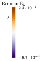
Figure 3: The difference in 𝔼​y\mathbb{E}y computed via the pce[5] and the POD approximation of dimension k’=9 on the base of pce[2].

Motivated by [12, Example 3.1], we consider a stationary convection diffusion problem as in (7) with uncertainty in the conductivity coefficient.

As the geometrical setup, let Ω⊂ℝ3\Omega\subset\mathbb{R}^{3} be a cylindrical domain of radius Ro=1R_{\textsf{o}}=1 without its core of radius Ri=0.4R_{\textsf{i}}=0.4 that is subdivided into 44 subdomains Ωi\Omega_{i}, i=1,2,3,4i=1,2,3,4, as illustrated in Figure 1.

To model the uncertainty in the conductivity coefficient κ\kappa, independently on each subdomain Ωi\Omega_{i}, we assume κ\kappa to be a random variable of a random parameter αi\alpha_{i} via

κ|Ωi=κ¯+αi\kappa\bigl|_{\Omega_{i}}=\bar{\kappa}+\alpha_{i}

where κ¯\bar{\kappa} is a reference value, and write κ⁡(α)\kappa(\alpha) to express the dependence on the random parameter.

In the presented example, we set κ¯=5⋅10−4\bar{\kappa}=5\cdot 10^{-4} and let αi\alpha_{i} be uniformly distributed on

Γi=[−2⋅10−4,2⋅10−4],for i=1,2,3,4.\Gamma_{i}=[-2\cdot 10^{-4},2\cdot 10^{-4}],\quad\text{for }i=1,2,3,4.

As for boundary conditions, we apply zero Dirichlet conditions at the bottom of the domain and zero Neumann conditions elsewhere.

Without particular intentions, the convection bb is chosen as

b⁡(s1,s2,s3)=[(s12+s22−1)​s2−(s12+s22−1)​s1s12​sin⁡(2​s3)]b(s_{1},s_{2},s_{3})=\begin{bmatrix}(s_{1}^{2}+s_{2}^{2}-1)s_{2}\\ -(s_{1}^{2}+s_{2}^{2}-1)s_{1}\\ s_{1}^{2}\sin(2s_{3})\end{bmatrix}

and the inhomogeneity as

f⁡(s1,s2,s3)={−sin⁡(2​π​s1)​sin⁡(4​π​s2)​s3​(0.5−s3),for ​(s1,s2,s3)∈Ω1∪Ω3,0,for ​(s1,s2,s3)∈Ω2∪Ω4;f(s_{1},s_{2},s_{3})=\begin{cases}-\sin(2\pi s_{1})\sin(4\pi s_{2})s_{3}(0.5-s_{3}),&\quad\text{for }(s_{1},s_{2},s_{3})\in\Omega_{1}\cup\Omega_{3},\\ 0,&\quad\text{for }(s_{1},s_{2},s_{3})\in\Omega_{2}\cup\Omega_{4};\end{cases}

see Figure 2 for a snapshot of the solution at κ⁡(0)=κ¯\kappa(0)=\bar{\kappa}.

Moreover, we use C​yCy defined as the spatially averaged value of yy over a concentric annular ring of diameter 0.10.1 that is aligned with the inner boundary at the top surface of the domain; see Figure 1 for the arrangement of the domain of observation.

The values of interest of this numerical study are the expected value 𝔼\mathbb{E} and the variance 𝕍\mathbb{V} of C​yCy that we approximate by a PCE with various levels of refinement.

For the spatial discretization, we use continuous and piecewise linear finite elements on a discretization of the domain by tetrahedra. Although the mesh is refined at the critical parts, namely the edges of the domain and the surfaces where the observation is taken and the Dirichlet condition is applied, we need about 150,000150,000 degrees of freedom for the spatial dimension to have a relative error with respect to the finest considered discretization of less than 10−410^{-4}; see Table 1.

In the experiments we used PCE with the same number of degrees of freedom pcedim for all uncertainty dimensions and write pce[d] to refer to the PCE discretization of dimension dd as well as the expected value/variance of C​yCy based on this discretization. As can be seen in Table 2, for computing the expected value/variance of C​yCy, convergence of the PCE discretization is achieved already for low dimensions. However, although the computations are well parallelized, the computation times for the moderate PCE discretizations are already in the order of days; see Table 2.

Spatial DOFs C​y|κ=4⋅10−4Cy\bigl|_{\kappa=4\cdot 10^{-4}}
56951 1.1165821.116582
72206 1.0774431.077443
90458 1.0693721.069372
127771 1.0697691.069769
154545 1.0658851.065885
192786 1.0659971.065997
237941 1.0646281.064628
Table 1: Computed C​yCy at κ=4⋅10−4\kappa=4\cdot 10^{-4} versus the number of degrees of freedom for the spatial discretization.
pcedim pce[.] runtime [s] difference to pce[5]
2 0.88098230.8809823/0.008972460.00897246 1248.45 −3.9⋅10−5-3.9\cdot 10^{-5}/ −1.0⋅10−4-1.0\cdot 10^{-4}
3 0.88109210.8810921/0.009080180.00908018 7097.21 7.1⋅10−5\phantom{-}7.1\cdot 10^{-5}/9.8⋅10−6\phantom{-}9.8\cdot 10^{-6}
4 0.88101510.8810151/0.009070370.00907037 20059.9 −6.0⋅10−6-6.0\cdot 10^{-6} /−4.2⋅10−7-4.2\cdot 10^{-7}
5 0.88102110.8810211/0.009070790.00907079 49365.4 —
Table 2: The computed expected value/variance of C​yCy based on a PCE discretization, the runtime of its computation, as well as the difference to the value of the finest computed discretization versus the dimension of the PCE.

This gives motivation for the use of the Galerkin POD approach that, as we will prove, is capable to improve the estimate of a coarse PCE discretization by one order of magnitude with little computational overhead.

For that, we use the tensor of coefficients of the pce[2] discretization to compute a basis for the space discretization that is optimal in terms of Theorem 2.3. We set up the reduced models of varying size (which we denote by k’) and compare the computed differences to the expected value/variance of pce[5] for various levels of PCE; see Table 3.

The distribution of the error of the POD approximation of the expected value of the variable yy is plotted in Figure 3.

Note that because PCE(2) leads to 24=162^{4}=16 snapshots, POD dimensions larger than 1616 do not add additional information to the reduced system; cp. also Table 7 where we tabulate the projection error from the POD reduction as defined in (3).

We find that, for the expected value 𝔼​y\mathbb{E}y, with k’=6 the reduced order model recovers the difference between pce[2] and pce[5] and that for k’=15 and k’=16 and a pcedim that exceeds the training data, the approximation error is in the order of finer PCE discretizations with the fine model, which is about 6⋅10−66\cdot 10^{-6}; compare Table 2 and Table 3.

As for the timings, we note that for these small POD dimensions, the effort for computing the POD modes (around 5s) and evaluating the reduced models (around 0.5s) is negligible if compared to the time to compute the data or even the evaluation of pce[5] with the full model; see Table 2.

These results show that with the multidimensional Galerkin-POD reduction, we can use the pce[2] data to compute an approximation to the expected value that is more accurate than pce[4] in just a 1/161/16th of the computational time (about 1253 vs. 20059.9 seconds.)

As for the approximation of the variance 𝕍​C​y\mathbb{V}Cy, the Galerkin-POD reduced model (see Table 4 significantly improves the pce[2] approximation and almost reaches the accuracy of pce[3] in less than 1/5 of the computational time (about 1253 vs. 7097 seconds.)

k’ pce[2] pce[3] pce[4] pce[5]
3 2.99⋅10−42.99\cdot 10^{-4} 2.60⋅10−42.60\cdot 10^{-4} 2.59⋅10−42.59\cdot 10^{-4} 2.59⋅10−42.59\cdot 10^{-4}
6 3.34⋅10−53.34\cdot 10^{-5} 1.05⋅10−61.05\cdot 10^{-6} 1.20⋅10−61.20\cdot 10^{-6} 1.20⋅10−61.20\cdot 10^{-6}
9 3.86⋅10−53.86\cdot 10^{-5} 3.51⋅10−63.51\cdot 10^{-6} 3.29⋅10−63.29\cdot 10^{-6} 3.29⋅10−63.29\cdot 10^{-6}
12 3.88⋅10−53.88\cdot 10^{-5} 1.09⋅10−51.09\cdot 10^{-5} 1.09⋅10−51.09\cdot 10^{-5} 1.09⋅10−51.09\cdot 10^{-5}
15 3.88⋅10−53.88\cdot 10^{-5} 8.27⋅10−68.27\cdot 10^{-6} 8.26⋅10−68.26\cdot 10^{-6} 8.26⋅10−68.26\cdot 10^{-6}
16 3.88⋅10−53.88\cdot 10^{-5} 4.48⋅10−64.48\cdot 10^{-6} 4.36⋅10−64.36\cdot 10^{-6} 4.37⋅10−64.37\cdot 10^{-6}
Table 3: Absolute value of the error in the POD approximation of 𝔼​C​y\mathbb{E}Cy for various POD dimensions of the spatial discretization and various PCE levels. The POD approximation is based on the data of pce[2], i.e. 1616 snapshots located at corresponding quadrature points.
k’ pce[2] pce[3] pce[4] pce[5]
3 2.46⋅10−42.46\cdot 10^{-4} 1.56⋅10−41.56\cdot 10^{-4} 1.55⋅10−41.55\cdot 10^{-4} 1.55⋅10−41.55\cdot 10^{-4}
6 9.72⋅10−59.72\cdot 10^{-5} 9.59⋅10−69.59\cdot 10^{-6} 9.07⋅10−69.07\cdot 10^{-6} 9.07⋅10−69.07\cdot 10^{-6}
9 9.88⋅10−59.88\cdot 10^{-5} 1.23⋅10−51.23\cdot 10^{-5} 1.17⋅10−51.17\cdot 10^{-5} 1.17⋅10−51.17\cdot 10^{-5}
12 9.83⋅10−59.83\cdot 10^{-5} 1.50⋅10−51.50\cdot 10^{-5} 1.46⋅10−51.46\cdot 10^{-5} 1.46⋅10−51.46\cdot 10^{-5}
15 9.83⋅10−59.83\cdot 10^{-5} 1.44⋅10−51.44\cdot 10^{-5} 1.41⋅10−51.41\cdot 10^{-5} 1.41⋅10−51.41\cdot 10^{-5}
16 9.83⋅10−59.83\cdot 10^{-5} 1.33⋅10−51.33\cdot 10^{-5} 1.29⋅10−51.29\cdot 10^{-5} 1.29⋅10−51.29\cdot 10^{-5}
Table 4: Absolute value of the error in the POD approximation of the variance 𝕍​C​y\mathbb{V}Cy for various POD dimensions of the spatial discretization and various PCE levels. The POD approximation is based on the data of pce[2], i.e. 1616 snapshots located at corresponding quadrature points.

To illustrate the fundamental benefit of including the PCE expansion in the POD definition via the product space approach, we investigate the approximation by reduced models based on random snapshots. It turns out that, for the same number of snapshots as with the PCE approach, the approximation errors may reach a similar level but slightly higher level as the snapshots based on the PCE abscissae; see Table 5. However, the randomness in the snapshots makes the approximation unreliable. In fact, the median of 1010 samples gave a worse approximation than the median of 55 samples. In the worse case, the error level is one order of magnitude above the error that is achieved with the same effort via the PCE based reduction 22; see Table 2.

Interestingly, for the approximation of the variance 𝕍​C​y\mathbb{V}Cy, the reduced model based on random snapshots performs as well as the PCE based reduction; see Table 6.

k’ pce[2] pce[3] pce[4] pce[5]
3 1.3⋅10−41.3\cdot 10^{-4}/2.4⋅10−42.4\cdot 10^{-4} 1.9⋅10−41.9\cdot 10^{-4}/2.0⋅10−42.0\cdot 10^{-4} 1.9⋅10−41.9\cdot 10^{-4}/2.0⋅10−42.0\cdot 10^{-4} 1.9⋅10−41.9\cdot 10^{-4}/2.0⋅10−42.0\cdot 10^{-4}
6 2.9⋅10−42.9\cdot 10^{-4}/4.2⋅10−54.2\cdot 10^{-5} 2.3⋅10−42.3\cdot 10^{-4}/9.2⋅10−59.2\cdot 10^{-5} 2.2⋅10−42.2\cdot 10^{-4}/9.2⋅10−59.2\cdot 10^{-5} 2.2⋅10−42.2\cdot 10^{-4}/9.2⋅10−59.2\cdot 10^{-5}
9 8.3⋅10−58.3\cdot 10^{-5}/8.2⋅10−58.2\cdot 10^{-5} 1.3⋅10−41.3\cdot 10^{-4}/1.3⋅10−41.3\cdot 10^{-4} 1.3⋅10−41.3\cdot 10^{-4}/1.5⋅10−41.5\cdot 10^{-4} 1.3⋅10−41.3\cdot 10^{-4}/1.5⋅10−41.5\cdot 10^{-4}
12 9.1⋅10−59.1\cdot 10^{-5}/2.4⋅10−52.4\cdot 10^{-5} 3.3⋅10−53.3\cdot 10^{-5}/5.5⋅10−55.5\cdot 10^{-5} 3.2⋅10−53.2\cdot 10^{-5}/6.2⋅10−56.2\cdot 10^{-5} 3.2⋅10−53.2\cdot 10^{-5}/1.0⋅10−41.0\cdot 10^{-4}
15 1.2⋅10−51.2\cdot 10^{-5}/1.1⋅10−51.1\cdot 10^{-5} 5.3⋅10−65.3\cdot 10^{-6}/5.0⋅10−55.0\cdot 10^{-5} 4.7⋅10−64.7\cdot 10^{-6}/7.0⋅10−57.0\cdot 10^{-5} 4.7⋅10−64.7\cdot 10^{-6}/7.3⋅10−57.3\cdot 10^{-5}
16 2.6⋅10−52.6\cdot 10^{-5}/2.5⋅10−52.5\cdot 10^{-5} 2.5⋅10−52.5\cdot 10^{-5}/4.7⋅10−54.7\cdot 10^{-5} 1.4⋅10−51.4\cdot 10^{-5}/4.3⋅10−54.3\cdot 10^{-5} 7.3⋅10−67.3\cdot 10^{-6}/3.8⋅10−53.8\cdot 10^{-5}
Table 5: Absolute value of the error in the POD approximation of 𝔼α​C​y\mathbb{E}_{\alpha}Cy for various POD dimensions of the spatial discretization based on 1616 random snapshots (median value out of 55/1010 realizations)
k’ pce[2] pce[3] pce[4] pce[5]
3 5.7⋅10−45.7\cdot 10^{-4}/2.9⋅10−52.9\cdot 10^{-5} 6.9⋅10−46.9\cdot 10^{-4}/6.1⋅10−56.1\cdot 10^{-5} 6.9⋅10−46.9\cdot 10^{-4}/6.2⋅10−56.2\cdot 10^{-5} 6.9⋅10−46.9\cdot 10^{-4}/6.2⋅10−56.2\cdot 10^{-5}
6 4.7⋅10−54.7\cdot 10^{-5}/7.7⋅10−57.7\cdot 10^{-5} 1.6⋅10−41.6\cdot 10^{-4}/2.8⋅10−52.8\cdot 10^{-5} 1.6⋅10−41.6\cdot 10^{-4}/2.9⋅10−52.9\cdot 10^{-5} 1.6⋅10−41.6\cdot 10^{-4}/2.9⋅10−52.9\cdot 10^{-5}
9 6.4⋅10−56.4\cdot 10^{-5}/1.0⋅10−41.0\cdot 10^{-4} 3.6⋅10−53.6\cdot 10^{-5}/2.9⋅10−52.9\cdot 10^{-5} 3.7⋅10−53.7\cdot 10^{-5}/2.0⋅10−52.0\cdot 10^{-5} 3.7⋅10−53.7\cdot 10^{-5}/9.7⋅10−69.7\cdot 10^{-6}
12 9.1⋅10−59.1\cdot 10^{-5}/1.0⋅10−41.0\cdot 10^{-4} 9.6⋅10−69.6\cdot 10^{-6}/5.5⋅10−65.5\cdot 10^{-6} 1.0⋅10−51.0\cdot 10^{-5}/1.1⋅10−51.1\cdot 10^{-5} 1.0⋅10−51.0\cdot 10^{-5}/9.8⋅10−69.8\cdot 10^{-6}
15 1.0⋅10−41.0\cdot 10^{-4}/1.1⋅10−41.1\cdot 10^{-4} 1.3⋅10−51.3\cdot 10^{-5}/1.0⋅10−51.0\cdot 10^{-5} 1.3⋅10−51.3\cdot 10^{-5}/1.0⋅10−51.0\cdot 10^{-5} 1.3⋅10−51.3\cdot 10^{-5}/8.9⋅10−68.9\cdot 10^{-6}
16 1.0⋅10−41.0\cdot 10^{-4}/1.0⋅10−41.0\cdot 10^{-4} 1.6⋅10−51.6\cdot 10^{-5}/4.7⋅10−64.7\cdot 10^{-6} 4.1⋅10−54.1\cdot 10^{-5}/1.1⋅10−51.1\cdot 10^{-5} 3.8⋅10−53.8\cdot 10^{-5}/1.3⋅10−51.3\cdot 10^{-5}
Table 6: Absolute value of the error in the POD approximation of the variance 𝕍α​C​y\mathbb{V}_{\alpha}Cy for various POD dimensions of the spatial discretization based on 1616 random snapshots (median value out of 55/1010 realizations)

Thus, we conclude that because of the randomness that is not compensated by an improved performance, a POD based on random snapshots is not well suited to approximate a system with uncertain coefficients.

This is also indicated by the behavior of the projection error that we quantify as follows. If {y⁡(αi)}i=1,…,k\{y(\alpha^{i})\}_{i=1,\dotsc,k} with ai=(α1i,α2i,α3i,α4i)a^{i}=(\alpha_{1}^{i},\alpha_{2}^{i},\alpha_{3}^{i},\alpha_{4}^{i}) is a realization of a set of snapshots, then the corresponding k′k^{\prime} POD modes are the k′k^{\prime} leading left singular vectors of the matrix

𝐋𝒴𝖳​[y⁡(α1)y⁡(α2)⋯​y​(αk)],\mathbf{L}_{\mathcal{Y}}^{\mathsf{T}}\begin{bmatrix}y(\alpha^{1})&y(\alpha^{2})&\dotsm y(\alpha^{k})\end{bmatrix},

where 𝐋𝒴\mathbf{L}_{\mathcal{Y}} is a Cholesky factor of the mass matrix 𝐌𝒴\mathbf{M}_{\mathcal{Y}} of the finite element discretization; cp. Theorem 2.3. Let those singular vectors be the columns of the matrix V𝒴,k′V_{\mathcal{Y},k^{\prime}}. Then the projection of the snapshots reads

𝐋𝒴−𝖳​V𝒴,k′​V𝒴,k′𝖳​𝐋𝒴​[y⁡(α1)y⁡(α2)⋯​y​(αk)]\mathbf{L}_{\mathcal{Y}}^{-{\mathsf{T}}}V_{\mathcal{Y},k^{\prime}}V_{\mathcal{Y},k^{\prime}}^{\mathsf{T}}\mathbf{L}_{\mathcal{Y}}\begin{bmatrix}y(\alpha_{1})&y(\alpha_{2})&\dotsm y(\alpha_{k})\end{bmatrix}

and the projection error in the estimated mean of C​yCy becomes

eC​y;k,k′:=1k​‖C⁡[I−𝐋𝒴−𝖳​V𝒴,k′​V𝒴,k′𝖳​𝐋𝒴]​[y⁡(α1)y⁡(α2)⋯​y​(αk)]‖1.e_{Cy;k,k^{\prime}}:=\frac{1}{k}\|C[I-\mathbf{L}_{\mathcal{Y}}^{-{\mathsf{T}}}V_{\mathcal{Y},k^{\prime}}V_{\mathcal{Y},k^{\prime}}^{\mathsf{T}}\mathbf{L}_{\mathcal{Y}}]\begin{bmatrix}y(\alpha_{1})&y(\alpha_{2})&\dotsm y(\alpha_{k})\end{bmatrix}\|_{1}. (13)

For the case of 1616 random snapshots, unlike the PCE case tabulated in Table 7, the projection error stagnates at the level of 10−1010^{-10} (see Table 8) and only drops down to machine precision for k=k′k=k^{\prime}, where the projection becomes the identity. More random snapshots do not improve this situation; see the lower row of Table 8 where we report the projection errors for 8080 random snapshots. In fact, the reduced models based on 8080 random snapshots did not provide a measurable improvement over the results displayed in Table 5 so that we do not report them here.

All numerical computations were parallelized in 1616 threads and performed on a cluster computing node with 22 Intel Xeon Silver 4110 CPUs with 2.102.10GHz, 2⋅82\cdot 8 virtual cores and 188188GB RAM. The reported timings are the minimum wall time out of 55 runs. The codes that set up, perform, and post process the numerical examples as well as the raw data of the presented cases are available as laid out in Figure 4.

k’ 3 6 9 12 15 16
Projection error 5.1⋅10−65.1\cdot 10^{-6} 3.1⋅10−83.1\cdot 10^{-8} 3⋅10−93\cdot 10^{-9} 9.5⋅10−129.5\cdot 10^{-12} 3⋅10−143\cdot 10^{-14} 2.4⋅10−152.4\cdot 10^{-15}
Table 7: The projection error for varying dimension of the reduced space
k’ 3 6 9 12 15 16
eC​y;16,k′e_{Cy;16,k^{\prime}} 5.96⋅10−65.96\cdot 10^{-6} 1.1⋅10−71.1\cdot 10^{-7} 1.88⋅10−81.88\cdot 10^{-8} 3.99⋅10−93.99\cdot 10^{-9} 2.34⋅10−102.34\cdot 10^{-10} 3.1⋅10−153.1\cdot 10^{-15}
eC​y;80,k′e_{Cy;80,k^{\prime}} 5.94⋅10−65.94\cdot 10^{-6} 8.34⋅10−88.34\cdot 10^{-8} 4.03⋅10−84.03\cdot 10^{-8} 1.37⋅10−81.37\cdot 10^{-8} 8.99⋅10−98.99\cdot 10^{-9} 8.37⋅10−98.37\cdot 10^{-9}
Table 8: The projection error in the estimated mean as defined in (13) for k=16k=16 and k=80k=80 random snapshots and for varying dimension k’ of the reduced space (median values out of 55 realizations).

6 Verification of the Approach

The presented numerical example showed that the proposed Galerkin-POD reduction leads to a significant speedup and memory savings in the PCE approximation.

In order to verify the PCE approach for uncertainty quantification for convection-diffusion problems as considered above, we present two illustrative examples that have similar dynamics but that allow for an analytic expression of the expected values and variances as well as for extensive Monte Carlo simulations for comparison.

The examples are motivated by the observation that for b=0b=0 in (7), the solution yy to the discrete problem is given as

y⁡(α)=𝐀α−1​fy(\alpha)=\mathbf{A}_{\alpha}^{-1}f (14)

where 𝐀α\mathbf{A}_{\alpha} is the discrete Laplacian and ff is the right hand side. For this problem and a given observation operator CC, the expected value of C​yCy is given as

∫ΓC​𝐀α−1​f​ d​ℙα\int_{\Gamma}C\mathbf{A}_{\alpha}^{-1}f\text{~{d}}\mathbb{P}_{\alpha}

For the first example, we mimick the situation that the diffusion coefficient is constant in space and dependent on a univariate distribution so that 𝐀α=α1​𝐀\mathbf{A}_{\alpha}=\alpha_{1}\mathbf{A} and so that, for the solution y1​(α1)=1α1​𝐀α−1​fy_{1}(\alpha_{1})=\frac{1}{\alpha_{1}}\mathbf{A}_{\alpha}^{-1}f, the expected value reads

𝔼​y1=∫ΓC​𝐀α−1​f​ d​ℙα=C​∫Γ11α1​ d​ℙα1​𝐀−1​f,\mathbb{E}y_{1}=\int_{\Gamma}C\mathbf{A}_{\alpha}^{-1}f\text{~{d}}\mathbb{P}_{\alpha}=C\int_{\Gamma_{1}}\frac{1}{\alpha_{1}}\text{~{d}}\mathbb{P}_{\alpha_{1}}\mathbf{A}^{-1}f,

which, for α1\alpha_{1} being uniformly distributed on Γ1=[α¯1,α¯1]\Gamma_{1}=[\underline{\alpha}_{1},\overline{\alpha}_{1}], becomes

𝔼​y1=1α¯1−α¯1​∫α¯1α¯11α​ d​α​C​𝐀−1​f.\mathbb{E}y_{1}=\frac{1}{\overline{\alpha}_{1}-\underline{\alpha}_{1}}\int^{\overline{\alpha}_{1}}_{\underline{\alpha}_{1}}\frac{1}{\alpha}\text{~{d}}\alpha C\mathbf{A}^{-1}f.

With the same arguments, the variance can be computed as

𝕍​y1=1α¯1−α¯1​∫α¯1α¯11α2​ d​α​(C​𝐀−1​f)2−𝔼​y12.\mathbb{V}y_{1}=\frac{1}{\overline{\alpha}_{1}-\underline{\alpha}_{1}}\int^{\overline{\alpha}_{1}}_{\underline{\alpha}_{1}}\frac{1}{\alpha^{2}}\text{~{d}}\alpha(C\mathbf{A}^{-1}f)^{2}-\mathbb{E}y_{1}^{2}.

Since CC, 𝐀−1\mathbf{A}^{-1}, and ff are but constant factors, we can set them to 11 and the expected performance of PCE or Monte Carlo for such a case can be analyzed by their performance in the numerical integration of the integral

𝔼​y1=1α¯1−α¯1​∫α¯1α¯11α​ d​αor𝕍​y1=1α¯1−α¯1​∫α¯1α¯11α2​ d​α−𝔼​y12.\mathbb{E}y_{1}=\frac{1}{\overline{\alpha}_{1}-\underline{\alpha}_{1}}\int^{\overline{\alpha}_{1}}_{\underline{\alpha}_{1}}\frac{1}{\alpha}\text{~{d}}\alpha\quad\text{or}\quad\mathbb{V}y_{1}=\frac{1}{\overline{\alpha}_{1}-\underline{\alpha}_{1}}\int^{\overline{\alpha}_{1}}_{\underline{\alpha}_{1}}\frac{1}{\alpha^{2}}\text{~{d}}\alpha-\mathbb{E}y_{1}^{2}. (15)

For the second example, we set

α=(α1,α2),𝐀α=[α1ϵϵα2],f=[11],C=[11]\alpha=(\alpha_{1},\alpha_{2}),\quad\mathbf{A}_{\alpha}=\begin{bmatrix}\alpha_{1}&\epsilon\\ \epsilon&\alpha_{2}\end{bmatrix},\quad f=\begin{bmatrix}1\\ 1\end{bmatrix},\quad C=\begin{bmatrix}1&1\end{bmatrix}

so that, with α1\alpha_{1} as above and α2\alpha_{2} being distributed uniformly on Γ2=[α¯2,α¯2]\Gamma_{2}=[\underline{\alpha}_{2},\overline{\alpha}_{2}], the expected value and the variance for the corresponding solution y2​(α1,α2)y_{2}(\alpha_{1},\alpha_{2}) read

𝔼​y2=1α¯1−α¯11α¯2−α¯2∫α¯1α¯1∫α¯2α¯21α1​α2−ϵ2(α1+α2−2ϵ) dα2 dα1and𝕍​y2=1α¯1−α¯1​1α¯2−α¯2​∫α¯1α¯1∫α¯2α¯2[1α1​α2−ϵ2​(α1+α2−2​ϵ)]2​ d​α2​ d​α1−(𝔼​y2)2.\begin{split}\mathbb{E}y_{2}&=\frac{1}{\overline{\alpha}_{1}-\underline{\alpha}_{1}}\frac{1}{\overline{\alpha}_{2}-\underline{\alpha}_{2}}\int^{\overline{\alpha}_{1}}_{\underline{\alpha}_{1}}\int^{\overline{\alpha}_{2}}_{\underline{\alpha}_{2}}\frac{1}{\alpha_{1}\alpha_{2}-\epsilon^{2}}(\alpha_{1}+\alpha_{2}-2\epsilon)\text{~{d}}\alpha_{2}\text{~{d}}\alpha_{1}\quad\text{and}\\ \mathbb{V}y_{2}&=\frac{1}{\overline{\alpha}_{1}-\underline{\alpha}_{1}}\frac{1}{\overline{\alpha}_{2}-\underline{\alpha}_{2}}\int^{\overline{\alpha}_{1}}_{\underline{\alpha}_{1}}\int^{\overline{\alpha}_{2}}_{\underline{\alpha}_{2}}\biggl[\frac{1}{\alpha_{1}\alpha_{2}-\epsilon^{2}}(\alpha_{1}+\alpha_{2}-2\epsilon)\biggr]^{2}\text{~{d}}\alpha_{2}\text{~{d}}\alpha_{1}-(\mathbb{E}y_{2})^{2}.\end{split} (16)

This example simulates the case of a diffusion process with two compartments with different random diffusion parameters and with a constant ϵ\epsilon as the parameter of the coupling.

For the two examples (15) and (16), we use the parameters

α¯1=α¯2=3⋅10−4,α¯1=α¯2=7⋅10−4,ϵ=1⋅10−4\underline{\alpha}_{1}=\underline{\alpha}_{2}=3\cdot 10^{-4},\quad\overline{\alpha}_{1}=\overline{\alpha}_{2}=7\cdot 10^{-4},\quad\epsilon=1\cdot 10^{-4}

and compute the reference values for the means and variances

𝔼​y1=2118.24465097,𝕍​y1=274944.360550,𝔼​y2=3504.22709343,𝕍​y2=261037.034256,\mathbb{E}y_{1}=2118.24465097,\quad\mathbb{V}y_{1}=274944.360550,\quad\mathbb{E}y_{2}=3504.22709343,\quad\mathbb{V}y_{2}=261037.034256,

via evaluating the integrals with the help of a computer algebra package.

With the reference values at hand, we can estimate the approximation quality of the PCE and MC simulations. The PCE simulation provides stable and quickly converging approximations of the expected values and variances for the example problems; see Table 9 and Table 11. Opposed to that, plain Monte Carlo simulations, show very slow convergence; see Table 10 and Table 12. In fact, for example, for estimating the expected value 𝔼​y2\mathbb{E}y_{2} up to a relative error in the order of 10−510^{-5}, it takes 1,000,0001,000,000 Monte Carlo simulations or 1616 simulations for the pce[4] approximation.

Since the numerical example of Section 5 has a similar structure as the two illustrative examples of this section, we conclude that the proposed PCE discretization is well suited for this kind of multivariate uncertainty quantification. Also, we note that a plain Monte Carlo simulation for verification purposes is infeasible in the large-scale setup as in Section 5, where one single forward simulation lasts about one minute.

Method pce[3] pce[4] pce[5] pce[6]
Relative error for 𝔼​y1\mathbb{E}y_{1} −1.18⋅10−4-1.18\cdot 10^{-4} −5.24⋅10−6-5.24\cdot 10^{-6} −2.31⋅10−7-2.31\cdot 10^{-7} −1.01⋅10−8-1.01\cdot 10^{-8}
Relative error for 𝕍​y1\mathbb{V}y_{1} −1.00⋅10−2-1.00\cdot 10^{-2} −6.21⋅10−4-6.21\cdot 10^{-4} −3.51⋅10−5-3.51\cdot 10^{-5} −1.88⋅10−6-1.88\cdot 10^{-6}
Table 9: Approximation errors for the 1D problem (15) with PCE discretizations pce[N] with N degrees of freedom in the uncertainty dimension.
Method mc[10,000] mc[100,000] mc[1,000,000]
Relative error for 𝔼​y1\mathbb{E}y_{1} 4.01⋅10−4\phantom{-}4.01\cdot 10^{-4} −1.37⋅10−4-1.37\cdot 10^{-4} −9.35⋅10−5-9.35\cdot 10^{-5}
Relative error for 𝕍​y1\mathbb{V}y_{1} 2.36⋅10−3\phantom{-}2.36\cdot 10^{-3} 1.82⋅10−3\phantom{-}1.82\cdot 10^{-3} 4.21⋅10−4\phantom{-}4.21\cdot 10^{-4}
Table 10: Approximation errors for the 1D problem (15) with Monte Carlo simulations mc[N] with N simulations. (Median value out of 15 realizations).
Method pce[3] pce[4] pce[5] pce[6]
Relative error for 𝔼​y2\mathbb{E}y_{2} −1.23⋅10−4-1.23\cdot 10^{-4} −6.01⋅10−6-6.01\cdot 10^{-6} −2.91⋅10−7-2.91\cdot 10^{-7} −1.41⋅10−8-1.41\cdot 10^{-8}
Relative error for 𝕍​y2\mathbb{V}y_{2} −1.20⋅10−2-1.20\cdot 10^{-2} −8.16⋅10−4-8.16\cdot 10^{-4} −5.07⋅10−5-5.07\cdot 10^{-5} −2.98⋅10−6-2.98\cdot 10^{-6}
Table 11: Approximation errors for the 2D problem (16) with PCE discretizations pce[N] with N degrees of freedom in every uncertainty dimension.
Method mc[10,000] mc[100,000] mc[1,000,000]
Relative error for 𝔼​y2\mathbb{E}y_{2} 7.09⋅10−4\phantom{-}7.09\cdot 10^{-4} 1.11⋅10−4\phantom{-}1.11\cdot 10^{-4} −3.71⋅10−5-3.71\cdot 10^{-5}
Relative error for 𝕍​y2\mathbb{V}y_{2} −4.75⋅10−3-4.75\cdot 10^{-3} −3.61⋅10−4-3.61\cdot 10^{-4} −3.74⋅10−4-3.74\cdot 10^{-4}
Table 12: Approximation errors for the 2D problem (16) with Monte Carlo simulations mc[N] with N simulations. (Median value out of 11 realizations).

7 Conclusion

The theory of multidimensional Galerkin POD naturally applies to problems with multivariate uncertainties and can be made tractable for numerical experiments by exploiting the underlying tensor structures. The multidimensional POD that includes Polynomial Chaos Expansions of the candidate solutions lead to a significant efficiency gain in the uncertainty quantification as we have illustrated in a linear convection diffusion example. For comparison, the direct POD approach based on random snapshots is somewhat inconclusive. In a few setups, it well competes with the PCE based reduction but, generally, the approximation is worse and without showing reliable trends that can be used for finding preferable configurations of number of snapshots and dimensions of the reduced order model. Future work will include the investigation of POD reduction also for the PCE dimensions and the inclusion of these reduced models for optimal control of uncertain systems.

Code and Data Availability

The source code of the implementations used to compute the presented results is available from:

doi:10.5281/zenodo.4005724

github.com/mpimd-csc/multidim-genpod-uq

under the MIT license and is authored by Jan Heiland.

Figure 4: Link to code and data.

References

  • [1] M. Arnst, R. Ghanem, E. Phipps, and J. Red-Horse. Reduced chaos expansions with random coefficients in reduced-dimensional stochastic modeling of coupled problems. Int. J. Numer. Methods Eng., 97(5):352–376, 2014. doi:10.1002/nme.4595.
  • [2] C. Audouze and P. B. Nair. Galerkin reduced-order modeling scheme for time-dependent randomly parametrized linear partial differential equations. Int. J. Numer. Methods Eng., 92(4):370–398, 2012. doi:10.1002/nme.4341.
  • [3] J. Ballani and L. Grasedyck. Hierarchical tensor approximation of output quantities of parameter-dependent PDEs. SIAM/ASA J. Uncertain. Quantif., 3(1):852–872, 2015. doi:10.1137/140960980.
  • [4] M. Baumann, P. Benner, and J. Heiland. Space-time Galerkin POD with application in optimal control of semi-linear parabolic partial differential equations. SIAM J. Sci. Comput., 40(3):A1611–A1641, 2018. doi:10.1137/17M1135281.
  • [5] M. Baumann, J. Heiland, and M. Schmidt. Discrete input/output maps and their relation to Proper Orthogonal Decomposition. In P. Benner, M. Bollhöfer, D. Kressner, C. Mehl, and T. Stykel, editors, Numerical Algebra, Matrix Theory, Differential-Algebraic Equations and Control Theory, pages 585–608. Springer International Publishing, 2015. doi:10.1007/978-3-319-15260-8_21.
  • [6] P. Benner, A. Onwunta, and M. Stoll. Low-rank solution of unsteady diffusion equations with stochastic coefficients. SIAM/ASA J. Uncertain. Quantif., 3(1):622–649, 2015. doi:10.1137/130937251.
  • [7] I. Bianchini, R. Argiento, F. Auricchio, and E. Lanzarone. Efficient uncertainty quantification in stochastic finite element analysis based on functional principal components. Comput. Mech., 56(3):533–549, 2015. doi:10.1007/s00466-015-1185-7.
  • [8] K. A. Cliffe, M. B. Giles, R. Scheichl, and A. L. Teckentrup. Multilevel Monte Carlo methods and applications to elliptic PDEs with random coefficients. Computing and Visualization in Science, 14(1):3–15, 2011. doi:10.1007/s00791-011-0160-x.
  • [9] L. De Lathauwer, B. De Moor, and J. Vandewalle. A multilinear singular value decomposition. SIAM J. Matrix Anal. Appl., 21(4):1253–1278, 2000. doi:10.1137/S0895479896305696.
  • [10] A. D. Fernandes and W. R. Atchley. Gaussian quadrature formulae for arbitrary positive measures. Evolutionary bioinformatics online, 2:251–259, February 2007. URL: http://europepmc.org/articles/PMC2674649.
  • [11] J. Garcke. Sparse grids in a nutshell. In J. Garcke and M. Griebel, editors, Sparse Grids and Applications, pages 57–80, Berlin, Heidelberg, 2013. Springer Berlin Heidelberg. doi:10.1007/978-3-642-31703-3_3.
  • [12] S. Garreis and M. Ulbrich. Constrained optimization with low-rank tensors and applications to parametric problems with PDEs. SIAM J. Sci. Comput., 39(1):A25–A54, 2017. doi:10.1137/16M1057607.
  • [13] A.-L. Haji-Ali, F. Nobile, L. Tamellini, and R. Tempone. Multi-index stochastic collocation for random PDEs. Comput. Methods Appl. Mech. Eng., 306:95–122, 2016. doi:10.1016/j.cma.2016.03.029.
  • [14] B. N. Khoromskij. Tensor numerical methods for multidimensional PDEs: Theoretical analysis and initial applications. ESAIM: Proceedings, 48:1–28, 2015. doi:10.1051/proc/201448001.
  • [15] B. N. Khoromskij and C. Schwab. Tensor-structured Galerkin approximation of parametric and stochastic elliptic PDEs. SIAM J. Sci. Comput., 33(1):364–385, 2011. doi:10.1137/100785715.
  • [16] A. Nouy. Proper generalized decompositions and separated representations for the numerical solution of high dimensional stochastic problems. Arch. Comput. Methods Eng., 17(4):403–434, 2010. doi:10.1007/s11831-010-9054-1.
  • [17] C. W. Rowley. Model reduction for fluids, using balanced Proper Orthogonal Decomposition. Internat. J. Bifur. Chaos Appl. Sci. Engrg., 15(03):997–1013, 2005. doi:10.1142/s0218127405012429.
  • [18] C. Soize. Brief overview of stochastic solvers for the propagation of uncertainties. In Uncertainty Quantification: An Accelerated Course with Advanced Applications in Computational Engineering, pages 133–139. Springer International Publishing, Cham, 2017. doi:10.1007/978-3-319-54339-0_6.
  • [19] L. Tamellini, O. L. Maître, and A. Nouy. Model reduction based on Proper Generalized Decomposition for the stochastic steady incompressible Navier–Stokes equations. SIAM J. Sci. Comput., 36(3), 2014. doi:10.1137/120878999.
  • [20] E. Ullmann. A Kronecker product preconditioner for stochastic Galerkin finite element discretizations. SIAM J. Sci. Comput., 32(2):923–946, 2010. doi:10.1137/080742853.