跳到论文正文
W Papers独立论文阅读器 arXiv:2009.01002 论文正文 计算阅读时间 · 0%
引用这篇论文根据当前论文元数据生成,正式投稿前建议核对。


License: arXiv.org perpetual non-exclusive license
arXiv:2009.01002v6 [cond-mat.supr-con] 22 Oct 2021

A quantum model for rf-SQUIDs based metamaterials enabling 3WM and 4WM Traveling Wave Parametric Amplification

Angelo Greco Affiliation: INRiM, Istituto Nazionale di Ricerca Metrologica, Strada delle Cacce 91, 10135 Torino, Italy Affiliation: Department of Electronics and Telecommunications, PoliTo, Corso Castelfidardo 39, 10129 Torino, Italy    Luca Fasolo Affiliation: INRiM, Istituto Nazionale di Ricerca Metrologica, Strada delle Cacce 91, 10135 Torino, Italy Affiliation: Department of Electronics and Telecommunications, PoliTo, Corso Castelfidardo 39, 10129 Torino, Italy    Alice Meda, Luca Callegaro Affiliation: INRiM, Istituto Nazionale di Ricerca Metrologica, Strada delle Cacce 91, 10135 Torino, Italy    Emanuele Enrico Email: Corresponding author: e.enrico@inrim.it Affiliation: INRiM, Istituto Nazionale di Ricerca Metrologica, Strada delle Cacce 91, 10135 Torino, Italy Affiliation: INFN, Trento Institute for Fundamental Physics and Applications, I-38123, Povo, Trento, Italy
August 11, 2026
Abstract

A quantum model for Josephson-based metamaterials working in the Three-Wave Mixing (3WM) and Four-Wave Mixing (4WM) regimes at the single-photon level is presented. The transmission line taken into account, namely Josephson Traveling Wave Parametric Amplifier (JTWPA), is a bipole composed of a chain of rf-SQUIDs which can be biased by a DC current or a magnetic field to activate the 3WM or 4WM nonlinearities. The model exploits a Hamiltonian approach to analytically determine the time evolution of the system both in the Heisenberg and interaction pictures. The former returns the analytic form of the gain of the amplifier, while the latter allows recovering the probability distributions vs. time of the photonic populations, for multimodal Fock and coherent input states. The dependence of the metamaterial’s nonlinearities is presented in terms of circuit parameters in a lumped model framework while evaluating the effects of the experimental conditions on the model validity.

I Introduction

Superconducting amplifiers are nowadays widely used for the manipulation of single photons in several ranges of the electromagnetic spectrum. From microwaves to X-rays these devices have shown unrivalled performances for what concerns quantum efficiency, resolving power and added noise, compared to their solid-state counterparts Hadfield 2009; Natarajan et al. 2012; Ullom et al. 2014; Fukuda et al. 2011; Miller et al. 2003; Lita et al. 2008. The peculiar characteristics of superconducting materials allow engineering highly performing resonators and cavities, characterised by a quality factor of the order of ≈1010\approx 10^{10} Yang and Deng 2020; Malnou et al. 2018; Castellanos-Beltran et al. 2009; Eichler and Wallraff 2014. Indeed, resonator-based superconducting amplifiers show a quite high gain, in the range of 20 dB20\text{\,}\mathrm{dB} Castellanos-Beltran et al. 2009; however, they are subjected to limited bandwidth making them unsuitable for the multiplexing required in complex systems.
Josephson Traveling Waves Parametric Amplifiers (JTWPAs) and Kinetic Inductance Traveling Wave Amplifiers (KITs) promise to be appropriate devices for this aim in the microwave regime, showing in principle valuable multiplexing capabilities due to their wide bandwidth White et al. 2015. Indeed, it has been shown how the Four-Wave Mixing (4WM) induced in all the Kerr-like media allows amplifying very tiny signals over several GHz\mathrm{GHz} bandwidths with a nearly quantum-limited noise White et al. 2015; Macklin et al. 2015; Zobrist et al. 2019; Chaudhuri et al. 2017. Nevertheless, recent papers show that enabling the Three-Wave Mixing (3WM) interaction, through the introduction of a quadratic nonlinearity in the medium, could provide several benefits and experimental simplifications for what concerns feasibility and integration capabilities. In particular, a three-wave mixer generally requires a lower input pump power, easier output filtering and shows a higher dynamic range Vissers et al. 2016; Zorin 2016; Zorin et al. 2017. These distinctive characteristics make JTWPAs working in 3WM excellent candidates for the readout of quantum-limited detectors (e.g., rf-SETs, rf-SQUIDs), by preserving the quantum properties of their outputs Buehler et al. 2005; Aassime et al. 2001; Henderson et al. 2018. Moreover, a three-wave mixer can be a promising candidate for the generation of heralded photons pairs, since it naturally enables Parametric Down Conversion (PDC) Guo et al. 2017.
In this framework, we develop a quantum model, based on previous theoretical works van der Reep 2019; Arne L. Grimsmo 2017, for a recently proposed JTWPA concept Zorin 2016 covering both the 3WM and 4WM regimes. Previous classical descriptions in terms of electromagnetic waves Zorin 2016; Zorin et al. 2017 were limited to the high power range, completely neglecting any description of the light-matter interaction at the single photon level. Our theory exploits circuit-QED techniques to model a JTWPA made up of a chain of rf-SQUIDs capacitively shunted to ground. The proposed layout can be biased by a DC current or an externally applied magnetic field to activate 3WM or 4WM of the microwave traveling modes. The quantum description allows to analytically treat important figures of merit of the amplifier as the gain, squeezing and the time evolution of arbitrary quantum states at the single-photon level.
The main results of the paper are reported in Section II. In particular, Subsection II.1 reports the Hamiltonian in first quantization formalism, based on the circuit model of a nonlinear lossless transmission line. Then, Subsection II.2 is dedicated to developing the theory through the occupation number formalism, and a 3WM/4WM Hamiltonian is found. A selection of modes follows in Subsection II.3, leading to model the 3WM/4WM quantum mechanical phenomena in the Heisenberg picture. Solving the dynamics of the system (i.e., Langevin equations) allows to analytically calculate the gain, noise figures and squeezing capabilities of the amplifier. In Subsection II.4 the time evolution of Fock and coherent input states due to nonlinear interactions is analytically treated and on these bases various examples of photon statistics in the Fock space are calculated.

II Results

II.1 Hamiltonian of a rf-SQUIDs array embedded in a transmission line

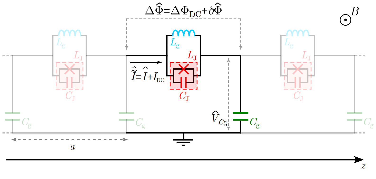
The JTWPA recently proposed Zorin 2016 and theoretically quantum mechanically treated in this paper can be modelled as an array of rf-SQUIDs embedded in a superconducting transmission line. In the following, the Hamiltonian of the system will be derived as a function of its circuit parameters. As represented in Figure 1, each elementary cell is composed by a superconducting loop containing a Josephson junction (with its associated capacitance CJC_{\mathrm{J}} and inductance LJL_{\mathrm{J}}) and a geometrical inductance LgL_{\mathrm{g}}. Furthermore, each loop is coupled to ground through a capacitor CgC_{\mathrm{g}}. The system taken into account is non-dissipative and, for the sake of simplicity, all the elementary cells are considered identical. The length of the elementary cell along the zz-direction (i.e., the propagating direction of the modes) is defined as aa.
In presence of an electromagnetic field, each of these cells stores a certain amount of energy that can be expressed as a function of the conjugate coordinates Φ^\hat{\Phi} and Q^\hat{Q}, the generalized magnetic flux and charge at a certain node respectively, obeying to the commutation relation [Φ^,Q^]=i​ℏ[\hat{\Phi},\hat{Q}]=i\hbar. The total amount of energy can be computed as the sum of the energy stored in each of its components (see Supplemental S-III). Moreover, being the system under analysis a repetition of identical elementary units, the total energy stored in the whole medium can be expressed as the sum of the energy stored in each cell.
Under the assumption that the differences between the Φ^\hat{\Phi} (and Q^\hat{Q}) of a couple of consecutive nodes are small enough, these operators can be considered as functions of both time and space (i.e., Φ^​(z,t)\hat{\Phi}(z,t) and Q^​(z,t)\hat{Q}(z,t)). We then define the flux difference between two subsequent nodes as

Δ​Φ^​(z,t)=Φ^​(z+a,t)−Φ^​(z,t)\displaystyle\Delta\hat{\Phi}(z,t)=\hat{\Phi}(z+a,t)-\hat{\Phi}(z,t) (1)

We can define the Hamiltonian of the system like the sum of the energies stored in every single cell of the device. The circuit elements which appear are discrete, so every cell has its own ground capacitor, Josehpson capacitor, geometrical inductance and Josephson junction. The sum runs over the index nn which labels all the cells.

H^\displaystyle\hat{H} =\displaystyle= ∑n=1NH^n\displaystyle\sum_{n=1}^{N}\hat{H}_{\mathrm{n}} (2a)
=\displaystyle= ∑n=1N(H^Lg+H^Lj+H^Cj+H^Cg)\displaystyle\sum_{n=1}^{N}\left(\hat{H}_{\mathrm{{L_{g}}}}+\hat{H}_{\mathrm{{L_{j}}}}+\hat{H}_{\mathrm{{C_{j}}}}+\hat{H}_{\mathrm{{C_{g}}}}\right) (2b)
=\displaystyle= ∑n=1N(12​Lg​Δ​Φ^​(n​a,t)2+φ0​Ic​(1−cos⁡(Δ​Φ^​(n​a,t)φ0))+CJ2​(∂Δ​Φ^​(n​a,t)∂t)2+12​Cg​Q^​(n​a,t)2)\displaystyle\sum_{n=1}^{N}\left(\frac{1}{2L_{\mathrm{g}}}\Delta\hat{\Phi}(na,t)^{2}+\varphi_{0}I_{\mathrm{c}}\left(1-\cos{\left(\frac{\Delta\hat{\Phi}(na,t)}{\varphi_{0}}\right)}\right)+\frac{C_{\mathrm{J}}}{2}\left(\frac{\partial\Delta\hat{\Phi}(na,t)}{\partial t}\right)^{2}+\frac{1}{2C_{\mathrm{g}}}\hat{Q}(na,t)^{2}\right) (2c)

where in the right-hand side of equation (2b) one can recognize respectively the energy associated to the geometrical inductance LgL_{\mathrm{g}}, the Josephson inductance LJL_{\mathrm{J}}, the Josephson capacitance CJC_{\mathrm{J}} and the ground capacitance CgC_{\mathrm{g}}. NN is the number of unit cells composing the transmission line, IcI_{\mathrm{c}} is the critical current of the Josephson junction and φ0=Φ0/2​π=ℏ/2​e\varphi_{0}=\Phi_{0}/2\pi=\hbar/2e is the reduced flux quantum.
As can be seen, the flux difference function Δ​Φ^​(z,t)\Delta\hat{\Phi}(z,t) is defined for every zz but is calculated at discrete points in correspondence to the multiple integers a​nan of the unit cell length aa. In order to compute the Hamiltonian we can switch from a discrete sum to an approximated continuous sum substituting the summation sign with an integral Loudon 2000, adding the scale factor aa (length of a unit cell), which turns the discrete components in components per unit length. The integration upper limit is the length of the amplifier l=N​al=Na, where NN is the number of unit cells.

H^\displaystyle\hat{H} =∫0l(12​Lg​Δ​Φ^​(z,t)2+φ0​Ic​(1−cos⁡(Δ​Φ^​(z,t)φ0))+CJ2​(∂Δ​Φ^​(z,t)∂t)2+12​Cg​Q^​(z,t)2)​d​za\displaystyle=\int_{0}^{l}\left(\frac{1}{2L_{\mathrm{g}}}\Delta\hat{\Phi}(z,t)^{2}+\varphi_{0}I_{\mathrm{c}}\left(1-\cos{\left(\frac{\Delta\hat{\Phi}(z,t)}{\varphi_{0}}\right)}\right)+\frac{C_{\mathrm{J}}}{2}\left(\frac{\partial\Delta\hat{\Phi}(z,t)}{\partial t}\right)^{2}+\frac{1}{2C_{\mathrm{g}}}\hat{Q}(z,t)^{2}\right)\frac{dz}{a} (3)

The integral can be considered as an approximation of the discrete sum in Equation (2c), where the flux difference across two subsequent cells is to be considered due to the presence of a finite number of Josephson junctions, for which the energy is defined in relation with the flux difference across them.
The presence of an external magnetic field or a DC current through the line induces a constant component in the flux difference across a cell. This means that Δ​Φ^​(z,t)\Delta\hat{\Phi}(z,t) can be considered as the sum of two components, a constant one Δ​ΦDC\Delta{\Phi}_{\mathrm{DC}} and a time-dependent one δ​Φ^​(z,t)\delta\hat{\Phi}(z,t)

Δ​Φ^​(z,t)=Δ​ΦDC+δ​Φ^​(z,t)\Delta\hat{\Phi}(z,t)=\Delta{\Phi}_{\mathrm{DC}}+\delta\hat{\Phi}(z,t) (4)
Refer to caption
Figure 1: Electrical equivalent of a repetition of three elementary cells (periodicity aa) of the rf-SQUIDs based JTWPA. Each cell consists of a superconducting loop containing a geometrical inductance LgL_{\mathrm{g}}, a Josephson junction, with an associated capacitance CJC_{\mathrm{J}} and inductance LJL_{\mathrm{J}}, and a ground capacitor CgC_{\mathrm{g}}. The series can be biased both through an external DC magnetic field BB and a flowing current IDCI_{\mathrm{DC}}. Δ​Φ^\Delta\hat{\Phi} is the magnetic flux difference across the nodes of a cell, while V^Cg\hat{V}_{C_{\mathrm{g}}} is the voltage drop across the ground capacitor.

II.2 Second quantization framework

Here the Hamiltonian will be expressed in terms of ladder operators. In this view, the voltage drop on the ground capacitors CgC_{\mathrm{g}} can be expressed using a mode decomposition assuming that sinusoidal waves are passing through the line (Vool and Devoret 2017)

V^Cg(z,t)=∑nℏ​ωn2​Cg​N(a^nei⁡(kn​z−ωn​t)+H.c.)\hat{V}_{C_{\mathrm{g}}}(z,t)=\sum_{n}\sqrt{\frac{\hbar\omega_{n}}{2C_{\mathrm{g}}N}}\left(\hat{a}_{n}e^{i(k_{n}z-\omega_{n}t)}+\mathrm{H.c.}\right) (5)

where ωn\omega_{n} and knk_{n} are the angular frequency and wavenumber of the nn-th mode while a^n\hat{a}_{n} is its annihilation operator of the nn-th mode. Positive indexes denote progressive waves (kn>0k_{n}>0 and ωn>0\omega_{n}>0), while negative indexes denote regressive waves (k−n=−kn<0k_{-n}=-k_{n}<0 and ω−n=ωn\omega_{-n}=\omega_{n}).
It is trivial to recover the link between the voltage drop and the current passing through a cell given by the classical Telegrapher’s equation, which exploits the inductance of the cell for the nn-th mode LnL_{n}

∂Vn∂z=−Lna​∂In∂t\frac{\partial V_{n}}{\partial z}=-\frac{L_{n}}{a}\frac{\partial I_{n}}{\partial t} (6)

LnL_{n} can be calculated as the parallel between the effective inductance Leff,nL_{\mathrm{eff},n} (composed by the Josephson capacitance CJC_{\mathrm{J}} and the geometrical inductance LgL_{\mathrm{g}}, see Supplemental S-IV) and the Josephson inductance LJL_{\mathrm{J}}. Exploiting the constitutive relation for a generic inductor it can be written that Δ​Φ=L⋅I\Delta{\Phi}=L\cdot I. Hence, using the flux-current relation of a Josephson junction, IJ=Ic​sin⁡(Δ​Φ/φ0)I_{\mathrm{J}}=I_{\mathrm{c}}\sin{\left(\Delta\Phi/\varphi_{0}\right)}, the Josephson inductance LJL_{\mathrm{J}} can be simply expressed, via a nonlinear relation with Δ​Φ\Delta\Phi, as

LJ=Δ​ΦIJ=φ0Ic​Δ​Φ/φ0sin⁡(Δ​Φ/φ0)≡LJ0​Δ​Φ/φ0sin⁡(Δ​Φ/φ0)L_{\mathrm{J}}=\frac{\Delta\Phi}{I_{\mathrm{J}}}=\frac{\varphi_{0}}{I_{\mathrm{c}}}\frac{\Delta\Phi/\varphi_{0}}{\sin{\left(\Delta\Phi/\varphi_{0}\right)}}\equiv L_{\mathrm{J}_{0}}\frac{\Delta\Phi/\varphi_{0}}{\sin{\left(\Delta\Phi/\varphi_{0}\right)}} (7)

with LJ0=φ0/IcL_{\mathrm{J}_{0}}=\varphi_{0}/I_{\mathrm{c}}. It follows that the cell inductance LnL_{n} can be written as

Ln\displaystyle L_{n} =Λn​Lg1+Λn​LgLJ0​sin⁡(Δ​Φ/φ0)(Δ​Φ/φ0)\displaystyle=\frac{\Lambda_{n}L_{\mathrm{g}}}{1+\Lambda_{n}\frac{L_{\mathrm{g}}}{L_{\mathrm{J}_{0}}}\frac{\sin{\left(\Delta\Phi/\varphi_{0}\right)}}{\left(\Delta\Phi/\varphi_{0}\right)}} (8)

where the dispersion coefficient of the nn-th node Λn=1/(1−ωn2​Lg​CJ)\Lambda_{n}=1/(1-\omega_{n}^{2}L_{\text{g}}C_{\text{J}}) (Supplemental S-IV) has been defined. The time-dependent component of equation (4) can be found exploiting the mode decomposition for the AC current through the cell InI_{n} and the inductance LnL_{n} for the corresponding mode as

δ​Φ=∑nLn​In\delta\Phi=\sum_{n}L_{n}I_{n} (9)

Replacing the classical variables by corresponding operator, and accordingly to the standard quantum description of electrical circuits Vool and Devoret 2017, it follows that (see Supplemental S-V)

δ​Φ^=∑n[(1+Λn​LgLJ0​sin⁡(Δ​ΦDC+δ​Φ^φ0)Δ​ΦDC+δ​Φ^φ0)−12​δ​Φ^n(0)]\delta\hat{\Phi}=\sum_{n}\left[\left(1+\Lambda_{n}\frac{L_{\mathrm{g}}}{L_{\mathrm{J}_{0}}}\frac{\sin{\left(\frac{\Delta\Phi_{\mathrm{DC}}+\delta\hat{\Phi}}{\varphi_{0}}\right)}}{\frac{\Delta\Phi_{\mathrm{DC}}+\delta\hat{\Phi}}{\varphi_{0}}}\right)^{-\frac{1}{2}}\delta\hat{\Phi}^{(0)}_{n}\right] (10)

where the zero order AC flux component of the nn-th mode δ​Φ^n(0)\delta\hat{\Phi}_{n}^{(0)} has been defined. Equation (10) is an implicit relation for the flux operator δ​Φ^\delta\hat{\Phi}, which can be solved at zero order by the substitution δ​Φ^↦δ​Φ^(0)\delta\hat{\Phi}\mapsto\delta\hat{\Phi}^{(0)} in the right-hand side.
In order to find an analytical solution one can perform the Taylor expansion of the square root into equation (10) and of the Josephson energy into (3) for δ​Φ^(0)≪φ0\delta\hat{\Phi}^{(0)}\ll\varphi_{0}. The maximum order of expansion was chosen to take into account scattering events involving at most 4 photons. This procedure provides a valid approximation for the nonlinear time-dependent flux operator δ​Φ^\delta\hat{\Phi} that can be substituted into equation (3) to obtain the Hamiltonian of the system in terms of ladder operators.

H^\displaystyle\hat{H} =ℏ​χ0+∑nℏ​χ1(n)​(a^n†​a^n+12)+\displaystyle=\hbar\chi_{0}+\sum_{n}\hbar\chi_{1}^{(n)}\left(\hat{a}^{{\dagger}}_{n}\hat{a}_{n}+\frac{1}{2}\right)+
+∑n,l,mℏχ3(n,l,m){a^+a^†}n,l,mδΔ​ωn,l,m, 0+\displaystyle+\sum_{n,l,m}\hbar\chi_{3}^{(n,l,m)}\left\{\hat{a}+\hat{a}^{{\dagger}}\right\}_{n,l,m}\delta_{\Delta\omega_{n,l,m},\;0}+
+∑n,l,m,sℏχ4(n,l,m,s){a^+a^†}n,l,m,sδΔ​ωn,l,m,s, 0\displaystyle+\sum_{n,l,m,s}\hbar\chi_{4}^{(n,l,m,s)}\left\{\hat{a}+\hat{a}^{{\dagger}}\right\}_{n,l,m,s}\delta_{\Delta\omega_{n,l,m,s},\;0} (11)

The subscripts of the braces in equation (II.2) stand for a multiplication of the form {a^+a^†}n,l,…,k=(a^n+a^n†)​(a^l+a^l†)⋅…⋅(a^k+a^k†)\{\hat{a}+\hat{a}^{\dagger}\}_{n,l,...,k}=(\hat{a}_{n}+\hat{a}^{\dagger}_{n})(\hat{a}_{l}+\hat{a}^{\dagger}_{l})\cdot...\cdot(\hat{a}_{k}+\hat{a}^{\dagger}_{k}). The δΔ​ω,0\delta_{\Delta\omega,0} Kronecker functions have the role to select the only scattering events that fulfill the energy conservation among the three (Δ​ωn,l,m=0\Delta\omega_{n,l,m}=0) or four (Δ​ωn,l,m,s=0\Delta\omega_{n,l,m,s}=0) modes taken into account (for an example see 11 1 Δ​ωn,l,m=±ωn±ωl±ωm\Delta\omega_{n,l,m}=\pm\omega_{n}\pm\omega_{l}\pm\omega_{m}, where the sign of each addend is defined by the combination of creation and annihilation operators that precedes this quantity (minus sign if related to a creation operator, plus sign if related to an annihilation operator). For instance (a^n†​e−i⁡(kn​z−ωn​t))​(a^l†​ei⁡(kl​z−ωl​t))​(a^m†​e−i⁡(km​z−ωm​t))=a^n†​a^l​a^m†​ei⁡(Δ​kn,l,m​z−Δ​ωn,l,m​t)(\hat{a}_{n}^{{\dagger}}e^{-i(k_{n}z-\omega_{n}t)})(\hat{a}_{l}^{{\dagger}}e^{i(k_{l}z-\omega_{l}t)})(\hat{a}_{m}^{{\dagger}}e^{-i(k_{m}z-\omega_{m}t)})=\hat{a}_{n}^{{\dagger}}\hat{a}_{l}\hat{a}_{m}^{{\dagger}}e^{i(\Delta k_{n,l,m}z-\Delta\omega_{n,l,m}t)}, where Δ​kn,l,m=−kn+kl−km\Delta k_{n,l,m}=-k_{n}+k_{l}-k_{m} and Δ​ωn,l,m=−ωn+ωl−ωm\Delta\omega_{n,l,m}=-\omega_{n}+\omega_{l}-\omega_{m}).
With this in hand, the full Hamiltonian of the system is found to be composed by a sum of four terms, the last two being interaction terms, where three or more modes give rise to 3WM or 4WM.
χ1(n)\chi_{1}^{(n)} and χ0\chi_{0} describe respectively the free field energy of the traveling modes and the magnetic energy stored into the rf-SQUIDs due to the magnetic field or DC current bias applied. Furthermore, χ3(n,l,m)\chi_{3}^{(n,l,m)} and χ4(n,l,m,s)\chi_{4}^{(n,l,m,s)} are respectively the coupling parameters that characterize the 3WM and 4WM, both strongly dependent on the circuit parameters of the unit cell and on the frequency of the modes that populate the JTWPA. For the complete expression of the coupling coefficients as a function of the layout and experimental parameters see Supplemental S-VI. The distinctive characteristic of the layout under study is the strong dependence of these coupling parameters to the external bias conditions, opening the possibility to properly select a working regime (3WM or 4WM). Each coupling parameter, defined by a set of indices (e.g. nn, ll, mm and ss), quantifies the interaction strength of the respective modes. It is then clear that different combinations of indices represent different effects that take place in the JTWPA which contribute to the output field. Focusing on a particular working regime of the amplifier it can be noted that if the JTWPA is biased so that the Kerr-like nonlinearity is suppressed, it is legitimate to consider the amplifier as a pure three-wave mixer Vissers et al. 2016, where the conservation of energy imposes the creation of the so-called idler mode at frequency ωp−ω\omega_{\mathrm{p}}-\omega, being ωp\omega_{\mathrm{p}} and ω\omega the pump and signal frequencies respectively. On the contrary, if the quadratic nonlinearity gets suppressed, the JTWPA becomes a pure four-wave mixer, hence, with the degenerate pump assumption valid from now on for the 4WM regime (e.g. the two pump photons involved in the scattering have the same frequency), the idler will be located at 2​ωp−ω2\omega_{\mathrm{p}}-\omega.

Figure 2: Hamiltonian coupling parameters χi\chi_{i} characterizing the Hamiltonian (II.2) versus the normalized DC flux bias (Δ​ΦDC/Φ0\Delta\Phi_{\mathrm{DC}}/\Phi_{0}). The Hamiltonian coefficient related to the constant flux bias (χ0\chi_{0}) has been scaled by a factor of 10−1210^{-12}, the non-interacting-modes Hamiltonian coupling constants (χ1(n)\chi_{1}^{(n)}) have been shifted by the frequency of the corresponding photon (ωi\omega_{\mathrm{i}}) and scaled by a factor 10−510^{-5} while χ3(p,s,i)\chi_{3}^{(p,s,i)} has been scaled by a factor of 10−210^{-2}. The indices in the superscripts vary with the considered mode and can take the values p (pump), s (signal) and i (idler). The blue vertical lines indicate the flux biases at which the amplifier works as a three-wave mixer, while the red vertical lines indicate the flux biases at which the amplifier works as a four-wave mixer (see Section II.3 for a detailed description). The coupling parameters ξn,n\xi_{n,n} and ξn,l\xi_{n,l} refer to the self-phase and cross-phase modulation due to the 4WM interaction. The circuit parameters used to perform the numerical evaluations and plots are summarized in Table 1.
Parameter Value Description
IcI_{\mathrm{c}} 5 µ​A5\text{\,}\mathrm{\SIUnitSymbolMicro A} Josephson critical current
CgC_{\mathrm{g}} 14 fF14\text{\,}\mathrm{fF} Ground capacitance
LgL_{\mathrm{g}} 53 pH53\text{\,}\mathrm{pH} Geometrical inductance
CJC_{\mathrm{J}} 60 fF60\text{\,}\mathrm{fF} Josephson capacitance
aa 60 µ​m60\text{\,}\mathrm{\SIUnitSymbolMicro m} Unit cell length
NN 900 Number of unit cells
ωp\omega_{\mathrm{p}} 2​π⋅12 GHz2\pi\cdot$12\text{\,}\mathrm{GHz}$ Pump frequency
ωs\omega_{\mathrm{s}} 2​π⋅7 GHz2\pi\cdot$7\text{\,}\mathrm{GHz}$ Signal frequency
ωi\omega_{\mathrm{i}} 2​π⋅5 GHz2\pi\cdot$5\text{\,}\mathrm{GHz}$ 3WM idler frequency
ωj\omega_{\mathrm{j}} 2​π⋅17 GHz2\pi\cdot$17\text{\,}\mathrm{GHz}$ 4WM idler frequency
Δ​ΦDC,3​W​M/Φ0\Delta\Phi_{\mathrm{DC,3WM}}/\Phi_{0} 0.250.25 3WM working point
Δ​ΦDC,4​W​M/Φ0\Delta\Phi_{\mathrm{DC,4WM}}/\Phi_{0} 00 4WM working point
Table 1: Circuit parameters and magnetic field flux bias (working points) used for numerical evaluations

II.3 Gain, Noise and Squeezing in 3WM and 4WM

To analytically treat the problem the number of traveling modes that populate the JTWPA will be restricted to three, the input pump and signal frequencies plus the idler frequency that changes depending on the active nonlinearity. This assumption implies that mixed 3WM/4WM conditions will not be taken into account, these latter would require a four coupled modes discussion, that goes beyond the scope of this paper. Furthermore, since now the 3WM regime will be considered in a non-degenerate condition, that is ω≠ωp/2\omega\neq\omega_{\mathrm{p}}/2. This regime is insensitive to the phase difference between the incoming waves van der Reep 2019, making the non-degenerate parametric amplifier phase-preserving. With this in hand the full Hamiltonian (II.2), can be reduced to two different forms depending on the regime the amplifier is working in. Concerning the 3WM, the following Hamiltonian is obtained

H^3​W​M\displaystyle\hat{H}_{\mathrm{3WM}} =ℏ​χ0+∑n={ωp,ω,ωp−ω}ℏ​χ1(n)​(a^n†​a^n+12)+\displaystyle=\hbar\chi_{0}+\sum_{\begin{subarray}{c}n=\\ \{\omega_{\mathrm{p}},\omega,\omega_{\mathrm{p}}-\omega\}\end{subarray}}\hbar\chi_{1}^{(n)}\left(\hat{a}^{\dagger}_{n}\hat{a}_{n}+\frac{1}{2}\right)+
+ℏ​χ3{ωp,ω,ωp−ω}​(a^ωp†​a^ω​a^ωp−ω+a^ω†​a^ωp−ω†​a^ωp)\displaystyle+\hbar\chi_{3}^{\{\omega_{\mathrm{p}},\omega,\omega_{\mathrm{p}}-\omega\}}\left(\hat{a}^{\dagger}_{\omega_{\mathrm{p}}}\hat{a}_{\omega}\hat{a}_{\omega_{\mathrm{p}}-\omega}+\hat{a}^{\dagger}_{\omega}\hat{a}^{\dagger}_{\omega_{\mathrm{p}}-\omega}\hat{a}_{\omega_{\mathrm{p}}}\right) (12)

having introduced χ3{ωp,ω,ωp−ω}\chi_{3}^{\{\omega_{\mathrm{p}},\omega,\omega_{\mathrm{p}}-\omega\}} as the sum of all the possible terms arising from index permutations of χ3(ωp,ω,ωp−ω)\chi_{3}^{(\omega_{\mathrm{p}},\omega,\omega_{\mathrm{p}}-\omega)} neglecting permutations signs degeneracy. While the 4WM Hamiltonian results to be

H^4​W​M\displaystyle\hat{H}_{\mathrm{4WM}} =ℏ​χ0+ℏ​ξ0+∑n={ωp,ω,2​ωp−ω}ℏ​χ1(n)​(a^n†​a^n+12)+\displaystyle=\hbar\chi_{0}+\hbar\xi_{0}+\sum_{\begin{subarray}{c}n=\\ \{\omega_{\mathrm{p}},\omega,2\omega_{\mathrm{p}}-\omega\}\end{subarray}}\hbar\chi_{1}^{(n)}\left(\hat{a}^{\dagger}_{n}\hat{a}_{n}+\frac{1}{2}\right)+
+∑n={ωp,ω,2​ωp−ω}ℏξna^n†a^n+\displaystyle+\sum_{\begin{subarray}{c}n=\\ \{\omega_{\mathrm{p}},\omega,2\omega_{\mathrm{p}}-\omega\}\end{subarray}}\hbar\xi_{n}\hat{a}_{n}^{\dagger}\hat{a}_{n}+
+∑n,l={ωp,ω,2​ωp−ω}ℏξn,la^n†a^na^l†a^l+\displaystyle+\sum_{\begin{subarray}{c}n,l=\\ \{\omega_{\mathrm{p}},\omega,2\omega_{\mathrm{p}}-\omega\}\end{subarray}}\hbar\xi_{n,l}\hat{a}_{n}^{\dagger}\hat{a}_{n}\hat{a}_{l}^{\dagger}\hat{a}_{l}+
+ℏχ4{ωp,ωp,ω,2​ωp−ω}⋅\displaystyle+\hbar\chi_{4}^{\{\omega_{\mathrm{p}},\omega_{\mathrm{p}},\omega,2\omega_{\mathrm{p}}-\omega\}}\cdot
⋅(a^ωp†​a^ωp†​a^ω​a^2​ωp−ω+a^ω†​a^2​ωp−ω†​a^ωp​a^ωp)\displaystyle\cdot\left(\hat{a}_{\omega_{\mathrm{p}}}^{\dagger}\hat{a}_{\omega_{\mathrm{p}}}^{\dagger}\hat{a}_{\omega}\hat{a}_{2\omega_{\mathrm{p}}-\omega}+\hat{a}_{\omega}^{\dagger}\hat{a}_{2\omega_{\mathrm{p}}-\omega}^{\dagger}\hat{a}_{\omega_{\mathrm{p}}}\hat{a}_{\omega_{\mathrm{p}}}\right) (13)

where ξ0\xi_{0} is a small correction to the zero-point energy, ξn\xi_{n} is a small contribution to the free-field energy of the modes and ξn,l\xi_{n,l} is the coefficient describing the self- (n=ln=l) and cross-phase (n≠ln\neq l) modulation phenomena. Likewise the 3WM case, χ4{ωp,ωp,ω,2​ωp−ω}\chi_{4}^{\{\omega_{\mathrm{p}},\omega_{\mathrm{p}},\omega,2\omega_{\mathrm{p}}-\omega\}} is the sum of all the possible terms that derive from index permutations of χ4(ωp,ωp,ω,2​ωp−ω)\chi_{4}^{(\omega_{\mathrm{p}},\omega_{\mathrm{p}},\omega,2\omega_{\mathrm{p}}-\omega)} neglecting permutations signs degeneracy.
Figure 2 shows the behaviour of the most significant coupling parameters as a function of Δ​ΦDC\Delta\Phi_{\mathrm{DC}}. These coefficients present a periodic behaviour given by the periodicity of the Josephson inductance and the red and blue vertical lines represent particular bias values (working points) that select the 4WM or 3WM working regimes respectively. From now on we recall the 3WM and 4WM regimes by referring respectively to the blue and red vertical lines in the positive Δ​ΦDC\Delta\Phi_{\mathrm{DC}} plane of Figure 2. For their numerical values see Table 1.
Once the Hamiltonian of the system is known, it is possible to determine the dynamic of the observables. Exploiting the Heisenberg picture of quantum mechanics, the time evolution of the creation and annihilation operators can be computed through the Heisenberg equation d​a^H​(t)/d​t=(i/ℏ)​[H^,a^H​(t)]+(∂a^/∂t)H\mathrm{d}\hat{a}_{\mathrm{H}}(t)/\mathrm{d}t=(i/\hbar)[\hat{H},\hat{a}_{\mathrm{H}}(t)]+(\partial\hat{a}/\partial t)_{\mathrm{H}} (for the complete calculations see Supplemental S-VII). From here to the end of Section II.3 we will drop the H\mathrm{H} subscript.
From the calculation of the Heisenberg equations a system of coupled equations for the creation and annihilation operators (3WM (S28)-(S30), 4WM (S-VII)-(S-VII)) comes out. This system is in general not solvable analytically unless one performs some approximations Gambini 1977. Indeed, one can proceed with the so-called undepleted pump approximation to analytically treat the system. Such an approximation requests the pump amplitude to be much higher than the signal and idler ones so that its magnitude does not change significantly during the interaction process. On the other hand, under the so-called classical pump approximation, the ladder operator describing the pump mode can be treated as a classical amplitude

2​ℏ​ωpCg​N​a^p↦Ap\displaystyle\sqrt{\frac{2\hbar\omega_{\mathrm{p}}}{C_{\mathrm{g}}N}}\hat{a}_{\mathrm{p}}\mapsto A_{\mathrm{p}} (14)

being ApA_{\mathrm{p}} the classical voltage amplitude of V^Cg\hat{V}_{C_{\mathrm{g}}} (equation (5)).
The strong interplay between the traveling waves manifests itself in a system of coupled differential equations for the annihilation operators describing the signal and idler modes

d​a^ωd​t\displaystyle\frac{\mathrm{d}\hat{a}_{\omega}}{\mathrm{d}t} =−i​Υ​a^ω′†​e−i​Ψ​t\displaystyle=-i\Upsilon\hat{a}_{\omega^{\prime}}^{\dagger}e^{-i\Psi t} (15a)
d​a^ω′d​t\displaystyle\frac{\mathrm{d}\hat{a}_{\omega^{\prime}}}{\mathrm{d}t} =−i​Υ​a^ω†​e−i​Ψ​t\displaystyle=-i\Upsilon\hat{a}_{\omega}^{\dagger}e^{-i\Psi t} (15b)

where the density phase mismatch Ψ\Psi has been defined (3WM - equation (S49), 4WM - equation (S42)). In equation (15b) the subscript ω′\omega^{\prime} stands for a generic idler tone, both for the 3WM and the 4WM case. The main structure of the system remains the same regardless of the kind of interaction that takes place into the JTWPA, indeed it is possible to define an interaction parameter Υ=Υ3​W​M,4​W​M\Upsilon=\Upsilon_{\mathrm{3WM},\mathrm{4WM}} that characterizes the working regime the amplifier is biased in

Υ3​W​M\displaystyle\Upsilon_{\mathrm{3WM}} =χ3​|Ap,0|\displaystyle=\chi_{3}|A_{\mathrm{p},0}| (16a)
Υ4​W​M\displaystyle\Upsilon_{\mathrm{4WM}} =χ4​|Ap,0|2\displaystyle=\chi_{4}|A_{\mathrm{p},0}|^{2} (16b)

χ3,4\chi_{3,4} are two bias tunable coefficients that incorporate information about the strength of the quadratic or cubic non-linearity into the device (for their definition refer to equations (S43) and (S50)). It has to be noticed that in Υ3​W​M,4​W​M\Upsilon_{\mathrm{3WM},\mathrm{4WM}} the proportionality to the initial pump amplitude Ap,0A_{\mathrm{p},0} reflects the nature of the scattering taken into account, hence involving one (linear) or two (quadratic) pump photons.
Under the undepleted pump assumption and working in the co-rotating frame one can find the following analytical solution to equations (15a) and (15b)

a^ω​(t)\displaystyle\hat{a}_{\omega}(t) =[a^ω,0(cosh(gt)+i​Ψ2​gsinh(gt))−\displaystyle=\left[\hat{a}_{\omega,0}\Bigg(\cosh{(gt)}+\frac{i\Psi}{2g}\sinh{(gt)}\right)-
−i​Υg(a^ω′,0)†sinh(gt)]e−i⁡(Ψ/2)​t\displaystyle\hskip 14.22636pt-\frac{i\Upsilon}{g}\left(\hat{a}_{\omega^{\prime},0}\right)^{\dagger}\sinh{(gt)}\Bigg]e^{-i\left(\Psi/2\right)t} (17)

being a^ω,0\hat{a}_{\omega,0} and (a^ω′,0)†(\hat{a}_{\omega^{\prime},0})^{\dagger} the ladder operators at the initial interaction time and with the complex gain factor

g=Υ2−(Ψ2)2\displaystyle g=\sqrt{\Upsilon^{2}-\left(\frac{\Psi}{2}\right)^{2}} (18)

For the 3WM case, under experimentally reasonable parameters a negligible total phase mismatch approximation, hence the phase mismatch density times the interaction time, can be considered in equation (II.3), so that Ψ​t≈0\Psi t\approx 0 and the phase lag between the traveling modes can be neglected. Moreover, under the undepleted pump approximation, it can be shown that the gain variation given by the phase mismatch density in (18) can be neglected since Υ2≫Ψ24\Upsilon^{2}\gg\frac{\Psi^{2}}{4}, giving the much simpler relation

g\displaystyle g ≈|Υ3​W​M|\displaystyle\approx|\Upsilon_{\mathrm{3WM}}| (19)

It is helpful to introduce a set of auxiliary functions that incorporates the behaviour of the JTWPA and simplifies the notation

u⁡(ω,t)\displaystyle u(\omega,t) =cosh⁡(g⁡(ω)​t)+i​Ψ​(ω)2​g​(ω)​sinh⁡(g⁡(ω)​t)\displaystyle=\cosh{(g(\omega)t)}+\frac{i\Psi(\omega)}{2g(\omega)}\sinh{(g(\omega)t)} (20)
v⁡(ω,t)\displaystyle v(\omega,t) =−Υg⁡(ω)​sinh⁡(g⁡(ω)​t)\displaystyle=-\frac{\Upsilon}{g(\omega)}\sinh{(g(\omega)t)} (21)

By making use of (II.3) it is now possible to define the number of output signal photons as the average number of photons of frequency ω\omega after a certain amount of time tt spent into the medium

⟨n^ω⟩=⟨a^ω†​a^ω⟩=|u|2​⟨(a^ω,0)†​a^ω,0⟩+|v|2​[⟨(a^ω′,0)†​a^ω′,0⟩+1]+i​u∗​v​⟨(a^ω,0)†​(a^ω′,0)†⟩−i​u​v∗​⟨a^ω′,0​a^ω,0⟩\displaystyle\braket{\hat{n}_{\mathrm{\omega}}}=\braket{\hat{a}_{\omega}^{{\dagger}}\hat{a}_{\omega}}=|u|^{2}\braket{\left(\hat{a}_{\omega,0}\right)^{{\dagger}}\hat{a}_{\omega,0}}+|v|^{2}\left[\langle(\hat{a}_{\omega^{\prime},0})^{\dagger}\hat{a}_{\omega^{\prime},0}\rangle+1\right]+iu^{*}v\langle(\hat{a}_{\omega,0})^{\dagger}(\hat{a}_{\omega^{\prime},0})^{\dagger}\rangle-iuv^{*}\langle\hat{a}_{\omega^{\prime},0}\hat{a}_{\omega,0}\rangle

Equation (II.3) is a general relation to estimating the number of outgoing signal photons regardless of the nature of the incoming state (Fock, coherent, thermal, etc.).
A parametric amplifier is a particular realization of a linear amplifier, of which the typical output field can be expressed as a^ω=G​a^ω,0+L^†\hat{a}_{\mathrm{\omega}}=\sqrt{G}\hat{a}_{\mathrm{\omega,0}}+\hat{L}^{\dagger} (Equation (2.92.9) in Caves et al. 2012), hence as the sum of the input field times a real constant plus an additional operator. G=u\sqrt{G}=u is called the amplitude gain of which the linear amplifier increment of the input signal, while L^=−i​v∗​a^ω′,0​ei⁡(Ψ/2)​t\hat{L}=-iv^{*}\hat{a}_{\omega^{\prime},0}e^{i(\Psi/2)t} is the added noise operator, that is a property of the sole internal degrees of freedom of the amplifier. It is then straightforward to rewrite (II.3) as

⟨n^ω⟩\displaystyle\braket{\hat{n}_{\mathrm{\omega}}} =G​⟨(a^ω,0)†​a^ω,0⟩+\displaystyle=G\braket{\left(\hat{a}_{\omega,0}\right)^{{\dagger}}\hat{a}_{\omega,0}}+
+⟨L^†​L^⟩+G​(⟨(a^ω,0)†​L^†⟩+⟨L^​a^ω,0⟩)=\displaystyle+\braket{\hat{L}^{\dagger}\hat{L}}+\sqrt{G}\left(\braket{\left(\hat{a}_{\omega,0}\right)^{{\dagger}}\hat{L}^{\dagger}}+\braket{\hat{L}\hat{a}_{\omega,0}}\right)=
=G​⟨n^ω,0⟩+⟨𝒩^⟩\displaystyle=G\braket{\hat{n}_{\mathrm{\omega,0}}}+\braket{\hat{\mathcal{N}}} (23)

where n^ω,0\hat{n}_{\mathrm{\omega,0}} is the input signal photon number operator. Here one can recognize two key features of a linear amplifier: the photon number gain GG, that is the contribution to the total number of output photons given by the sole input field, and the noise photon number operator ⟨𝒩^⟩\braket{\hat{\mathcal{N}}}, which embeds the contribution given by the amplifier itself. If the input idler mode is in the vacuum state the system acts as an ideal linear amplifier, hence characterized by a quantum-limited added noise Caves et al. 2012. By comparing Equations (II.3) and (II.3) one can write the gain and the noise photon number of a JTWPA as

G\displaystyle G =|u|2=cosh⁡g​t2+Ψ24​g2​sinh⁡g​t2+i​Ψ2​g​sinh⁡g​t​cosh⁡g​t\displaystyle=|u|^{2}=\cosh{gt}^{2}+\frac{\Psi^{2}}{4g^{2}}\sinh{gt}^{2}+\frac{i\Psi}{2g}\sinh{gt}\cosh{gt} (24)
⟨𝒩^⟩\displaystyle\braket{\hat{\mathcal{N}}} =|v|2​[⟨(a^ω′,0)†​a^ω′,0⟩+1]+\displaystyle=|v|^{2}\left[\langle(\hat{a}_{\omega^{\prime},0})^{\dagger}\hat{a}_{\omega^{\prime},0}\rangle+1\right]+
+i​u∗​v​⟨(a^ω,0)†​(a^ω′,0)†⟩−i​u​v∗​⟨a^ω′,0​a^ω,0⟩\displaystyle+\>iu^{*}v\langle(\hat{a}_{\omega,0})^{\dagger}(\hat{a}_{\omega^{\prime},0})^{\dagger}\rangle-iuv^{*}\langle\hat{a}_{\omega^{\prime},0}\hat{a}_{\omega,0}\rangle (25)

and using the above relations the added-noise number of the amplifier can be defined as the ratio between the symmetric variance of the added noise L^\hat{L} and the gain GG Caves et al. 2012

𝒜\displaystyle\mathcal{A} =\displaystyle= ⟨|Δ​L^|2⟩G\displaystyle\frac{\braket{|\Delta\hat{L}|{}^{2}}}{G} (26a)
=\displaystyle= ⟨|L^|2⟩−|⟨L^⟩|2G\displaystyle\frac{\braket{|\hat{L}|{}^{2}}-|\braket{\hat{L}}|^{2}}{G} (26b)
=\displaystyle= |v|2|u|2​(12+⟨a^ω′,0†​aω′,0⟩−|⟨a^ω′,0⟩|2)\displaystyle\frac{|v|^{2}}{|u|^{2}}\left(\frac{1}{2}+\braket{\hat{a}^{\dagger}_{\mathrm{\omega^{\prime},0}}a_{\mathrm{\omega^{\prime},0}}}-|\braket{\hat{a}_{\mathrm{\omega^{\prime},0}}}|^{2}\right) (26c)

In the case where the phase mismatch can be neglected Υ2≫Ψ24\Upsilon^{2}\gg\frac{\Psi^{2}}{4} (this happens for low values of CJC_{\mathrm{J}} and LgL_{\mathrm{g}}, which reduce the chromatic dispersion in the line) the gain becomes

G\displaystyle G ≈cosh2⁡g​t\displaystyle\approx\cosh^{2}{gt} (27)

in accordance with the classical approach given by Zorin 2016.
It is now worth making few observations on equations (24) and (25). The gain GG only depends on the layout of the amplifier and on the amplitude and frequency of the pump tone, as expected from a linear amplifier; in other words the gain does not depend on the input state. The expected value of the noise photon number operator (⟨𝒩^⟩\braket{\hat{\mathcal{N}}}) has a non-trivial dependence on the annihilation and creation operators, and it is interesting evaluating this quantity for two simple cases: a Fock state |ψF⟩=|NinS⟩s​|NinI⟩i\ket{\psi_{\mathrm{F}}}=\ket{N^{\mathrm{S}}_{\mathrm{in}}}_{\mathrm{s}}\ket{N^{\mathrm{I}}_{\mathrm{in}}}_{\mathrm{i}} and a coherent state |ψc⟩=|α⟩s​|β⟩i\ket{\psi_{\mathrm{c}}}=\ket{\alpha}_{\mathrm{s}}\ket{\beta}_{\mathrm{i}}

⟨𝒩^⟩F\displaystyle\braket{\hat{\mathcal{N}}}_{\mathrm{F}} =|v|2​(1+NinI)\displaystyle=|v|^{2}\left(1+N^{\mathrm{I}}_{\mathrm{in}}\right) (28)
⟨𝒩^⟩C\displaystyle\braket{\hat{\mathcal{N}}}_{\mathrm{C}} =|v|2​(1+|β|2)−i​u​v∗​α​β+i​u∗​v​α∗​β∗\displaystyle=|v|^{2}\left(1+|\beta|^{2}\right)-iuv^{*}\alpha\beta+iu^{*}v\alpha^{*}\beta^{*} (29)

Regardless of its non-trivial dependence, it turns out that if the input idler mode is in its vacuum state (NinI=β=0N^{\mathrm{I}}_{\mathrm{in}}=\beta=0) the noise photon number simplifies becoming just ⟨𝒩^⟩F=⟨𝒩^⟩C=|v|2\braket{\hat{\mathcal{N}}}_{\mathrm{F}}=\braket{\hat{\mathcal{N}}}_{\mathrm{C}}=|v|^{2}.
Figure 3 (a) shows the photon number gain as a function of the signal frequency in 3WM and 4WM regimes at different pump powers. The curves, representing GG with and without negligible phase mismatch, show that the approximation Ψ≈0\Psi\approx 0 holds in all the bandwidth for the 3WM and the 4WM regimes, for the set of parameters reported in Table 1.

Figure 3: (a) Photon number gain GG of the JTWPA under the undepleted pump approximation expressed by equation (24) in the 4WM (light blue/orange) and 3WM (blue/red) regimes. For each pump power one can see the cases with and without zero phase mismatch, respectively Ψ=0\Psi=0 and Ψ≠0\Psi\neq 0. (b) Squeezing spectrum SS (equation (33)) as a function of the signal frequency calculated for a vacuum input state in the 4WM and 3WM regimes. Different colors express different pump currents (IpI_{\mathrm{p}}) for which GG and SS are calculated: blue/light blue Ip/Ic=0.99I_{\mathrm{p}}/I_{\mathrm{c}}=0.99 (Pp=−64.6 dBP_{\mathrm{p}}=$-64.6\text{\,}\mathrm{dB}$), red/orange Ip/Ic=0.81I_{\mathrm{p}}/I_{\mathrm{c}}=0.81 (Pp=−66.3 dBP_{\mathrm{p}}=$-66.3\text{\,}\mathrm{dB}$). The working points in the 3WM and 4WM cases are respectively Δ​ΦDC,3​W​M/Φ0=0.25\Delta\Phi_{\mathrm{DC,3WM}}/\Phi_{0}=0.25 and Δ​ΦDC,4​W​M/Φ0=0\Delta\Phi_{\mathrm{DC,4WM}}/\Phi_{0}=0. Refer to Table 1 for the experimental parameters used in the computations.

The correlation of the signal and idler photons results in a squeezed output field of the JTWPA. To model these correlations, one can introduce quadratures as

Y^θ(ω)=i(ei​θ/2a^ω†−e−iθ/2a^ω)\displaystyle\hat{Y}^{\theta}(\omega)=i(e^{i\theta/2}\hat{a}_{\omega}^{\dagger}-e^{-i\theta/2}\hat{a}_{\omega}) (30)

with their associated fluctuations

Δ​Y^θ​(ω)=Y^θ​(ω)−⟨Y^θ​(ω)⟩\displaystyle\Delta\hat{Y}^{\theta}(\omega)=\hat{Y}^{\theta}(\omega)-\braket{\hat{Y}^{\theta}(\omega)} (31)

being θ\theta the so-called squeezing angle. From the previous definitions, one can compute (see Supplemental S-VIII) the relation between the squeezing spectrum SS and the quadratures fluctuations as

S⁡(ω)=∑n⟨Δ​Y^θ​(ω)​Δ​Y^θ​(ωn)⟩\displaystyle S(\omega)=\sum_{n}\braket{\Delta\hat{Y}^{\theta}(\omega)\Delta\hat{Y}^{\theta}(\omega_{n})} (32)

For a vacuum input state, it can be shown that the product of the fluctuations of the two quadratures gives the minimum possible value allowed by the Heisenberg uncertainty principle, the fingerprint of a quantum-limited amplification Jeffrey et al. 2014. From (32) the squeezing spectrum is then

S⁡(ω)\displaystyle S(\omega) =1+2​|v⁡(ω,t)|2−2​|v⁡(ω,t)|​|v⁡(ω,t)|2+1\displaystyle=1+2|v(\omega,t)|^{2}-2|v(\omega,t)|\sqrt{|v(\omega,t)|^{2}+1} (33)

Figure 3(b) shows the squeezing spectrum of equation (33) plotted as a function of the signal frequency for different input pump powers, calculated for a vacuum input state.
The behaviour of the amplifier is determined not only by its constructive parameters but also from some dynamical features like the pump and signal power and frequency that can by adjusted during the experiment. An example of this can be appreciated by evaluating the added-noise number 𝒜\mathcal{A} as a function of the pump power. Figure 4 reports 𝒜\mathcal{A} in the 3WM working point, for a Fock input state in the case of one and no idler input photons (respectively |NinS,1⟩\ket{N^{\mathrm{S}}_{\mathrm{in}},1} and |NinS,0⟩\ket{N^{\mathrm{S}}_{\mathrm{in}},0}) both for negligible and non-negligible phase mismatch as a function of the pump current. For an initial idler vacuum state (|NinS,0⟩\ket{N^{\mathrm{S}}_{\mathrm{in}},0}) the value of 𝒜\mathcal{A} grows from zero and saturates up to the value 0.50.5 for high pump currents both for negligible and non-negligible phase mismatch, as expected from a quantum limited amplifier. It is straightforward considering an input state with one idler photon (|NinS,1⟩\ket{N^{\mathrm{S}}_{\mathrm{in}},1}). In that case the added-noise number saturates at 1.51.5 for high pump currents, hence the value coming from standard quantum limit (0.50.5) plus the number of incoming idler photons (11).

Figure 4: Added-noise number (𝒜\mathcal{A}) as a function of the normalized pump current, for a pump frequency of 12 GHz12\text{\,}\mathrm{G}\mathrm{H}\mathrm{z} and a signal frequency of 7 GHz7\text{\,}\mathrm{G}\mathrm{H}\mathrm{z} in 3WM working point. The dashed curves are calculated in case of negligible phase mismatch while the solid curves in the case of non-negligible phase mismatch. The blue curves are considered for an input Fock state where the idler is in the vacuum state (|NinS,0⟩\ket{N^{\mathrm{S}}_{\mathrm{in}},0}), while the red curves for an input Fock state with one idler photon (|NinS,1⟩\ket{N^{\mathrm{S}}_{\mathrm{in}},1}).

II.4 Interaction of quantum states through 3WM or 4WM

The time evolution of the state vectors can give important hints on the behaviour of the JTWPA in presence of single-photon signals. Moving to the framework of the interaction picture it is possible to calculate the output photon statistics in the Fock base for any incoming state. The time evolution of a quantum state |ψ⁡(t)⟩\ket{\psi(t)} can be expressed as

|ψ⁡(t)⟩=e−iℏ∫0tH^intdt′|ψ⁡(0)⟩\ket{\psi(t)}=e^{-\frac{i}{\hbar}\int_{0}^{t}\hat{H}_{\text{int}}\mathrm{d}t^{\prime}}\ket{\psi(0)} (34)

where H^int=H^int,3WM(4WM)\hat{H}_{\text{int}}=\hat{H}_{\text{int,3WM(4WM)}} is the Three-, Four-Wave Mixing Hamiltonian written in the co-rotating frame under the undepleted pump approximation:

H^int,3WM=ℏ​χ3​|Ap,0|​(a^s​a^i​ei​Ψ​t+a^s†​a^i†​e−i​Ψ​t)\displaystyle\hat{H}_{\text{int,3WM}}=\hbar\chi_{3}|A_{\mathrm{p},0}|\left(\hat{a}_{\mathrm{s}}\hat{a}_{\mathrm{i}}e^{i\Psi t}+\hat{a}_{\mathrm{s}}^{{\dagger}}\hat{a}_{\mathrm{i}}^{{\dagger}}e^{-i\Psi t}\right) (35)
H^int,4WM=ℏ​χ4​|Ap,0|2​(a^s​a^i​ei​Ψ​t+a^s†​a^i†​e−i​Ψ​t)\displaystyle\hat{H}_{\text{int,4WM}}=\hbar\chi_{4}|A_{\mathrm{p},0}|^{2}\left(\hat{a}_{\mathrm{s}}\hat{a}_{\mathrm{i}}e^{i\Psi t}+\hat{a}_{\mathrm{s}}^{{\dagger}}\hat{a}_{\mathrm{i}}^{{\dagger}}e^{-i\Psi t}\right) (36)

To give an analytical solution of the problem we consider a set of parameters where the negligible phase mismatch condition can be considered valid (i.e., Ψ​t≪1\Psi t\ll 1). Under this assumption equation (34) becomes

|ψ⁡(t)⟩=ei​κ​(a^s​a^i+a^s†​a^i†)​|ψ⁡(0)⟩\ket{\psi(t)}=e^{i\kappa\left(\hat{a}_{\mathrm{s}}\hat{a}_{\mathrm{i}}+\hat{a}_{\mathrm{s}}^{{\dagger}}\hat{a}_{\mathrm{i}}^{{\dagger}}\right)}\ket{\psi(0)} (37)

where κ=−χ3​|Ap,0|​t\kappa=-\chi_{3}|A_{\mathrm{p},0}|t (κ=−χ4​|Ap,0|2​t\kappa=-\chi_{4}|A_{\mathrm{p},0}|^{2}t) is the amplification factor for the 3WM (4WM) case. Equation (37) can be written in a normal ordered form Barnett and Radmore 1997 as

|ψ⁡(t)⟩=\displaystyle\ket{\psi(t)}= ei​tanh⁡(κ)​a^s†​a^i†⋅\displaystyle e^{i\tanh{(\kappa)}\hat{a}_{\mathrm{s}}^{{\dagger}}\hat{a}_{\mathrm{i}}^{{\dagger}}}\cdot
⋅e−ln⁡[cosh⁡(κ)]​(1+a^s†​a^s+a^i†​a^i)⋅\displaystyle\cdot e^{-\ln{[\cosh{(\kappa)}]\left(1+\hat{a}_{\mathrm{s}}^{{\dagger}}\hat{a}_{\mathrm{s}}+\hat{a}_{\mathrm{i}}^{{\dagger}}\hat{a}_{\mathrm{i}}\right)}}\cdot
⋅ei​tanh⁡(κ)​a^s​a^i​|ψ⁡(0)⟩\displaystyle\cdot e^{i\tanh{(\kappa)}\hat{a}_{\mathrm{s}}\hat{a}_{\mathrm{i}}}\ket{\psi(0)} (38)

In the following, the time evolution of two different classes of initial input states will be analyzed.

II.4.1 Fock States input

This subsection focuses on the time-evolution of an initial Fock state |ψF​(0)⟩=|NinS⟩s​|NinI⟩i\ket{\psi_{\mathrm{F}}(0)}=\ket{N^{\mathrm{S}}_{\mathrm{in}}}_{\mathrm{s}}\ket{N^{\mathrm{I}}_{\mathrm{in}}}_{\mathrm{i}}. Considering the action of Equation (II.4) on the initial state, by means of a power expansion of each exponential function, the expression of the quantum state at a certain time tt can be derived.
Then, the expectation value of the signal photon number operator n^s=a^s†​a^s\hat{n}_{\mathrm{s}}=\hat{a}_{\mathrm{s}}^{{\dagger}}\hat{a}_{\mathrm{s}} on the final state |ψF​(t)⟩\ket{\psi_{\mathrm{F}}(t)} can be expressed as

⟨n^s⟩ψF​(t)=⟨ψF​(t)|n^s|ψF​(t)⟩=∑NfinSPF​(NfinS)⋅NfinS\braket{\hat{n}_{\mathrm{s}}}_{\psi_{\mathrm{F}}(t)}=\braket{\psi_{\mathrm{F}}(t)|\hat{n}_{\mathrm{s}}|\psi_{\mathrm{F}}(t)}=\sum_{N^{\mathrm{S}}_{\mathrm{fin}}}P_{\mathrm{F}}\left(N^{\mathrm{S}}_{\mathrm{fin}}\right)\cdot N^{\mathrm{S}}_{\mathrm{fin}} (39)

where PF​(NfinS)P_{\mathrm{F}}(N^{\mathrm{S}}_{\mathrm{fin}}) is the probability to measure NfinSN^{\mathrm{S}}_{\mathrm{fin}} signal photons in the final state, and NinS−min⁡{NinS,NinI}<NfinS<∞N^{\mathrm{S}}_{\mathrm{in}}-\min{\{N^{\mathrm{S}}_{\mathrm{in}},N^{\mathrm{I}}_{\mathrm{in}}\}}<N^{\mathrm{S}}_{\mathrm{fin}}<\infty. This normalized probability distribution can be expressed by exploiting the binomial coefficients as a function both of the characteristics of the initial state and of the characteristics of the medium

PF\displaystyle P_{\mathrm{F}} =∑min⁡{NinS,NinI}n,n′=0(−1)n−n′​[tanh⁡(κ)]2​(NfinS−NinS+n+n′)[cosh⁡(κ)]2​(1+NinS+NinI−n−n′)⋅\displaystyle=\sum^{\min{\{N^{\mathrm{S}}_{\mathrm{in}},N^{\mathrm{I}}_{\mathrm{in}}\}}}_{n,n^{\prime}=0}\frac{(-1)^{n-n^{\prime}}\left[\tanh{(\kappa)}\right]^{2(N^{\mathrm{S}}_{\mathrm{fin}}-N^{\mathrm{S}}_{\mathrm{in}}+n+n^{\prime})}}{\left[\cosh{(\kappa)}\right]^{2(1+N^{\mathrm{S}}_{\mathrm{in}}+N^{\mathrm{I}}_{\mathrm{in}}-n-n^{\prime})}}\cdot
⋅(NinSn′)​(NinIn)​(NfinSNinS−n)​(NfinS−NinS+NinINinI−n′)\displaystyle\hskip 21.33955pt\cdot\binom{N^{\mathrm{S}}_{\mathrm{in}}}{n^{\prime}}\binom{N^{\mathrm{I}}_{\mathrm{in}}}{n}\binom{N^{\mathrm{S}}_{\mathrm{fin}}}{N^{\mathrm{S}}_{\mathrm{in}}-n}\binom{N^{\mathrm{S}}_{\mathrm{fin}}-N^{\mathrm{S}}_{\mathrm{in}}+N^{\mathrm{I}}_{\mathrm{in}}}{N^{\mathrm{I}}_{\mathrm{in}}-n^{\prime}} (40)
Figure 5: Time evolution inside the medium, from its input port (t=0t=0) to the output port (t=tTt=t_{T}) of the probability distribution PFP_{\mathrm{F}} to find NfinSN^{\mathrm{S}}_{\mathrm{fin}} signal photons for three different initial Fock states (a)|3⟩s​|0⟩i\ket{3}_{\mathrm{s}}\ket{0}_{\mathrm{i}}, (b)|3⟩s​|2⟩i\ket{3}_{\mathrm{s}}\ket{2}_{\mathrm{i}} and (c) |6⟩s​|6⟩i\ket{6}_{\mathrm{s}}\ket{6}_{\mathrm{i}} calculated for Ip=0.5​IcI_{\mathrm{p}}=0.5I_{\mathrm{c}}. The dashed white lines represent the time evolution of the expectation value ⟨n^s⟩\braket{\hat{n}_{\mathrm{s}}}.

In figure (5) the time evolution of the probability distribution is represented for three different initial number states, for a 3WM interaction and for the experimental parameters reported in Table 1. In all cases, at the beginning of the interaction, the probability distribution is single-peaked and has a maximum in correspondence of NinSN^{\mathrm{S}}_{\mathrm{in}}, then the distribution can turn into a multi-peaked distribution if NinI≠0N^{\mathrm{I}}_{\mathrm{in}}\neq 0. In this case, the distance between peaks increases with time. After the initial transition time, the number of maxima becomes constant and equal to min⁡{NinS,NinI}+1\min\{N^{\mathrm{S}}_{\mathrm{in}},N^{\mathrm{I}}_{\mathrm{in}}\}+1. This value reflects the number of possible combinations that can occur between the initial signal and idler photons at the beginning of the interaction. Considering the case of an initial state |3⟩s​|2⟩i\ket{3}_{\mathrm{s}}\ket{2}_{\mathrm{i}} (Fig. 5(b)), at t=0t=0 and with a certain probability, two couples of signal-idler photons may virtually recombine to create a pair of pump photons. This leads to the effective propagation and amplification of a single remaining signal photon. Yet, with a different given probability, just a single couple of signal-idler photons or none of them virtually recombine, leading to the effective propagation and amplification of, respectively, two or three signal photons. In addition, considering Fig. 5(c) it can be noted that in the case of NinS=NinIN^{\mathrm{S}}_{\mathrm{in}}=N^{\mathrm{I}}_{\mathrm{in}}, so an equal number of signal and idler photons, despite the the fact that NinS≠0N^{\mathrm{S}}_{\mathrm{in}}\neq 0, the probability to observe at the end of the amplifier a vacuum state is significantly non-zero. This is in accordance with the fact that an effective propagation and amplification of the vacuum state can occur.

II.4.2 Coherent States input

Similarly to what has been performed in the case of a Fock state input, the expectation value of the signal photon number operator can be derived by (39) considering an initial bimodal coherent state |ψc​(0)⟩=|α⟩s​|β⟩i\ket{\psi_{\mathrm{c}}(0)}=\ket{\alpha}_{\mathrm{s}}\ket{\beta}_{\mathrm{i}}. The calculation leads to the following probability distribution

PC\displaystyle P_{\mathrm{C}} =∑∞m,n,n′=0(−1)n−n′​[tanh⁡(κ)]n+n′[cosh⁡(κ)]2​(1+NfinS+m−n′)⋅\displaystyle=\sum^{\infty}_{m,n,n^{\prime}=0}\frac{(-1)^{n-n^{\prime}}\left[\tanh{(\kappa)}\right]^{n+n^{\prime}}}{\left[\cosh{(\kappa)}\right]^{2(1+N^{\mathrm{S}}_{\mathrm{fin}}+m-n^{\prime})}}\cdot
⋅αNfinS−n​(α∗)NfinS−n′​βm​(β∗)m+n−n′e[|α|2+|β|2+i⁡(α∗​β∗−α​β)​tanh⁡(κ)]⋅\displaystyle\hskip 21.33955pt\cdot\frac{\alpha^{N^{\mathrm{S}}_{\mathrm{fin}}-n}\left(\alpha^{*}\right)^{N^{\mathrm{S}}_{\mathrm{fin}}-n^{\prime}}\beta^{m}\left(\beta^{*}\right)^{m+n-n^{\prime}}}{e^{\left[|\alpha|^{2}+|\beta|^{2}+i(\alpha^{*}\beta^{*}-\alpha\beta)\tanh{(\kappa)}\right]}}\cdot
⋅1m!​(NfinS−n)!​(NfinSn)​(m+nn′)\displaystyle\hskip 21.33955pt\cdot\frac{1}{m!\;(N^{\mathrm{S}}_{\mathrm{fin}}-n)!}\binom{N^{\mathrm{S}}_{\mathrm{fin}}}{n}\binom{m+n}{n^{\prime}} (41)

The time evolution of the probability distribution PCP_{\mathrm{C}} is presented in figure (6) for three different initial bimodal coherent states. In contrast with PFP_{\mathrm{F}}, this distribution is always single-peaked over the whole range of the interaction and its maximum shifts in time starting from NfinS=|α|2N^{\mathrm{S}}_{\mathrm{fin}}=|\alpha|^{2}. It can also be noticed that, for a fixed α\alpha, the distribution becomes wider and wider with the increase of β\beta.

Figure 6: Time evolution inside the medium, from its input port (t=0t=0) to the output port (t=tTt=t_{T}) of the probability distribution PCP_{\mathrm{C}} to find NfinSN^{\mathrm{S}}_{\mathrm{fin}} signal photons for three different initial bimodal coherent states |α⟩s​|β⟩i\ket{\alpha}_{\mathrm{s}}\ket{\beta}_{\mathrm{i}}, (a)|1⟩s​|0⟩i\ket{1}_{\mathrm{s}}\ket{0}_{\mathrm{i}}, (b) |0⟩s​|1⟩i\ket{0}_{\mathrm{s}}\ket{1}_{\mathrm{i}}, and |1⟩s​|1⟩i\ket{1}_{\mathrm{s}}\ket{1}_{\mathrm{i}} calculated for Ip=0.2​IcI_{\mathrm{p}}=0.2I_{\mathrm{c}}. The dashed purple lines represent the time evolution of the expectation value ⟨n^s⟩\braket{\hat{n}_{\mathrm{s}}}.

III Impedance matching, parameter space and noise performance

To couple the JTWPA with its electromagnetic environment a characteristic impedance matching (e.g. Zc=50 ΩZ_{\mathrm{c}}=$50\text{\,}\mathrm{\SIUnitSymbolOhm}$) is commonly required. This target can be reached with non-trivial additional on-chip components or by properly tuning the cells parameters. To keep the induced magnetic flux function into the rf-SQUID single-valued, a design characterized by a screening parameter β\beta, given by

β=2​π​Lg​Icϕ0<1\displaystyle\beta=\frac{2\pi L_{\mathrm{g}}I_{\mathrm{c}}}{\phi_{0}}<1 (42)

is required. It is evident that a certain β\beta sets a hyperbolic relation between LgL_{\mathrm{g}} and IcI_{\mathrm{c}}. Moreover, in standard fabrication techniques, the Josephson capacitance turns to be experimentally constrained to the critical current via a linear relation that links CJC_{\mathrm{J}} with IcI_{\mathrm{c}} passing through the junction area.
For completeness, it has to be noted that the proposed layout of JTWPA does not take into account any parasitic series inductances into the line. The presence of this stray circuit component tends to dilute the nonlinearity reducing the participation ratio of the Josephson nonlinearity Manucharyan et al. 2007; nonetheless this feature can be practically minimised by reducing the physical gap between two consecutive rf-SQUIDs, bringing this effect to be a small perturbation.
For a generic mode nn, an expression for CgC_{\mathrm{g}} having set IcI_{\mathrm{c}} (consequently LgL_{\mathrm{g}}) and ZcZ_{\mathrm{c}} can be inferred starting from the relation for the characteristic impedance of a lossless transmission line (Zn=Ln/CgnZ_{n}=\sqrt{L_{n}/C_{\mathrm{g}}^{n}})

Cgn\displaystyle C_{\mathrm{g}}^{n} =LnZn2=1Zn2​Λn​Lg1+Λn​LgLJ\displaystyle=\frac{L_{n}}{Z_{n}^{2}}=\frac{1}{Z_{n}^{2}}\frac{\Lambda_{n}L_{\mathrm{g}}}{1+\Lambda_{n}\frac{L_{\mathrm{g}}}{L_{\mathrm{J}}}}
=Lg1−Lg​CJ​ωn2Zn2​(1+11−Lg​CJ​ωn2​Lgφ0Ic​Δ​Φ/φ0sin⁡Δ​Φ/φ0)\displaystyle=\frac{\frac{L_{\mathrm{g}}}{1-L_{\mathrm{g}}C_{\mathrm{J}}\omega_{n}^{2}}}{Z_{n}^{2}\left(1+\frac{1}{1-L_{\mathrm{g}}C_{\mathrm{J}}\omega_{n}^{2}}\frac{L_{\mathrm{g}}}{\frac{\varphi_{0}}{I_{\mathrm{c}}}\frac{\Delta\Phi/\varphi_{0}}{\sin{\Delta\Phi/\varphi_{0}}}}\right)} (43)

It has to be noticed that the impedance matching can be achieved just for a single-mode since the characteristic impedance ZnZ_{n} of the line is frequency dependant. The matched mode can be engineered ad-hoc depending on the experiment requirements. If a low power reflection is required, the matched mode should be the pump one, instead, if no signal loss is preferred, the signal mode should be the matched one.

Figure 7: (a) The plot shows three sets of curves calculated for different values of the screening parameter β\beta representing the cell parameters for a 50​Ω50\>\Omega matching of the signal mode, at 7 GHz7\text{\,}\mathrm{G}\mathrm{H}\mathrm{z}, as a function of the critical current IcI_{\mathrm{c}}. The solid lines refer to the left axis and report the geometrical inductance LgL_{\mathrm{g}} vs. IcI_{\mathrm{c}}. On the contrary, the dashed curves refer to the right axis and represent the ground capacitance CgC_{\mathrm{g}} vs. IcI_{\mathrm{c}}.
(b) Gain GG of the JTWPA in 3WM mode (solid line) as a function of the critical current IcI_{\mathrm{c}} for different values of the screening parameter β\beta. The dashed curves represent the limit above which the undepleted pump approximation cannot be considered valid considering the input state |1,0⟩\ket{1,0} while the dotted curves considering the input state |100,0⟩\ket{100,0} (see Supplemental Material Equation (S-II)).

Figure 7(a) reports several curves representing the trends given by equations (42) and (III) plotted as functions of IcI_{\mathrm{c}} for different values of β\beta and for a 50 Ω50\text{\,}\mathrm{\SIUnitSymbolOhm} matching of a signal at 7 GHz7\text{\,}\mathrm{G}\mathrm{H}\mathrm{z}.
Figure 7 (b) shows instead the gain (solid lines) as a function of the Josephson critical current for different values of β\beta. The dashed and dotted lines express the model validity limit corresponding to the undepleted pump approximation reported in Equation S-II, considering |1,0⟩\ket{1,0} and |100,0⟩\ket{100,0} input states respectively and for each explored value of β\beta. It is clear how the input photons number affects the maximum gain reached without pump depletion.

IV Conclusions

A quantum theory for parametric amplification via a chain of rf-SQUIDs embedded in a waveguide has been developed through a circuit-QED approach. A mixed lumped/distributed-element approach has been adopted to define the Hamiltonian of the system, valid for both 3WM and 4WM interactions. The dynamics of the system has been calculated first in the Heisenberg picture where, through the solution of a system of quantum Langevin equations for the traveling modes, a closed form for the evolution of the photonic populations, photon number gain and squeezing spectrum were found. Then, using the interaction picture, the time evolution of some representative input states (Fock and coherent states) has been calculated, allowing to model the quantum dynamics of photonic amplification and virtual recombination into the JTWPA in the few photons regime.

Data Availability

All data generated or analysed during this study are included in this published article.

Acknowledgments

This research has been supported by DARTWARS, a project funded by Istituto Nazionale di Fisica Nucleare (INFN, National Scientific Committee 5), by the SUPERGALAX project in the framework of the European Union (EU) Horizon 2020 research and innovation programme (H2020, FETOPEN-2018-2020 call), and by the Joint Research Project PARAWAVE of the European Metrology Programme for Innovation and Research (EMPIR). This project (PARAWAVE) has received funding from the EMPIR programme co-financed by the Participating States and from the European Unions Horizon 2020 research and innovation programme.

References

  • Hadfield (2009) R. H. Hadfield, Single-photon detectors for optical quantum information applications, Nature Photonics 3, 696 (2009).
  • Natarajan et al. (2012) C. M. Natarajan, M. G. Tanner, and R. H. Hadfield, Superconducting nanowire single-photon detectors: physics and applications, Superconductor Science and Technology 25, 063001 (2012).
  • Ullom et al. (2014) J. Ullom, W. Doriese, D. Fischer, J. Fowler, G. Hilton, C. Jaye, C. Reintsema, D. Swetz, and D. Schmidt, Transition-edge sensor microcalorimeters for x-ray beamline science, Synchrotron Radiation News 27, 24 (2014), https://doi.org/10.1080/08940886.2014.930806 .
  • Fukuda et al. (2011) D. Fukuda, G. Fujii, T. Numata, K. Amemiya, A. Yoshizawa, H. Tsuchida, H. Fujino, H. Ishii, T. Itatani, S. Inoue, and T. Zama, Titanium-based transition-edge photon number resolving detector with 98% detection efficiency with index-matched small-gap fiber coupling, Optics Express 19, 870 (2011).
  • Miller et al. (2003) A. J. Miller, S. W. Nam, J. M. Martinis, and A. V. Sergienko, Demonstration of a low-noise near-infrared photon counter with multiphoton discrimination, Applied Physics Letters 83, 791 (2003), https://doi.org/10.1063/1.1596723 .
  • Lita et al. (2008) A. E. Lita, A. J. Miller, and S. W. Nam, Counting near-infrared single-photons with 95% efficiency, Optics Express 16, 3032 (2008).
  • Yang and Deng (2020) R. Yang and H. Deng, Fabrication of the impedance-matched Josephson parametric amplifier and the study of the gain profile, IEEE Transactions on Applied Superconductivity , 1 (2020).
  • Malnou et al. (2018) M. Malnou, D. A. Palken, L. R. Vale, G. C. Hilton, and K. W. Lehnert, Optimal operation of a Josephson parametric amplifier for vacuum squeezing, Physical Review Applied 9, 044023 (2018).
  • Castellanos-Beltran et al. (2009) M. A. Castellanos-Beltran, K. D. Irwin, L. R. Vale, G. C. Hilton, and K. W. Lehnert, Bandwidth and dynamic range of a widely tunable Josephson parametric amplifier, IEEE Transactions on Applied Superconductivity 19, 944 (2009).
  • Eichler and Wallraff (2014) C. Eichler and A. Wallraff, Controlling the dynamic range of a Josephson parametric amplifier, EPJ Quantum Technology 1, 2 (2014).
  • White et al. (2015) T. C. White, J. Y. Mutus, I.-C. Hoi, R. Barends, B. Campbell, Y. Chen, Z. Chen, B. Chiaro, A. Dunsworth, E. Jeffrey, J. Kelly, A. Megrant, C. Neill, P. J. J. O’Malley, P. Roushan, D. Sank, A. Vainsencher, J. Wenner, S. Chaudhuri, J. Gao, and J. M. Martinis, Traveling wave parametric amplifier with Josephson junctions using minimal resonator phase matching, Applied Physics Letters 106, 242601 (2015), https://doi.org/10.1063/1.4922348 .
  • Macklin et al. (2015) C. Macklin, K. O’Brien, D. Hover, M. E. Schwartz, V. Bolkhovsky, X. Zhang, W. D. Oliver, and I. Siddiqi, A near–quantum-limited Josephson traveling-wave parametric amplifier, Science 350, 307 (2015), https://science.sciencemag.org/content/350/6258/307.full.pdf .
  • Zobrist et al. (2019) N. Zobrist, B. H. Eom, P. Day, B. A. Mazin, S. R. Meeker, B. Bumble, H. G. LeDuc, G. Coiffard, P. Szypryt, N. Fruitwala, I. Lipartito, and C. Bockstiegel, Wide-band parametric amplifier readout and resolution of optical microwave kinetic inductance detectors, Applied Physics Letters 115, 042601 (2019), https://doi.org/10.1063/1.5098469 .
  • Chaudhuri et al. (2017) S. Chaudhuri, D. Li, K. D. Irwin, C. Bockstiegel, J. Hubmayr, J. N. Ullom, M. R. Vissers, and J. Gao, Broadband parametric amplifiers based on nonlinear kinetic inductance artificial transmission lines, Applied Physics Letters 110, 152601 (2017), https://doi.org/10.1063/1.4980102 .
  • Vissers et al. (2016) M. R. Vissers, R. P. Erickson, H.-S. Ku, L. Vale, X. Wu, G. C. Hilton, and D. P. Pappas, Low-noise kinetic inductance traveling-wave amplifier using three-wave mixing, Applied Physics Letters 108, 012601 (2016), https://doi.org/10.1063/1.4937922 .
  • Zorin (2016) A. B. Zorin, Josephson traveling-wave parametric amplifier with three-wave mixing, Physical Review Applied 6, 034006 (2016).
  • Zorin et al. (2017) A. B. Zorin, M. Khabipov, J. Dietel, and R. Dolata, Traveling-wave parametric amplifier based on three-wave mixing in a Josephson metamaterial, in 2017 16th International Superconductive Electronics Conference (ISEC) (2017) pp. 1–3.
  • Buehler et al. (2005) T. M. Buehler, D. J. Reilly, R. P. Starrett, A. D. Greentree, A. R. Hamilton, A. S. Dzurak, and R. G. Clark, Single-shot readout with the radio-frequency single-electron transistor in the presence of charge noise, Applied Physics Letters 86, 143117 (2005), https://doi.org/10.1063/1.1897423 .
  • Aassime et al. (2001) A. Aassime, G. Johansson, G. Wendin, R. J. Schoelkopf, and P. Delsing, Radio-frequency single-electron transistor as readout device for qubits: Charge sensitivity and backaction, Physical Review Letter 86, 3376 (2001).
  • Henderson et al. (2018) S. W. Henderson, Z. Ahmed, J. Austermann, D. Becker, D. A. Bennett, D. Brown, S. Chaudhuri, H.-M. S. Cho, J. M. D’Ewart, B. Dober, S. M. Duff, J. E. Dusatko, S. Fatigoni, J. C. Frisch, J. D. Gard, M. Halpern, G. C. Hilton, J. Hubmayr, K. D. Irwin, E. D. Karpel, S. S. Kernasovskiy, S. E. Kuenstner, C.-L. Kuo, D. Li, J. A. B. Mates, C. D. Reintsema, S. R. Smith, J. Ullom, L. R. Vale, D. D. V. Winkle, M. Vissers, and C. Yu, Highly-multiplexed microwave SQUID readout using the SLAC Microresonator Radio Frequency (SMuRF) electronics for future CMB and sub-millimeter surveys, in Millimeter, Submillimeter, and Far-Infrared Detectors and Instrumentation for Astronomy IX, Vol. 10708, edited by J. Zmuidzinas and J.-R. Gao, International Society for Optics and Photonics (SPIE, 2018) pp. 170 – 185.
  • Guo et al. (2017) X. Guo, C.-l. Zou, C. Schuck, H. Jung, R. Cheng, and H. X. Tang, Parametric down-conversion photon-pair source on a nanophotonic chip, Light: Science & Applications 6, e16249 (2017).
  • van der Reep (2019) T. H. A. van der Reep, Mesoscopic hamiltonian for josephson traveling-wave parametric amplifiers, Physical Review A 99, 063838 (2019).
  • Arne L. Grimsmo (2017) A. B. Arne L. Grimsmo, Squeezing and quantum state engineering with Josephson travelling wave amplifiers, npj Quantum Information 10.1038/s41534-017-0020-8 (2017).
  • Loudon (2000) R. Loudon, The Quantum Theory of Light, third edition (Oxford Science Publication, 2000).
  • Vool and Devoret (2017) U. Vool and M. Devoret, Introduction to quantum electromagnetic circuits, International Journal of Circuit Theory and Applications 45, 897 (2017).
  • (26) Δ​ωn,l,m=±ωn±ωl±ωm\Delta\omega_{n,l,m}=\pm\omega_{n}\pm\omega_{l}\pm\omega_{m}, where the sign of each addend is defined by the combination of creation and annihilation operators that precedes this quantity (minus sign if related to a creation operator, plus sign if related to an annihilation operator). For instance (a^n†​e−i⁡(kn​z−ωn​t))​(a^l†​ei⁡(kl​z−ωl​t))​(a^m†​e−i⁡(km​z−ωm​t))=a^n†​a^l​a^m†​ei⁡(Δ​kn,l,m​z−Δ​ωn,l,m​t)(\hat{a}_{n}^{{\dagger}}e^{-i(k_{n}z-\omega_{n}t)})(\hat{a}_{l}^{{\dagger}}e^{i(k_{l}z-\omega_{l}t)})(\hat{a}_{m}^{{\dagger}}e^{-i(k_{m}z-\omega_{m}t)})=\hat{a}_{n}^{{\dagger}}\hat{a}_{l}\hat{a}_{m}^{{\dagger}}e^{i(\Delta k_{n,l,m}z-\Delta\omega_{n,l,m}t)}, where Δ​kn,l,m=−kn+kl−km\Delta k_{n,l,m}=-k_{n}+k_{l}-k_{m} and Δ​ωn,l,m=−ωn+ωl−ωm\Delta\omega_{n,l,m}=-\omega_{n}+\omega_{l}-\omega_{m}.
  • Gambini (1977) R. Gambini, Parametric amplification with a trilinear hamiltonian, Physical Review A 15, 1157 (1977).
  • Caves et al. (2012) C. E. Caves, J. Combes, Z. Jiang, and S. Pandey, Quantum limits on phase-preserving linear amplifier, Physical Review A 86, 063802 (2012).
  • Jeffrey et al. (2014) E. Jeffrey, D. Sank, J. Y. Mutus, T. C. White, J. Kelly, R. Barends, Y. Chen, Z. Chen, B. Chiaro, A. Dunsworth, A. Megrant, P. J. J. O’Malley, C. Neill, P. Roushan, A. Vainsencher, J. Wenner, A. N. Cleland, and J. M. Martinis, Fast accurate state measurement with superconducting qubits, Physical Review Letter 112, 190504 (2014).
  • Barnett and Radmore (1997) S. M. Barnett and P. M. Radmore, Methods in Theoretical Quantum Optics (Clarendon Press - Oxford, 1997).
  • Manucharyan et al. (2007) V. E. Manucharyan, E. Boaknin, M. Metcalfe, R. Vijay, I. Siddiqi, and M. Devoret, Microwave bifurcation of a josephson junction: Embedding-circuit requirements, Phys. Rev. B 76, 014524 (2007).
Acknowledgements.
This work has been partially funded by the SUPERGALAX project in the framework of the H2020-FETOPEN-2018-2020 call and the Joint Research Project PARAWAVE of the European Metrology Programme for Innovation and Research (EMPIR). This project has received funding from the EMPIR programme co-financed by the Participating States and from the European Unions Horizon 2020 research and innovation programme.

Author Contribution

A.G., L.F., E.E. and L.C. conceptualized the work. A.G., L.F. and E.E. carried out the theoretical and numerical analysis. A.G., L.F. and E.E. wrote the manuscript. L.C. and A.M. participated in the discussion and editing of the manuscript.

Competing Interests

The authors declare that there are no competing interests.

Supplemental Materials: A quantum model for rf-SQUIDs based metamaterials enabling 3WM and 4WM Traveling Wave Parametric Amplification

S-I Experimental constrains and impedance matching

S-I.1 Model validity due to Taylor expansions

In subsection II.2 two different Taylor expansions were performed regarding the Josephson energy into (3) and the nonlinear flux operator (10). In both expansions the phase swing δ​Φ\delta\Phi is considered to be small, reflecting the amplitude of the AC current flowing into the transmission line. For this reason, it is necessary to point out the limit of validity of the model in terms of phase swing, hence of current. Since the pump current is considered to be much higher than the signal and idler ones (undepleted and classical pump approximations) it is legitimate to consider all the current flowing into the JTWPA equal to the pump current IpI_{\mathrm{p}}. This fact means that for the model to be valid, IpI_{\mathrm{p}} needs to be smaller than a certain threshold.
An error function can be built for the Josephson energy and equation (10) as the difference between the real function and its series expansion. The threshold is then chosen so that the error functions are always smaller than 5%5\%, for any IpI_{\mathrm{p}} used during the computations.

Figure S1: The solid curves represent the error function of (10) while the dashed curves indicate the error function of the Josephson energy into (3). The error functions are calculated as the relative difference between the function and its Taylor expansion versus the normalized AC pump (Ip/IcI_{\mathrm{p}}/I_{\mathrm{c}}) calculated in the 4WM and 3WM working points. The dashed black line indicates the 5%5\% threshold chosen as the reference error.

Figure S1 shows the error functions calculated for equation (10) (solid lines) and (3) (dashed lines) for Δ​ΦDC\Delta\Phi_{\mathrm{DC}} values corresponding to the 3WM and 4WM working points. This constraint fixes the maximum pump current allowed by the model. It’s worth noting that the maximum allowed IpI_{\mathrm{p}} value is greater than the Josephson critical current. This regime is accessible since the single cell is composed of the parallel of a geometric inductance and a Josephson junction, hence the total pump current can split unevenly between these two components, keeping the current flowing into the Josephson junction always below the critical value. It’s worth mentioning that the resonances in the 4WM curves arise from the IpI_{\mathrm{p}} values for which the Josephson inductance reaches its maximum value.

S-II Validity of the undepleted pump approximation

To obtain an analytical solution of the quantum Langevin equations the undepleted pump approximation has been made. Physically speaking this means that the pump power should be considered much higher than the signal and idler ones. This boundary directly translates into a simple relation for the number of pump photons into the amplifier, which must be always at least 10 times higher than the other modes.

⟨n^p⟩>10⋅⟨n^s⟩\displaystyle\braket{\hat{n}_{\mathrm{p}}}>10\cdot\braket{\hat{n}_{\mathrm{s}}} (S1)

Equation (S1) is a condition on the mode powers that has been recast using the number of photons.
Using (II.3) Equation (S1) becomes

⟨n^s⟩\displaystyle\braket{\hat{n}_{\mathrm{s}}} <⟨n^p⟩10\displaystyle<\frac{\braket{\hat{n}_{\mathrm{p}}}}{10}
G​⟨n^s,0⟩+⟨𝒩⟩\displaystyle G\braket{\hat{n}_{\mathrm{s,0}}}+\braket{\mathcal{N}} <⟨n^p⟩10\displaystyle<\frac{\braket{\hat{n}_{\mathrm{p}}}}{10}
G\displaystyle G <⟨n^p⟩10​⟨n^s,0⟩−⟨𝒩⟩⟨n^s,0⟩\displaystyle<\frac{\braket{\hat{n}_{\mathrm{p}}}}{10\braket{\hat{n}_{\mathrm{s,0}}}}-\frac{\braket{\mathcal{N}}}{\braket{\hat{n}_{\mathrm{s,0}}}} (S2)

the latter being a simple but powerful constraint on the maximum gain that the amplifier can show remaining well described by the undepleted pump approximation. This condition sets the limit at which the signal photonic population reaches the same order of magnitude as the pump one, hence the rate of annihilation of pump photons due to the generation of signal ones is no longer negligible. This limit is represented in Figure 7(b) by the dashed curves for an input state |1,0⟩\ket{1,0} and by the dotted curves for an input state |100,0⟩\ket{100,0}. For the screening parameter β\beta approaching unity the gain functions lose validity for higher values of the critical current because the non-linearity related to the induced flux into the rf-SQUID gets stronger. For lower values of β\beta the range of validity gets extended and the gain functions remain valid for lower critical currents.

S-III Hamiltonian linear density of the elementary cell components

In this section we start describing the general method used to calculate the energy stored in a circuit element, then we derive the energy stored in each element which constitutes an elementary cell of a JTWPA.
Defining II as the current flowing through a certain circuit element and VV as the voltage drop across it, the energy stored in the electrical component at a certain time tt can be expressed as the time-integrated power P=V​IP=VI:

U⁡(t)=∫t0tP⁡(t′)​d​t′=∫t0tI⁡(t′)⋅V⁡(t′)​d​t′U(t)=\displaystyle\int_{t_{0}}^{t}P(t^{\prime})\mathrm{d}t^{\prime}=\displaystyle\int_{t_{0}}^{t}I(t^{\prime})\cdot V(t^{\prime})\mathrm{d}t^{\prime} (S3)

The current flowing through a generic inductance LL induces a magnetic flux Δ​Φ​(t)=L​I​(t)\Delta\Phi(t)=LI(t), and can be related to the voltage drop across the element by the relation

V⁡(t)=L​d​I​(t)d​tV(t)=L\frac{\mathrm{d}I(t)}{\mathrm{d}t} (S4)

Hence one can express the energy stored in the geometrical inductance LgL_{\mathrm{g}} as

ULg​(t)\displaystyle U_{L_{\mathrm{g}}}(t) =∫t0tILg​(t′)⋅VLg​(t′)​d​t′=∫t0tILg​(t′)⋅Lg​d​ILgd​t′​d​t′\displaystyle=\displaystyle\int_{t_{0}}^{t}I_{L_{\mathrm{g}}}(t^{\prime})\cdot V_{L_{\mathrm{g}}}(t^{\prime})\mathrm{d}t^{\prime}=\displaystyle\int_{t_{0}}^{t}I_{L_{\mathrm{g}}}(t^{\prime})\cdot L_{\mathrm{g}}\frac{\mathrm{d}I_{L_{\mathrm{g}}}}{\mathrm{d}t^{\prime}}\mathrm{d}t^{\prime}
=Lg2​ILg2​(t)=Lg2​(Δ​Φ​(t)Lg)2=(Δ​Φ​(t))22​Lg\displaystyle=\frac{L_{\mathrm{g}}}{2}I^{2}_{L_{\mathrm{g}}}(t)=\frac{L_{\mathrm{g}}}{2}\left(\frac{\Delta\Phi(t)}{L_{\mathrm{g}}}\right)^{2}=\frac{\left(\Delta\Phi(t)\right)^{2}}{2L_{\mathrm{g}}} (S5)

having assumed ILg​(t0)=0I_{L_{\mathrm{g}}}(t_{0})=0.
Exploiting the relation between magnetic flux difference and voltage drop

V⁡(t)=d​Δ​Φ​(t)d​tV(t)=\frac{\mathrm{d}\Delta\Phi(t)}{\mathrm{d}t} (S6)

the energy stored in the nonlinear Josephson inductance LJL_{\mathrm{J}} can be expressed as

ULJ​(t)\displaystyle U_{L_{\mathrm{J}}}(t) =∫t0tILJ​(t′)⋅VLJ​(t′)​d​t′\displaystyle=\displaystyle\int_{t_{0}}^{t}I_{L_{\mathrm{J}}}(t^{\prime})\cdot V_{L_{\mathrm{J}}}(t^{\prime})\mathrm{d}t^{\prime}
=∫t0tIc​sin⁡(Δ​Φ​(t′)φ0)⋅d​Δ​Φ​(t′)d​t′​d​t′\displaystyle=\displaystyle\int_{t_{0}}^{t}I_{\mathrm{c}}\sin{\left(\frac{\Delta\Phi(t^{\prime})}{\varphi_{0}}\right)}\cdot\frac{\mathrm{d}\Delta\Phi(t^{\prime})}{\mathrm{d}t^{\prime}}\mathrm{d}t^{\prime}
=φ0​Ic​(1−cos⁡(Δ​Φ​(t)φ0))\displaystyle=\varphi_{0}I_{\mathrm{c}}\left(1-\cos{\left(\frac{\Delta\Phi(t)}{\varphi_{0}}\right)}\right) (S7)

having assumed Δ​Φ​(t0)=0\Delta\Phi(t_{0})=0.
Exploiting the relation between the current flowing through a capacitance CC and the voltage drop VV across its terminals

I⁡(t)=C​d​V​(t)d​tI(t)=C\frac{\mathrm{d}V(t)}{\mathrm{d}t} (S8)

the energy stored in the ground capacitance CgC_{\mathrm{g}} can be expressed as

UCg​(t)\displaystyle U_{C_{\mathrm{g}}}(t) =∫t0tICg​(t′)⋅VCg​(t′)​d​t′\displaystyle=\displaystyle\int_{t_{0}}^{t}I_{C_{\mathrm{g}}}(t^{\prime})\cdot V_{C_{\mathrm{g}}}(t^{\prime})\mathrm{d}t^{\prime}
=∫t0tCg​d​VCg​(t′)d​t′⋅VCg​(t′)​d​t′\displaystyle=\displaystyle\int_{t_{0}}^{t}C_{\mathrm{g}}\frac{\mathrm{d}V_{C_{\mathrm{g}}}(t^{\prime})}{\mathrm{d}t^{\prime}}\cdot V_{C_{\mathrm{g}}}(t^{\prime})\mathrm{d}t^{\prime}
=Cg2​VCg2​(t)=12​Cg​QCg2\displaystyle=\frac{C_{\mathrm{g}}}{2}V^{2}_{C_{\mathrm{g}}}(t)=\frac{1}{2C_{\mathrm{g}}}Q^{2}_{C_{\mathrm{g}}} (S9)

having assumed VCg​(t0)=0V_{C_{\mathrm{g}}}(t_{0})=0.
Lastly, exploiting relations (S6) and (S8), the energy stored in the capacitance associated with the Josephson junction can be expressed as

UCJ​(t)\displaystyle U_{C_{\mathrm{J}}}(t) =∫t0tICJ​(t′)⋅VCJ​(t′)​d​t′\displaystyle=\displaystyle\int_{t_{0}}^{t}I_{C_{\mathrm{J}}}(t^{\prime})\cdot V_{C_{\mathrm{J}}}(t^{\prime})\mathrm{d}t^{\prime}
=CJ​∫t0tdd​t′​[d​Δ​Φ​(t′)d​t′]⋅d​Δ​Φ​(t′)d​t′​d​t′\displaystyle=C_{\mathrm{J}}\displaystyle\int_{t_{0}}^{t}\frac{\mathrm{d}}{\mathrm{d}t^{\prime}}\left[\frac{\mathrm{d}\Delta\Phi(t^{\prime})}{\mathrm{d}t^{\prime}}\right]\cdot\frac{\mathrm{d}\Delta\Phi(t^{\prime})}{\mathrm{d}t^{\prime}}\mathrm{d}t^{\prime}
=CJ2​(d​Δ​Φ​(t)d​t)2\displaystyle=\frac{C_{\mathrm{J}}}{2}\left(\frac{\mathrm{d}\Delta\Phi(t)}{\mathrm{d}t}\right)^{2} (S10)

having assumed Δ​Φ​(t0)=0\Delta\Phi(t_{0})=0.

Using a standard procedure Vool and Devoret 2017, one can derive the Hamiltonian operator that describes an electrical circuit starting from the definition of the energy stored in each of its components and transforming the physical observables into the corresponding operators. Furthermore, being aa as the unit cell length, one can express the linear density of Hamiltonian associated with each component of the circuit represented in Figure 1 as

ℋ^Lg=12​a​Lg​Δ​Φ^2\mathcal{\hat{H}}_{L_{\mathrm{g}}}=\frac{1}{2aL_{\mathrm{g}}}\Delta\hat{\Phi}^{2} (S11)
ℋ^LJ=φ0​Ica​(1−cos⁡(Δ​Φ^φ0))\mathcal{\hat{H}}_{L_{\mathrm{J}}}=\frac{\varphi_{0}I_{\mathrm{c}}}{a}\left(1-\cos{\left(\frac{\Delta\hat{\Phi}}{\varphi_{0}}\right)}\right) (S12)
ℋ^Cg=Cg2​a​V^Cg2=12​a​Cg​Q^Cg2\mathcal{\hat{H}}_{C_{\mathrm{g}}}=\frac{C_{\mathrm{g}}}{2a}\hat{V}^{2}_{C_{\mathrm{g}}}=\frac{1}{2aC_{\mathrm{g}}}\hat{Q}^{2}_{C_{\mathrm{g}}} (S13)
ℋ^CJ=CJ2​a​(∂Δ​Φ^∂t)2\mathcal{\hat{H}}_{C_{\mathrm{J}}}=\frac{C_{\mathrm{J}}}{2a}\left(\frac{\partial\Delta\hat{\Phi}}{\partial t}\right)^{2} (S14)

S-IV Inductance of the unit cell

It is useful to define an effective inductance that takes into account the parallel effect of the geometric inductance LgL_{\mathrm{g}} and the Josephson capacitance CJC_{\mathrm{J}}. Keeping in mind that the impedance of an inductor LL for the mode nn is ZL=j​ωn​LZ_{L}=j\omega_{n}L while the impedance of a capacitor CC for the same mode is Zc=1/j​ωn​CZ_{\mathrm{c}}=1/j\omega_{n}C, we can write

1ZLeff,n\displaystyle\frac{1}{Z_{L_{\mathrm{eff},n}}} =1ZLg+1ZCJ\displaystyle=\frac{1}{Z_{L_{\mathrm{g}}}}+\frac{1}{Z_{C_{\mathrm{J}}}}
1j​ωn​Leff,n\displaystyle\frac{1}{j\omega_{n}L_{\mathrm{eff},n}} =1j​ωn​Lg+j​ω​CJ\displaystyle=\frac{1}{j\omega_{n}L_{\mathrm{g}}}+j\omega C_{\mathrm{J}}
1Leff,n\displaystyle\frac{1}{L_{\mathrm{eff},n}} =1Lg−ωn2​CJ=1−ωn2​Lg​CJLg\displaystyle=\frac{1}{L_{\mathrm{g}}}-\omega_{n}^{2}C_{\mathrm{J}}=\frac{1-\omega_{n}^{2}L_{\mathrm{g}}C_{\mathrm{J}}}{L_{\mathrm{g}}} (S15)

It is found that the dispersion coefficient of the nn-th mode (Λn\Lambda_{n}) can be defined by the relation

Leff,n\displaystyle L_{\mathrm{eff},n} =Lg1−ωn2​Lg​CJ≡Λn​Lg\displaystyle=\frac{L_{\mathrm{g}}}{1-\omega_{n}^{2}L_{\mathrm{g}}C_{\mathrm{J}}}\equiv\Lambda_{n}L_{\mathrm{g}} (S16)

It is now possible to compute the total inductance of the elementary cell by calculating the parallel of the effective inductance Leff,nL_{\mathrm{eff},n} and the Josephson inductance LJL_{\mathrm{J}}

1Ln=1LJ+1Leff,n=LJ​Leff,nLJ+Leff,n\begin{split}\frac{1}{L_{n}}&=\frac{1}{L_{\mathrm{J}}}+\frac{1}{L_{\mathrm{eff},n}}=\frac{L_{\mathrm{J}}L_{\mathrm{eff},n}}{L_{\mathrm{J}}+L_{\mathrm{eff},n}}\end{split} (S17)

Hence using equations (S16) and (7) the unit cell inductance can be written as

Ln\displaystyle L_{n} =LJ0​Lg​(Δ​Φ/φ0)LJ0​(Δ​Φ/φ0)​(LgLJ0​sin⁡(Δ​Φ/φ0)(Δ​Φ/φ0)+1−Lg​CJ​ωn2)\displaystyle=\frac{L_{\mathrm{J}_{0}}L_{\mathrm{g}}\left(\Delta\Phi/\varphi_{0}\right)}{L_{\mathrm{J}_{0}}\left(\Delta\Phi/\varphi_{0}\right)\left(\frac{L_{\mathrm{g}}}{L_{\mathrm{J}_{0}}}\frac{\sin{\left(\Delta\Phi/\varphi_{0}\right)}}{\left(\Delta\Phi/\varphi_{0}\right)}+1-L_{\mathrm{g}}C_{\mathrm{J}}\omega_{n}^{2}\right)}
=LgLgLJ0​sin⁡(Δ​Φ/φ0)(Δ​Φ/φ0)+1−Lg​CJ​ωn2\displaystyle=\frac{L_{\mathrm{g}}}{\frac{L_{\mathrm{g}}}{L_{\mathrm{J}_{0}}}\frac{\sin{\left(\Delta\Phi/\varphi_{0}\right)}}{\left(\Delta\Phi/\varphi_{0}\right)}+1-L_{\mathrm{g}}C_{\mathrm{J}}\omega_{n}^{2}}
=Λn​Lg1+Λn​LgLJ0​sin⁡(Δ​Φ/φ0)(Δ​Φ/φ0)\displaystyle=\frac{\Lambda_{n}L_{\mathrm{g}}}{1+\Lambda_{n}\frac{L_{\mathrm{g}}}{L_{\mathrm{J}_{0}}}\frac{\sin{\left(\Delta\Phi/\varphi_{0}\right)}}{\left(\Delta\Phi/\varphi_{0}\right)}} (S18)

S-V Time-dependent flux operator

The time-dependent component of the flux difference operator can be found through the constitutive equation of an inductor (9), where a mode decomposition has been performed. It has to be noticed that the inductance can be mode-dependent. The current through the unit cell can be calculated exploiting the telegrapher’s equation (6), where the voltage drop to ground comes from (5) and the cell inductance of the nn-th mode is found from equation (S-IV). Hence, the AC current passing through the line results to be

I^(z,t)=∑nsgn(n)ℏ​ωn2​L^n​N(a^nei⁡(kn​z−ωn​t)+H.c.)\hat{I}(z,t)=\sum_{n}sgn(n)\sqrt{\frac{\hbar\omega_{n}}{2\hat{L}_{n}N}}\left(\hat{a}_{n}e^{i(k_{n}z-\omega_{n}t)}+\mathrm{H.c.}\right) (S19)

the nonlinear time-dependent flux operator δ​Φ^\delta\hat{\Phi} is then obtained exploiting (S-IV) by replacing the classical variable Δ​Φ\Delta\Phi by corresponding operator Δ​Φ^\Delta\hat{\Phi}

δ​Φ^\displaystyle\delta\hat{\Phi} =∑nsgn(n)ℏ​ωn2​Ln​NLn(a^nei⁡(kn​z−ωn​t)+H.c.)\displaystyle=\sum_{n}sgn(n)\sqrt{\frac{\hbar\omega_{n}}{2L_{n}N}}L_{n}\left(\hat{a}_{n}e^{i(k_{n}z-\omega_{n}t)}+\mathrm{H.c.}\right)
=∑nsgn(n)ℏ​ωn2​NΛn​Lg⋅\displaystyle=\sum_{n}sgn(n)\sqrt{\frac{\hbar\omega_{n}}{2N}}\sqrt{\Lambda_{n}L_{\mathrm{g}}}\cdot
⋅(1+ΛnLgLJ0sin⁡Δ​ΦDC+δ​Φ^φ0Δ​ΦDC+δ​Φ^φ0)−1/2⋅\displaystyle\hskip 28.45274pt\cdot\Bigg(1+\Lambda_{n}\frac{L_{\mathrm{g}}}{L_{\mathrm{J}_{0}}}\frac{\sin{\frac{\Delta\Phi_{\mathrm{DC}}+\delta\hat{\Phi}}{\varphi_{0}}}}{\frac{\Delta\Phi_{\mathrm{DC}}+\delta\hat{\Phi}}{\varphi_{0}}}\Bigg)^{-1/2}\cdot
⋅(a^nei⁡(kn​z−ωn​t)+H.c.)=\displaystyle\hskip 28.45274pt\cdot\left(\hat{a}_{n}e^{i(k_{n}z-\omega_{n}t)}+\mathrm{H.c.}\right)=
=∑n(1+ΛnLgLJ0sin⁡Δ​ΦDC+δ​Φ^φ0Δ​ΦDC+δ​Φ^φ0)−1/2δΦ^n(0)\displaystyle=\sum_{n}\left(1+\Lambda_{n}\frac{L_{\mathrm{g}}}{L_{\mathrm{J}_{0}}}\frac{\sin{\frac{\Delta\Phi_{\mathrm{DC}}+\delta\hat{\Phi}}{\varphi_{0}}}}{\frac{\Delta\Phi_{\mathrm{DC}}+\delta\hat{\Phi}}{\varphi_{0}}}\right)^{-1/2}\delta\hat{\Phi}^{(0)}_{n} (S20)

where we have identified

δ​Φ^n(0)\displaystyle\delta\hat{\Phi}^{(0)}_{n} ≡sgn(n)ℏ​ωn2​NΛn​Lg(a^nei⁡(kn​z−ωn​t)+H.c.)\displaystyle\equiv sgn(n)\sqrt{\frac{\hbar\omega_{n}}{2N}}\sqrt{\Lambda_{n}L_{\mathrm{g}}}\left(\hat{a}_{n}e^{i(k_{n}z-\omega_{n}t)}+\mathrm{H.c.}\right)
=cn(a^nei⁡(kn​z−ωn​t)+H.c.)\displaystyle=c_{n}\left(\hat{a}_{n}e^{i(k_{n}z-\omega_{n}t)}+\mathrm{H.c.}\right) (S21)

with

cn=s​g​n​(n)​ℏ​ωn2​N​Lg​Λnc_{n}=sgn(n)\sqrt{\frac{\hbar\omega_{n}}{2N}}\sqrt{L_{\mathrm{g}}\Lambda_{n}}

Equation (S-V) is a implicit relation that involves δ​Φ^\delta\hat{\Phi} and can be solved at zero order by the substitution δ​Φ^↦δ​Φ^(0)=∑nδ​Φ^n(0)\delta\hat{\Phi}\mapsto\delta\hat{\Phi}^{(0)}=\sum_{n}\delta\hat{\Phi}^{(0)}_{n} on the right hand side, so that we get

δΦ^=∑n[(1+ΛnLgLJ0sin⁡Δ​ΦDC+δ​Φ^(0)φ0Δ​ΦDC+δ​Φ^(0)φ0)−1/2δΦ^n(0)]\delta\hat{\Phi}=\sum_{n}\left[\left(1+\Lambda_{n}\frac{L_{\mathrm{g}}}{L_{\mathrm{J}_{0}}}\frac{\sin{\frac{\Delta\Phi_{\mathrm{DC}}+\delta\hat{\Phi}^{(0)}}{\varphi_{0}}}}{\frac{\Delta\Phi_{\mathrm{DC}}+\delta\hat{\Phi}^{(0)}}{\varphi_{0}}}\right)^{-1/2}\delta\hat{\Phi}^{(0)}_{n}\right] (S22)

By invoking the Taylor expansion of the square root into equation (S22) for δ​Φ^(0)≪φ0\delta\hat{\Phi}^{(0)}\ll\varphi_{0}, one obtains

δ​Φ^\displaystyle\delta\hat{\Phi} =∑n[q0,n+q1,n(δΦ^(0))+q2,n(δΦ^(0))2+\displaystyle=\sum_{n}\Bigg[q_{0,n}+q_{1,n}\left(\delta\hat{\Phi}^{(0)}\right)+q_{2,n}\left(\delta\hat{\Phi}^{(0)}\right)^{2}+
+q3,n(δΦ^(0))3+O(δΦ^(0))4]δΦ^n(0)\displaystyle+q_{3,n}\left(\delta\hat{\Phi}^{(0)}\right)^{3}+O\left(\delta\hat{\Phi}^{(0)}\right)^{4}\Bigg]\delta\hat{\Phi}^{(0)}_{n} (S23)

We stress that the terms q0,nq_{0,n}, q1,nq_{1,n}, q2,nq_{2,n} and q3,nq_{3,n} are coefficients of a Taylor expansion and result to be functions of the external bias conditions (i.e., of the constant flux difference Δ​ΦDC\Delta\Phi_{\mathrm{DC}}). It’s worth noting here how the lowest perturbative order approach adopted in equation (S22) takes into account interactions of modes at the first order, which means a single multimode interaction. While the power expansion truncation up to the third order in equation (S-V) limits our model to the interaction of a single-mode (δ​Φ^n(0)\delta\hat{\Phi}_{n}^{(0)}) with up to three modes. For a quantitative comparison of the power expansion approach (S-V) respect to the bare nonlinearity (S22) see Figure S1.

S-VI Coupling Coefficients

Defined p1=cos⁡(Δ​ΦDC/φ0)p_{1}=\cos{\left(\Delta\Phi_{\mathrm{DC}}/\varphi_{0}\right)} and p2=sin⁡(Δ​ΦDC/φ0)p_{2}=\sin{\left(\Delta\Phi_{\mathrm{DC}}/\varphi_{0}\right)} the analytical forms of the coupling coefficient in the 3WM and 4WM Hamiltonians (II.3)-(II.3) are:

χ0\displaystyle\chi_{0} =Nℏ​[Ic​φ0​(1−cos⁡(Δ​ΦDCφ0))+Δ​ΦDC22​Lg]\displaystyle=\frac{N}{\hbar}\left[I_{\mathrm{c}}\varphi_{0}\left(1-\cos{\left(\frac{\Delta\Phi_{\mathrm{DC}}}{\varphi_{0}}\right)}\right)+\frac{\Delta\Phi^{2}_{\mathrm{DC}}}{2L_{\mathrm{g}}}\right] (S24)
χ1(n)\displaystyle\chi_{1}^{(n)} =ωn2​(1+2​Lg​Λn​[(Ic​p2+Δ​ΦDCLg)​q1,n+(Ic​p1φ0+1Lg+CJ​Δ​ωn2)​q0,n22])\displaystyle=\frac{\omega_{n}}{2}\left(1+2L_{\mathrm{g}}\Lambda_{n}\left[\left(I_{\mathrm{c}}p_{2}+\frac{\Delta\Phi_{\mathrm{DC}}}{L_{\mathrm{g}}}\right)q_{1,n}+\left(\frac{I_{\mathrm{c}}p_{1}}{\varphi_{0}}+\frac{1}{L_{\mathrm{g}}}+C_{\mathrm{J}}\Delta\omega_{n}^{2}\right)\frac{q_{0,n}^{2}}{2}\right]\right) (S25)
χ3(n,l,m)\displaystyle\chi_{3}^{(n,l,m)} =ℏ​Lg38​Nωn​Λn​ωl​Λl​ωm​Λm[(Icp2+Δ​ΦDCLg)q2,n+(Ic​p1φ0+1Lg)q0,nq1,l+\displaystyle=\sqrt{\frac{\hbar L_{\mathrm{g}}^{3}}{8N}}\sqrt{\omega_{n}\Lambda_{n}\omega_{l}\Lambda_{l}\omega_{m}\Lambda_{m}}\Bigg[\left(I_{\mathrm{c}}p_{2}+\frac{\Delta\Phi_{\mathrm{DC}}}{L_{\mathrm{g}}}\right)q_{2,n}+\left(\frac{I_{\mathrm{c}}p_{1}}{\varphi_{0}}+\frac{1}{L_{\mathrm{g}}}\right)q_{0,n}q_{1,l}+
−Ic​p26​φ02q0,nq0,lq0,m+CJ2[q0,nq1,lΔωnΔωm,l+q1,nq0,lΔωlΔωn,m]]\displaystyle\hskip 42.67912pt-\frac{I_{\mathrm{c}}p_{2}}{6\varphi_{0}^{2}}q_{0,n}q_{0,l}q_{0,m}+\frac{C_{\mathrm{J}}}{2}\left[q_{0,n}q_{1,l}\;\Delta\omega_{n}\Delta\omega_{m,l}+q_{1,n}q_{0,l}\;\Delta\omega_{l}\Delta\omega_{n,m}\right]\Bigg] (S26)
χ4(n,l,m,s)\displaystyle\chi_{4}^{(n,l,m,s)} =ℏ​Lg24​Nωn​Λn​ωl​Λl​ωm​Λm​ωs​Λs[(Icp2+Δ​ΦDCLg)q3,n+12(Ic​p1φ0+1Lg)(2q0,nq2,l+q1,nq1,l)+\displaystyle=\frac{\hbar L_{\mathrm{g}}^{2}}{4N}\sqrt{\omega_{n}\Lambda_{n}\omega_{l}\Lambda_{l}\omega_{m}\Lambda_{m}\omega_{s}\Lambda_{s}}\Bigg[\left(I_{\mathrm{c}}p_{2}+\frac{\Delta\Phi_{\mathrm{DC}}}{L_{\mathrm{g}}}\right)q_{3,n}+\frac{1}{2}\left(\frac{I_{\mathrm{c}}p_{1}}{\varphi_{0}}+\frac{1}{L_{\mathrm{g}}}\right)\left(2q_{0,n}q_{2,l}+q_{1,n}q_{1,l}\right)+
−Ic​p22​φ02​q1,n​q0,l​q0,m−Ic​p124​φ03​q0,n​q0,l​q0,m​q0,s+\displaystyle-\frac{I_{\mathrm{c}}p_{2}}{2\varphi^{2}_{0}}\;q_{1,n}q_{0,l}q_{0,m}-\frac{I_{\mathrm{c}}p_{1}}{24\varphi^{3}_{0}}\;q_{0,n}q_{0,l}q_{0,m}q_{0,s}+
+CJ2[q1,nq1,l(ΔωmΔωs,l+ΔωnΔωm,l)+q2,nq0,lΔωlΔω2​m,n+q0,nq2,lΔωnΔω2​m,l]]\displaystyle+\frac{C_{\mathrm{J}}}{2}\left[q_{1,n}q_{1,l}\left(\Delta\omega_{m}\Delta\omega_{s,l}+\Delta\omega_{n}\Delta\omega_{m,l}\right)+q_{2,n}q_{0,l}\;\Delta\omega_{l}\Delta\omega_{2m,n}+q_{0,n}q_{2,l}\;\Delta\omega_{n}\Delta\omega_{2m,l}\right]\Bigg] (S27)

S-VII Time evolution of the ladder operators: coupled mode equations

Starting from equation (II.3) and (II.3) it is possible to work out the dynamics of the system in 3WM and 4WM regime.
In 3WM regime, hence using (II.3) to compute the Heisenberg equation it is obtained

d​a^pd​t\displaystyle\frac{\mathrm{d}\hat{a}_{\mathrm{p}}}{\mathrm{d}t} =iℏ​[H^3​W​M{p,s,i},a^p]=−i⁡[χ1p​A^p+χ3{p,s,i}​a^s​a^i]\displaystyle=\frac{i}{\hbar}\left[\hat{H}^{\{\mathrm{p,s,i}\}}_{\mathrm{3WM}},\hat{a}_{\mathrm{p}}\right]=-i\left[\chi_{1}^{\mathrm{p}}\hat{A}_{\mathrm{p}}+\chi_{3}^{\{\mathrm{p,s,i}\}}\hat{a}_{\mathrm{s}}\hat{a}_{\mathrm{i}}\right] (S28)
d​a^sd​t\displaystyle\frac{\mathrm{d}\hat{a}_{\mathrm{s}}}{\mathrm{d}t} =iℏ​[H^3​W​M{p,s,i},a^s]=−i⁡[χ1s​a^s+χ3{p,s,i}​A^p​a^i†]\displaystyle=\frac{i}{\hbar}\left[\hat{H}^{\{\mathrm{p,s,i}\}}_{\mathrm{3WM}},\hat{a}_{\mathrm{s}}\right]=-i\left[\chi_{1}^{\mathrm{s}}\hat{a}_{\mathrm{s}}+\chi_{3}^{\{\mathrm{p,s,i}\}}\hat{A}_{\mathrm{p}}\hat{a}_{\mathrm{i}}^{\dagger}\right] (S29)
d​a^id​t\displaystyle\frac{\mathrm{d}\hat{a}_{\mathrm{i}}}{\mathrm{d}t} =iℏ​[H^3​W​M{p,s,i},a^i]=−i⁡[χ1i​a^i+χ3{p,s,i}​A^p​a^s†]\displaystyle=\frac{i}{\hbar}\left[\hat{H}^{\{\mathrm{p,s,i}\}}_{\mathrm{3WM}},\hat{a}_{\mathrm{i}}\right]=-i\left[\chi_{1}^{\mathrm{i}}\hat{a}_{\mathrm{i}}+\chi_{3}^{\{\mathrm{p,s,i}\}}\hat{A}_{\mathrm{p}}\hat{a}_{\mathrm{s}}^{\dagger}\right] (S30)

While in 4WM regime, through (II.3)

d​a^pd​t\displaystyle\frac{\mathrm{d}\hat{a}_{\mathrm{p}}}{\mathrm{d}t} =iℏ​[H^4​W​M{p,s,j},a^p]\displaystyle=\frac{i}{\hbar}\left[\hat{H}^{\{\mathrm{p,s,j}\}}_{\mathrm{4WM}},\hat{a}_{\mathrm{p}}\right]
=−i[(ξp+ξpp+2ξppA^p†A^p+\displaystyle=-i\Big[\Big(\xi_{\mathrm{p}}+\xi_{\mathrm{pp}}+2\xi_{\mathrm{pp}}\hat{A}_{\mathrm{p}}^{\dagger}\hat{A}_{\mathrm{p}}+
+ξpsa^s†A^p+ξpja^j†a^j)A^p+2χ4{p,p,s,i}A^p†a^sa^j]\displaystyle+\xi_{\mathrm{ps}}\hat{a}_{\mathrm{s}}^{\dagger}\hat{A}_{\mathrm{p}}+\xi_{\mathrm{pj}}\hat{a}_{\mathrm{j}}^{\dagger}\hat{a}_{\mathrm{j}}\Big)\hat{A}_{\mathrm{p}}+2\chi_{4}^{\{\mathrm{p,p,s,i}\}}\hat{A}_{\mathrm{p}}^{\dagger}\hat{a}_{\mathrm{s}}\hat{a}_{\mathrm{j}}\Big] (S31)
d​a^sd​t\displaystyle\frac{\mathrm{d}\hat{a}_{\mathrm{s}}}{\mathrm{d}t} =iℏ​[H^4​W​M{p,s,i},a^s]\displaystyle=\frac{i}{\hbar}\left[\hat{H}^{\{\mathrm{p,s,i}\}}_{\mathrm{4WM}},\hat{a}_{\mathrm{s}}\right]
=−i[(ξs+ξss+2ξssa^s†a^s+ξpsA^p†A^p+\displaystyle=-i\Big[\Big(\xi_{\mathrm{s}}+\xi_{\mathrm{ss}}+2\xi_{\mathrm{ss}}\hat{a}_{\mathrm{s}}^{\dagger}\hat{a}_{\mathrm{s}}+\xi_{\mathrm{ps}}\hat{A}_{\mathrm{p}}^{\dagger}\hat{A}_{\mathrm{p}}+
+ξsja^j†a^j)a^s+χ4{p,p,s,i}A^pA^pa^j†]\displaystyle+\xi_{\mathrm{sj}}\hat{a}_{\mathrm{j}}^{\dagger}\hat{a}_{\mathrm{j}}\Big)\hat{a}_{\mathrm{s}}+\chi_{4}^{\{\mathrm{p,p,s,i}\}}\hat{A}_{\mathrm{p}}\hat{A}_{\mathrm{p}}\hat{a}_{\mathrm{j}}^{\dagger}\Big] (S32)
d​a^id​t\displaystyle\frac{\mathrm{d}\hat{a}_{\mathrm{i}}}{\mathrm{d}t} =iℏ​[H^4​W​M{p,s,i},a^i]\displaystyle=\frac{i}{\hbar}\left[\hat{H}^{\{\mathrm{p,s,i}\}}_{\mathrm{4WM}},\hat{a}_{\mathrm{i}}\right]
=−i[(ξj+ξjj+2ξjja^i†a^j+ξpjA^p†A^p+\displaystyle=-i\Big[\Big(\xi_{\mathrm{j}}+\xi_{\mathrm{jj}}+2\xi_{\mathrm{jj}}\hat{a}_{\mathrm{i}}^{\dagger}\hat{a}_{\mathrm{j}}+\xi_{\mathrm{pj}}\hat{A}_{\mathrm{p}}^{\dagger}\hat{A}_{\mathrm{p}}+
+ξsja^s†a^s)a^i+χ4{p,p,s,j}A^pA^pa^s†]\displaystyle+\xi_{\mathrm{sj}}\hat{a}_{\mathrm{s}}^{\dagger}\hat{a}_{\mathrm{s}}\Big)\hat{a}_{\mathrm{i}}+\chi_{4}^{\{\mathrm{p,p,s,j}\}}\hat{A}_{\mathrm{p}}\hat{A}_{\mathrm{p}}\hat{a}_{\mathrm{s}}^{\dagger}\Big] (S33)

The systems composed by equations (S28), (S29), (S30) and by equations (S-VII), (S-VII), (S-VII) are known as quantum Langevin equations (Coupled Mode Equations in the classical regime), and their solutions determine the time evolution of the modes interacting into the JTWPA. The undepleted pump approximation describes a regime where the signal and idler modes can be considered small compared to the pump mode. This approximation allows to solve analytically the system of coupled differential equations by substituting the ladder operator of the pump mode with its classical counterpart, having defined

2​ℏ​ωpCg​N​a^p↦Ap\displaystyle\sqrt{\frac{2\hbar\omega_{\mathrm{p}}}{C_{\mathrm{g}}N}}\hat{a}_{\mathrm{p}}\mapsto A_{\mathrm{p}} (S34)

as the classical voltage amplitude of Equation (5).
In the 4M case, equation (S34) can be substituted into (S-VII)

Cg​N2​ℏ​ωp​d​Apd​t\displaystyle\sqrt{\frac{C_{\mathrm{g}}N}{2\hbar\omega_{\mathrm{p}}}}\frac{\mathrm{d}A_{\mathrm{p}}}{\mathrm{d}t} =−i[(ξp+ξpp)Cg​N2​ℏ​ωpAp+\displaystyle=-i\Bigg[\left(\xi_{\mathrm{p}}+\xi_{\mathrm{pp}}\right)\sqrt{\frac{C_{\mathrm{g}}N}{2\hbar\omega_{\mathrm{p}}}}A_{\mathrm{p}}+
+2​(Cg​N2​ℏ​ωp)32​|Ap|2​ξpp​Ap+ξps​Cg​N2​ℏ​ωp​Ap​a^s†​a^s+\displaystyle+2\left(\frac{C_{\mathrm{g}}N}{2\hbar\omega_{\mathrm{p}}}\right)^{\frac{3}{2}}|A_{\mathrm{p}}|^{2}\xi_{\mathrm{pp}}A_{\mathrm{p}}+\xi_{\mathrm{ps}}\sqrt{\frac{C_{\mathrm{g}}N}{2\hbar\omega_{\mathrm{p}}}}A_{\mathrm{p}}\hat{a}_{\mathrm{s}}^{\dagger}\hat{a}_{\mathrm{s}}+
+ξpjCg​N2​ℏ​ωpa^j†a^jAp+2χ4{p,p,s,j}Cg​N2​ℏ​ωpAp∗a^sa^j]\displaystyle+\xi_{\mathrm{pj}}\sqrt{\frac{C_{\mathrm{g}}N}{2\hbar\omega_{\mathrm{p}}}}\hat{a}_{\mathrm{j}}^{\dagger}\hat{a}_{\mathrm{j}}A_{\mathrm{p}}+2\chi_{4}^{\{\mathrm{p,p,s,j}\}}\sqrt{\frac{C_{\mathrm{g}}N}{2\hbar\omega_{\mathrm{p}}}}A_{\mathrm{p}}^{*}\hat{a}_{\mathrm{s}}\hat{a}_{\mathrm{j}}\Bigg]
d​Apd​t\displaystyle\frac{\mathrm{d}A_{\mathrm{p}}}{\mathrm{d}t} =−i[(ξp+ξpp)Ap+2Cg​N2​ℏ​ωp|Ap|2ξppAp+\displaystyle=-i\Bigg[\left(\xi_{\mathrm{p}}+\xi_{\mathrm{pp}}\right)A_{\mathrm{p}}+2\frac{C_{\mathrm{g}}N}{2\hbar\omega_{\mathrm{p}}}|A_{\mathrm{p}}|^{2}\xi_{\mathrm{pp}}A_{\mathrm{p}}+
+ξpsApa^s†a^s+ξpja^j†a^jAp+2χ4p,p,s,jAp∗a^sa^j]\displaystyle+\xi_{\mathrm{ps}}A_{\mathrm{p}}\hat{a}_{\mathrm{s}}^{\dagger}\hat{a}_{\mathrm{s}}+\xi_{\mathrm{pj}}\hat{a}_{\mathrm{j}}^{\dagger}\hat{a}_{\mathrm{j}}A_{\mathrm{p}}+2\chi_{4}^{p,p,s,j}A_{\mathrm{p}}^{*}\hat{a}_{\mathrm{s}}\hat{a}_{\mathrm{j}}\Bigg] (S35)

Keeping the leading terms in (S-VII) we get

d​Apd​t\displaystyle\frac{\mathrm{d}A_{\mathrm{p}}}{\mathrm{d}t} ≈−i⁡[(ξp+ξpp)​Ap+2​Cg​N2​ℏ​ωp​|Ap|2​ξpp​Ap]\displaystyle\approx-i\left[\left(\xi_{\mathrm{p}}+\xi_{\mathrm{pp}}\right)A_{\mathrm{p}}+2\frac{C_{\mathrm{g}}N}{2\hbar\omega_{\mathrm{p}}}|A_{\mathrm{p}}|^{2}\xi_{\mathrm{pp}}A_{\mathrm{p}}\right]
=−i⁡((ξp+ξpp)+2​Cg​N2​ℏ​ωp​|Ap|2​ξpp)​Ap\displaystyle=-i\left(\left(\xi_{\mathrm{p}}+\xi_{\mathrm{pp}}\right)+2\frac{C_{\mathrm{g}}N}{2\hbar\omega_{\mathrm{p}}}|A_{\mathrm{p}}|^{2}\xi_{\mathrm{pp}}\right)A_{\mathrm{p}}
=−i​Ψp​Ap\displaystyle=-i\Psi_{\mathrm{p}}A_{\mathrm{p}} (S36)

and by solving this latter, one can derive

Ap​(t)=|Ap,0|​e−i​Ψp​tA_{\mathrm{p}}(t)=|A_{\mathrm{p},0}|e^{-i\Psi_{\mathrm{p}}t} (S37)

with

Ψp=ξp+ξpp+2​ξpp​Cg​N2​ℏ​ωp​|Ap|2\Psi_{\mathrm{p}}=\xi_{\mathrm{p}}+\xi_{\mathrm{pp}}+2\xi_{\mathrm{pp}}\frac{C_{\mathrm{g}}N}{2\hbar\omega_{\mathrm{p}}}|A_{\mathrm{p}}|^{2} (S38)

|Ap,0||A_{\mathrm{p},0}| is the voltage amplitude at t=0t=0, the time in which the mode enters in the non-linear medium. For sake of simplicity, we have assumed the initial phase of ApA_{\mathrm{p}} equal to zero. Similarly, the time evolution for the signal and idler annihilation operators can be written as

d​a^sd​t\displaystyle\frac{\mathrm{d}\hat{a}_{\mathrm{s}}}{\mathrm{d}t} =−i[(ξs+ξss+2ξssa^s†a^s+ξps(Cg​N2​ℏ​ωp)|Ap|2+\displaystyle=-i\Bigg[\Big(\xi_{\mathrm{s}}+\xi_{\mathrm{ss}}+2\xi_{\mathrm{ss}}\hat{a}_{\mathrm{s}}^{\dagger}\hat{a}_{\mathrm{s}}+\xi_{\mathrm{ps}}\left(\frac{C_{\mathrm{g}}N}{2\hbar\omega_{\mathrm{p}}}\right)|A_{\mathrm{p}}|^{2}+
+ξs​ia^j†a^j)a^s+χ4{p,p,s,j}(Cg​N2​ℏ​ωp)Ap2a^j†]\displaystyle+\xi_{si}\hat{a}_{\mathrm{j}}^{\dagger}\hat{a}_{\mathrm{j}}\Big)\hat{a}_{\mathrm{s}}+\chi_{4}^{\{\mathrm{p,p,s,j}\}}\left(\frac{C_{\mathrm{g}}N}{2\hbar\omega_{\mathrm{p}}}\right)A_{\mathrm{p}}^{2}\hat{a}_{\mathrm{j}}^{\dagger}\Bigg]
≈−i[(ξs+ξps(Cg​N2​ℏ​ωp)|Ap|2)a^s+\displaystyle\approx-i\Bigg[\left(\xi_{\mathrm{s}}+\xi_{\mathrm{ps}}\left(\frac{C_{\mathrm{g}}N}{2\hbar\omega_{\mathrm{p}}}\right)|A_{\mathrm{p}}|^{2}\right)\hat{a}_{\mathrm{s}}+
+χ4{p,p,s,j}(Cg​N2​ℏ​ωp)Ap2a^j†]\displaystyle+\chi_{4}^{\{\mathrm{p,p,s,j}\}}\left(\frac{C_{\mathrm{g}}N}{2\hbar\omega_{\mathrm{p}}}\right)A_{\mathrm{p}}^{2}\hat{a}_{\mathrm{j}}^{\dagger}\Bigg]
=−i⁡[Ψs​a^s+χ4{p,p,s,j}​(Cg​N2​ℏ​ωp)​Ap2​a^j†]\displaystyle=-i\Bigg[\Psi_{\mathrm{s}}\hat{a}_{\mathrm{s}}+\chi_{4}^{\{\mathrm{p,p,s,j}\}}\left(\frac{C_{\mathrm{g}}N}{2\hbar\omega_{\mathrm{p}}}\right)A_{\mathrm{p}}^{2}\hat{a}_{\mathrm{j}}^{\dagger}\Bigg] (S39)

with

Ψs=ξs+ξps​(Cg​N2​ℏ​ωp)​|Ap|2\displaystyle\Psi_{\mathrm{s}}=\xi_{\mathrm{s}}+\xi_{\mathrm{ps}}\left(\frac{C_{\mathrm{g}}N}{2\hbar\omega_{\mathrm{p}}}\right)|A_{\mathrm{p}}|^{2} (S40)

In the co-rotating frame

d​a^sd​t\displaystyle\frac{\mathrm{d}\hat{a}_{\mathrm{s}}}{\mathrm{d}t} =−i​χ4{p,p,s,j}​(Cg​N2​ℏ​ωp)​Ap2​(a^jC​R)†​ei⁡(Ψs+Ψj)​t\displaystyle=-i\chi_{4}^{\{\mathrm{p,p,s,j}\}}\left(\frac{C_{\mathrm{g}}N}{2\hbar\omega_{\mathrm{p}}}\right)A_{\mathrm{p}}^{2}\left(\hat{a}_{\mathrm{j}}^{CR}\right)^{\dagger}e^{i(\Psi_{\mathrm{s}}+\Psi_{\mathrm{j}})t}
=−i​χ4​|Ap,0|2​(a^jC​R)†​e−i⁡(2​Ψp−Ψs−Ψj)​t\displaystyle=-i\chi_{4}|A_{\mathrm{p},0}|^{2}\left(\hat{a}_{\mathrm{j}}^{CR}\right)^{\dagger}e^{-i(2\Psi_{\mathrm{p}}-\Psi_{\mathrm{s}}-\Psi_{\mathrm{j}})t}
=−i​χ4​|Ap,0|2​(a^jC​R)†​e−i​Ψ4​t\displaystyle=-i\chi_{4}|A_{\mathrm{p},0}|^{2}\left(\hat{a}_{\mathrm{j}}^{CR}\right)^{\dagger}e^{-i\Psi_{4}t} (S41)

where equation (S37) has been exploited, having

Ψ4=2​Ψp−Ψs−Ψj\displaystyle\Psi_{4}=2\Psi_{\mathrm{p}}-\Psi_{\mathrm{s}}-\Psi_{\mathrm{j}} (S42)

and introducing

χ4=χ4{p,p,s,j}​Cg​N2​ℏ​ωp\displaystyle\chi_{4}=\chi_{4}^{\{\mathrm{p,p,s,j}\}}\frac{C_{\mathrm{g}}N}{2\hbar\omega_{\mathrm{p}}} (S43)

The 3WM system can be solved through the same procedure starting from equation (S28)

d​a^pd​t\displaystyle\frac{\mathrm{d}\hat{a}_{\mathrm{p}}}{\mathrm{d}t} =iℏ​[H^3​W​M{p,s,i},a^p]\displaystyle=\frac{i}{\hbar}\left[\hat{H}^{\{\mathrm{p,s,i}\}}_{\mathrm{3WM}},\hat{a}_{\mathrm{p}}\right]
d​Apd​t\displaystyle\frac{\mathrm{d}A_{\mathrm{p}}}{\mathrm{d}t} =−i⁡[χ1p​A^p+χ3{p,s,i}​a^s​a^i]≈−i​χ1p​Ap\displaystyle=-i\left[\chi_{1}^{\mathrm{p}}\hat{A}_{\mathrm{p}}+\chi_{3}^{\{\mathrm{p,s,i}\}}\hat{a}_{\mathrm{s}}\hat{a}_{\mathrm{i}}\right]\approx-i\chi_{1}^{\mathrm{p}}A_{\mathrm{p}} (S44)

whose solution is

Ap​(t)=|Ap,0|​e−i​χ1p​tA_{\mathrm{p}}(t)=|A_{\mathrm{p},0}|e^{-i\chi_{1}^{\mathrm{p}}t} (S45)

equation (S29) becomes

d​a^sd​t\displaystyle\frac{\mathrm{d}\hat{a}_{\mathrm{s}}}{\mathrm{d}t} =−i⁡[χ1s​a^s+χ3{p,s,i}​Cg​N2​ℏ​ωp​|Ap,0|​a^s†​e−i​χ1p​t]\displaystyle=-i\left[\chi_{1}^{\mathrm{s}}\hat{a}_{\mathrm{s}}+\chi_{3}^{\{\mathrm{p,s,i}\}}\sqrt{\frac{C_{\mathrm{g}}N}{2\hbar\omega_{\mathrm{p}}}}|A_{\mathrm{p},0}|\hat{a}_{\mathrm{s}}^{\dagger}e^{-i\chi_{1}^{\mathrm{p}}t}\right] (S46)

in the co-rotating frame

d​a^sd​t\displaystyle\frac{\mathrm{d}\hat{a}_{\mathrm{s}}}{\mathrm{d}t} =−i​χ3{p,s,i}​Cg​N2​ℏ​ωp​|Ap,0|​a^i†​e−i⁡(χ1p−χ1s−χ1i)​t\displaystyle=-i\chi_{3}^{\{\mathrm{p,s,i}\}}\sqrt{\frac{C_{\mathrm{g}}N}{2\hbar\omega_{\mathrm{p}}}}|A_{\mathrm{p},0}|\hat{a}_{\mathrm{i}}^{\dagger}e^{-i(\chi_{1}^{\mathrm{p}}-\chi_{1}^{\mathrm{s}}-\chi_{1}^{\mathrm{i}})t}
=−i​χ3​|Ap,0|​a^i†​e−i​Ψ3​t\displaystyle=-i\chi_{3}|A_{\mathrm{p},0}|\hat{a}_{\mathrm{i}}^{\dagger}e^{-i\Psi_{3}t} (S47)
d​a^id​t\displaystyle\frac{\mathrm{d}\hat{a}_{\mathrm{i}}}{\mathrm{d}t} =−i​χ3{p,s,i}​Cg​N2​ℏ​ωp​|Ap,0|​a^s†​e−i⁡(χ1p−χ1s−χ1i)​t\displaystyle=-i\chi_{3}^{\{\mathrm{p,s,i}\}}\sqrt{\frac{C_{\mathrm{g}}N}{2\hbar\omega_{\mathrm{p}}}}|A_{\mathrm{p},0}|\hat{a}_{\mathrm{s}}^{\dagger}e^{-i(\chi_{1}^{\mathrm{p}}-\chi_{1}^{\mathrm{s}}-\chi_{1}^{\mathrm{i}})t}
=−i​χ3​|Ap,0|​a^s†​e−i​Ψ3​t\displaystyle=-i\chi_{3}|A_{\mathrm{p},0}|\hat{a}_{\mathrm{s}}^{\dagger}e^{-i\Psi_{3}t} (S48)

with

Ψ3=χ1p−χ1s−χ1i\displaystyle\Psi_{3}=\chi_{1}^{\mathrm{p}}-\chi_{1}^{\mathrm{s}}-\chi_{1}^{\mathrm{i}} (S49)

and

χ3=Cg​N2​ℏ​ωp​χ3{p,s,i}\displaystyle\chi_{3}=\sqrt{\frac{C_{\mathrm{g}}N}{2\hbar\omega_{\mathrm{p}}}}\chi_{3}^{\{\mathrm{p,s,i}\}} (S50)

S-VIII Squeezing

The correlation of the signal and idler photons results in a so-called squeezed output field of a JTWPA. One can define the thermal photon number as

N⁡(ω)=∑n(⟨a^ω†​a^ωn⟩−⟨a^ω†⟩​⟨a^ωn⟩)\displaystyle N(\omega)=\sum_{n}\Big(\braket{\hat{a}_{\omega}^{\dagger}\hat{a}_{\omega_{n}}}-\braket{\hat{a}_{\omega}^{\dagger}}\braket{\hat{a}_{\omega_{n}}}\Big) (S51)

and the squeezing parameter as

M⁡(ω)=∑n(⟨a^ω​a^ωn⟩−⟨a^ω⟩​⟨a^ωn⟩)\displaystyle M(\omega)=\sum_{n}\Big(\braket{\hat{a}_{\omega}\hat{a}_{\omega_{n}}}-\braket{\hat{a}_{\omega}}\braket{\hat{a}_{\omega_{n}}}\Big) (S52)

From the definitions (30) and (31) one can compute the relation between the squeezing spectrum (SS), the thermal photon number and the squeezing parameter

S⁡(ω)\displaystyle S(\omega) =∑n⟨Δ​Y^θ​(ω)​Δ​Y^θ​(ωn)⟩\displaystyle=\sum_{n}\braket{\Delta\hat{Y}^{\theta}(\omega)\Delta\hat{Y}^{\theta}(\omega_{n})}
=1+2​N​(ω)−2​|M⁡(ω)|\displaystyle=1+2N(\omega)-2|M(\omega)| (S53)

For a vacuum input state, the number of thermal photons can be easily calculated through equations (II.3)

N⁡(ω)=|v⁡(ω,t)|2\displaystyle N(\omega)=|v(\omega,t)|^{2} (S54)

Again using (II.3), the squeezing parameter for a vacuum input state can be written as

M⁡(ω)\displaystyle M(\omega) =∑n(⟨a^ω​a^Ωn⟩−⟨a^ω⟩​⟨a^Ωn⟩)\displaystyle=\sum_{n}\Big(\braket{\hat{a}_{\omega}\hat{a}_{\Omega_{n}}}-\braket{\hat{a}_{\omega}}\braket{\hat{a}_{\Omega_{n}}}\Big)
=∑n⟨a^ω​a^Ωn⟩\displaystyle=\sum_{n}\braket{\hat{a}_{\omega}\hat{a}_{\Omega_{n}}}
=∑n⟨v​a​c|(u(ω,t)a^ω,0+iv(ω,t)a^ω′,0†)⋅\displaystyle=\sum_{n}\bra{vac}\Big(u(\omega,t)\hat{a}_{\omega,0}+iv(\omega,t)\hat{a}_{\omega^{\prime},0}^{\dagger}\Big)\cdot
⋅(u⁡(Ωn,t)​a^Ωn,0+i​v​(Ωn,t)​a^Ωn,0′†)​|v​a​c⟩​e−i​Ψ​t\displaystyle\hskip 11.38092pt\cdot\Big(u(\Omega_{n},t)\hat{a}_{\Omega_{n,0}}+iv(\Omega_{n},t)\hat{a}_{\Omega^{\prime}_{n,0}}^{\dagger}\Big)\ket{vac}e^{-i\Psi t}
=i​u​(ω,t)​e−i​Ψ​t​∑nv⁡(Ωn,t)​⟨v​a​c|​a^ω,0​(a^Ωn,0)†​|v​a​c⟩\displaystyle=iu(\omega,t)e^{-i\Psi t}\sum_{n}v(\Omega_{n},t)\bra{vac}\hat{a}_{\omega,0}\Big(\hat{a}_{\Omega_{n},0}\Big)^{\dagger}\ket{vac}
=i​u​(ω,t)​v​(ω,t)​e−i​Ψ​t\displaystyle=iu(\omega,t)v(\omega,t)e^{-i\Psi t}
=(Ψ​χ3​|Ap,0|2​g2​sinh2⁡(g​t)−i​χ3​|Ap,0|g​sinh⁡(g​t)​cosh⁡(g​t))​e−i​Ψ​t\displaystyle=\Big(\frac{\Psi\chi_{3}|A_{\mathrm{p},0}|}{2g^{2}}\sinh^{2}{(gt)}-i\frac{\chi_{3}|A_{\mathrm{p},0}|}{g}\sinh{(gt)}\cosh{(gt)}\Big)e^{-i\Psi t}
=|u⁡(ω,t)​v​(ω,t)|​e−i⁡(arctan⁡(2​gΨ​coth⁡(g​t))+Ψ​t)=\displaystyle=|u(\omega,t)v(\omega,t)|e^{-i\Big(\arctan{\Big(\frac{2g}{\Psi}\coth{(gt)}\Big)}+\Psi t\Big)}=
=|M⁡(ω)|​ei​θ\displaystyle=|M(\omega)|e^{i\theta} (S55)

Where we exploited v⁡(ω′)=v⁡(ω)v(\omega^{\prime})=v(\omega) and identified the squeezing angle as

θ\displaystyle\theta =−(arctan⁡(2​gΨ​coth⁡g​t)+Ψ​t)\displaystyle=-\Big(\arctan{\Big(\frac{2g}{\Psi}\coth{gt}\Big)}+\Psi t\Big) (S56)

Hence one can easily find the relation between M⁡(ω)M(\omega) and N⁡(ω)N(\omega) as

|M⁡(ω)|2\displaystyle|M(\omega)|^{2} =|u⁡(ω,t)​v​(ω,t)|2\displaystyle=|u(\omega,t)v(\omega,t)|^{2}
=|u⁡(ω,t)|2​|v⁡(ω,t)|2\displaystyle=|u(\omega,t)|^{2}|v(\omega,t)|^{2}
=(|v⁡(ω,t)|2+1)​|v⁡(ω,t)|2\displaystyle=\Big(|v(\omega,t)|^{2}+1\Big)|v(\omega,t)|^{2}
=N​(ω)​[N​(ω)+1]\displaystyle=N(\omega)[N(\omega)+1] (S57)

that is the maximum allowed by the Heisenberg uncertainty principle and implies that the amplification is quantum limited Jeffrey et al. 2014.

*